Optimizing Pulse Shapes of an Echoed Conditional Displacement Gate in a Superconducting Bosonic System
Abstract
Echoed conditional displacement (ECD) gates for bosonic systems have become the key element for real-time quantum error correction beyond the break-even point. These gates are characterized by a single complex parameter , and can be constructed using Gaussian pulses and free evolutions with the help of an ancillary transmon qubit. We show that there is a lower bound for the gate time in the standard construction of an ECD gate. We present a method for optimizing the pulse shape of an ECD gate using a pulse-shaping technique subject to a set of experimental constraints. Our optimized pulse shapes remain symmetric, and can be applied to a range of target values of by tuning only the amplitude. We demonstrate that the total gate time of an ECD gate for a small value of can be reduced either by relaxing the no-overlap constraint on the primitives used in the standard construction or via our optimal-control method. We show a slight advantage of the optimal-control method by demonstrating a reduction in the preparation time of a logical state by .
I Introduction
Bosonic codes encode logical qubits in the infinite Hilbert space of bosonic modes represented by harmonic oscillators [1]. Several encoding schemes have been proposed, such as cat codes [2, 3], binomial codes [4], rotation-symmetric codes [5], and Gottesman–Kitaev–Preskill (GKP) codes [6, 7, 8], the last of which have recently attracted a lot of interest. GKP codes are designed such that they mitigate errors that cause small displacements in the position or momentum of the quantum state in a harmonic oscillator [9]. The physical qubit encoded in a storage cavity can be stabilized by protocols such as measurement-based feedback loops [8, 10] or the “small-Big-small” (sBs) and “Big-small-Big” (BsB) protocols [11]. These stabilization protocols have been shown to increase the coherence time of the encoded logical qubits [12, 13]. It is anticipated that this layer of bosonic quantum error correction at the physical level, concatenated with conventional quantum error-correcting codes such as the surface code [14, 15, 16], will reduce the hardware overhead for fault tolerance [17].
Achieving universal control of bosonic systems is challenging and requires the bosonic system to be coupled to a nonlinear component such as an atom [18], a SNAIL [19], or a qubit [20]. One possible primitive nonlinear operation resulting from an oscillator–ancilla system operated in the dispersive regime is an echoed conditional displacement (ECD) gate, which together with ancilla rotations form a universal gate set [8, 21]. The preparation of quantum states is then realized by optimizing parameterized quantum circuits composed of alternating ancilla rotations and ECD gates [22, 12]. Such a preparation protocol typically ignores the dependency of the ECD gate time to its defining complex parameter . The circuit optimization treats ECD gates with different values of as though they are of equal weight. Shortening an ECD gate based on the conditional displacement amplitude has been proposed [12], although not achieved for small values of . Nevertheless, the problem of optimizing the ECD gate times while respecting experimental constraints has not been systematically studied.
In this paper, we present the results of our study of the relation between the gate time and the parameter defining an ECD gate applied on a three-dimensional cavity dispersively coupled to an ancillary transmon qubit while considering experimental constraints for primitive pulses for qubit rotations and cavity displacements. Given these experimental constraints, we present an analytic lower bound and an approximate gate time while taking into account experimental constraints for the gate time as a function of the target for the standard construction [21] of an ECD gate. We then numerically optimize ECD gate pulses, first using the standard construction, second by relaxing the no-overlap constraint applied to the primitives, and finally with optimal-control pulse-shaping techniques, and compare these pulses to the predicted values [12] of the gate time. The predicted values can be reached by a standard ECD gate in the regime and for all values of by both the ECD gate with overlapping primitives and the pulse-shaping ECD gate we develop. We then demonstrate the use of the studied relation between the target and optimal gate time by optimizing a preparation protocol for a GKP logical state faster than state-of-the-art protocols.
This paper is organized as follows. In Section II, we present an analysis of the time of an ECD gate given a target and a set of experimental limits, and provide an analytic approximation. This approximate gate time can be reached for the standard ECD gate [21] by using numerical simulations. Then, the shortest ECD gate time is computed while considering first-order nonlinearity and photon loss. Each gate is optimized with respect to a set of parameters used to construct a standard ECD gate. We then relax the no-overlap constraint applied to the Gaussian primitives constructing the standard ECD gate to reduce the gate time in the low regime. In Section III, we use a quantum optimal-control technique to optimize an ECD gate and show that shorter ECD gates are attainable for small values of compared to the standard ECD gate. In Section IV, we present the result of our concatenation of the optimized ECD gates to prepare a logical GKP state, and compare it with prior art [21].
II Analysis of a Standard ECD Gate
In this section, we derive an approximate gate time for an ECD gate based on the analytic lower bound provided in Ref. [21]. In the standard construction method [21], each ECD gate is composed of four displacement gates on the cavity, a rotation of the qubit, and two free evolutions of the system resulting in conditional rotations. Typically, the displacement gates and the rotation are each realized by a Gaussian pulse. We compute the approximate gate time of an ECD gate constructed from Gaussian pulses by considering a set of experimental constraints. For simplicity, we ignore the effects of photon loss and higher-order nonlinearities in the system Hamiltonian.
II.1 The Approximate Gate Time of a Standard ECD Gate
In the rotating frame at the drive and qubit frequencies, the time-dependant Hamiltonian with the cavity’s driving pulse is
| (1) |
where and are the creation and annihilation operators, respectively, acting on the cavity and the qubit, is the dispersive coupling strength, , and is a complex-valued pulse shape acting on the cavity. The time-dependent cavity’s driving pulse is described by a pulse envelope , which multiplies a carrier frequency of , where and are the ground state’s energy of the cavity with the qubit in the ground and excited states, respectively, denoted by and .
When projecting onto the first two levels of the qubit, the Hamiltonian becomes
| (2) |
where . The action of the pulse flipping the direction of rotation of the cavity’s state in the phase space in the middle of an ECD gate is represented by a function [21], which multiplies , effectively changing its sign. The modified Hamiltonian is then
| (3) |
In the limit of instantaneous drives, .
Following the mathematical derivation of Eickbusch et al. [21, Sec. S4], we take the overall unitary
| (4) |
as an ansatz for the solution of the Schrödinger equation involving a displacement gate and a conditional displacement gate .
In order to realize the idealized target ECD gate, a displacement gate , merged with the last displacement pulse constructing a standard ECD gate, compensates for the spurious displacement gate with a parameter . Furthermore, a following virtual rotation gate is applied to the resulting state to compensate for the geometric phase [23, 21].
Referring still to the limit of instantaneous drives, the expression for the final state’s separation is then given by
| (5) |
where is the maximum displacement permitted on the cavity.
However, taking into account the finite bandwidth of the Gaussian pulses used as primitives for the construction of the ECD gate leads to the more complete representation
| (6) |
where
| (7) |
represents the Gaussian pulse applied to the qubit and is the duration of the pulse. The ECD gate time can then be approximated by
| (8) |
where and are the standard deviation of the Gaussian pulses constructing and , respectively, and , where is the time needed to execute a displacement gate. The experimental characterization of state brightening [21] determines the value of . Using a value for that is too large will induce unwanted Kerr nonlinearity in the cavity [21, 24, 25, 26] and affect the resulting gate fidelity. After deciding on a value for , we compute given the maximum pulse amplitude. If we consider the Lindblad superoperator for one of the decoherence channels of the cavity, with a decoherence rate , then the displacement of the cavity’s state by a microwave drive with a pulse envelope is given by
| (9) |
where . Solving the above equation yields
| (10) |
We choose to be the Gaussian-shaped pulse
| (11) |
where the total gate time is cut off at , with being a chosen parameter for the cut-off range. Next, we compute by expanding Eq. (10) to the first order and solving the equation
| (12) |
Substituting Eq. (12) into Eq. (8), we obtain the expression of the gate time for a standard ECD gate, taking experimental constraints into account. The approximate gate time is obtained by fixing at the maximum value allowed by the experiment.
Choosing MHz and , which are values used in state-of-the-art experiments [21], the Gaussian pulse for the cavity is then calculated to be ns, resulting in a total length of ns. Figure 3, in Section III.3, shows a comparison between the lower bound of [21], our approximate gate time obtained above, and the numerical results detailed in Sections II.3, II.4, and III.3. Figure 3 shows a constant gap independent of the parameter between the lower bound of a standard ECD gate and the approximate time we derive. This gap is explained by the ramp-up time of the Gaussian pulses used as primitives for the cavity’s displacements from the experimental constraints of .
II.2 The System Hamiltonian
For all our optimization protocols, we consider a more complete representation of the system Hamiltonian, which includes nonlinearities and the second-order coupling term. This time-dependent Hamiltonian can be written as
| (13) |
where and are the anharmonicity coefficients of the cavity and qubit, respectively, and is the second-order coupling strength. Here, acts on a Hilbert space , where is the truncated dimension of the Hilbert space of the cavity and is the truncated dimension of the Hilbert space of the qubit. The Hamiltonian depends on a set of time-dependent driving fields and . The physical parameters chosen are from Ref. [21].
II.3 Optimizing a Standard ECD Gate
We construct a standard ECD gate using truncated Gaussian pulses with a total length of ns as primitives for the cavity’s displacement pulses and one with a total length of ns with a DRAG term [27] to perform the qubit’s rotations.
For a chosen target and total gate duration , the numerical optimization of the ECD gate is performed in three steps and takes into consideration the initial state at each step of the process. First, the four cavity displacement pulses are set to be equal in amplitude and the pulse amplitude that minimizes the objective function
| (14) |
in a closed system is found, where if , and otherwise. This objective function is constructed using identical terms to the ones in Ref. [21], with the exception that each individual term is squared to alleviate the non-convexities of the objective function.
A second round of optimization is then performed to minimize the infidelity of the cavity in closed system using the objective function , where is the fidelity of the cavity’s state, and with the four cavity pulses fixed to an equal amplitude. The third term in this objective function serves as a comparison of the maximum value attained for during the pulse sequence and is used to comply with the experimental constraint when the gate is too short to achieve the target . For a gate duration greater than or equal to the optimal value, this term converges to zero during optimization and, therefore, the optimization simply minimizes the infidelity. Finally, the amplitude of each of the four cavity displacement pulses is treated as a variational parameter to minimize the infidelity of the composite system considering an open system and using the objective function
| (15) |
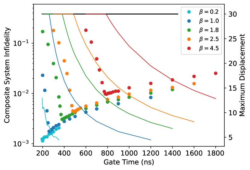
and the Broyden–Fletcher–Goldfarb–Shanno (BFGS) algorithm [28]. The qubit’s geometric phase is then corrected by applying a virtual rotation around the z-axis on the resulting state. In Fig. 1, the infidelity resulting from our standard ECD gate’s optimization is shown as a function of gate time for a selection of values of the target . For any chosen target , an optimal gate duration can be found at the smallest gate duration where the maximum displacement achieved during the gate is not saturated by . For gate durations shorter than the optimal gate duration, the increasing infidelities are due to the saturation of , which causes a mismatch between the achieved and the target . For gate durations longer than the optimal gate duration, the increasing infidelities are due to the increasing impact of the decoherence channels for longer ECD gate durations.
For every target , the optimal gate duration is found and the optimized pulse’s infidelity is computed (see Fig. 3; we remind the reader that this plot appears in a later section because it is compared with results of numerical optimizations yet to be described). This infidelity is computed by averaging the gate infidelity applied over 96 initial quantum states that form an overcomplete basis of displaced coherent states. For , the gate duration is fixed at ns, which is the minimum gate duration possible given the considered pulse primitives. The amplitude of the cavity’s displacement pulses is then reduced to achieve the target . Attempting to reduce the gate duration below our fixed minimum of ns would result in Gaussian pulses overlapping with each other and the qubit’s pulse, which can skew the overall pulse shape. This prevents the standard ECD gate from reaching the approximate gate time derived in Section II.1 in the regime of (see Fig. 3). For , the gate duration is set to the smallest possible value that complies with the constraint, which, as shown in Fig. 1, yields the best gate infidelity in our numerical simulations. In that regime, our optimized standard ECD pulses closely follow the approximate gate times (see Fig. 3).
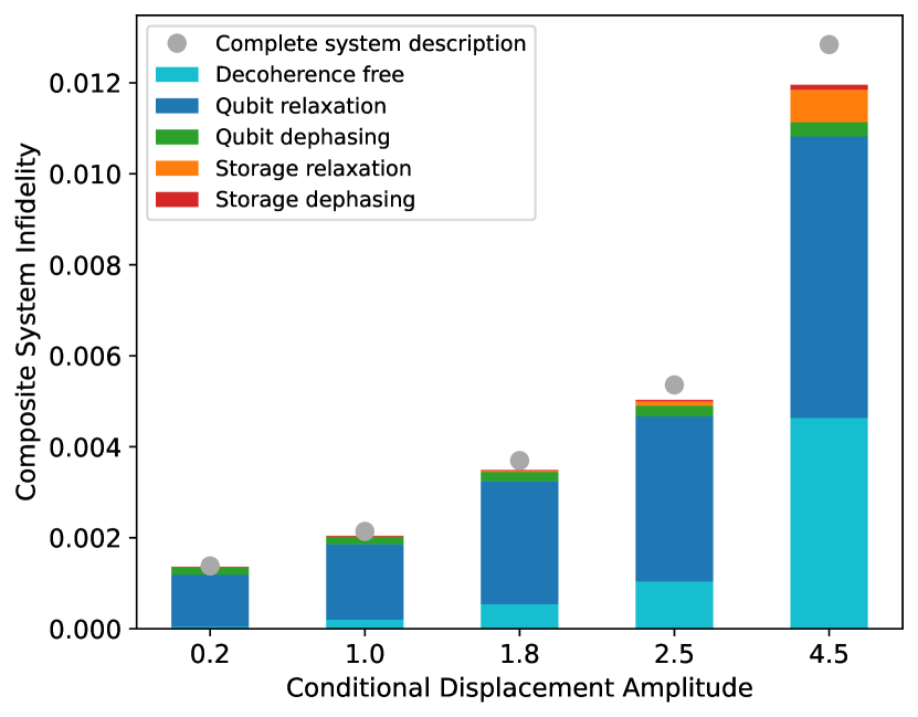
Figure 2 shows the error budget of our standard ECD gate’s construction, computed by including a single decoherence channel at a time in each of the simulations and removing the decoherence-free contribution from the infidelity. The infidelity is dominated by the qubit’s relaxation rate for all values of , but an increasing effect of the cavity’s decoherence channels and decoherence-free mechanisms is observed with increasing value of . A small mismatch is also observed between the sum of each decoherence channel’s contribution and the total infidelity of all the decoherence channels. This could be explained by the compounding effects of having certain combinations of decoherence channels.
II.4 Relaxing the No-Overlap Constraint
We now propose an alternative construction for an ECD gate, where primitives are allowed to overlap with one another. By relaxing the no-overlap constraint that was applied to our standard ECD gate’s construction, the pulse can be optimized to a shorter gate time in the regime, as shown in Fig. 3. We call these pulses “overlapping primitives pulses” (OP pulses).
For this optimization, the starting time for the second and third Gaussian primitives applied to the cavity, and , are added to the variational parameters for the optimization. The first and last primitives remain locked at the start and at the end of the ECD gate, respectively. The parameters are optimized against the objective function Eq. (15), which is used in the final optimization round of the construction of our standard ECD gate. Given a target , we iteratively optimize the parameters while reducing the total gate time by steps of ns, until no gain is observed in the gate fidelity. The resulting parameters in each round of optimization are used as initial conditions for optimizing the gate given the subsequent target gate time, with the exception of , for which the initial value is reduced by at every step. The pulse remains locked at the centre of the gate.
Figure 3 shows the gate time as a function of target conditional displacement amplitude and the corresponding pulses’ infidelities. The curve no longer plateaus in the small regime and instead follows the approximate gate times closely for all values of . The second and third Gaussian primitives now overlap with the pulse applied on the qubit, but no significant impact is observed in the infidelity for all values of the conditional displacement amplitude considered.
III Optimal Control for an ECD Gate
In this section, we present an optimal-control approach that reduces the problem of constructing ECD gates to an optimization problem. We then compare the resulting pulse shapes to the OP pulse shapes. In addition, we compare the resulting gate times to the approximate and standard gate times as described above.
III.1 The Optimization Problem
Due to the truncated dimensions of the cavity’s Hilbert space, not all quantum states will evolve properly under the given truncated Hamiltonian, for example, the state for . Therefore, we choose the average infidelity over a subset of operator basis states as our objective function. We choose this approach over more-standard objective functions, such as the average gate fidelity over a complete basis set [29], which are computationally too costly, as they require a large number of evaluation rounds of the objective function. An alternative objective function could be the infidelity between a target unitary operator and the resulting unitary operator. However, the computed unitary operator may again be unreliable due to the truncated dimensions of the cavity, and is not easily parallelizable.
To determine , we first construct a pulse shape for a standard ECD gate for the target . Then, the product states of the overcomplete coherent states for a bosonic system [30] and the operator basis states for a qubit [29] are chosen as the initial states. After evolving the initial states using the pulse shape of a standard ECD gate, we select the initial states that result in an infidelity that is lower than a selected threshold to be members of . Thus, the goal of the optimization problem is to find the optimal fields that drive the ensemble of initial states into the corresponding target states in a total gate time , with an objective function that penalizes deviations from the following constraints: the maximum displacement shift in the cavity to not be greater than a threshold and the pulse shape vanishing at the both the start and the end of the gate. We define our objective function as
| (16) |
where is the fixed total gate time, represents all the coefficients constructing the pulse shape in Eq. (20) in Subsection (III.2), and the objective functions are defined as follows.
-
•
The first objective function is the average infidelity over :
(17) -
•
The maximum displacement shift of the cavity must be smaller than the threshold , so we use a sigmoid function to penalize for the values of that exceed the threshold, which leads to the objective function
(18) where is a hyperparameter.
-
•
The displacement shift of the cavity at the end of the evolution is penalized so as to stay close to zero so that in consecutive applications of ECD gates (e.g., in preparing GKP states as described in Section IV) the value remains small at both the beginning and the end of each ECD gate:
(19)
Note that the control amplitude of and of are included in the cost function to force them to be as close to zero as possible following the transformations applied during the pulse shape construction. Also note that we optimize pulse shapes for .
III.2 Construction of Pulse Shapes
For the sake of computational efficiency, control pulses can be parameterized by a set of basis functions, for example, Fourier functions or B-spline functions. Following Ref. [31], we use quadratic B-spline basis functions with equidistant centres as the basis functions such that no more than three of them are nonzero at any point in time. This allows the control functions to be evaluated efficiently. The parameterized pulse shapes can be written as , with
| (20) |
where and are real coefficients, are the B-spline functions, and is the number of B-spline functions and will be determined later. Furthermore, the maximum amplitude of the pulses is bounded by applying the transformation to the original pulses.
The pulses applied on the cavity are also are chosen to be symmetric around the midpoint . Therefore, the pulse shape at the time segment is mirrored and a butterfly low-pass filter of order 6 with a bandwidth set to MHz is applied to the generated pulse. This achieves two outcomes: the resulting pulse shape is smooth at the midpoint and the bandwidth of the pulses abides by experimental limitations.
For each target , we set the initial gate time to be equal to the time of an optimized standard ECD gate. To determine the number of basis functions , we fit the above-mentioned ansatz to the standard ECD gate pulse shape and choose the smallest possible value for that matches the infidelity of the standard ECD gate. We do this to reduce the experimental overhead and decrease the total computation time of the optimization process.
Because the ECD gate is only defined up to a virtual gate, the control pulse of the qubit is fixed to be a single pulse as is done in the standard construction. Optimizing the entire pulse results in pulse shapes without any relevant contribution to the resulting unitary evolution (not shown in this paper).
Because we have a larger number of variables for the optimization problem compared to the standard construction, we use the limited-memory variant of BFGS with boundaries (L-BFGS-B) [32] implemented in SciPy [33], and we pass auto-differentiated gradients of the objective function to the optimizer using Jax [34]. For each round of optimization given a target , the pulse shape is randomly initialized. We then use the resulting parameters in the subsequent optimization round, but for a shorter pulse shape with a new total time , using ns. For a sufficiently small value of , the optimization for a shorter gate time nearly always converges faster than an optimization with a random initialization of the parameters.
III.3 Numerical Results
The gate time and infidelity as a function of the parameter resulting from our pulse-shaping method are shown in Fig. 3. In the regime , our optimal-control pulses, the standard pulses, and the OP pulses converge to having almost identical gate times. The small discrepancy between the OP pulses and the optimal-control pulses is explained by the fact that the optimal-control parameters are initialized randomly for the first choice of given each , while the OP pulses are initialized from a physically well-informed guess. However, in the regime , the optimal-control pulses outperform the other pulse shapes by a small amount and outperform the approximate gate time derived in Section II.1. In particular, in the regime , the optimal-control pulses continue to improve the gate time as is decreased without compromising the infidelity of any of the resulting gates.
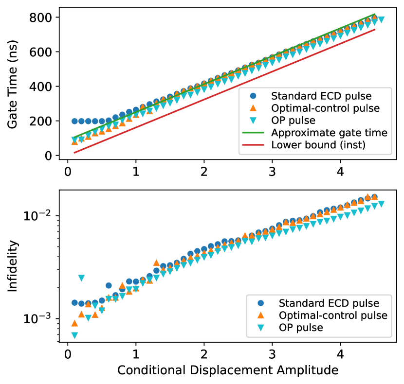
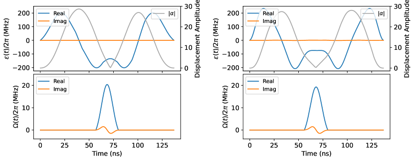
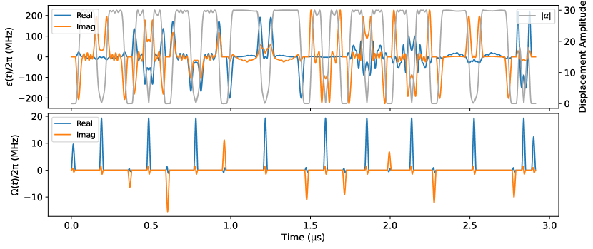
Figure 4 (right side) shows the pulse shape optimized for the ECD gate with a target . We observe that, similar to the case of OP pulse shapes (Fig. 4, left side), the two Gaussian pulses in the vicinity of the middle point and the pulse on the qubit overlap in time. This combination reduces the total gate time. Note that the qubit’s pulse is applied while the cavity is displaced from the vacuum state. However, in the standard construction, we avoid applying a pulse when the cavity is displaced, as it may be miscalibrated due to the displacement of the cavity and the dispersive coupling. However, given the fact that the final average state’s fidelity of both the ECD gate with overlapping primitives and the pulse-shaping ECD gate are better than that of the standard ECD gate, we conclude that this effect does not obstruct the performance of our pulses. The overlap between different primitive-like pulses in the optimal-control pulses explains the small offset between our gate times and the approximate gate times derived in Sec. II.1.
In addition, the phase space trajectories generated by our optimal-control pulses are similar to those of both the standard and OP pulses, as shown by the resulting displacement amplitude throughout the evolution (see the grey curve in Fig. 4). The pulse shapes consist of a fast displacement far from the origin, a free evolution if needed, and another displacement to return the state to the origin in the phase space before applying the pulse on the qubit and repeating another sequence of two displacements. These trajectories, along with the results shown in Fig. 3, suggest that the ECD gate with overlapping primitives is a “bang–bang” control scheme [35].
IV Circuit Optimization for the Preparation of a GKP State
In this section, we showcase how the optimized pulse shapes for ECD gates with small values of can be utilized to reduce the total preparation time of a logical state. This state has been reported to be prepared in approximately s with a quantum circuit composed of nine ECD gates and 10 single-qubit rotations [21]. In Fig. 3, it is shown that the gate time is nearly proportional to the magnitude of the parameter of the ECD gate. To minimize the GKP state preparation time, we take advantage of these shorter ECD gates by incentivizing the choice of smaller values of for a sequence of ECD gates using the objective function
| (21) |
where is a hyperparameter. The reduced density matrix for the cavity at the end of the state preparation is , and the target cavity state is .
After obtaining the optimized circuit parameters for the preparation protocol, the optimized ECD gates’ pulses for the resulting values of are concatenated to realize fast preparation of a GKP state. We construct each ECD gate by multiplying the optimized pulse shape for each real value of by a phase coefficient. A virtual rotation gate is applied after each ECD gate, prior to each subsequent qubit rotation, to compensate for the geometric phase, which is not taken into account in our pre-optimized ECD gates from the previous section. The entire sequence for preparing a state is shown in Fig. 5 and the corresponding , , } parameters are shown in Table 1. The total preparation time is s and the closed-system cavity fidelity is 0.978.
By applying the optimized pulse shapes for ECD gates, the preparation sequence can be reduced by over 300 ns. Given that the gate time of ECD gates for large values of is close to that of standard ECD gates, only the ECD gates with small value of are replaced by optimal-control pulses, in order to reduce experimental characterization efforts.
V Conclusion
We have provided a detailed analysis of a standard ECD gate and compared it with an alternative construction where primitives are allowed to overlap and with optimal-control pulses that result from our numerical optimizations. Both the OP pulses and the optimal-control pulses provide a small improvement in the gate time of an ECD gate for small values of , and our results suggest that the current standard pulse is near optimal otherwise. Using our optimized pulses for small values of , a greater number of stabilization rounds can be performed on GKP states, as the state-of-the-art protocols, such as the sBs protocol [11], include ECD gates with small values of which are executed many times during an experiment.
ACKNOWLEDGEMENTS
We thank our editor, Marko Bucyk, for his careful review and editing of the manuscript. We thank Marc-Antoine Lemonde, Dany Lachance-Quirion, and Julien Camirand Lemyre at Nord Quantique for helpful discussions on numerical simulations of a bosonic system and the construction of a standard ECD pulse shape. M. L.-M. further acknowledges the financial support of Mitacs. P. R. acknowledges the financial support of Mike and Ophelia Lazaridis, Innovation, Science and Economic Development Canada (ISED), and the Perimeter Institute for Theoretical Physics. Research at the Perimeter Institute is supported in part by the Government of Canada through ISED and by the Province of Ontario through the Ministry of Colleges and Universities.
References
- Braunstein and van Loock [2005] S. L. Braunstein and P. van Loock, Quantum information with continuous variables, Reviews of Modern Physics 77, 513 (2005).
- Bergmann and van Loock [2016] M. Bergmann and P. van Loock, Quantum error correction against photon loss using multicomponent cat states, Physical Review A 94, 042332 (2016).
- Li et al. [2017] L. Li, C.-L. Zou, V. V. Albert, et al., Cat Codes with Optimal Decoherence Suppression for a Lossy Bosonic Channel, Physical Review Letters 119, 030502 (2017).
- Michael et al. [2016] M. H. Michael, M. Silveri, R. T. Brierley, et al., New Class of Quantum Error-Correcting Codes for a Bosonic Mode, Physical Review X 6, 031006 (2016).
- Grimsmo et al. [2020] A. L. Grimsmo, J. Combes, and B. Q. Baragiola, Quantum Computing with Rotation-Symmetric Bosonic Codes, Physical Review X 10, 011058 (2020).
- Gottesman et al. [2001] D. Gottesman, A. Kitaev, and J. Preskill, Encoding a qubit in an oscillator, Physical Review A 64, 012310 (2001).
- Flühmann et al. [2019] C. Flühmann, T. L. Nguyen, M. Marinelli, et al., Encoding a qubit in a trapped-ion mechanical oscillator, Nature 566, 513 (2019).
- Campagne-Ibarcq et al. [2020] P. Campagne-Ibarcq, A. Eickbusch, S. Touzard, et al., Quantum error correction of a qubit encoded in grid states of an oscillator, Nature 584, 368 (2020).
- Royer et al. [2022] B. Royer, S. Singh, and S. M. Girvin, Encoding qubits in multimode grid states, PRX Quantum 3, 010335 (2022).
- De Neeve et al. [2022] B. De Neeve, T.-L. Nguyen, T. Behrle, and J. P. Home, Error correction of a logical grid state qubit by dissipative pumping, Nature Physics 18, 296 (2022).
- Royer et al. [2020] B. Royer, S. Singh, and S. M. Girvin, Stabilization of Finite-Energy Gottesman–Kitaev–Preskill States, Physical Review Letters 125, 260509 (2020).
- Sivak et al. [2023] V. Sivak, A. Eickbusch, B. Royer, et al., Real-time quantum error correction beyond break-even, Nature 616, 50 (2023).
- Lachance-Quirion et al. [2024] D. Lachance-Quirion, M.-A. Lemonde, J. O. Simoneau, et al., Autonomous quantum error correction of Gottesman–Kitaev–Preskill states, Physical Review Letters 132, 150607 (2024).
- Fowler et al. [2012] A. G. Fowler, M. Mariantoni, J. M. Martinis, and A. N. Cleland, Surface codes: Towards practical large-scale quantum computation, Physical Review A 86, 032324 (2012).
- Andersen et al. [2020] C. K. Andersen, A. Remm, S. Lazar, et al., Repeated quantum error detection in a surface code, Nature Physics 16, 875 (2020).
- Google Quantum AI [2023] Google Quantum AI, Suppressing quantum errors by scaling a surface code logical qubit, Nature 614, 676 (2023).
- Noh and Chamberland [2020] K. Noh and C. Chamberland, Fault-tolerant bosonic quantum error correction with the surface–Gottesman–Kitaev–Preskill code, Physical Review A 101, 012316 (2020).
- Law and Eberly [1996] C. K. Law and J. H. Eberly, Arbitrary Control of a Quantum Electromagnetic Field, Physical Review Letters 76, 1055 (1996).
- Grimm et al. [2020] A. Grimm, N. E. Frattini, S. Puri, et al., Stabilization and operation of a Kerr-cat qubit, Nature 584, 205 (2020).
- Gao et al. [2019] Y. Y. Gao, B. J. Lester, K. S. Chou, et al., Entanglement of bosonic modes through an engineered exchange interaction, Nature 566, 509 (2019).
- Eickbusch et al. [2022] A. Eickbusch, V. Sivak, A. Z. Ding, et al., Fast universal control of an oscillator with weak dispersive coupling to a qubit, Nature Physics 18, 1464 (2022).
- Hastrup et al. [2021] J. Hastrup, K. Park, J. B. Brask, et al., Measurement-free preparation of grid states, npj Quantum Information 7, 17 (2021).
- Berry [1984] M. V. Berry, Quantal Phase Factors Accompanying Adiabatic Changes, Proceedings of the Royal Society of London. A. Mathematical and Physical Sciences 392, 45 (1984).
- Lescanne et al. [2019] R. Lescanne, L. Verney, Q. Ficheux, et al., Escape of a driven quantum Josephson circuit into unconfined states, Physical Review Applied 11, 014030 (2019).
- Sank et al. [2016] D. Sank, Z. Chen, M. Khezri, et al., Measurement-Induced State Transitions in a Superconducting Qubit: Beyond the Rotating Wave Approximation, Physical Review Letters 117, 190503 (2016).
- Reed et al. [2010] M. Reed, L. DiCarlo, B. Johnson, et al., High-Fidelity Readout in Circuit Quantum Electrodynamics Using the Jaynes-Cummings Nonlinearity, Physical Review Letters 105, 173601 (2010).
- Motzoi et al. [2009] F. Motzoi, J. Gambetta, P. Rebentrost, and F. Wilhelm, Simple Pulses for Elimination of Leakage in Weakly Nonlinear Qubits, Physical Review Letters 103, 110501 (2009).
- Fletcher [2013] R. Fletcher, Practical Methods of Optimization (John Wiley & Sons, 2013).
- Nielsen [2002] M. A. Nielsen, A Simple Formula for the Average Gate Fidelity of a Quantum Dynamical Operation, Physics Letters A 303, 249 (2002).
- Klauder [1960] J. R. Klauder, The action option and a Feynman quantization of spinor fields in terms of ordinary c-numbers, Annals of Physics 11, 123 (1960).
- Petersson et al. [2020] N. A. Petersson, F. M. Garcia, A. E. Copeland, et al., Discrete Adjoints for Accurate Numerical Optimization with Application to Quantum Control, arXiv:2001.01013 (2020).
- Liu and Nocedal [1989] D. C. Liu and J. Nocedal, On the limited memory BFGS method for large scale optimization, Mathematical Programming 45, 503 (1989).
- Virtanen et al. [2020] P. Virtanen, R. Gommers, T. E. Oliphant, M. Haberland, T. Reddy, D. Cournapeau, E. Burovski, P. Peterson, W. Weckesser, J. Bright, et al., SciPy 1.0: fundamental algorithms for scientific computing in python, Nature methods 17, 261 (2020).
- Bradbury et al. [2018] J. Bradbury, R. Frostig, P. Hawkins, et al., JAX: composable transformations of Python+NumPy programs, Version 0.3.13 (2018).
- Rolewicz [2013] S. Rolewicz, Functional Analysis and Control Theory: Linear Systems, Vol. 29 (Springer Science & Business Media, 2013).