Probing the nature of dark matter using strongly lensed gravitational waves from binary black holes

Abstract

Next-generation ground-based gravitational-wave (GW) detectors are expected to detect millions of binary black hole mergers during their operation period. A small fraction ($\sim 0.1-1\%$) of them will be strongly lensed by intervening galaxies and clusters, producing multiple copies of the GW signals. The expected number of lensed events and the distribution of the time delay between lensed images will depend on the mass distribution of the lenses at different redshifts. Warm dark matter or fuzzy dark matter models predict lower abundances of small mass dark matter halos as compared to the standard cold dark matter. This will result in a reduction in the number of strongly lensed GW events, especially at small time delays. Using the number of lensed events and the lensing time delay distribution, we can put a lower bound on the mass of the warm/fuzzy dark matter particle from a catalog of lensed GW events. The expected bounds from GW strong lensing from next-generation detectors are significantly better than the current constraints.

Introduction:—

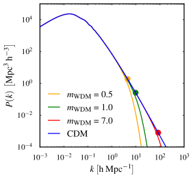
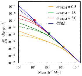
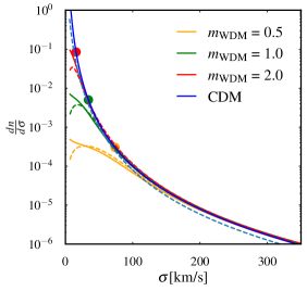
Figure 1: Left panel: The power spectrum of linear perturbations as predicted by the CDM model as well as the WDM model with different values of $m_{\textsc{wdm}}$ (in keV). Half-mode scales for different $m_{\textsc{wdm}}$ are shown by the filled circles. Middle panel: HMF for CDM and WDM at redshift $z=0$. Solid and dashed lines represent the Behroozi Behroozi et al. (2013) and Jenkins Jenkins et al. (2001) HMF models, respectively. Note the suppression in the number density of lower mass halos in the WDM model. Filled circles with different colours denote the half mode mass scale for different $m_{\textsc{wdm}}$. Right panel: The distribution of the velocity dispersion of lenses produced by the CDM and WDM halos. Here also the solid and dashed lines represents the Behroozi and Jenkins HMF models. Reduction in number density is reflected as reduction of the low $\sigma$ halos. Filled circles denote the velocity dispersion of the corresponding half mode mass.

A variety of astronomical observations have firmly established that $\sim 25\%$ of the mass energy in the universe is in the form of some non-baryonic dark matter (DM) Bertone and Hooper (2018). Particle physicists and cosmologists have come up with several candidates for DM, spanning a very wide mass range. The list of candidates ranges from extremely light elementary particles Bertone and Hooper (2018); Arbey and Mahmoudi (2021) to supermassive primordial black holes Carr and Kühnel (2022).

DM candidates can be classified according to their velocity dispersion, which defines a free streaming length scale. Below this length scale all the cosmological density perturbations are wiped out, so no structure can form in the universe below this length scale. Cold DM (CDM), such as the weakly interacting massive particles Griest and Kamionkowski (2000), axions Feng (2010) and primordial black holes Green and Kavanagh (2021), has small free streaming length scales and does not affect the cosmological structure formation. On the other hand, hot DM such as neutrinos is highly relativistic. Free streaming of such relativistic particles would erase perturbations in the matter density even on the scale of galaxy clusters ($\sim 10^{15}\mathrm{M}_{\odot}$). The very existence of such large scale structures has ruled out hot DM White et al. (1983). In between there exists another class, called warm DM (WDM), such as gravitino Kawasaki et al. (1997) and sterile neutrino Boyarsky et al. (2019). They are non-relativistic but still have non-negligible velocity dispersion. They have shorter free streaming length than regular neutrinos, and can erase structure on galaxy scales. Thus the existence of galaxies can put some (rather weak) constraints on the mass of the WDM particle.

In the past decades, the cosmological constant dominated CDM model known as $\Lambda$CDM, has emerged as the standard model of cosmology Komatsu et al. (2011); Cole et al. (2005); Tegmark et al. (2006). However, despite decades of effort, neither direct laboratory experiments or indirect astronomical observations have been able to detect any CDM candidates so far. In addition, though $\Lambda$CDM predictions match with observed large scale structure, sub-galactic observations might be in conflict with the predictions of this model. One is the apparent under-abundance of satellites in the Milky Way, as compared to the earlier CDM simulations, called the “missing satellite problem” Kauffmann et al. (1993); Klypin et al. (1999); Moore et al. (1999); Bode et al. (2001) . The second, known as the “core-cusp problem,” is the observed discrepancy between the inferred DM density profiles of low-mass galaxies and that predicted by CDM simulations de Blok (2010). Simulations typically predict “cuspy” profiles (steep density profiles at the center) while observations suggest the existence of “cores” (softer density profiles at the center).

While some of these apparent discrepancies between CDM models and observations could be attributed to astrophysical reasons (such as the effect of baryons), several new DM candidates have also been proposed to address them. WDM is the simplest departure from CDM, endowing the DM with a small velocity dispersion. WDM particle with a mass in $\mathrm{keV}$ range predicts the suppression of structures at small scales ($\sim 100\;\mathrm{kpc}$) without affecting the large scales ($\sim\mathrm{Mpc}$), thus explaining the missing satellites. Another model, called ”self-interacting DM” Spergel and Steinhardt (2000), adds a self-interaction cross-section to the DM. The resulting elastic scattering between the DM particles in the inner galactic regions redistributes energy, producing the effect of a core. Fuzzy DM (FDM) particles are ultralight bosons (mass $\sim 10^{-22}\;\mathrm{eV}$), with de Broglie wavelength larger than the inter-particle separation. The resulting wave-like behaviour leads to formation of solitonic cores at the center of haloes and density granules on scales smaller than $\sim\mathrm{kpc}$ are erased, while large scale structure is indistinguishable from CDM Hu et al. (2000).

The observation of Lyman-$\alpha$ forest — absorption lines in the distant quasar spectra induced by neutral hydrogen along the line of sight — provides the strongest lower limit ($m_{\textsc{wdm}}>3-5\;\mathrm{keV}$) on the WDM mass Viel et al. (2013); Markovič and Viel (2014); Yèche et al. (2017); Villasenor et al. (2023). Combining this with strong gravitational lensing Vegetti et al. (2023) and the abundance of Milky Way satellites has resulted in a joint constraint $m_{\textsc{wdm}}>6.048\;\mathrm{keV}$ Enzi et al. (2021). Different cosmological datasets puts upper bound $m_{\psi}\geq 10^{-22}\;\mathrm{eV}$ on the mass of FDM Bozek et al. (2015); Schive et al. (2016); Corasaniti et al. (2017); Iršič et al. (2017). A stronger constraint, $m_{\psi}\geq(0.6-1)\times 10^{-19}\;\mathrm{eV}$ is obtained from the survival of an old star cluster in an ultra faint dwarf galaxy Eridaus II Marsh and Niemeyer (2019).

Gravitational-wave (GW) observations offer new probes of DM (see, e.g., Bertone et al. (2019)). The presence of a DM overdensity surrounding a black hole can have impact on the GWs emitted during the inspiral and merger with another compact object. The upcoming LISA observatory Amaro-Seoane and et al. (2017) will be able to detect the effect of the DM on the GW signal, offering a powerful probe of the nature of particle DM Kavanagh et al. (2020); Kadota et al. (2023); Bertone et al. (2019). Ultralight bosons, such as axions, can affect the mass and spin of black holes by forming gravitationally bound states around them Richard et al. (2015). GW emission from such objects could be detected by various GW detectors Arvanitaki and Dubovsky (2011); Arvanitaki et al. (2015); Brito et al. (2017); Baryakhtar et al. (2017). FDM can also be indirectly detected using pulsar timing arrays if the oscillation frequency falls within their detection band Porayko et al. (2018).

Gravitational lensing of GWs offer yet another avenue to probe the nature of DM (see, e.g. Dai et al. (2018); Oguri and Takahashi (2020); Choi et al. (2021); Gao et al. (2022); Guo and Lu (2022); Çalışkan et al. (2023); Cao et al. (2020); Cao, Shuo et al. (2022), for some recent work). The next-generation (XG) ground-based GW detectors will detect millions of binary black-hole mergers (BBH) out to high redshifts ($z\sim 10-100$) Hall and Evans (2019). About $0.1-1\%$ of them will be strongly lensed by the galaxies and clusters hosted in these DM halos, producing multiple copies of the GW signals. The time delay between the lensed copies of these GW signals can be accurately measured. The exact fraction of lensed mergers and the distribution of lensing time delay will depend on the mass distribution of lenses at various redshifts Xu et al. (2022) as well as cosmological parameters Jana et al. (2023). In this letter, we propose a statistical probe to constrain the mass of the WDM particle using a catalogue of strongly lensed GW detections. If the DM is warm, this will hinder the formation of low-mass halos. This suppression in the the abundance of low-mass halos will result in a reduction in the number of lensed events with small time delays, as small time delays are mostly produced by low mass lenses.

Our proposal is to look for the imprints of WDM on the number of lensed signals, as well as on the distribution of their time delays. This approach is closely connected to our earlier work Jana et al. (2023) on constraining the cosmological parameters from strongly lensed GW signals. Our method does not rely on the accurate knowledge of the source location of the individual signals or the properties of the corresponding lenses. Indeed, the number of lensed events as well as the time delay distribution will also depend on the distribution of source properties (e.g., mass and redshift distribution of BBHs Haris et al. (2018); Li et al. (2018); Mukherjee et al. (2021)) as well as the lens properties (e.g., the mass function of the DM halos Robertson et al. (2020) and the lens model Janquart et al. (2022); More and More (2022)). If the distributions of the source and lens properties are known from other observations or theoretical models (e.g., from the observation of unlensed GW signals and cosmological simulations), then the mass of the WDM can be inferred from the observed number of lensed events and their time delay distribution.

We forecast that BBH observations during $10\;\mathrm{yrs}$ of operation of XG detectors Maggiore et al. (2020); Reitze et al. (2019) will be to provide constraints ($m_{\textsc{wdm}}^{-1}<0.035-0.056~{}\mathrm{keV}^{-1}$) are significantly better than the current constraints ($m_{\textsc{wdm}}>3-5\;\mathrm{keV}$). We simply translate the constraints on $m_{\textsc{wdm}}$ to mass of FDM particle ($m_{\psi}$). An optimistic assumption of merger rate will give us the constraint $m_{\psi}>7.3\times 10^{-19}{\mathrm{eV}}$, which is almost three order of magnitude improvement over existing bounds.

Warm dark matter:—

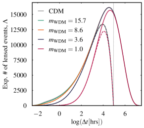
Figure 2: Expected distributions of time delay between strongly lensed GW signals, corresponding to different values of $m_{\textsc{wdm}}$. Note the suppression in number of lensed events compared to CDM, especially for lower time delays, which is the reflection of absence of the lower mass halos for smaller $m_{\textsc{wdm}}$. The time delay distributions measurable from an observation period of $10\;\mathrm{yrs}$ are shown by dashed lines. The vertical line indicates the period of $10\;\mathrm{yrs}$.

Free streaming of WDM particles suppress primordial perturbations at scales smaller than the free streaming scale. Fitting functions for modelling the WDM transfer function have been proposed in different studies Bardeen et al. (1986); Bode et al. (2001); Viel et al. (2005). They give us a prescription to convert the power spectrum $P_{\textsc{cdm}}(k)$ of linear perturbations in the CDM model to the same in the WDM model [$P_{\textsc{wdm}}(k)$], through the transfer function. We use the transfer function given in Viel et al. (2005),

$$T(k)=\left[\frac{P_{\textsc{cdm}}(k)}{P_{\textsc{wdm}}(k)}\right]^{1/2}=\left[1+(\alpha k)^{2\mu}\right]^{-5/\mu},$$ (1)

where $\mu=1.12$ and

$$\alpha=0.049\left(\frac{m_{\textsc{wdm}}}{\mathrm{keV}}\right)^{-1.11}\left(\frac{\Omega_{\textsc{wdm}}}{0.25}\right)^{0.11}\left(\frac{h}{0.7}\right)^{1.22}~{}h^{-1}\mathrm{Mpc}$$ (2)

is called the effective free streaming scale. Above, $\Omega_{\textsc{wdm}}$ is the energy density in the form of WDM and $h$ is the Hubble constant in units of 100 km/s/Mpc. We can introduce another length scale, called half mode length scale $\lambda_{\mathrm{hm}}$, where the WDM transfer function becomes half: $\lambda_{\mathrm{hm}}=2\pi\alpha\,(2^{{\mu}/{5}}-1)^{-{1}/{2\mu}}$. This length scale introduces a half mode mass scale $M_{\mathrm{hm}}=\frac{4\pi}{3}\bar{\rho}\,({\lambda_{\mathrm{hm}}}/{2})^{3}$, where $\bar{\rho}$ is the averaged density of the halo. Abundances of DM haloes with mass below the $M_{\mathrm{hm}}$ will be suppressed compared to CDM, while the masses above $M_{\mathrm{hm}}$ are unaffected.

We use different halo mass functions (HMFs) that model the comoving number density $dn_{\textsc{cdm}}/dM$ of CDM halos in different mass ranges. Given a HMF in CDM, the same in WDM model for a particular $m_{\textsc{wdm}}$ is obtained using the fitting formula given in Schneider et al. (2012)

$$\frac{dn_{\textsc{wdm}}/dM}{dn_{\textsc{cdm}}/dM}=\left(1+\frac{M_{\mathrm{hm}}}{M}\right)^{-\beta},$$ (3)

where $\beta=1.16$. The dependence on $m_{\textsc{wdm}}$ comes through $M_{\mathrm{hm}}$. To obtain HMF in WDM model, we use HMFcalc package Murray et al. (2013). For our main analysis we consider the Behroozi Behroozi et al. (2013) model of the CDM HMF. In order to estimate the effect of using an incorrect CDM HMF model, we also consider the Jenkins Jenkins et al. (2001) model of the same implemented in the same package.

These DM halos acts as gravitational lenses that deflect light as well as GWs. In this letter, we are concerned about the strong lensing of GWs that produces multiple copies of the GW signals. We approximate these halo lenses as singular isothermal spheres (SISs) Peter Schneider (1999), parameterised by their dispersion velocity $\sigma$. We assume that the halos are spherically symmetric and virialised, with average density $\bar{\rho}$ and radius $R$. This allows us to compute the dispersion velocity of the SIS lens from the halo mass

$$\sigma\simeq\sqrt{\frac{GM}{R}},~{}~{}~{}M=\frac{4}{3}\pi R^{3}\bar{\rho}.$$ (4)

Figure 1 shows the the power spectrum, the HMF and the $\sigma$ distribution of lenses derived from the HMF, as predicted by the CDM model as well as the WDM model corresponding to different WDM masses. These can be use to compute the expected number of strongly lensed GW signals and the distribution of the time delay between the lensed copies of GW signals.

Figure 2 shows the expected number of lensed events $\Lambda(m_{\textsc{wdm}})$ and the time delay distribution $p(\Delta t|m_{\textsc{wdm}})$ as a function of $m_{\textsc{wdm}}$. We can see that $\Lambda$ decreases with decreasing $m_{\textsc{wdm}}$. This is due to the fact that there will be a smaller number of low-mass halos for lower $m_{\textsc{wdm}}$. The absence of lower mass halos is reflected in the time delay distribution as the reduction in the of lower time delays. Using these differences in the time delay distribution and total number of lensed events, we will be able to either measure the mass of the WDM particle, or put a lower bound on $m_{\textsc{wdm}}$. In practice, we put an upper bound on $m_{\textsc{wdm}}^{-1}$ since it has a convenient lower bound of zero.

Expected constraints on warm DM:—

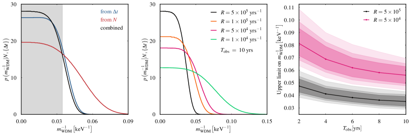
Figure 3: Left panel: Posterior distribution of $m_{\textsc{wdm}}^{-1}$ computed from number of lensed events and time delay distribution separately, along with the combined posterior, using simulated observations generated assumming $\Lambda$CDM universe. Here we assumed a BBH detection rate of $R=5\times 10^{5}\;\mathrm{yr}^{-1}$ and $T_{\mathrm{obs}}=10\mathrm{yrs}$. Gray shaded region represents the $90\%$ quantile of the combined posterior, yielding an upper limit of $m_{\textsc{wdm}}^{-1}\leq 0.035$. Middle panel: Combined constraints from GW lensing on $m_{\textsc{wdm}}^{-1}$ assuming different detection rates with observation time period $T_{\mathrm{obs}}=10\;\mathrm{yrs}$. Right panel: 38%, 50% and 68% credible intervals (denoted by different shades) of the distributions of 90% upper limit of $m_{\textsc{wdm}}^{-1}$ obtained from $\sim 1000$ recovery tests for different values of $R$ and $T_{\mathrm{obs}}$.

We first ask the question: if the DM is actually cold (i.e., $m_{\textsc{wdm}}^{-1}=0$), how well can we constrain $m_{\textsc{wdm}}^{-1}$ using future obervations of lensed GWs. In order to answer this, we simulate a population of BBH mergers with redshift distribution given by Dominik et al. (2013). We assume a BBH detection rate $R=5\times 10^{5}\;\mathrm{yr}^{-1}$ and an observation period $T_{\mathrm{obs}}=10\;\mathrm{yrs}$. We neglect the selection effects in detection, as XG detectors are anticipated to detect all the BBH mergers out to large red shifts ($z\sim 10-100$). The mass distribution of the lenses at various redshifts are described by the CDM HMF model of Behroozi et al. (2013). Lenses as modelled using the SIS model, using Eq. (4) for converting the halo mass to the velocity dispersion of the lens. This allows us to compute the the strong lensing optical depth for sources located at different redshifts, which can be convolved with the redshift distribution of the BBH mergers to to compute the expected number $\Lambda$ of lensed events. We assume the following values of cosmological parameters: $\Omega_{m}=0.316,H_{0}=67.3,\sigma_{8}=0.816~{}$Aghanim et al. (2020).

To simulate one observing scenario with $N$ detections of lensed events, we draw one sample from a Poisson distribution with mean $\Lambda$. Further, we draw samples $\{\Delta t_{i}\}_{i=1}^{N}$ from $p(\Delta t~{}|~{}m_{\textsc{wdm}}^{-1}\simeq 0,T_{\mathrm{obs}})$. Using $N$ and $\{\Delta t_{i}\}_{i=1}^{N}$ we evaluate the likelihoods $p\left(N~{}|~{}m_{\textsc{wdm}}^{-1},T_{\mathrm{obs}}\right)$ and $p\left(\{\Delta t_{i}\}~{}|~{}m_{\textsc{wdm}}^{-1},T_{\mathrm{obs}}\right)$. We assume uniform priors on $m_{\textsc{wdm}}^{-1}$, so final posterior is given by the product of two likelihoods. Figure 3 (left panel) shows the two likelihoods and the posteriror obtained from combining these two likelihoods. The $90\%$ quantile of combined posterior is shown in the shaded region, yielding an upper limit $m_{\textsc{wdm}}^{-1}<0.035~{}\mathrm{keV}^{-1}$.

The GW detection rate of XG detectors is uncertain as of now. For more conservative forecasts, we repeated the analysis with lower rates. Figure 3 (middle panel) shows the combined posteriors for different detection rates. As expected, with reduced rates the posteriors are broader. The 90% upper limits on $m_{\textsc{wdm}}^{-1}$ in are $0.047,0.055,0.082~{}\mathrm{keV}^{-1}$ for merger rates $10^{5},5\times 10^{4},10^{4}$, respectively. Constraints corresponding to different merger rates and observation periods are shown in Table 1. Since the upper limits depend on the realization of mock samples that are subjected to Poisson fluctuations, we repeat the observing scenario $\sim 1000$ times and compute the distribution of the 90% limit of $m_{\textsc{wdm}}^{-1}$. Figure 3 (right panel) shows the 38%, 50% and 68% quantiles of the distributions of the 90% upper limit of $m_{\textsc{wdm}}^{-1}$ for different observation time periods and merger rates.

	$2\;\mathrm{yrs}$	$4\;\mathrm{yrs}$	$6\;\mathrm{yrs}$	$8\;\mathrm{yrs}$	$10\;\mathrm{yrs}$
$5\times 10^{5}\;\mathrm{yr}^{-1}$	0.047	0.041	0.038	0.036	0.035
$1\times 10^{5}\;\mathrm{yr}^{-1}$	0.068	0.059	0.053	0.049	0.047
$5\times 10^{4}\;\mathrm{yr}^{-1}$	0.081	0.069	0.062	0.058	0.055

Table 1: Expected 90% credible upper limits on $m_{\textsc{wdm}}^{-1}$ in $\mathrm{keV}^{-1}$ for different merger rates $R$ and observation time periods $T_{\mathrm{obs}}$.

The FDM also predicts a cut-off in the HMF at small scales, through a mechanism that is dependent on the de Broglie wavelength rather than a free-streaming length. We translate the constraints on the $m_{\textsc{wdm}}$ to the mass of the FDM particle $m_{\psi}$ (Fig. 4). For this, we simply equate the half mode length scale of both. We use the expression of half mode length scale of FDM as given in Schive et al. (2016) which considers a transfer function given in Hu et al. (2000). We calculate half mode length scale for WDM using the HMFcalc package Murray et al. (2013) which uses the formula given in Schneider et al. (2012) and a transfer function given in Viel et al. (2005). This is just a simple translation, in order to be more rigorous, one needs to use the HMF in FDM. Even though approximate, this gives us an idea of the prospective constraints on FDM using future observations of GW strong lensing.

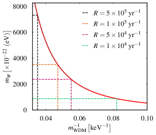
Figure 4: The relation between $m_{\psi}$ and $m_{\mathrm{wdm}}^{-1}$ obtained by equating the half mode length scale of FDM and WDM. Dashed vertical line shows the constraints on $m_{\mathrm{wdm}}^{-1}$ and corresponding dashed horizontal lines show the translated constraints on $m_{\psi}$. Different dashed lines are for different detection rates $R$, assuming $T_{\mathrm{obs}}=10\;\mathrm{yrs}$.

We also check whether we will be able to measure the mass of the DM particle when it is actually warm. To check this, we simulate an observing scenario using the HMF of the WDM model with mass $m_{\textsc{wdm}}=9~{}\mathrm{keV}$. Other details of the analysis are kept the same. We consider an optimistic ($R=5\times 10^{5}~{}\mathrm{yr}^{-1}$) and pessimistic ($R=5\times 10^{4}~{}\mathrm{yr}^{-1}$) detection rates. As seen in Fig. 5, the true value of $m_{\textsc{wdm}}$ is recovered within 68% credible interval.

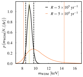
Figure 5: Posterior distribution of $m_{\textsc{wdm}}$ assuming that the true nature of the DM is described by the WDM model with $m_{\textsc{wdm}}=9~{}\mathrm{keV}$ (the yellow solid line in the middle). The plot shows the expected posteriors for $T_{\mathrm{obs}}=10\mathrm{yrs}$ assuming optimistic ($R=5\times 10^{5}~{}\mathrm{yr}^{-1}$) and pessimistic ($R=5\times 10^{4}~{}\mathrm{yr}^{-1}$) detection rates. Vertical dashed lines represent the 90% credible region of the posteriors.

Systematic errors:—

We have investigated various sources of systematic errors in deriving constraints on the nature of DM using future observations of strongly lensed GW signals.

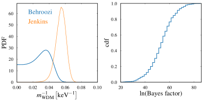
Figure 6: Left panel: Posterior distributions of $m_{\textsc{wdm}}^{-1}$ computed from number of lensed events and time delay distribution. The lensed events are simulated assuming a CDM HMF ($m_{\textsc{wdm}}^{-1}\simeq 0$) described by Behroozi model with merger rate $R=5\times 10^{5}\;\mathrm{yr}^{-1}$ and $T_{\mathrm{obs}}=10~{}\mathrm{yrs}$. The blue and orange lines show the posterior distribution of $m_{\textsc{wdm}}^{-1}$ estimated using the Behroozi (“right”) and Jenkins (“wrong”) WDM HMF models, respectively. The true value of $m_{\textsc{wdm}}^{-1}\simeq 0$ is not recovered when the wrong HMF model is employed in the inference. Right panel: Cumulative distribution of the ratio of evidences between the Behroozi and Jenkins models. This shows “right” model (Behroozi) is consistently preferred over “wrong” model (Jenkins).

One potential source of systematic error is the HMF that is used to model the mass and redshift distribution of lenses. To get a sense of the systematic errors, we simulate the population of lenses using one HMF model (Behroozi Behroozi et al. (2013)) and use another model (Jenkins Jenkins et al. (2001)) for our inference, both implemented in the HMFcalc package Murray et al. (2013). As we see in left panel of Fig. 6, the true value ($m_{\textsc{wdm}}^{-1}=0$) is not recovered if we use the wrong HMF model in our inference. This underlines the need of accurate models of the distribution of lens properties.

Though the true value of $m_{\textsc{wdm}}$ is not recovered in the parameter inference, we perform a Bayesian model selection study using these two HMF models to calculate the Bayes factor (ratio of Bayesian evidences) between them. We repeat this exercise over a large number of random realisations of the same observing scenario, and find that the Bayes factor overwhelmingly prefers the true HMF model (right panel of Fig. 6). Thus, if the correct HMF model is among the set of models that we consider for the parameter inference, we expect it to have the largest Bayesian evidence, thus will help us to evade systematic errors to a good extent.

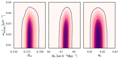
Figure 7: The two-dimensional likelihoods of $m_{\textsc{wdm}}^{-1},\Omega_{M},H_{0}$ and $\sigma_{8}$ that illustrate the correlation between these parameters. Each plot shows a 2-dimensional slice of the likelihood while keeping all other parameters to their true value. The colors represent the value of likelihood and the contour lines shows 68% and 95% credible levels. It can be seen that there is no correlation between $m_{\textsc{wdm}}^{-1}$ and the cosmological parameters.

We also check whether the change in the expected number of strongly lensed events and their time delay distribution due to differences in the DM models could be mimicked by changes in cosmological parameters as studied in Jana et al. (2023, 2024). If such a degeneracy exists, the properties of the DM particle will be indistinguishable from cosmological parameters. To study this, we generate a sample of lensed BBH events assuming the standard value of the cosmological parameters that we used in the paper along with the CDM HMF. We then compute the likelihood by simultaneously varying $m_{\textsc{wdm}}$ as well as the cosmological parameters $H_{0},\Omega_{M}$ and $\sigma_{8}$. Figure 7 shows various 2-dimensional slices of the likelihood that illustrate the lack of correlation between $m_{\textsc{wdm}}$ and cosmological parameters. This suggests that marginalising over the cosmological parameters will not change the posterior of $m_{\textsc{wdm}}^{-1}$ significantly. We leave a joint analysis including $m_{\textsc{wdm}}^{-1}$ and all other cosmological parameters for future work.

The effect of WDM that we consider is the suppression in the number density of low mass halos. Besides this effect, WDM predicts the existence of finite central cores in DM halos Tremaine and Gunn (1979); Bode et al. (2001), as opposed to the cuspy profile expected in CDM. The presence of a central core reduces the Einstein angle of the lens, resulting in smaller time delays as compared to halos without core. This effect can be populate the low-time delay part of the time-delay distribution, potentially mimicking CDM halos. However, the presence of cores will also reduce the lensing optical depth. Our preliminary investigations suggest that the resulting reduction in the number of lensed events should make them distinguishable from the CDM halos. This is being investigated in a follow-up work.

Summary and Outlook:—

The large number of strongly lensed GW signals detectable by the XG detectors will enable new probes of cosmology. In this letter, we showed how the expected number of strongly lensed BBH mergers and the distribution of the time delay between lensed images can be used to constrain the nature of particle DM. In particular, the suppression of the low-mass DM halos predicted by the WDM/FDM models will result in a reduction in the number of strongly lensed GW signals with small lensing time delays. This will allow us to constrain the mass of the WDM/FDM particle. The expected constraints are significantly better than the current bounds. In the time delay distribution, there is no degeneracy between the nature of DM particle and the cosmological parameters. This should allow us to constrain both the nature of DM and cosmological parameters simultaneously from future observations.

Because of their inherent simplicity, GWs are unaffected by extinction, and selection effects in GW searches are well modelled. This makes GW strong lensing a cleaner probe than, e.g., optical lensing. However, a number of obstacles need to be addressed before this technique can be applied to constrain the nature of DM. The properties of astrophysical sources and lenses determine both the number of lensed events and the distribution of their time delays. Some of the relevant parameters, such as the redshift distribution of BBH mergers, can be inferred from the large number of unlensed GW signals as well as the stochastic GW background. For other parameters, such as the distribution of the properties of the lens parameters, will need to rely on models obtained from large-scale cosmological simulations and galaxy surveys.

In this letter, we have assumed that the lenses are modelled by simple SISs, whose parameters are obtained from the HMF using a simple prescription. We also neglected the halo sub structure and the effect of baryons. Future analysis needs to model the lenses more accurately, which are working on improving Jana et al. . We neglected selection function of the detectors assuming that XG detectors will observe all the BBHs out to large redshifts. In order to forecast the expected constraints from the upcoming upgrades of the current generation detectors Fritschel et al. (2024); Adhikari et al. (2024, 2020), we will need to take into account the selection effects also, which is being studied in another ongoing work Maity et al. (a). There are other potential sources of systematics: The false positives produced by the methods used to identify strongly lensed signals can contaminate our observational sample and can bias the parameter inference. In Jana et al. (2024) we demonstrated how we can model the contamination thus evading systematic biases in the estimation of cosmological parameters from strongly lensed GW signals. A similar approach can be adopted here as well.

While we have focussed on BBH signals, strongly lensed binary neutron star mergers, which are expected to be equally abundant Baibhav et al. (2019); Magare et al. (2023); Smith et al. (2023), could also be used to probe cosmological parameters and the nature of DM. In contrast to BBH mergers which can be observed out to very large redshifts ($z\sim 10$), neutron star mergers can be observed out to smaller redshifts ($z\sim 1$) even using XG detectors. However, some of them would have an electromagnetic counterpart which will also be lensed. Such observations could allow us to probe the detailed profile of the lensing galaxy, potentially enabling to put tighter constraints on the nature of DM. This is being explored in an ongoing work Maity et al. (b).

I Bayesian inference

We assume that we have confidently detected $N$ strongly lensed BBH events within an observation period of $T_{\mathrm{obs}}$, each producing two observable copies (lensed images). We aim to compute the posterior distribution of the mass $m_{\textsc{wdm}}$ of the WDM particle, using the time delays $\left\{\Delta t_{i}\right\}_{i=1}^{N}$ from the $N$ detected lensed events.

We can write the likelihood $p\left(N,\left\{\Delta t_{i}\right\}~{}\big{|}~{}m_{\textsc{wdm}}^{-1},T_{\mathrm{obs}}\right)$ as a product of two likelihoods as $N$ and $\left\{\Delta t_{i}\right\}$ are uncorrelated. The likelihood of observing $N$ events can be described as a Poisson distribution

$$p\left(N~{}\big{|}~{}m_{\textsc{wdm}}^{-1},T_{\mathrm{obs}}\right)=\frac{\Lambda\left(m_{\textsc{wdm}}^{-1}\right)^{N}e^{-\Lambda\left(m_{\textsc{wdm}}^{-1}\right)}}{N!},$$ (1)

where $\Lambda\left(m_{\textsc{wdm}}^{-1}\right)$ is the expected number of lensed events for a given value of $m_{\textsc{wdm}}^{-1}$. The likelihood of observing a set of time delays $\left\{\Delta t_{i}\right\}$ can be written as

$$p\left(\left\{\Delta t_{i}\right\}~{}\big{|}~{}m_{\textsc{wdm}}^{-1},T_{\mathrm{obs}}\right)=\prod_{i=1}^{N}p\left(\Delta t_{i}~{}\big{|}~{}m_{\textsc{wdm}}^{-1},T_{\mathrm{obs}}\right).$$ (2)

Here we assume each BBH merger to be an independent event and that the time delays are measured accurately and precisely. $p\left(\Delta t_{i}~{}\big{|}~{}m_{\textsc{wdm}}^{-1},T_{\mathrm{obs}}\right)$ is the “model” time delay distribution calculated at measured time delay $\Delta t_{i}$. The model time delay distribution is calculated from the expected time delay distribution $p\left(\left\{\Delta t_{i}\right\}~{}\big{|}~{}m_{\textsc{wdm}}^{-1}\right)$, considering the fact that time delays greater than the observation time period $T_{\mathrm{obs}}$ cannot be observed, see Jana et al. (2023, 2024) for more details. Evaluation of the likelihood, $p\left(N,\left\{\Delta t_{i}\right\}~{}\big{|}~{}m_{\textsc{wdm}}^{-1},T_{\mathrm{obs}}\right)$ requires the expected number of lensed events, $\Lambda$ and expected time delay distribution, $p\left(\left\{\Delta t_{i}\right\}~{}\big{|}~{}m_{\textsc{wdm}}^{-1}\right)$ for different values of $m_{\textsc{wdm}}^{-1}$. These quantities depend on the values of cosmological parameters and the distribution of the source and lens properties Jana et al. (2023, 2024). Here we fix the cosmological parameters to the Planck values, $\vec{\Omega}_{P}=\{\Omega_{m}=0.316,H_{0}=67.3,\sigma_{8}=0.816\}$Aghanim et al. (2020). We also consider the distribution of source and lens properties is obtained by other observations, theoretical studies and large scale cosmological simulations.

II Calculation of expected number of lensed events and time delay distribution

We calculate the expected number of lensed events $\Lambda\left(m_{\textsc{wdm}}^{-1},T_{\mathrm{obs}}\right)$ and the expected time delay distribution $p\left(\Delta t~{}\big{|}~{}m_{\textsc{wdm}}^{-1}\right)$ using equations 7 and 17 of Jana et al. (2024). The expected number of lensed events and their time delay distribution depends on $m_{\textsc{wdm}}^{-1}$ through the halo mass function. All the assumptions and inputs (source and lens distributions), used to calculate the total number of lensed events and their time delay distribution are same as outlined in Jana et al. (2023). We assume that the source redshift distribution, $p_{b}(z_{s})$ will be known with adequate precision from the observation form unlensed events which will dominate the future dataset. For illustration, we use the source redshift distribution provided by the source population model Dominik et al. (2013), assuming standard cosmology, $\vec{\Omega_{p}}$. We model the distribution of lenses using the halo mass function, which gives the distribution, $p\left(\sigma,z_{\ell}\right)$ of $\sigma$ and $z_{\ell}$. We consider a mass range of $10^{8}$ to $10^{15}\;M_{\odot}$ for the lenses. For further details on the calculations, refer to Jana et al. (2023, 2024) and for insights into how the time delay distributions and the total number of lensed events are affected by changes in the assumptions about source population and lens distributions, please refer to Jana et al. (2024). We consider halo mass function model described in Behroozi et al. (2013). To check the bias incurred in the inference on the $m_{\textsc{wdm}}^{-1}$ by using wrong model of halo mass function we also consider another model of halo mass function described by Jenkins et al. (2001).

References

- Behroozi et al. (2013) P. S. Behroozi, R. H. Wechsler, and C. Conroy, ApJ 770, 57 (2013), arXiv:1207.6105 [astro-ph.CO] .
- Jenkins et al. (2001) A. Jenkins, C. Frenk, S. D. White, J. M. Colberg, S. Cole, A. E. Evrard, H. Couchman, and N. Yoshida, Monthly Notices of the Royal Astronomical Society 321, 372 (2001).
- Bertone and Hooper (2018) G. Bertone and D. Hooper, Rev. Mod. Phys. 90, 045002 (2018).
- Arbey and Mahmoudi (2021) A. Arbey and F. Mahmoudi, Progress in Particle and Nuclear Physics 119, 103865 (2021).
- Carr and Kühnel (2022) B. Carr and F. Kühnel, SciPost Physics Lecture Notes (2022), 10.21468/scipostphyslectnotes.48.
- Griest and Kamionkowski (2000) K. Griest and M. Kamionkowski, Physics Reports 333-334, 167 (2000).
- Feng (2010) J. L. Feng, Annual Review of Astronomy and Astrophysics 48, 495 (2010), https://doi.org/10.1146/annurev-astro-082708-101659 .
- Green and Kavanagh (2021) A. M. Green and B. J. Kavanagh, Journal of Physics G: Nuclear and Particle Physics 48, 043001 (2021).
- White et al. (1983) S. D. M. White, C. S. Frenk, and M. Davis, ApJ 274, L1 (1983).
- Kawasaki et al. (1997) M. Kawasaki, N. Sugiyama, and T. Yanagida, Modern Physics Letters A 12, 1275 (1997), https://doi.org/10.1142/S021773239700128X .
- Boyarsky et al. (2019) A. Boyarsky, M. Drewes, T. Lasserre, S. Mertens, and O. Ruchayskiy, Progress in Particle and Nuclear Physics 104, 1 (2019).
- Komatsu et al. (2011) E. Komatsu, K. M. Smith, J. Dunkley, C. L. Bennett, B. Gold, G. Hinshaw, N. Jarosik, D. Larson, M. R. Nolta, L. Page, D. N. Spergel, M. Halpern, R. S. Hill, A. Kogut, M. Limon, S. S. Meyer, N. Odegard, G. S. Tucker, J. L. Weiland, E. Wollack, and E. L. Wright, The Astrophysical Journal Supplement Series 192, 18 (2011).
- Cole et al. (2005) S. Cole, W. J. Percival, J. A. Peacock, P. Norberg, C. M. Baugh, C. S. Frenk, I. Baldry, J. Bland-Hawthorn, T. Bridges, R. Cannon, M. Colless, C. Collins, W. Couch, N. J. G. Cross, G. Dalton, V. R. Eke, R. de Propris, S. P. Driver, G. Efstathiou, R. S. Ellis, K. Glazebrook, C. Jackson, A. Jenkins, O. Lahav, I. Lewis, S. Lumsden, S. Maddox, D. Madgwick, B. A. Peterson, W. Sutherland, K. Taylor, and T. 2dFGRS Team, Monthly Notices of the Royal Astronomical Society 362, 505 (2005), https://academic.oup.com/mnras/article-pdf/362/2/505/6155670/362-2-505.pdf .
- Tegmark et al. (2006) M. Tegmark, D. J. Eisenstein, M. A. Strauss, D. H. Weinberg, M. R. Blanton, J. A. Frieman, M. Fukugita, J. E. Gunn, A. J. S. Hamilton, G. R. Knapp, R. C. Nichol, J. P. Ostriker, N. Padmanabhan, W. J. Percival, D. J. Schlegel, D. P. Schneider, R. Scoccimarro, U. c. v. Seljak, H.-J. Seo, M. Swanson, A. S. Szalay, M. S. Vogeley, J. Yoo, I. Zehavi, K. Abazajian, S. F. Anderson, J. Annis, N. A. Bahcall, B. Bassett, A. Berlind, J. Brinkmann, T. Budavari, F. Castander, A. Connolly, I. Csabai, M. Doi, D. P. Finkbeiner, B. Gillespie, K. Glazebrook, G. S. Hennessy, D. W. Hogg, i. c. v. Ivezić, B. Jain, D. Johnston, S. Kent, D. Q. Lamb, B. C. Lee, H. Lin, J. Loveday, R. H. Lupton, J. A. Munn, K. Pan, C. Park, J. Peoples, J. R. Pier, A. Pope, M. Richmond, C. Rockosi, R. Scranton, R. K. Sheth, A. Stebbins, C. Stoughton, I. Szapudi, D. L. Tucker, D. E. V. Berk, B. Yanny, and D. G. York, Phys. Rev. D 74, 123507 (2006).
- Kauffmann et al. (1993) G. Kauffmann, S. D. M. White, and B. Guiderdoni, Monthly Notices of the Royal Astronomical Society 264, 201 (1993), https://academic.oup.com/mnras/article-pdf/264/1/201/3734439/mnras264-0201.pdf .
- Klypin et al. (1999) A. Klypin, A. V. Kravtsov, O. Valenzuela, and F. Prada, The Astrophysical Journal 522, 82 (1999).
- Moore et al. (1999) B. Moore, S. Ghigna, F. Governato, G. Lake, T. Quinn, J. Stadel, and P. Tozzi, The Astrophysical Journal 524, L19 (1999).
- Bode et al. (2001) P. Bode, J. P. Ostriker, and N. Turok, 556, 93 (2001).
- Kim et al. (2018) S. Y. Kim, A. H. G. Peter, and J. R. Hargis, Phys. Rev. Lett. 121, 211302 (2018), arXiv:1711.06267 [astro-ph.CO] .
- de Blok (2010) W. J. G. de Blok, Advances in Astronomy 2010, 1–14 (2010).
- Spergel and Steinhardt (2000) D. N. Spergel and P. J. Steinhardt, Physical Review Letters 84, 3760–3763 (2000).
- Hu et al. (2000) W. Hu, R. Barkana, and A. Gruzinov, Physical Review Letters 85, 1158–1161 (2000).
- Viel et al. (2013) M. Viel, G. D. Becker, J. S. Bolton, and M. G. Haehnelt, Phys. Rev. D 88, 043502 (2013).
- Markovič and Viel (2014) K. Markovič and M. Viel, Publications of the Astronomical Society of Australia 31, e006 (2014).
- Yèche et al. (2017) C. Yèche, N. Palanque-Delabrouille, J. Baur, and H. du Mas des Bourboux, Journal of Cosmology and Astroparticle Physics 2017, 047 (2017).
- Villasenor et al. (2023) B. Villasenor, B. Robertson, P. Madau, and E. Schneider, Phys. Rev. D 108, 023502 (2023).
- Vegetti et al. (2023) S. Vegetti, S. Birrer, G. Despali, C. D. Fassnacht, D. Gilman, Y. Hezaveh, L. P. Levasseur, J. P. McKean, D. M. Powell, C. M. O’Riordan, and G. Vernardos, “Strong gravitational lensing as a probe of dark matter,” (2023), arXiv:2306.11781 [astro-ph.CO] .
- Enzi et al. (2021) W. Enzi, R. Murgia, O. Newton, S. Vegetti, C. Frenk, M. Viel, M. Cautun, C. D. Fassnacht, M. Auger, G. Despali, J. McKean, L. V. E. Koopmans, and M. Lovell, Monthly Notices of the Royal Astronomical Society 506, 5848 (2021), https://academic.oup.com/mnras/article-pdf/506/4/5848/39729079/stab1960.pdf .
- Bozek et al. (2015) B. Bozek, D. J. E. Marsh, J. Silk, and R. F. G. Wyse, Monthly Notices of the Royal Astronomical Society 450, 209 (2015), https://academic.oup.com/mnras/article-pdf/450/1/209/18503963/stv624.pdf .
- Schive et al. (2016) H.-Y. Schive, T. Chiueh, T. Broadhurst, and K.-W. Huang, The Astrophysical Journal 818, 89 (2016).
- Corasaniti et al. (2017) P. S. Corasaniti, S. Agarwal, D. J. E. Marsh, and S. Das, Phys. Rev. D 95, 083512 (2017).
- Iršič et al. (2017) V. Iršič, M. Viel, M. G. Haehnelt, J. S. Bolton, and G. D. Becker, Phys. Rev. Lett. 119, 031302 (2017).
- Marsh and Niemeyer (2019) D. J. E. Marsh and J. C. Niemeyer, Phys. Rev. Lett. 123, 051103 (2019).
- Bertone et al. (2019) G. Bertone, D. Croon, M. A. Amin, K. K. Boddy, B. J. Kavanagh, K. J. Mack, P. Natarajan, T. Opferkuch, K. Schutz, V. Takhistov, C. Weniger, and T.-T. Yu, arXiv e-prints , arXiv:1907.10610 (2019), arXiv:1907.10610 [astro-ph.CO] .
- Amaro-Seoane and et al. (2017) P. Amaro-Seoane and H. A. et al., “Laser interferometer space antenna,” (2017), arXiv:1702.00786 [astro-ph.IM] .
- Kavanagh et al. (2020) B. J. Kavanagh, D. A. Nichols, G. Bertone, and D. Gaggero, Phys. Rev. D 102, 083006 (2020).
- Kadota et al. (2023) K. Kadota, J. H. Kim, P. Ko, and X.-Y. Yang, “Gravitational wave probes on self-interacting dark matter surrounding an intermediate mass black hole,” (2023), arXiv:2306.10828 [hep-ph] .
- Richard et al. (2015) B. Richard, C. Vitor, and P. Paolo, (2015), https://doi.org/10.1007/978-3-319-19000-6.
- Arvanitaki and Dubovsky (2011) A. Arvanitaki and S. Dubovsky, Phys. Rev. D 83, 044026 (2011).
- Arvanitaki et al. (2015) A. Arvanitaki, M. Baryakhtar, and X. Huang, Phys. Rev. D 91, 084011 (2015).
- Brito et al. (2017) R. Brito, S. Ghosh, E. Barausse, E. Berti, V. Cardoso, I. Dvorkin, A. Klein, and P. Pani, Phys. Rev. D 96, 064050 (2017).
- Baryakhtar et al. (2017) M. Baryakhtar, R. Lasenby, and M. Teo, Phys. Rev. D 96, 035019 (2017).
- Porayko et al. (2018) N. K. Porayko, X. Zhu, Y. Levin, L. Hui, et al. (PPTA Collaboration), Phys. Rev. D 98, 102002 (2018).
- Dai et al. (2018) L. Dai, S.-S. Li, B. Zackay, S. Mao, and Y. Lu, Phys. Rev. D 98, 104029 (2018).
- Oguri and Takahashi (2020) M. Oguri and R. Takahashi, The Astrophysical Journal 901, 58 (2020).
- Choi et al. (2021) H. G. Choi, C. Park, and S. Jung, Phys. Rev. D 104, 063001 (2021).
- Gao et al. (2022) Z. Gao, X. Chen, Y.-M. Hu, J.-D. Zhang, and S.-J. Huang, Monthly Notices of the Royal Astronomical Society 512, 1 (2022), https://academic.oup.com/mnras/article-pdf/512/1/1/42857662/stac365.pdf .
- Guo and Lu (2022) X. Guo and Y. Lu, Phys. Rev. D 106, 023018 (2022).
- Çalışkan et al. (2023) M. Çalışkan, N. A. Kumar, L. Ji, J. M. Ezquiaga, R. Cotesta, E. Berti, and M. Kamionkowski, “Probing wave-optics effects and dark-matter subhalos with lensing of gravitational waves from massive black holes,” (2023), arXiv:2307.06990 [astro-ph.CO] .
- Cao et al. (2020) S. Cao, J. Qi, M. Biesiada, T. Liu, J. Li, and Z.-H. Zhu, Monthly Notices of the Royal Astronomical Society: Letters 502, L16 (2020), https://academic.oup.com/mnrasl/article-pdf/502/1/L16/35871916/slaa205.pdf .
- Cao, Shuo et al. (2022) Cao, Shuo, Qi, Jingzhao, Cao, Zhoujian, Biesiada, Marek, Cheng, Wei, and Zhu, Zong-Hong, A&A 659, L5 (2022).
- Hall and Evans (2019) E. D. Hall and M. Evans, Classical and Quantum Gravity 36, 225002 (2019).
- Xu et al. (2022) F. Xu, J. M. Ezquiaga, and D. E. Holz, Astrophys. J. 929, 9 (2022), arXiv:2105.14390 [astro-ph.CO] .
- Jana et al. (2023) S. Jana, S. J. Kapadia, T. Venumadhav, and P. Ajith, Phys. Rev. Lett. 130, 261401 (2023).
- Haris et al. (2018) K. Haris, A. K. Mehta, S. Kumar, T. Venumadhav, and P. Ajith, arXiv e-prints , arXiv:1807.07062 (2018), arXiv:1807.07062 [gr-qc] .
- Li et al. (2018) S.-S. Li, S. Mao, Y. Zhao, and Y. Lu, Mon. Not. Roy. Astron. Soc. 476, 2220 (2018), arXiv:1802.05089 [astro-ph.CO] .
- Mukherjee et al. (2021) S. Mukherjee, T. Broadhurst, J. M. Diego, J. Silk, and G. F. Smoot, Mon. Not. Roy. Astron. Soc. 506, 3751 (2021), arXiv:2106.00392 [gr-qc] .
- Robertson et al. (2020) A. Robertson, G. P. Smith, R. Massey, V. Eke, M. Jauzac, M. Bianconi, and D. Ryczanowski, MNRAS 495, 3727 (2020), arXiv:2002.01479 [astro-ph.CO] .
- Janquart et al. (2022) J. Janquart, A. More, and C. Van Den Broeck, arXiv e-prints , arXiv:2205.11499 (2022), arXiv:2205.11499 [gr-qc] .
- More and More (2022) A. More and S. More, Mon. Not. Roy. Astron. Soc. 515, 1044 (2022), arXiv:2111.03091 [astro-ph.CO] .
- Maggiore et al. (2020) M. Maggiore, C. Van Den Broeck, N. Bartolo, E. Belgacem, D. Bertacca, M. A. Bizouard, M. Branchesi, S. Clesse, S. Foffa, J. García-Bellido, et al., Journal of Cosmology and Astroparticle Physics 2020, 050 (2020).
- Reitze et al. (2019) D. Reitze, R. X. Adhikari, S. Ballmer, B. Barish, L. Barsotti, G. Billingsley, D. A. Brown, Y. Chen, D. Coyne, R. Eisenstein, M. Evans, P. Fritschel, E. D. Hall, A. Lazzarini, G. Lovelace, J. Read, B. S. Sathyaprakash, D. Shoemaker, J. Smith, C. Torrie, S. Vitale, R. Weiss, C. Wipf, and M. Zucker, in Bulletin of the American Astronomical Society, Vol. 51 (2019) p. 35, arXiv:1907.04833 [astro-ph.IM] .
- Bardeen et al. (1986) J. M. Bardeen, J. R. Bond, N. Kaiser, and A. S. Szalay, ApJ 304, 15 (1986).
- Viel et al. (2005) M. Viel, J. Lesgourgues, M. G. Haehnelt, S. Matarrese, and A. Riotto, Phys. Rev. D 71, 063534 (2005).
- Schneider et al. (2012) A. Schneider, R. E. Smith, A. V. Macciò, and B. Moore, Monthly Notices of the Royal Astronomical Society 424, 684 (2012), https://academic.oup.com/mnras/article-pdf/424/1/684/3296247/mnras0424-0684.pdf .
- Murray et al. (2013) S. G. Murray, C. Power, and A. S. G. Robotham, Astronomy and Computing 3, 23 (2013), arXiv:1306.6721 [astro-ph.CO] .
- Peter Schneider (1999) E. E. F. Peter Schneider, Jürgen Ehlers, (1999), https://doi.org/10.1007/978-3-662-03758-4.
- Dominik et al. (2013) M. Dominik, K. Belczynski, C. Fryer, D. E. Holz, E. Berti, T. Bulik, I. Mandel, and R. O’Shaughnessy, The Astrophysical Journal 779, 72 (2013).
- Aghanim et al. (2020) N. Aghanim, Y. Akrami, M. Ashdown, J. Aumont, C. Baccigalupi, M. Ballardini, A. Banday, R. Barreiro, N. Bartolo, S. Basak, et al., Astronomy & Astrophysics 641, A6 (2020).
- Jana et al. (2024) S. Jana, S. J. Kapadia, T. Venumadhav, S. More, and P. Ajith, “Strong-lensing cosmography using third-generation gravitational-wave detectors,” (2024), arXiv:2405.17805 .
- Tremaine and Gunn (1979) S. Tremaine and J. E. Gunn, Phys. Rev. Lett. 42, 407 (1979).
- (72) S. Jana, S. J. Kapadia, T. Venumadhav, S. More, and P. Ajith, “Effect of lens models on strong lensing cosmography using gravitational waves,” .
- Fritschel et al. (2024) P. Fritschel, K. Kuns, J. Driggers, et al., LIGO-T2200287-v3 (2024).
- Adhikari et al. (2024) R. X. Adhikari, K. Arai, A. Brooks, et al., LIGO-M2300123 (2024).
- Adhikari et al. (2020) R. X. Adhikari, K. Arai, A. F. Brooks, C. Wipf, O. Aguiar, et al., Classical and Quantum Gravity 37, 165003 (2020).
- Maity et al. (a) K. N. Maity, S. Jana, S. J. Kapadia, T. Venumadhav, S. More, and P. Ajith, “Strong-lensing cosmography using upgraded second-generation gravitational-wave detectors,” (a).
- Baibhav et al. (2019) V. Baibhav, E. Berti, D. Gerosa, M. Mapelli, N. Giacobbo, Y. Bouffanais, and U. N. Di Carlo, Phys. Rev. D 100, 064060 (2019).
- Magare et al. (2023) S. Magare, S. J. Kapadia, A. More, M. K. Singh, P. Ajith, and A. N. Ramprakash, “Gear-up for the action replay: Leveraging lensing for enhanced gravitational-wave early-warning,” (2023), arXiv:2302.02916 [astro-ph.HE] .
- Smith et al. (2023) G. P. Smith, A. Robertson, G. Mahler, M. Nicholl, D. Ryczanowski, M. Bianconi, K. Sharon, R. Massey, J. Richard, and M. Jauzac, Monthly Notices of the Royal Astronomical Society 520, 702–721 (2023).
- Maity et al. (b) K. N. Maity, S. Jana, U. Deka, and P. Ajith, “Constraining dark matter substructure using multi-messenger observations of binary neutron star mergers,” (b).
Supplemental Material: