Can a Bayesian Oracle Prevent Harm from an Agent?
Abstract
Is there a way to design powerful AI systems based on machine learning methods that would satisfy probabilistic safety guarantees? With the long-term goal of obtaining a probabilistic guarantee that would apply in every context, we consider estimating a context-dependent bound on the probability of violating a given safety specification. Such a risk evaluation would need to be performed at run-time to provide a guardrail against dangerous actions of an AI. Noting that different plausible hypotheses about the world could produce very different outcomes, and because we do not know which one is right, we derive bounds on the safety violation probability predicted under the true but unknown hypothesis. Such bounds could be used to reject potentially dangerous actions. Our main results involve searching for cautious but plausible hypotheses, obtained by a maximization that involves Bayesian posteriors over hypotheses. We consider two forms of this result, in the i.i.d. case and in the non-i.i.d. case, and conclude with open problems towards turning such theoretical results into practical AI guardrails.
1 Introduction
Ensuring that an AI system will not misbehave is a challenging open problem [4], particularly in the current context of rapid growth in AI capabilities. Governance measures and evaluation-based strategies have been proposed to mitigate the risk of harm from highly capable AI systems, but do not provide any form of safety guarantee when no undesired behavior is detected. In contrast, the safe-by-design paradigm involves designing AI systems with quantitative (possibly probabilistic) safety guarantees from the ground up, and therefore could represent a stronger form of protection [8]. However, how to design such systems remains an open problem too.
Since testing an AI system for violations of a safety specification in every possible context, e.g., every (query, output) pair, is impossible, we consider a rejection sampling approach that declines a candidate output or action if it has a probability of violating a given safety specification that is too high. The question of defining the safety specification (the violation of which is simply referred to as “harm” below) is important and left to future work, possibly following up approaches such as constitutional AI [1]. We also note that being Bayesian about the interpretation of a human-specified safety specification would protect against the AI wrongly believing an incorrect interpretation. Here we instead focus on a question inspired by risk-management practice [24]: even though the true probability of harm following from some proposed action is unknown, because the true data-generating process is unknown, can we bound that risk using quantities that can be estimated by machine learning methods given the observed data?
To illustrate this question, consider a committee of “wise” humans whose theories about the world are all equally compatible with the available data, knowing that an unknown member of the committee has the correct theory. Each committee member can make a prediction about the probability of future harm that would result from following some action in some context. Marginalizing this harm probability over the committee members amounts to making them vote with equal weights. If the majority is aligned with the correct member’s prediction, then all is good, i.e., if the correct theory predicts harm, then the committee will predict harm and can choose to avoid the harmful action. But what if the correct member is in the minority regarding their harm prediction? To get a guarantee that the true harm probability is below a given threshold, we could simply consider the committee member whose theory predicts the highest harm probability and we would be sure that their harm probability prediction upper bounds the true harm probability. In practice, we do not get equally “wise” committee members, so we can correct this calculation based on how plausible the theory harbored by each committee member is. In a Bayesian framework, the plausibility of a theory corresponds to its posterior over all theories given the observed data, which is proportional to the data likelihood given the theory times the prior probability of that theory.
In this paper, we show how results about posterior consistency can provide probabilistic risk bounds. All the results have the form of inequalities, where the true probability of harm is upper bounded by a quantity that can in principle be estimated, given enough computational resources to approximate Bayesian posteriors over theories given the provided data. In addition, these are not hard bounds but only hold with some probability, and there is generally a trade-off between that probability and the tightness of the bound. We study two scenarios in the corresponding sections: the i.i.d. data setting in Section 3 and the non-i.i.d. data setting in Section 4. In all cases, a key intermediate result is a bound relating the Bayesian posterior on the unknown true theory and the probability of other theories (with propositions labeled True theory dominance). The idea is that because the true theory generated the data, its posterior tends to increase as more data is acquired, and in the i.i.d. case it comes to dominate other theories. From such a relationship, the harm risk bound can be derived with very little algebra (yielding propositions labeled Harm probability bound).
We conclude this paper with a discussion of open problems that should be considered in order to turn such bounds into a safe-by-design AI system, taking into account the challenge of representing the notion of harm and reliable conditional probabilities, as well as the fact that, in general, the estimation of the required conditional probabilities will be imperfect.
2 Safe-by-design AI?
Before an AI is built and deployed, it is important that the developers have high assurances that the AI will behave well. Dalrymple et al. [8] propose an approach to “guaranteed safe AI” designs with built-in high-assurance quantitative safety guarantees, although these guarantees can sometimes be probabilistic and only asymptotic. It remains an open question whether and how that research program can be realized. The authors take existing examples of quantitative guarantees in safety-critical systems and motivate why such a framework should be adopted if we ever build AI systems that match or exceed human cognitive abilities and could potentially act in dangerous ways. Their program is motivated by current known limitations of state-of-the-art AI systems based on deep learning, including the challenge of engineering AI systems that robustly act as intended [7, 22, 27, 28, 44, 33, 34, 19, 32].
The approach proposed by [8] has the following components: a world model (which can be a distribution about hypotheses explaining the data), a safety specification (what are considered unacceptable states of the world), and a verifier (a computable procedure that checks whether a policy or action violates the safety specification).
Here, we study elements that would go into such a safe-by-design AI system. We assume that the system infers a probabilistic world model, or theory, and updates its estimate of , via machine learning, using the stream of observed data . The observations are assumed to come from a data-generating process given by a ground-truth world model , which lies in the system’s space of possible theories.
The inference of the theory is Bayesian, meaning that the system maintains an estimate of the posterior over theories, , where is proportional to the product of the prior probability with the likelihood of the observations under the theory, . In the simplest case, is a point estimate, which would optimally place its mass on the mode of the posterior. Inference of the latent theory allows the system to approximate conditional probabilities over any random variables known to the world model.
The safety specification is assumed to be given in the form of a binary random variable (which we call “harm” below) whose probability given the other variables may depend on the theory . We are interested in predicting the probability of harm under the true theory . Because is unknown, we propose to estimate upper bounds on this probability using the estimated posteriors. These upper bounds can be used as thresholds for a verifier that checks whether the risk of harm falls below some acceptable level.
Following Dalrymple et al. [8], we assume that the notion of harm has been specified, possibly in natural language, and that the ambiguities about its interpretation are represented within the Bayesian posterior . This paper focuses on the verifier, under different assumptions of i.i.d. or non-i.i.d. data.
What do the observations and context represent?
We give a possible interpretation of the objects introduced in the preceding discussion in the simple case of an agent acting in a fully observed environment (MDP), where the theory is a transition model and the occurrence of harm at a state is conditionally independent of all other variables given .
-
•
Observations are observed transitions , where is a state, is an action, and is the next state.
-
•
Theories encode the state visitation and transition probabilities; in particular, conditioning on gives transition probabilities . (In the i.i.d. setting, the state visitation distribution would have to be stationary.)
-
•
The dataset is a set of observed transitions.
-
•
The context variable is a pair , where is a state and is an action being considered at state .
-
•
The harm probability can be any function of the theory , the context , and the data . For example, this probability could be derived from a fixed specification of what it means for a state to be harmful, . Then, the harm probability could be computed as .
We note that the interpretation of harm probability in the example above includes the case where the occurrence of harm is an observed variable that is part of the state : in that case, one sets if is harmful (), and otherwise. Then the harm probability is just the probability, under , of reaching a harmful state, and observations of harm in affect the Bayesian posterior over theories.
This interpretation also includes the case where the harm probability is a function of the state , but occurrence or nonoccurrence of harm is not observed in . For example, a language model encoding world knowledge and human preferences or constraints, or an iterative reasoning procedure that uses those constraints, could generate some specification of harm , although perhaps unreliably.
Finally, a setting that separates the predicted next state from the harm variable in this way gives a framework for studying how an agent might tamper with harm guardrails. If the state decomposes as , and is deterministic as a function of , except for some difficult-to-reach values of , then the agent can try to reach those values of , so that harm is ‘recorded’ as not having occurred, even though it has. We discuss this briefly at the end of Section 4.
3 I.I.D. data
Following the notation introduced in the previous section, here we consider the easier-to-analyze case where the observed examples are sampled i.i.d. from the unknown distribution . Assuming that the set of theories assigns a nonzero prior mass to , and all theories are distinct distributions, it can be shown that the posterior converges to a point mass at . It follows that for sufficiently large , we can bound the probability under of an event (e.g., harm) given conditions (e.g., an action and a context) by looking at the probability of given and under a plausible but cautious theory that maximizes .
Setting.
Fix a complete separable metric space , called the observation space, let be its Borel -algebra, and fix a -finite measure on . A theory is a probability distribution (measure) on the measurable space that is absolutely continuous w.r.t. . If is a theory, we denote by the Radon-Nikodym derivative , which is uniquely defined up to -a.e. equality. Any theory also canonically determines a -valued random variable by the identity map on the probability space .
One can keep in mind two cases:
-
(1)
is a finite or countable set and is the counting measure. Theories are equivalent to probability mass functions .
-
(2)
and is the Lebesgue measure. Theories are equivalent to their probability density functions up to a.e. equality.
Consider a countable (possibly finite) set of theories containing a ground truth theory and fix a choice of a (measurable) density function for each .
Definition of posterior as a random variable.
If is a prior distribution111To be precise, is endowed with the counting measure and we flexibly interchange distributions and mass functions on . on and , we define the posterior to be the distribution with mass function
| (1) |
assuming the denominator converges and the sum is nonzero. Otherwise, the posterior is considered to be undefined. As written, the posterior depends on the choice of density functions , but any two that are -a.e. equal yield the same posterior for -a.e. .
For , we write for the posterior given observation and prior , and similarly for a longer sequence of observations. It can be checked that is invariant to the order of and that it is defined in one order if and only if it is defined in all orders. This allows us to unambiguously write where is a finite multiset of observations, and we have
| (2) |
Let be the ground truth theory and a prior over . Consider a sequence of i.i.d. -valued random variables (whose realizations are the observations), where each follows the distribution . For any , the posterior is then a random variable taking values in the space of probability mass functions on .222To be precise, the random variable has domain and codomain the space of functions summing to 1. The function taking a sequence of observations in to the posterior probability mass function is measurable, which follows from each being measurable in and elementary facts.
Bayesian posterior consistency.
We recall and state in our setting a result about the concentration of the posterior at the ground truth theory as the number of observations increases.
Proposition 3.1 (True theory dominance).
Under the above conditions and supposing that , the posterior is almost surely defined for all , and the following almost surely hold:
-
(a)
as measures; equivalently, .
-
(b)
There exists such that for all .
Proof.
This is an application of Doob’s posterior consistency theorem ([12]; see also [25] for a modern summary). This result, which follows from the theory of martingales, assumes that is sampled from the prior distribution and the observations are defined as above. Doob’s theorem states that if for every , the map is measurable, then the posteriors are almost surely defined and (a) holds -almost surely with respect to the choice of .
In our case, because is countable, the measurability condition is satisfied, showing that (a) holds for -almost every . In particular, if , then (a) holds.
Finally, by (a), we have that for any , there exists such that for every , , or, equivalently, , and therefore for all . In particular, taking , we get that for sufficiently large , for every , which shows (b). ∎
Note that this result assumes that all theories in are distinct as probability measures (so no two of the are -a.e. equal).
On necessity of conditions.
The i.i.d. assumption in Proposition 3.1 is necessary; see Remark 4.3 for an example where does not almost surely approach 1.
Remark 3.2.
The assumption that the data-generating process lies in and has positive prior mass is also necessary for convergence of the posterior. To illustrate this, we give a simple example in which the theories are Bernoulli distributions and the posterior does not converge to any distribution over .
Take and for some , where . Assume a prior with and take the true data-generating process to be , which has prior mass 0. The log-ratio of posterior masses is then an unbiased random walk:
This quantity almost surely takes on arbitrarily large and small values infinitely many times. In fact, by the law of iterated logarithms, for any there are infinitely many such that
and the same holds for . In particular, almost surely does not exist for any , and the and are almost surely 0 and 1, respectively.
On generalizations to uncountable sets of theories.
We have critically used that the set of theories is countable in the proof above when passing from almost sure convergence under sampled from the prior to almost sure convergence for any particular with positive prior mass. This argument fails for uncountable ; indeed, characterization of the for which the posterior converges to is a delicate problem (see, e.g., [13, 14, 11]). Concentration of the posterior in neighbourhoods of under some topology on has been studied by [30, 2, 26], among others. For parametric families of theories with parameter , under smoothness and nondegeneracy assumptions, the Bernstein-von Mises theorem guarantees convergence of the posterior to the true parameter at a rate that is asymptotically Gaussian with inverse covariance , where denotes the Fisher information matrix.
On convergence rates.
While we do not handle the rate of convergence in Proposition 3.1, guarantees can be obtained under specific assumptions on the prior and the set of theories.
For example, for any , the quantity is a process with and i.i.d. increments, with
| (3) |
Under the assumption that the variances are finite and uniformly bounded in , the central limit theorem would give posterior convergence rate guarantees.
Note that above we make no assumptions on the theories, and Proposition 3.1 is a ‘law-of-large-numbers-like’ result that holds even if the variances in (3) are not finite and uniformly bounded.
Harm probability bounds.
So far we have considered a collection of distributions over an observation space. Now we show bounds when each theory computes probabilities over some additional variables.
The following lemma extends Proposition 3.1(b) to estimates of real-valued functions of the theories and observations.
Lemma 3.3.
Under the same conditions as Proposition 3.1, suppose is any bounded measurable function. Then there exists such that for all and any
it holds that .
Proof.
First, note that the argmax exists by boundedness of and . By Proposition 3.1(b), there exists such that for all and , . Let and . Then
When , the result follows since . The case is trivial. ∎
A particular case of interest is when each theory is associated with estimates of probabilities of harm () given a context and past observations . That is, we identify with a collection of conditional probability mass functions, denoted , for every lying in some space of possible contexts.
Proposition 3.4 (Harm probability bound).
Under the same conditions as Proposition 3.1, there exists such that for all and
| (4) |
it holds that
| (5) |
Proof.
Apply Lemma 3.3 to the function . ∎
4 Non-I.I.D. data
In this section, we remove the assumption made in Section 3 that observations are i.i.d. given a theory .
Setting.
As before, let be a -finite Borel measure space. For the results below to hold, we must also assume that is a Radon space (e.g., any countable set or manifold), so as to satisfy the conditions of the disintegration theorem.
Let be the space of infinite sequences of observations, , with the associated product -algebra and -finite measure. This object is the projective limit of the measure spaces , where and the projection ‘forgets’ the observation .
A theory is a probability distribution on that is absolutely continuous w.r.t. . For , we write for the measure of the cylindrical set, , so is a measure on . Because is generated by cylindrical sets, the absolute continuity condition on is equivalent to absolute continuity of w.r.t. for all .333This is in turn equivalent to absolute continuity of conditional distributions, i.e., that for all measurable with , This condition allows to define measurable probability density functions as Radon-Nikodym derivatives, so that
and measurable conditional probability densities . The disintegration theorem for product measures implies that these conditionals and marginals over finitely many observations can be manipulated algebraically using the usual rules of probability for -a.e. collection of values, e.g., one has the autoregressive decomposition , with the conditional understood to be the marginal .
A theory determines a random variable taking values in . We denote its components by and the collection of the first observations by .
Definition of posterior as a random variable.
Let be a countable multiset of theories444Unlike in Section 3, we do not require theories to be distinct for the results in this section. and a prior distribution on . We define the posterior to be
| (6) |
assuming the denominator converges to a positive value.
Consider a ground truth theory and let be the corresponding random variable taking values in . Similarly to the i.i.d. case, the posterior is a random variable taking values in the space of probability mass functions on .
For all results below, we assume that .
Bayesian posterior convergence.
Previous work (e.g., [6]) has shown that if , then the limit inferior of is almost surely positive. More generally, with probability at least , the posterior on the truth won’t go below times the prior on the truth. We repeat that result here in our notation.
Lemma 4.1 (Martingale).
The process is a supermartingale, i.e., it doesn’t increase over time in expectation.
Proof.
We have
| (7) |
where is by the definition (6), follows from cancellation and positivity of the integrand, is the realization of , and follows because both the posterior and the conditional probability measure integrate to 1. ∎
Proposition 4.2 (Posterior on truth).
For all , with probability at least , , i.e.,
Proof.
By Ville’s inequality [37] for the supermartingale , for any :
Setting , we get
| (8) |
and given that , the result follows. ∎
In the language of financial markets, if is the price of a martingale stock at time , you could never gain money in expectation by holding it. Suppose you “bought shares” at time 0, paying , and waited for their value to increase by a factor of . If (8) didn’t hold, and the probability of such an increase occurring were greater than , then you could make expected profit, “-tupling” your money with probability more than .
Remark 4.3.
Proposition 4.2 is “tight” in the following sense: for all , there exists a model class , a prior distribution , and a true model , such that with probability at least , .
We construct such an example. Consider the following setting: , , and the theories are defined by
One has
Because and give exactly the same conditional probabilities of given for , one has . So, for all ,
and in particular
Selecting a prior with , so that , we obtain an example with the desired property.
Harm probability bounds.
We now state analogues of Proposition 3.4 in the non-i.i.d. setting. As above, let be a binary random variable that may depend on , , and some context variable .
Proposition 4.4 (Weak harm probability bound).
For any , with probability at least , the following holds for all and all :
Proof.
Substituting for on the r.h.s. can never increase the r.h.s., since . Then, after canceling and rearranging terms, the proposition becomes identical to Proposition 4.2. ∎
Next, we show how the bound in Proposition 4.4 can be strengthened by restricting to theories that have sufficiently high posterior mass relative to theories that are better than them.
Let be an enumeration of in order of decreasing posterior weight , breaking ties arbitrarily555For example, following some fixed enumeration of . (i.e., we have for all ). Each is a -valued random variable (i.e., the index of a theory in ). For any , we also define the -valued random variable
| (9) |
which is the multiset of theories that contain at least of the posterior mass of all theories that are not worse than it. If , this set contains exactly one element, . For any , this set is nonempty, because it contains , and finite, since implies (easily by induction) that
The following proposition is essentially identical to [6, Thm 2], but our setting is a bit simpler.
Proposition 4.5 (True theory dominance).
If , then with probability at least , for all , .
Proof.
For any , by Proposition 4.2,
So , and the result follows by the fact that , since the sum in (9) never exceeds . ∎
Proposition 4.6 (Harm probability bound).
If , then with probability at least , for all and all ,
| (10) |
Proof.
This follows directly from Proposition 4.5. ∎
Because the conclusion of Proposition 4.6 is much stronger than that of Proposition 4.4, it would be much safer (or more useful, depending on the value of ) to use as a ‘paranoid’ theory rather than . The factor of in Proposition 4.4 could render the upper bound on harm probability much larger than the trivial upper bound of 1. However, we note that approximating – such as by amortization or by Monte Carlo methods – is much more difficult than approximating the posterior alone.
On the harm-recording mechanism.
Suppose that is a data-generating process meeting the description “ when harm has occurred”, while is a data-generating process meeting the description “ when harm is recorded as having occured” and agreeing with in its observational predictions otherwise. If and only if the recording process is functioning correctly, . For as long as the recording process is functioning correctly, . Should the recording process ever fail at time , then , not , since is the result of this recording process; therefore, would decrease in expectation, perhaps dramatically. We should not expect to naturally win out over , even if there are no mistakes when evaluating and recording how harmful certain situations are. However, the following holds with probability approaching as : for all , if the recording process has not failed by time , contains both and . If considers tampering with the recording process to be a “harmful” outcome, then an AI system could attempt to avoid a first instance of tampering at time , for all .
5 Experiments
Exploding bandit setting.
We evaluate the performance of safety guardrails based on Proposition 3.4 and Proposition 4.6 in a bandit MDP with arms (actions).666Code available at https://github.com/saifh-github/conservative-bayesian-public.
Each arm is represented by a feature vector (we take , but is not necessarily equal to the number of arms), which is sampled uniformly at random in each iteration of the experiment and known to the agent. The reward distribution of each arm is fixed for the duration of each episode and assumed to be of the following form: the reward received after taking action follows a unit-variance normal distribution, , where is some vector sampled uniformly at random at the start of each episode and unknown to the agent.
Taking any action and observing the reward gives evidence about the identity of and thus about the reward distributions of the other actions. The agent maintains a belief over the vector used to compute the reward, beginning with a uniform prior over and updating its posterior with each observation of an action-reward pair.
We assume that the agent samples its actions from a Boltzmann policy (with temperature 2) using the expected reward of each action under its posterior given the data seen so far, meaning that the posterior over reward vectors fully determines a distribution over observations of action-reward pairs observed when following the policy. Thus the set can be identified with a multiset of theories about observations of such pairs, where the vector determines the distribution over action-reward pairs777The mapping is not necessarily injective – multiple vectors may represent the same collection of reward distributions and therefore the same distribution over action-reward pairs.. Inference of under a uniform prior over with evidence collected on-policy is equivalent to inference of under a uniform prior over given data generated by a true theory . Note that since the policy changes over time, we are in the non-i.i.d. setting.
The bandit comes with a notion of harm: if the reward received at a given timestep exceeds some threshold , the bandit explodes and the agent dies, terminating the episode. In other words, we define harm as , where is the random variable representing the reward received when taking action . is set to the highest mean reward of any action (i.e., . The maximum episode length is timesteps.
Safety guardrails.
A guardrail is an algorithm that, given a possible action and context (e.g., current state and history), determines whether taking the action in the context is admissible. A guardrail can be used to mask the policy to forbid certain actions, such as those whose estimated harm exceeds some threshold .
We compare several guardrails: those constructed from Proposition 3.4 and Proposition 4.6, one that marginalizes across the posterior over to get the posterior predictive harm probability, and one that ‘cheats’ by using the probability of harm under the true theory . We define the four guardrails formally below. Recall that consists of the observations (i.e., actions taken and rewards received) at previous timesteps.
-
•
Proposition 3.4 guardrail: rejects an action if there exists with (note that the assumptions of i.i.d. observations and distinct theories are not satisfied here).
-
•
Proposition 4.6 guardrail: rejects an action if
-
•
Posterior predictive guardrail: rejects an action if .
-
•
Cheating guardrail: rejects an action if (note that this guardrail assumes knowledge of the true theory ).
The guardrail is run at every sampling step, and actions that the guardrail rejects are forbidden to be sampled by the agent. If all actions are rejected by the guardrail, the episode terminates.
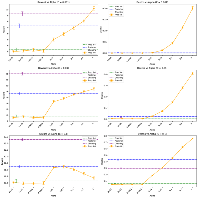
Results.
Figure 1 shows mean episode rewards and episode deaths under each guardrail across episodes, for different values of the rejection threshold . The cheating guardrail achieves zero deaths for sufficiently small , but for its death probability is moderately high.888Indeed, if every action taken had a harm probability of , the probability of death across an episode would be . The posterior predictive guardrail also achieves zero deaths for small , while for larger it dies slightly more often and achieves somewhat lower reward compared to the cheating guardrail. The behaviour of the Proposition 4.6 guardrail depends strongly on . When is close to , actions are very rarely rejected, leading to a high probability of an early death and precluding the opportunity to obtain much reward. At the other extreme, when is close to , the candidate theory set is larger and the guardrail is extremely conservative. It rejects almost all actions, resulting in low deaths and low reward. This is the case even for larger , since the estimated probability used to filter actions tends to overestimate an action’s harm probability under the true theory. For middling values of , the Proposition 4.6 guardrail performs similarly to the posterior predictive guardrail. The Proposition 3.4 guardrail, which makes the incorrect assumptions of i.i.d. data and distinct theories, is similarly conservative to the Proposition 4.6 guardrail with low .
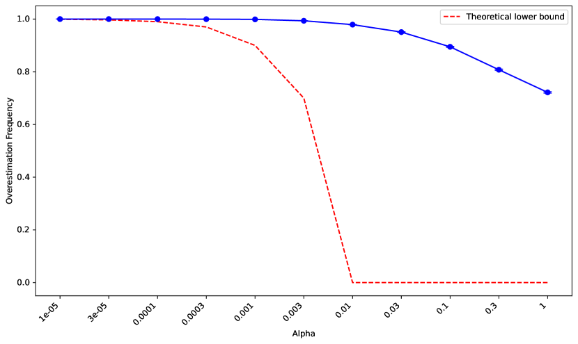
Tightness of bounds.
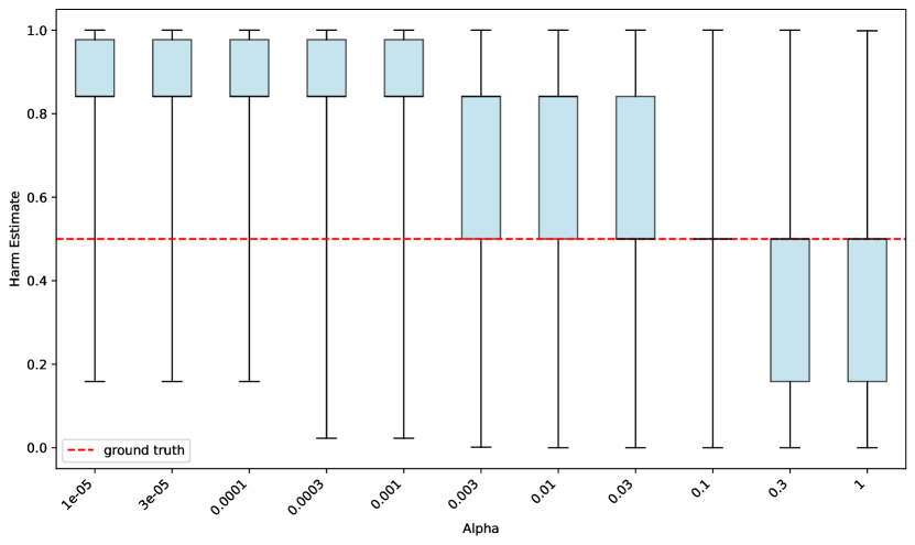
Figure 2 takes a closer look at how often, and how tightly, the inequality in Proposition 4.6 is satisfied. For an agent following a uniform policy across bandit episodes without action rejection or death, Figure 2(a) shows the frequency with which overestimates the true harm probability of an action. Proposition 4.6 gives us a strict lower bound of (which may be below ) on the overestimation frequency, but the frequency significantly exceeds the bound for large . Figure 2(b) shows the distribution of harm estimates for the most dangerous action, which always has a ground truth harm probability of due to the choice of . Note that for large the harm of this dangerous action is usually underestimated – so the high overestimation rate in Figure 2(a) comes from actions with lower harm probabilities.
6 Conclusion and open problems
The approach to safety verification proposed here is based on context-dependent run-time verification because the set of possible inputs for a machine learning system is generally astronomical, while the safety of the answer to a specific question is more likely to be amenable to tractable calculations. It focuses on the risk of wrongly interpreting the data, including the safety specification itself (what we called “harm” above) and exploits the fact that as more evidence is gathered (as necessarily happens with i.i.d. data) and when different theories predict different observations, the true interpretation rises towards the maximal value of the Bayesian posterior over interpretations. The bound is tighter with i.i.d. data but the i.i.d. assumption is also not realistic, and in the context of safety-critical decisions, we would prefer to err on the side of prudence and fewer assumptions. However, it provides an interesting template to think about variants of this idea in future work.
There are many open problems to consider before turning the kinds of bounds introduced above into an operational run-time safeguard:
-
1.
Upper-bounding overcautiousness. Can we ensure that we do not underestimate the probability of harm but do not massively overestimate it? Some simple theories consistent with the dataset (even an arbitrarily large one) might deem non-harmful actions harmful. Can we bound how much this harm-avoidance hampers the agent? A plausible approach would be to make use of a mentor for the agent that demonstrates non-harmful behavior [5].
-
2.
Tractability of posterior estimation. How can we efficiently estimate the required Bayesian posteriors? For computational tractability, a plausible answer would rely on amortized inference, which turns the difficult estimation of these posteriors into the task of training a neural net probabilistic estimator which will be fast at run-time. Recent work on amortized Bayesian inference for symbolic models, such as causal structures [9, 10], and for intractable posteriors in language models [16, 18, 36, 35, 39] – which are useful when prior knowledge is encoded in a pretrained foundation model – suggests that this is feasible. Advances in efficient and adaptive Monte Carlo methods, e.g., for language models [29, 42, 23], can also be useful for this purpose, and MCMC approaches can complement and aid amortization [17, 21, 31, 20].
-
3.
Efficient search for a cautious theory. How can we efficiently identify a cautious but plausible theory that upper-bounds the risk, since this requires an optimization at run-time? Again, a plausible answer is to rely on amortized probabilistic inference, e.g., by sampling theories with a low or annealed temperature, a technique that has been used for decades in the nonconvex optimization literature and more recently combined with amortized sequential sampling methods [40, 41, 43, inter alia].
-
4.
Partial specification of theories. Another issue is that a full explanatory theory for the evidence will generally be too large an object to make the above bound calculations and optimization sufficiently efficient. An alternative would be to derive bounds that only require partial explanations, similarly to how humans tell cautious ‘stories’ about what could go wrong in uncertain circumstances when thinking about taking a potentially dangerous decision [3].
-
5.
Harm specification in natural language. How is a safety specification provided in natural language, like with Constitutional AI [1], turned into a random variable over which conditional probabilities can be estimated? Having humans label lots of situations that match the desired constraint seems impractical. The alternative proposed by Bengio [3] is to learn to interpret natural language statements as formal random variables over which probabilistic causal reasoning can occur. The ambiguity of natural language can then be captured by having a distribution over formal interpretations.
-
6.
Effect of approximation error. Finally, because we envisage using machine learning to estimate the bound, we have to consider the fact that a learned predictor will be imperfect. How do we correct conservatively for the potentially dangerous errors made by this predictor? This may be particularly important if we use a neural network to estimate probabilities, since they are subject to lack of robustness and adversarial attacks [15, 38], e.g., how do we make sure that the agent proposing the actions has not learned to find loopholes in the risk estimator?
References
- Bai et al. [2022] Yuntao Bai, Saurav Kadavath, Sandipan Kundu, Amanda Askell, Jackson Kernion, Andy Jones, Anna Chen, Anna Goldie, Azalia Mirhoseini, Cameron McKinnon, et al. Constitutional AI: Harmlessness from AI feedback. arXiv preprint arXiv:2212.08073, 2022.
- Barron et al. [1999] Andrew Barron, Mark J. Schervish, and Larry Wasserman. The consistency of posterior distributions in nonparametric problems. The Annals of Statistics, 27(2):536–561, 1999.
- Bengio [2024] Yoshua Bengio. Towards a cautious scientist AI with convergent safety bounds, February 2024. URL https://yoshuabengio.org/2024/02/26/towards-a-cautious-scientist-ai-with-convergent-safety-bounds/.
- Bengio et al. [2024] Yoshua Bengio, Daniel Privitera, Tamay Besiroglu, Rishi Bommasani, Stephen Casper, Yejin Choi, Danielle Goldfarb, Hoda Heidari, Leila Khalatbari, Shayne Longpre, et al. International Scientific Report on the Safety of Advanced AI. PhD thesis, Department for Science, Innovation and Technology, 2024.
- Cohen and Hutter [2020] Michael K Cohen and Marcus Hutter. Pessimism about unknown unknowns inspires conservatism. Conference on Learning Theory (COLT), 2020.
- Cohen et al. [2022a] Michael K Cohen, Marcus Hutter, and Neel Nanda. Fully general online imitation learning. Journal of Machine Learning Research, 23(1):15066–15095, 2022a.
- Cohen et al. [2022b] Michael K. Cohen, Marcus Hutter, and Michael A. Osborne. Advanced artificial agents intervene in the provision of reward. AI magazine, 43(3):282–293, 2022b.
- Dalrymple et al. [2024] David Dalrymple, Joar Skalse, Yoshua Bengio, Stuart Russell, Max Tegmark, Sanjit Seshia, Steve Omohundro, Christian Szegedy, Ben Goldhaber, Nora Ammann, et al. Towards guaranteed safe AI: A framework for ensuring robust and reliable AI systems. arXiv preprint arXiv:2405.06624, 2024.
- Deleu et al. [2022] Tristan Deleu, António Góis, Chris Emezue, Mansi Rankawat, Simon Lacoste-Julien, Stefan Bauer, and Yoshua Bengio. Bayesian structure learning with generative flow networks. Uncertainty in Artificial Intelligence (UAI), 2022.
- Deleu et al. [2023] Tristan Deleu, Mizu Nishikawa-Toomey, Jithendaraa Subramanian, Nikolay Malkin, Laurent Charlin, and Yoshua Bengio. Joint Bayesian inference of graphical structure and parameters with a single generative flow network. Neural Information Processing Systems (NeurIPS), 2023.
- Diaconis and Freedman [1986] Persi Diaconis and David A. Freedman. On the consistency of Bayes estimates (with discussion). The Annals of Statistics, 14:1–26, 1986.
- Doob [1949] J.L. Doob. Application of the theory of martingales. Colloque International Centre Nat. Rech. Sci., pages 22–28, 1949.
- Freedman [1963] David A. Freedman. On the asymptotic behavior of Bayes’ estimates in the discrete case. The Annals of Mathematical Statistics, 34(4):1386–1403, 1963.
- Freedman [1965] David A. Freedman. On the asymptotic behavior of Bayes estimates in the discrete case II. The Annals of Mathematical Statistics, 36(2):454–456, 1965.
- Goodfellow et al. [2015] Ian J Goodfellow, Jonathon Shlens, and Christian Szegedy. Explaining and harnessing adversarial examples. International Conference on Learning Representations (ICLR), 2015.
- Guo et al. [2021] Han Guo, Bowen Tan, Zhengzhong Liu, Eric P. Xing, and Zhiting Hu. Efficient (soft) Q-learning for text generation with limited good data. arXiv preprint arXiv:2106.07704, 2021.
- Hu et al. [2023] Edward J. Hu, Nikolay Malkin, Moksh Jain, Katie Everett, Alexandros Graikos, and Yoshua Bengio. GFlowNet-EM for learning compositional latent variable models. International Conference on Machine Learning (ICML), 2023.
- Hu et al. [2024] Edward J. Hu, Moksh Jain, Eric Elmoznino, Younesse Kaddar, Guillaume Lajoie, Yoshua Bengio, and Nikolay Malkin. Amortizing intractable inference in large language models. International Conference on Learning Representations (ICLR), 2024.
- Karwowski et al. [2023] Jacek Karwowski, Oliver Hayman, Xingjian Bai, Klaus Kiendlhofer, Charlie Griffin, and Joar Skalse. Goodhart’s law in reinforcement learning. arXiv preprint arXiv:2310.09144, 2023.
- Kim et al. [2024a] Minsu Kim, Sanghyeok Choi, Jiwoo Son, Hyeonah Kim, Jinkyoo Park, and Yoshua Bengio. Ant colony sampling with GFlowNets for combinatorial optimization. arXiv preprint arXiv:2403.07041, 2024a.
- Kim et al. [2024b] Minsu Kim, Taeyoung Yun, Emmanuel Bengio, Dinghuai Zhang, Yoshua Bengio, Sungsoo Ahn, and Jinkyoo Park. Local search GFlowNets. International Conference on Learning Representations (ICLR), 2024b.
- Krakovna et al. [2020] Victoria Krakovna, Jonathan Uesato, Vladimir Mikulik, Matthew Rahtz, Tom Everitt, Ramana Kumar, Zac Kenton, Jan Leike, and Shane Legg. Specification gaming: the flip side of AI ingenuity, 2020. URL deepmind.com/blog/specification-gaming-the-flip-side-of-ai-ingenuity.
- Lew et al. [2023] Alexander K Lew, Tan Zhi-Xuan, Gabriel Grand, and Vikash K Mansinghka. Sequential Monte Carlo steering of large language models using probabilistic programs. arXiv preprint arXiv:2306.03081, 2023.
- McNeil et al. [2015] Alexander J McNeil, Rüdiger Frey, and Paul Embrechts. Quantitative risk management: concepts, techniques and tools-revised edition. Princeton university press, 2015.
- Miller [2018] Jeffrey W. Miller. A detailed treatment of Doob’s theorem. arXiv preprint arXiv:1801.03122, 2018.
- Miller [2021] Jeffrey W. Miller. Asymptotic normality, concentration, and coverage of generalized posteriors. Journal of Machine Learning Research, 22(168):1–53, 2021.
- Pan et al. [2021] Alexander Pan, Kush Bhatia, and Jacob Steinhardt. The Effects of Reward Misspecification: Mapping and Mitigating Misaligned Models. In International Conference on Learning Representations, 2021.
- Pang et al. [2023] Richard Yuanzhe Pang, Vishakh Padmakumar, Thibault Sellam, Ankur P. Parikh, and He He. Reward Gaming in Conditional Text Generation. arXiv preprint arXiv:2211.08714, 2023.
- Phan et al. [2023] Du Phan, Matthew D. Hoffman, David Dohan, Sholto Douglas, Tuan Anh Le, Aaron Parisi, Pavel Sountsov, Charles Sutton, Sharad Vikram, and Rif A. Saurous. Training chain-of-thought via latent-variable inference. Neural Information Processing Systems (NeurIPS), 2023.
- Schwartz [1965] Lorraine Schwartz. On Bayes procedures. Probability Theory and Related Fields, 4(1):10–26, 1965.
- Sendera et al. [2024] Marcin Sendera, Minsu Kim, Sarthak Mittal, Pablo Lemos, Luca Scimeca, Jarrid Rector-Brooks, Alexandre Adam, Yoshua Bengio, and Nikolay Malkin. Improved off-policy training of diffusion samplers. arXiv preprint arXiv:2402.05098, 2024.
- Skalse et al. [2024] Joar Skalse, Lucy Farnik, Sumeet Ramesh Motwani, Erik Jenner, Adam Gleave, and Alessandro Abate. STARC: A general framework for quantifying differences between reward functions. arXiv preprint arXiv:2309.15257, 2024.
- Skalse et al. [2022] Joar Max Viktor Skalse, Nikolaus H. R. Howe, Dmitrii Krasheninnikov, and David Krueger. Defining and characterizing reward gaming. Neural Information Processing Systems (NeurIPS), 2022.
- Skalse et al. [2023] Joar Max Viktor Skalse, Matthew Farrugia-Roberts, Stuart Russell, Alessandro Abate, and Adam Gleave. Invariance in policy optimisation and partial identifiability in reward learning. International Conference on Machine Learning (ICML), 2023.
- Song et al. [2024] Zitao Song, Chao Yang, Chaojie Wang, Bo An, and Shuang Li. Latent logic tree extraction for event sequence explanation from LLMs. International Conference on Machine Learning (ICML), 2024.
- Venkatraman et al. [2024] Siddarth Venkatraman, Moksh Jain, Luca Scimeca, Minsu Kim, Marcin Sendera, Mohsin Hasan, Luke Rowe, Sarthak Mittal, Pablo Lemos, Emmanuel Bengio, Alexandre Adam, Jarrid Rector-Brooks, Yoshua Bengio, Glen Berseth, and Nikolay Malkin. Amortizing intractable inference in diffusion models for vision, language, and control. arXiv preprint arXiv:2405.20971, 2024.
- Ville [1939] Jean Ville. Étude critique de la notion de collectif. 1939. URL http://eudml.org/doc/192893.
- Wei et al. [2023] Alexander Wei, Nika Haghtalab, and Jacob Steinhardt. Jailbroken: How does LLM safety training fail? Neural Information Processing Systems (NeurIPS), 2023.
- Yu et al. [2024] Fangxu Yu, Lai Jiang, Haoqiang Kang, Shibo Hao, and Lianhui Qin. Flow of reasoning: Efficient training of LLM policy with divergent thinking. arXiv preprint arXiv:2406.05673, 2024.
- Zhang et al. [2023a] David Zhang, Corrado Rainone, Markus Peschl, and Roberto Bondesan. Robust scheduling with GFlowNets. International Conference on Learning Representations (ICLR), 2023a.
- Zhang et al. [2023b] Dinghuai Zhang, Hanjun Dai, Nikolay Malkin, Aaron Courville, Yoshua Bengio, and Ling Pan. Let the flows tell: Solving graph combinatorial problems with GFlowNets. Neural Information Processing Systems (NeurIPS), 2023b.
- Zhao et al. [2024] Stephen Zhao, Rob Brekelmans, Alireza Makhzani, and Roger Baker Grosse. Probabilistic inference in language models via twisted sequential Monte Carlo. International Conference on Machine Learning (ICML), 2024.
- Zhou et al. [2024] Ming Yang Zhou, Zichao Yan, Elliot Layne, Nikolay Malkin, Dinghuai Zhang, Moksh Jain, Mathieu Blanchette, and Yoshua Bengio. PhyloGFN: Phylogenetic inference with generative flow networks. International Conference on Learning Representations (ICLR), 2024.
- Zhuang and Hadfield-Menell [2020] Simon Zhuang and Dylan Hadfield-Menell. Consequences of misaligned AI. Neural Information Processing Systems (NeurIPS), 2020.