Strategic Allocation of Battery Electric Bus Chargers under Stochastic Demand: A Chicago Case Study using Metaheuristic Approaches

Abstract

Bus electrification accelerates the transition towards sustainable urban transportation. Battery-Electric Buses (BEBs) often require periodic recharging intervals between service trips. The strategic placement and allocation of charging equipment are crucial in facilitating operations, optimizing costs, and minimizing downtime. In this study, we develop an optimization framework to address the optimal placement of various charger types at candidate locations under the stochastic charging demand of BEBs. The framework aims to minimize long-term system costs while balancing considerations among station, charger, and value of time expenses. Leveraging existing stochastic location literature, we develop a mixed-integer non-linear program (MINLP) to model the problem. We design an exact solution method to address this computationally challenging problem. The program optimizes the generalized costs associated with building charging stations, allocating charger types, traveling to charging stations, and average queueing and charging times. Queueing dynamics are modeled using an M/M/s queue, with the number of servers as a decision variable at each candidate location and each charger type. The linearization process, which excludes queueing variables, is succeeded by introducing associated constraints through cutting planes. This step guarantees global optimality due to the convexity properties of the problem. To enhance scalability, we implement a genetic algorithm and a simulated annealing metaheuristic and devise heuristic clustering strategies, facilitating the effective resolution of real-world, large-scale instances. Then, we conduct comparative analyses across garage-only, other-only, and mixed-location scenarios.

Keywords: Battery Electric Buses, Charging Scheduling, Stochastic Charger Location and Allocation, Optimization, Simulated Annealing, Genetic Algorithm

1 Introduction

With more than two-thirds of the world’s population predicted to live in cities by 2050 [1], urban transportation networks will play a vital role in enhancing the quality of life and the functionality of cities by providing essential mobility and accessibility to residents. Public transportation, in particular, is key to reducing traffic congestion, lowering emissions, and providing equitable access to transportation. However, transportation substantially contributes to air pollution, with the transportation sector being one of the largest producers of carbon dioxide [2, 3]. Reducing these emissions is critical in the fight against climate change, and one promising solution is the adoption of vehicles powered by alternative fuels, such as electric, hybrid, and hydrogen-powered vehicles [4, 5].

One significant step towards reducing carbon emissions and noise pollution in urban areas is the electrification of public transportation bus fleets [2, 6]. Numerous cities worldwide are transitioning to battery-electric buses (BEBs) to achieve this goal [2, 5, 7]. For instance, the Chicago Transit Authority (CTA) has committed to transitioning to a fully electric bus fleet by 2040 [8]. The benefits of BEBs include zero tailpipe emissions, reduced maintenance costs due to fewer moving parts, decreased noise pollution, reduced vibration, enhanced passenger comfort, and lower fuel and maintenance costs [7, 2, 3, 5]. However, BEBs also come with challenges such as limited travel range, long charging times, increased planning complexity, and high initial costs for both the buses and the required charging infrastructure [9, 6, 2, 5].

There are two prevailing approaches to charging BEBs: on-route charging at terminal points —including a bus garage and other locations— using fast chargers and overnight charging with slow chargers at the garage. On-route charging is faster but requires more chargers and infrastructure [7], while slow chargers are cheaper but necessitates a larger fleet to cover all scheduled trips and put significant demand on the power grid at night [10]. A balanced approach is essential, as relying solely on garage charging would require a larger fleet and cause grid strain, while exclusive reliance on on-route charging would lead to increased costs due to the need for more chargers and stations.

The problem of optimizing the location of charging stations and the allocation of chargers involves balancing the costs of building stations and allocating chargers with the operational costs associated with bus waiting times and travel times for charging. Increasing the number of stations can reduce the travel costs, as buses can quickly reach nearby stations when they need to charge. Similarly, increasing the number of chargers at each station potentially reduces waiting times, as buses spend less time queuing to charge. On the other hand, adding the possible redundancy comes at a high deployment cost. To this end, a balanced objective approach [11] will equilibrate the level of deployment and the cost of potential queueing and travel.

To address this problem, we develop an optimization framework that jointly finds the optimal locations for charging stations and the number of fast and slow chargers at each candidate station. The framework is composed of two steps, and LABEL:procedure depicts a flowchart of the framework. In the first step, we solve the Single Depot Vehicle Scheduling Problem (SDVSP) for buses assuming they are not constrained by an electric driving range. In the SDVSP, revenue-generating timetabled trips are chained into bus schedule blocks while minimizing the total intertrip layover time, deadheading time, and the number of blocks. In this step, we identify potential locations where recharging demand emerge by segmenting blocks based on a BEB range and mapping the corresponding trip terminals. In the second step, we extend a model belonging to the Stochastic Location Models with Congestion, Immobile Server, and Balanced Objective (SLCIS-BO) literature to find the optimal location, number, and type of chargers [11]. The problem is hence modeled with a Mixed-Integer Non-Linear Program (MINLP). The stochastic nature of the problem is addressed utilizing the queuing theory, and the impact of average waiting times at chargers is incorporated into the location and allocation decision-making. Since the problem scale dealt with is large, this step also involves a post-processing of the solutions obtained through the first step to control the problem size. In the post-processing, recharging demand locations are clustered to control the problem size. The main foccus of this paper is the SLCIS-BO modeling and the three solution methods presented: exact solution, Genetic Algorithm (GA), and Simulated Annealing (SA) algorithm. The first step prepares the input data for this model, and the clustering approach controls the problem size to achieve good quality solutions with the exact solution method under reasonable computational restraints.

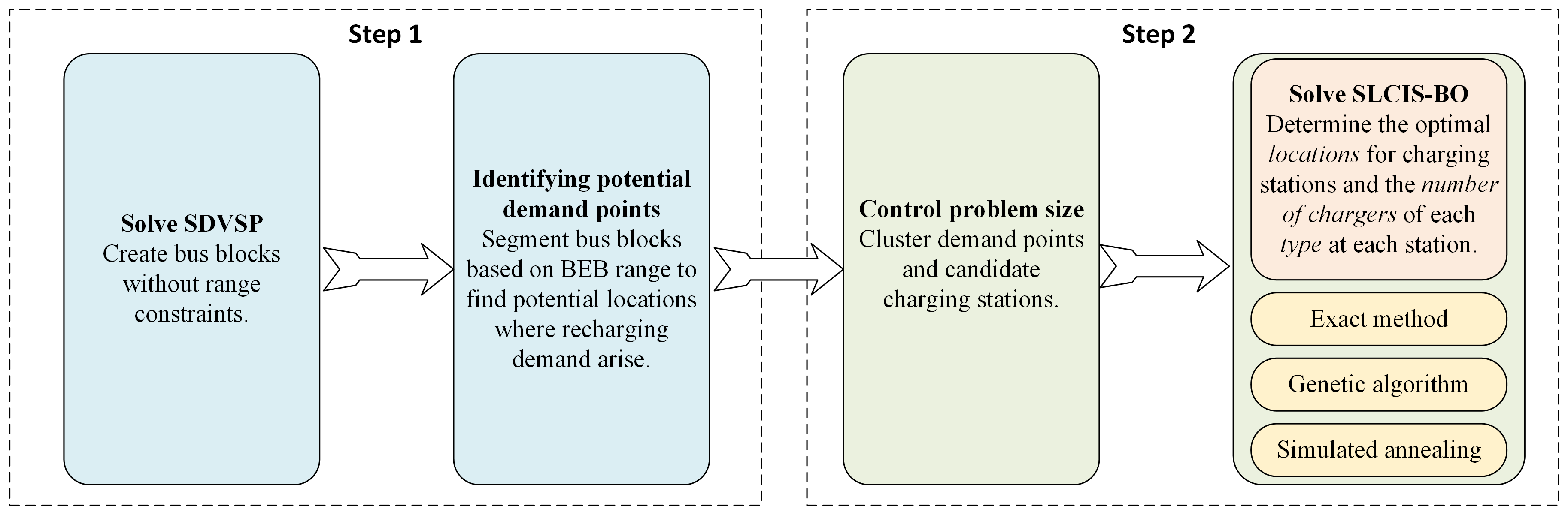
Figure 1: Procedure of the Study

fig]procedure

The exact solution algorithm is derived through adopting cutting-plane constraints. While the algorithm finds optimal solutions to small-scale problems quickly, large-scale problems require unfavorably large computational times. Therefore, we propose two metaheuristic approaches: a GA and an SA algorithm. In our case studies, we focus on Chicago’s public transportation system, specifically Chicago Transit Authority (CTA) and PACE Suburban Bus.

Contributions of the paper are outlined as follows:

• The recharging demand stochasticity is integrated into charger location and allocation decisions. The stochasticity aspect was considered only in a few studies, and this study extends upon the SLCIS-BO literature with an application into the BEB context.

• The literature does not consider a joint optimization of charger location and the number of different charger types in the urban transit electrification context. While integrating both, this study also takes the waiting time into account and fills the gap in the literature.

• Coverage constraints of the classical SLCIS-BO are replaced with subset representations to improve the robustness, and variable charger types are incorporated into the model.

• Meta-heuristic solution approaches are designed to address the scalability concern.

• Case studies are conducted using real-world bus networks in the Chicago, IL metropolitan region: Chicago Transit Authority (CTA) and PACE Suburban Bus.

2 Literature Review

With advancements in Electric Vehicle (EV) technologies and growing concerns about greenhouse gas emissions and the sustainability of transportation networks, many individuals and transportation companies are transitioning from internal combustion engine vehicles to EVs [7, 4]. Numerous studies have explored the deployment of charging infrastructure for both private and heavy-duty EVs. The urban transit sector offers significant potential for EV deployment, as buses typically operate on shorter trip distances and fixed routes, making them well-suited to the current limitations of battery range [4]. While many studies have focused on optimizing charging infrastructure for EVs in general [12, 13, 14], the unique characteristics of BEBs require special attention [7]. This has lead to several studies specifically targeting the placement of BEB charging stations in urban areas, aiming to provide efficient and cost-effective charging solutions while improving service levels for passengers [2, 15, 16, 4, 7, 5, 9, 17].

He et al. [14] tackled the problem of locating charging stations for EVs through a bi-level modeling approach. Their study addressed the relationship between charging station deployment and route selection. Their findings emphasized that the battery range of EVs and the distances driven significantly influence the optimal placement of charging infrastructure.

Rogge et al. [15] developed a model that simultaneously optimizes bus fleet size, vehicle scheduling, charger numbers, and charging schedules for transit systems employing BEBs. They employed a GA to solve this model and applied it in a case study involving 200 trips across 3 bus routes. The study’s limitation to garage charging assumed that BEBs return to the garage for recharging, and restricted its applicability to scenarios with on-route layover charging.

Wei et al. [16] introduced a spatio-temporal optimization model aimed at minimizing costs related to vehicle procurement and charging station allocation, while adhering to existing bus routes and schedules. Their MILP model identified optimal route assignments, as well as the locations and sizes of on-route layover charging stations and overnight charging sites at garages. They applied this model to the transit network operated by the Utah Transit Authority. However, their assumption that buses can fully charge during any layover period of 10 minutes or more makes their model impractical unless buses have small batteries or use extremely high-power chargers.

An [17] developed a stochastic integer model to solve the problem of optimizing the placement of plug-in chargers and fleet size for BEBs. The study considered time-varying electricity prices and the fluctuations in charge demand due to weather or traffic conditions. The model assumed vehicles may charge only between trips while maintaining the existing diesel bus operation schedule, aggregating demand at terminals based on battery levels. It established discrete one-hour charging time blocks, ensuring the total number of available blocks is not exceeded.

Hsu et al. [4] solved the problem of locating charging facilities for electrifying urban bus services, highlighting the transition from diesel to electric buses. Their optimization model addressed practical concerns such as fleet size, land acquisition, bus allocation, and deadhead mileage. They proposed a decomposition-based heuristic algorithm for computational efficiency and applied it to a bus operator in Taiwan.

Tzamakos et al. [2] developed a model for optimally locating fast wireless chargers in electric bus networks, accounting for bus delays due to queuing at charging locations. The integer linear programming model minimized investment costs for opportunity charging facilities, employing an M/M/1 queuing model to incorporate queuing delays. The results indicate the importance of considering waiting times when defining the number of charger stations. However, they only consider opportunity charging during bus service trips and do not include charging during layover times at garages or terminal stations.

He et al. [9] addressed the combined challenges of charging infrastructure planning, vehicle scheduling, and charging management for BEBs. Their MINLP formulation aimed to minimize the total cost of ownership, employing a genetic algorithm-based approach for solution. The study, applied to a sub-transit network in Salt Lake City, Utah, compared alternative scenarios to the optimal results, demonstrating the model’s effectiveness in developing cost-efficient planning strategies.

McCabe and Ban [5] presented the BEB optimal charger location model, an MILP approach to optimize the locations and sizes of layover charging stations for BEBs. The model balances infrastructure costs with operational performance, ensuring no bus waits at a charging location. Additionally, the BEB block revision problem model revises vehicle schedules to dispatch backup buses for trips at risk of running out of battery. They apply the model to a case study of King County, WA, and highlight the unique operational characteristics of bus systems and the benefits of strategic charger location decisions.

The reviewed studies collectively highlight the complexity and importance of strategic planning for charging infrastructure. Key considerations include minimizing costs, ensuring operational efficiency, and accommodating practical constraints such as waiting times, and driving ranges. The models and methodologies developed in these studies provide valuable insights and tools for transit agencies and planners aiming to optimize the deployment of BEB charging stations. LABEL:lit_sum compares this paper with relevant studies in the literature. The table highlights a significant gap: no existing methods optimize both the location of charging stations and the number of different types of chargers at each station while accounting for waiting times in an urban transit network. This paper aims to address this gap by developing an optimization model for the strategic placement of charging stations. Furthermore, the proposed meta-heuristic approaches ensure that the model can be effectively applied to real-world networks.

Table 1: A summary of the reviewed literature

tab]lit_sum

Reference	Location	Allocation	Urban Transit	Charger Types	Waiting Time	Charging Type	Model	Case Study
He et al. [14]	✓	✗	✗	✗	✗	terminals	bi-level	✗
Rogge et al. [15]	✓	✓	✓	✗	✗	garages	MILP	Aachen & Roskilde
Wei et al. [16]	✓	✓	✓	✗	✗	terminals & garages	MIP	Utah
An [17]	✓	✗	✓	✗	✗	terminals	stochastic integer program	Melbourne
Uslu and Kaya [3]	✓	✓	✗	✗	✓	terminals	MILP	Turkey
Hsu et al. [4]	✓	✗	✓	✗	✗	garages	augmented ILP	Taoyuan
Hu et al. [7]	✓	✗	✓	✗	✓	terminals	MILP	Sydney
Tzamakos et al. [2]	✓	✓	✓	✓	✓	terminals	ILP	✗
He et al. [9]	✗	✗	✓	✓	✗	terminals & garages	MINLP	Salt Lake City
McCabe and Ban [5]	✓	✓	✓	✗	✓	terminals & garages	MILP	King County Metro
This paper	✓	✓	✓	✓	✓	terminals & garages	MINLP	Chicago

Note: ILP: Integer Liner Programming, MILP: Mixed-Integer Linear Programming, MIP: Mixed Integer Programming

3 Methodology

In this section, we first provide a detailed explanation of the problem, followed by an outline of our assumptions. Next, we introduce the notations used in the model. Finally, we present the optimization model, explaining the objective function and all associated constraints.

3.1 Problem overview

The classical SDVSP involves creating bus blocks with a given set of timetabled service trips. Each trip represents a service plan with essential spatio-temporal information that are origin, destination, start time, and end time. The origin and destination are also called terminal points. The charger location problem is ideally solved in conjunction with the scheduling problem. However, the electrification occurs over time, that is transit agencies alter their fleets with the electric ones gradually. To this end, a typical BEB deployment behavior is to electrify existing routes and bus schedules rather than re-planning the entire system. To mimic this behavior, we begin with solving SDVSPs for each garage of a given transit agency using their trip information. Hence, the SDVSP solutions yield fossil fuel powered bus blocks. Blocks represent a sequence of consecutive trips between two garage visits [18]. Using these blocks and a given BEB range, we then partition blocks and find potential demand points from where BEBs could head to charging stations.

LABEL:blocksegmenting illustrates an example bus block including layover at the garage, deadheading from/to garage and trips, trip timing, layover time between trips, timing of recharge demand, and battery depletion time. Here, the bus starts the service at 6 AM, deadheads to another trip’s origin, serves the second trip, deadheads to the third trip’s origin, lays over at this terminal for an hour, and serves its third trip. We assume buses do not consume energy during layover. If this block is run by a BEB and assuming a BEB range of six hours, it can’t finish the fourth trip. The red vertical lines in the figure show the battery depletion time based on the BEB range and are called dividers. Buses are assumed to charge only when not in service, that is before or after a service trip similar to layover charging presented in [5]. Thus, although the battery depletes at 5 PM, the charging event will occur at 4 PM at the destination terminal of the third trip, which is the closest terminal stop before the battery depletion time. Assuming the bus fully recharges, the next charging demand arises at around 12 AM. Conducting a similar logic-based strategy for all bus blocks, we find demand points and the number of charging need at each point.

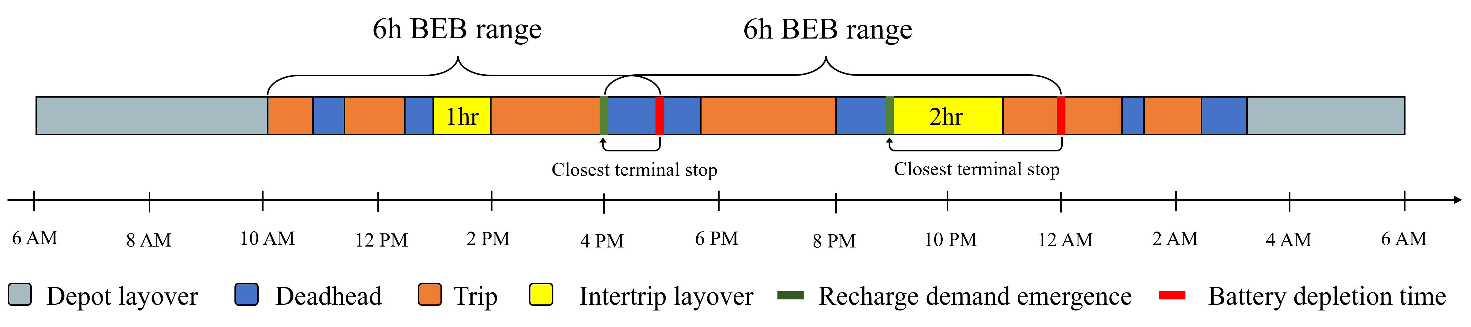
Figure 2: Identifying potential demand points

fig]blocksegmenting

LABEL:DemandFlowChart depicts the flowchart for positioning the dividers between trips of a BEB. It is worthwhile to note that the overall process in this figure is only one way to estimate potential demand points, and a different method for this estimation could be used.

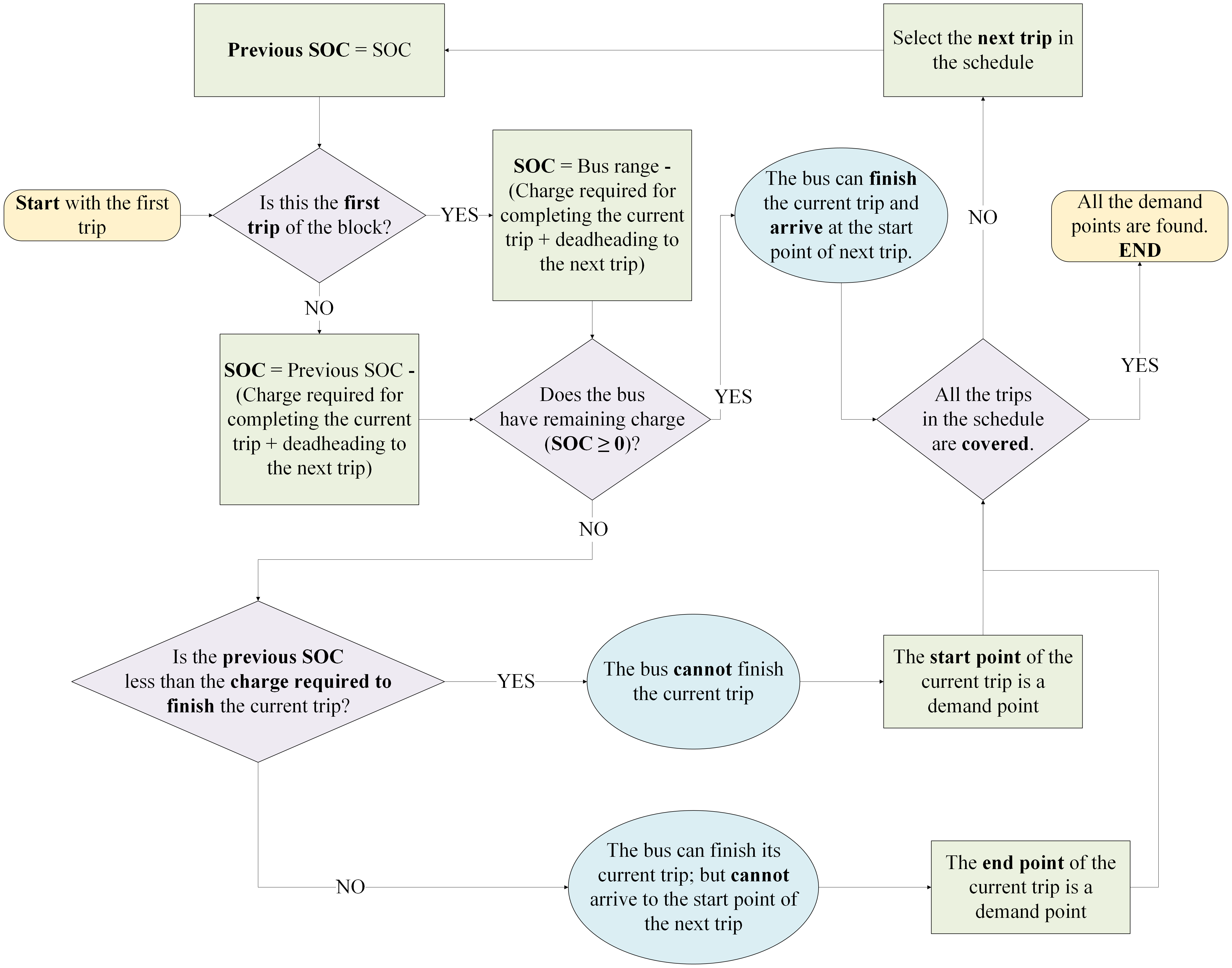
Figure 3: Flowchart for finding the demand points

fig]DemandFlowChart

All terminal stations and garages are considered to represent a set of candidate charging stations. The goal and the main focus of this study is to determine which stations to deploy a number of chargers with various types.

3.2 Assumptions

We formulate the model based on the following assumptions:

• The bus schedule and blocks are provided in advance [5, 7], which includes detailed information, such as trip start and end times, deadhead and layover times, terminal stops, and garages [5, 4, 2].

• All BEBs start their blocks with fully charged batteries [6, 5, 3].

• BEBs are homogeneous, including battery capacity, range, and efficiency [2, 4].

• Batteries operate within the range of 20% to 80% of their capacity [2].

• Energy consumption and gain are linearly correlated with time [5, 2].

• BEBs consume energy only when they are in service or deadheading to the next trip and do not consume any energy during layovers.

• The energy required for each trip and deadhead is a given parameter based on the duration of the trip [4, 2].

• Trips do not require more energy than the operational battery capacity [4].

• Charging stations can be equipped with both fast chargers and slow chargers, and each station may have multiple plugs of each type [2].

• The cost of constructing a charging station at garages is zero.

3.3 Mathematical model

Let $i\in\mathcal{I}$ denote a set of demand points from where BEBs head to chargers. Candidate charging stations are denoted by $j\in\mathcal{J}$, and the objective is to select a subset of them for charger deployment. The binary variable $y_{j}=1$ indicates that station $j$ is selected and incurs $C^{\phi}_{j}$ cost per time unit. A station from the subset $\mathcal{J}_{i}\subseteq\mathcal{J}$ can be visited to charge buses. This subset replaces the commonly adopted coverage constraints Berman and Krass [11, Ch. 17, pp. 486] such that additional constraints are not needed in the model to restrict the stations that could be visited. Considering all stations as potential locations to visit for charging both explodes the problem size and is unrealistic. The State-of-Charge (SOC) may not allow visiting any given station in the network. This subset could be refined based on a maximum travel distance/time from demand points to charging stations. We also define $\mathcal{I}_{j}$ as the subset of demand points from where BEBs can head to charging at station $j\in\mathcal{J}$. LABEL:notations lists all sets, parameters, and variables used in our mathematical model. Unless otherwise noted, all parameters are non-negative real numbers ($\mathbb{R}_{\geq 0}$).

Table 2: Sets, Parameters, and Variables Used in the Model.

tab]notations

Set	Definition
$\mathcal{I}$	set of charging demand occurrence points
$\mathcal{I}_{j}$	subset of charging demand occurrence points from where BEBs can head to charging station $j\in\mathcal{J}$
$\mathcal{J}$	set of candidate charging stations
$\mathcal{J}_{i}$	subset of charging stations that could be visited from charging demand occurrence point $i\in\mathcal{I}$
$\mathcal{K}$	set of charger types
Variable	Definition
$s_{jk}$	number of type $k$ chargers allocated to station $j\in\mathcal{J}$, $s_{jk}\in\mathbb{Z}_{\geq 0}$
$W_{jk}$	expected waiting time for charger $k\in\mathcal{K}$ at station $j\in\mathcal{J}$, $W_{jk}\in\mathbb{R}_{\geq 0}$
$x_{ijk}$	$1$ if charger type $k\in\mathcal{K}$ at station $j\in\mathcal{J}_{i}$ is visited before $i\in\mathcal{I}$, $0$ otherwise
$y_{j}$	$1$ if station $j\in\mathcal{J}$ is active, $0$ otherwise
Parameter	Definition
$\epsilon$	an infinitesimal number
$\lambda_{i}$	charging demand rate for point $i\in\mathcal{I}$
$\mu_{k}$	service rate of charger type $k\in\mathcal{K}$
$C^{\delta}$	cost of travel time per time unit
$C^{\phi}_{j}$	fixed cost of charging station $j\in\mathcal{J}$ per time unit
$C^{\xi}_{k}$	cost of installing a type $k$ charger per time unit
$T_{ij}^{\delta}$	travel time from $i\in\mathcal{I}$ to $j\in\mathcal{J}$

There are a set of $\mathcal{K}$ charger types with various power output to be allocated to stations. The service rate for chargers, i.e., the number of vehicles that can be charged per time unit, is denoted by $\mu_{k}$ and depends on the initial SOC of vehicles before charging. Yet, the SOC is not tracked in the stochastic environment, and hence every BEB recharging at stations are assumed to recharge to their maximum battery capacity and the recharging time is fixed regardless of the initial SOC. Let binary variable $x_{ijk}=1$ denote that charger type $k\in\mathcal{K}$ at station $j\in\mathcal{J}_{i}$ is visited to charge a BEB traveling from demand point $i\in\mathcal{I}$. The number of type $k$ chargers, each incurring $C^{\xi}_{k}$ cost per time unit, allocated to station $j$ is denoted by variable $s_{jk}\in\mathbb{Z}_{\geq 0}$.

Travel time from $i\in\mathcal{I}$ to $j\in\mathcal{J}$ is denoted by $T_{ij}^{\delta}$. The travel time between demand points and charging stations incurs a cost of $C^{\delta}$ per time unit and is penalized in the objective function to encourage close proximity assignments.

The expected queue for each type $k$ at $j$ is modeled with an $M$/$M$/$s_{jk}$ queue, where charging demand and supply rates are assumed to follow a Poisson process. In this model, BEBs to be recharged by type $k$ at $j$ form into a single queue, and the service is provided with a first come, first served basis. Out of the $M$/$M$/$s_{jk}$ queue performance metrics, we are particularly interested in the expected wait time $\mathbb{W}(\sum_{i\in\mathcal{I}_{j}}\lambda_{i}x_{ijk},\mu_{k},s_{jk})$ inclusive of queueing and charging at charger type $k$ of station $j$, and the metric is a function of demand rate serviced by the station, $\mu_{k}$, and $s_{jk}$. Charger utilization rate $\rho_{jk}=\sum_{i\in\mathcal{I}_{j}}\lambda_{i}x_{ijk}/(\mu_{k}s_{jk})$. The condition $\rho_{jk}<1$ needs to be satisfied for queue stability, and we transform this into the linear constraint form $\mu_{k}s_{jk}(1-\epsilon)\geq\sum_{i\in\mathcal{I}_{j}}\lambda_{i}x_{ijk}~{}\forall j\in\mathcal{J},k\in\mathcal{K}$. The probability that all $s_{jk}$ chargers are busy is denoted by $\mathbb{P}(\sum_{i\in\mathcal{I}_{j}}\lambda_{i}x_{ijk},\mu_{k},s_{jk})$ and feeds into $\mathbb{W}(\cdot)$. Closed form formulations for both terms provided below can be found in the queueing theory literature. Equations 1 and 2 adapted into our notation conventions are from Winston [19]. We assume $\mathbb{P}(\cdot)=0$ when $s_{jk}=0$. The expected wait time to receive charging service with charger type $k$ at station $j$ is denoted by variable $W_{jk}\in\mathbb{R}_{\geq 0}$, and its associated probabilistic queue waiting time and charging service time cost is $C^{\tau}$ per time unit.

$$\mathbb{P}\left(\sum_{i\in\mathcal{I}_{j}}\lambda_{i}x_{ijk},\mu_{k},s_{jk}\right)=\frac{(\rho_{jk}s_{jk})^{s_{jk}}}{(1-\rho_{jk})s_{jk}!}\bigg{(}\frac{(\rho_{jk}s_{jk})^{s_{jk}}}{(1-\rho_{jk})s_{jk}!}+\sum_{r=0}^{s_{jk}-1}\frac{(\rho_{jk}s_{jk})^{r}}{r!}\bigg{)}^{-1}$$ (1)

$$\mathbb{W}\left(\sum_{i\in\mathcal{I}_{j}}\lambda_{i}x_{ijk},\mu_{k},s_{jk}\right)=\frac{\mathbb{P}(\sum_{i\in\mathcal{I}_{j}}\lambda_{i}x_{ijk},\mu_{k},s_{jk})}{\mu_{k}s_{jk}(1-\rho_{jk})}+\frac{1}{\mu_{k}}$$ (2)

We formulate a general MINLP model called model $\mathbb{G}$. It was introduced as a classical approach to model the SLCIS-BO in [11]. Our contribution in this general form is the inclusion of charger type $k$ and the reduction of coverage constraints using subset $\mathcal{J}_{i}$.

$$\min\mathbb{C}=\sum_{j\in\mathcal{J}}C^{\phi}_{j}y_{j}+\sum_{j\in\mathcal{J},k\in\mathcal{K}}C^{\xi}_{k}s_{jk}+\sum_{i\in\mathcal{I},j\in\mathcal{J}_{i},k\in\mathcal{K}}\lambda_{i}(C^{\delta}T^{\delta}_{ij}+C^{\tau}W_{jk})x_{ijk}$$ (3)

subject to,

$$x_{ijk}\leq y_{j}\qquad\forall i\in\mathcal{I}_{j},j\in\mathcal{J},k\in\mathcal{K}$$ (4)

$$\sum_{j\in\mathcal{J}_{i},k\in\mathcal{K}}x_{ijk}=1\qquad\forall i\in\mathcal{I}$$ (5)

$$\sum_{j^{\prime}\in\mathcal{J}_{i},k\in\mathcal{K}}T^{\delta}_{ij^{\prime}}x_{ij^{\prime}k}\leq(T^{\delta}_{ij}-\mathbb{M})y_{j}+\mathbb{M}\qquad\forall i\in\mathcal{I}_{j},j\in\mathcal{J}$$ (6)

$$\mu_{k}s_{jk}(1-\epsilon)\geq\sum_{i\in\mathcal{I}_{j}}\lambda_{i}x_{ijk}\qquad\forall j\in\mathcal{J},k\in\mathcal{K}$$ (7)

$$W_{jk}\geq\mathbb{W}(\sum_{i\in\mathcal{I}_{j}}\lambda_{i}x_{ijk},\mu_{k},s_{jk})\qquad\forall j\in\mathcal{J},k\in\mathcal{K}$$ (8)

$$x_{ijk},~{}y_{j}\in\{0,1\}\qquad\forall i\in\mathcal{I}_{j},j\in\mathcal{J},k\in\mathcal{K}$$ (9)

$$W_{jk}\in\mathbb{R}_{\geq 0},~{}s_{jk}\in\mathbb{Z}_{\geq 0}\qquad\forall j\in\mathcal{J},k\in\mathcal{K}$$ (10)

Objective function 3 minimizes the total station, charger, travel, and waiting (inclusive of charging time) costs per time unit denoted by $\mathbb{C}$. Constraints 4 ensure that demand point $i\in\mathcal{I}$ can use charger type $k\in\mathcal{K}$ at station $j\in\mathcal{J}$ only if station $j$ is active. Constraints 5, called single sourcing constraints by Berman and Krass [11], enforce that each demand point $i\in\mathcal{I}$ uses exactly one charger type $k\in\mathcal{K}$ at one station $j\in\mathcal{J}$. Constraints 6 ensure that a demand point is assigned to the closest selected station.

Constraints 7 and 8 are related to queueing theory and set an upper bound for utilization rate and a lower bound for service inclusive waiting time, respectively. Constraints 7 satisfy the queue stability condition $\rho_{jk}<1$, that is the service rate per charger type is strictly greater than the charging demand rate. Note that constraints 8 can be written in equality. Constraints 9 and 10 define the variable domains.

4 Solution approaches

4.1 An exact solution method

Grassmann [20] proved that $\sum_{i\in\mathcal{I}_{j}}\lambda_{i}x_{ijk}\mathbb{W}(\cdot)$ is convex in $\rho_{jk}$. Lee and Cohen [21] proved the Erlang delay formula to be strictly increasing and convex in $\rho_{jk}$, and noted that $\mathbb{W}(\cdot)$ satisfies the same condition as in 1. This property is used to derive an exact solution method that relies on the cutting-plane method.

Property 1.

$\mathbb{W}(\cdot)$ is strictly increasing and convex in $0<\rho_{jk}<1$.

The model is nonlinear due to $W_{jk}$. Let $q_{ijk}\in\mathbb{R}_{\geq 0}$ denote the travel and charging time inclusive waiting costs per time unit, which is the last component of the objective function 3. Let $\overline{S}_{jk}$ be the maximum number of chargers of type $k$ that can be allocated to $j$, and let $\mathcal{S}=\{0,1,2,\ldots,\max_{j\in\mathcal{J},k\in\mathcal{K}}\overline{S}_{jk}\}$ denote a set of all possible discrete number of chargers to be allocated. The number of chargers given $c\in\mathcal{S}$ is then denoted by the parameter $S_{c}$. We introduce the binary variable $z_{cjk}=1~{}\forall c\in\mathcal{S},~{}j\in\mathcal{J},~{}k\in\mathcal{K}$ to indicate if $c$ number of type $k$ chargers are allocated to $j$. We now need to restrain $z_{cjk}=1$ for only one $c\in\mathcal{S}$ given $j$ and $k$. Finally, we replace 3 with 11 and introduce 12–16. After these definitions and replacements, $W_{jk}$ and therefore constraints 8 and 12 remain non-linear, which are addressed next.

$$\min\mathbb{C}=\sum_{j\in\mathcal{J}}C^{\phi}_{j}y_{j}+\sum_{j\in\mathcal{J},k\in\mathcal{K}}C^{\xi}_{k}s_{jk}+\sum_{i\in\mathcal{I},j\in\mathcal{J}_{i},k\in\mathcal{K}}q_{ijk}$$ (11)

$$q_{ijk}\geq\lambda_{i}(C^{\delta}T^{\delta}_{ij}+C^{\tau}W_{jk})-\mathbb{M}(1-x_{ijk})\qquad\forall i\in\mathcal{I},j\in\mathcal{J}_{i},k\in\mathcal{K}$$ (12)

$$s_{jk}=\sum_{c\in\mathcal{S}}S_{c}z_{cjk}\qquad\forall j\in\mathcal{J},k\in\mathcal{K}$$ (13)

$$\sum_{c\in\mathcal{S}}z_{cjk}=1\qquad\forall j\in\mathcal{J},k\in\mathcal{K}$$ (14)

$$q_{ijk}\in\mathbb{R}_{\geq 0}\qquad\forall i\in\mathcal{I}_{j},j\in\mathcal{J},k\in\mathcal{K}$$ (15)

$$z_{cjk}\in\{0,1\}\qquad\forall c\in\mathcal{S},j\in\mathcal{J},k\in\mathcal{K}$$ (16)

Following 1 and the cutting-plane method proposed in [22], we will iteratively enforce lower bounds to $\mathbb{W}(\cdot)$. Let $\mathbb{W}^{\nu}(\rho_{jk})$ defined in 17 represent a portion of $\mathbb{W}(\cdot)$, and notice that 1 applies to $\mathbb{W}^{\nu}(\rho_{jk})$ as well.

$$\mathbb{W}^{\nu}(\rho_{jk})=\frac{\mathbb{P}(\sum_{i\in\mathcal{I}_{j}}\lambda_{i}x_{ijk},\mu_{k},s_{jk})}{1-\rho_{jk}}$$ (17)

Let $\tilde{\rho}_{jk}$ represent an approximation to $\rho_{jk}$, $B_{jk}=\partial\mathbb{W}^{\nu}(\tilde{\rho}_{jk})/\partial\tilde{\rho}_{jk}$, and $A_{jk}=\mathbb{W}^{\nu}(\tilde{\rho}_{jk})-B_{jk}\tilde{\rho}_{jk}$. Then, the linear line $A_{jk}+B_{jk}\rho_{jk}$ supports $\mathbb{W}^{\nu}(\cdot)$ at $\rho_{jk}=\tilde{\rho}_{jk}$, and we write $W_{jk}\geq(A_{jk}+B_{jk}\rho_{jk})/(\mu_{k}S_{c})+1/\mu_{k}$. Introducing this constraint conditional upon values of $S_{c}$, $A_{jk}$, $B_{jk}$, $x_{ijk}$, and $z_{cjk}$ will ensure $W_{jk}$ is provided a lower bound to be greater than or equal to the true value of $\mathbb{W}(\cdot)$. We can initially remove 8 from the model and introduce these lazy constraints every time an integer solution is obtained during the branch-and-bound process with 18.

$$W_{jk}\geq\frac{A_{jk}z_{S_{c}jk}}{\mu_{k}S_{c}}+\frac{B_{jk}\sum_{i\in\mathcal{I}_{j}}\lambda_{i}(x_{ijk}+z_{S_{c}jk}-1)}{\mu_{k}^{2}S_{c}^{2}}+\frac{z_{S_{c}jk}}{\mu_{k}}\qquad\forall j\in\mathcal{J},k\in\mathcal{K}$$ (18)

Constraints 18 ensure that $W_{jk}$ is at least the value on the right hand side of the constraint if type $k$ charger at station $j$ is deployed $S_{c}>0$ number of chargers. In case $S_{c}=0$, the constraint is undefined. The solution procedure is as follows. Build the model removing 8. Within the mixed-integer programming (MIP) solver, using the solution vectors $\mathbf{s}$, $\mathbf{x}$, and $\mathbf{y}$ every time a feasible MIP solution is obtained, calculate i) $\tilde{\rho}_{jk}=\sum_{i\in\mathcal{I}_{j}}\lambda_{i}x_{ijk}/(\mu_{k}s_{jk})$, ii) $\overline{W}_{jk}$, the upper bound (i.e., true value) of $W_{jk}$ via $\tilde{\rho}_{jk}$, iii) $\mathbb{\overline{C}}$, the upper bound (i.e., true value) of $\mathbb{C}$ via $\overline{W}_{jk}$, iv) the solution gap $Q:=1-(\mathbb{C}/\mathbb{\overline{C}})$. While $Q>Q^{\tau}$, where $Q^{\tau}$ is an acceptable gap threshold, let $S_{c}=s_{jk}$ and introduce 18 to $j$ and $k$ only when $s_{jk}>0$ and $W_{jk}<\overline{W}_{jk}$. Therefore, constraints 18 are only introduced to specific charger types at stations that the current solution shows that i) there is at least one charger allocated, ii) the value of $W_{jk}$ is underestimated. Once $Q\leq Q^{\tau}$ is satisfied (or a predefined solution time limit is reached), the solver terminates and reports the best solution found. Notice that in the second step of the procedure, the solver is not guaranteed to provide the true value of $W_{jk}$ unless a lower bound is provided, and the only initial bounding condition for the variable is $W_{jk}\geq 0$. Allowing the solver exhaustively introduce these lazy constraints will ensure reaching to an optimal solution. We use Gurobi’s MIP callback [23] functionality in the programmatic application.

4.2 Genetic Algorithm

GAs are metaheuristic methods that simulate the evolutionary processes of natural selection and survival of the fittest [9]. First of all, an initial population is created where each individual, referred to as a chromosome, represents a feasible set of open charging stations $j\in\mathcal{J}$. The fitness of each chromosome is assessed based on a composite function $\mathbb{C}$ that encompasses the costs associated with charging infrastructure, including fixed station costs and variable charger costs, as well as time-related costs like waiting, charging, and travel. Through a series of selection, crossover, and mutation operations, a new population of chromosomes is generated in each iteration. This iterative process continues until termination criteria are met, at which point the genetic algorithm identifies the best solution discovered. We elaborate on each phase of the GA in greater detail followed by preliminary definitions and properties.

Definition 1.

Let $\mathcal{X}$ denote a solution set of $(i,j,k)$ triplets whose $x_{ijk}=1$, that is $\mathcal{X}=\{(i,j,k)|x_{ijk}=1\land i\in\mathcal{I}_{j}\land j\in\mathcal{J}\land k\in\mathcal{K}\}$, and let $s_{jk}^{\min}$ denote the minimum number of type $k\in\mathcal{K}$ chargers needed at station $j\in\mathcal{J}$ to satisfy constraints 7, that is $s_{jk}^{\min}=\sum_{i^{\prime}\in\mathcal{I}_{j}|i=i^{\prime}}\frac{\lambda_{i^{\prime}}}{\mu_{k}}~{}\forall(i,j,k)\in\mathcal{X}$.

Definition 2.

Let $\mathbb{W}(\cdot)^{+1}:=\mathbb{W}(\sum_{i\in\mathcal{I}_{j}}\lambda_{i}x_{ijk},\mu_{k},s_{jk})$ – $\mathbb{W}(\sum_{i\in\mathcal{I}_{j}}\lambda_{i}x_{ijk},\mu_{k},s_{jk}+1)$.

Property 2.

$\mathbb{W}(\cdot)$ is decreasing in $s_{jk}$.

Property 3.

$\mathbb{W}(\cdot)$ is convex in $s_{jk}$, that is $\mathbb{W}(\cdot)^{+1}$ is decreasing in $s_{jk}$.

definition 1, definition 2, 2, and 3 lead to LABEL:s_given_x that finds the best $s_{jk}$ denoted by $s_{jk}^{\prime}$ for given $\mathcal{X}$. In definition 1, we define the minimum number of type $k$ chargers at station $j$ needed for given $\mathcal{X}$ to satisfy constraints 7. However, $s_{jk}^{\min}$ is not guaranteed to be the best number for the associated $\mathcal{X}$ because increasing $s_{jk}^{\min}$ could drop $\mathbb{W}(\cdot)$ and hence the objective function $\mathbb{C}$. With LABEL:s_given_x, we show that the best solution to $\mathbf{s}$ vector can be obtained for $\mathcal{X}$. Therefore, if $\mathbf{x}=\mathbf{x}^{*}$, $\mathbf{C}^{*}$ is the optimal solution, and associated values to variables of the optimal solution can be calculated. The algorithm begins with finding $s_{jk}^{\min}$ for tuple $(j,k)$, and then increments $s_{jk}^{\min}$ by one until no improvement in the objective function is made and incrementing is feasible. Finally, it reports the best number of type $k$ chargers to be allocated to station $j$ considering $i$ to $(j,k)$ coupling in $\mathcal{X}$. This algorithm is useful because one can enumerate all applicable combinations of $\mathcal{X}$ and find the optimal solution if exists.

Function BestChargers($\mathcal{X}$):

       $s_{jk}^{\prime}\leftarrow 0~{}\forall j\in\mathcal{J},k\in\mathcal{K};$

      for $(i,j,k)\in\mathcal{X}$ do

             $s_{jk}^{\min}\leftarrow\sum_{i^{\prime}\in\mathcal{I}_{j}|i=i^{\prime}}\frac{\lambda_{i^{\prime}}}{\mu_{k}}$;

            if $s_{jk}^{\min}>\overline{S}_{jk}$ then

                   return $\emptyset$; $\triangleright$ Solution $\mathcal{X}$ is infeasible.

             else

                   $s_{jk}^{\prime}\leftarrow s_{jk}^{\min}$;

                  while $s_{jk}^{\prime}+1\leq\overline{S}_{jk}~{}\land~{}\sum_{i^{\prime}\in\mathcal{I}_{j}|i=i^{\prime}}\lambda_{i^{\prime}}C^{\delta}\mathbb{W}(\cdot)^{+1}>C_{k}^{\xi}$  do

                         $\triangleright$ While incrementing $s_{jk}^{\prime}$ by 1 does not lead to infeasibility, and the decrease in $\mathbb{W}(\cdot)$ related costs with this increment is strictly greater than the cost of adding one more charger, do: increment $s_{jk}^{\prime}$ by 1

                        $s_{jk}^{\prime}\leftarrow s_{jk}^{\prime}+1$

                   end while

                  

             end if

            

       end for

      

return $s_{jk}^{\prime}$ $\triangleright$ Best number of type $k$ chargers at $j$ given $\mathcal{X}$.

algo]s_given_x

Algorithm 1 Best number of type $k$ chargers allocated to station $j$ given $\mathcal{X}$

Initial population: The first step of the GA is to generate the initial population. LABEL:covstations finds a population of size $P$ (the GA’s population size parameter) consisting of the smallest subsets of charging stations, $\mathcal{J}^{\mathcal{C}}$. Each subset, $\mathcal{J}^{\omega}$, can cover all demand points and will contain either the minimum number of open stations or the minimum plus one number of open stations. This set is determined using the function CoverSets$(\cdot)$, which employs a backtracking algorithm defined in the BackTrack$(\cdot)$ function.

The BackTrack($\mathcal{I}^{\kappa\prime}$, $\mathcal{J}^{\omega\prime}$, $\mathcal{J}^{\kappa\prime}$, $\mathcal{J}^{\mathcal{C}}$, $S$) function in LABEL:covstations systematically explores all possible combinations of opening charging stations, $y_{j}$, to find the smallest subsets that can cover all demand points. This function takes as input a set of remaining (uncovered) demands, $\mathcal{I}^{\kappa}$, a set of currently selected (active) stations, $\mathcal{J}^{\omega}$, and a set of remaining (inactive) charging stations, $\mathcal{J}^{\kappa}$. It operates recursively, selecting stations one by one and checking if the selected stations can cover all remaining demands. By effectively pruning paths that cannot lead to a minimal solution, the function improves efficiency.

Function CoverSets($\mathcal{I}$, $\mathcal{I}_{j}$, $\mathcal{J}$, $P$):

       Initialize $\mathcal{I}^{\psi}\leftarrow\mathcal{I}$, $\mathcal{J}^{\psi}\leftarrow\mathcal{J}$, $\mathcal{J}^{\mathcal{C}}\leftarrow\emptyset$, $S\leftarrow\lvert\mathcal{J}\rvert+1$;

      BackTrack($\mathcal{I}^{\psi}$, $\emptyset$, $\mathcal{J}^{\psi}$, $\mathcal{J}^{\mathcal{C}}$, $S$);

return $\mathcal{J}^{\mathcal{C}}$ $\triangleright$ Set of subset of stations ($\mathcal{J}^{\omega}$) with $P$ number of subsets, and $\lvert\mathcal{J}^{\omega}\rvert$ is either the minimum or minimum+1 number of stations.

Function Backtrack($\mathcal{I}^{\kappa}$, $\mathcal{J}^{\omega}$, $\mathcal{J}^{\kappa}$, $\mathcal{J}^{\mathcal{C}}$, $S$):

       if $\lvert\mathcal{J}^{\mathcal{C}}\rvert\geq P$ then

             return $\triangleright$ Population size is reached

       end if

      if $\mathcal{I}^{\kappa}=\emptyset$ then

             if $\lvert\mathcal{J}^{\omega}\rvert<S$ then

                   $S\leftarrow\lvert\mathcal{J}^{\omega}\rvert$; $\triangleright$ Update minimum number of stations, $S$

                  $\mathcal{J}^{\mathcal{C}}\leftarrow\emptyset$; $\triangleright$ Reset $\mathcal{J}^{\mathcal{C}}$

                  $\mathcal{J}^{\mathcal{C}}\leftarrow\mathcal{J}^{\mathcal{C}}\cup\mathcal{J}^{\omega}$; $\triangleright$ Add subset of selected stations, ${\mathcal{J}^{\omega}}$, to $\mathcal{J}^{\mathcal{C}}$

             else if $\lvert\mathcal{J}^{\omega}\rvert=S~{}\lor~{}\lvert\mathcal{J}^{\omega}\rvert=S+1$ then

                   $\mathcal{J}^{\mathcal{C}}\leftarrow\mathcal{J}^{\mathcal{C}}\cup\mathcal{J}^{\omega}$; $\triangleright$ Add subset of selected stations, ${\mathcal{J}^{\omega}}$, to $\mathcal{J}^{\mathcal{C}}$

             end if

            return

       end if

      if $\lvert\mathcal{J}^{\omega}\rvert\geq S+1$ then

             return $\triangleright$ Remove the last added station to $\mathcal{J}^{\omega}$ and check another station

       end if

      for $j\in\mathcal{J}^{\kappa}$ do

             for $i^{\dagger}\in\mathcal{I}_{j}$ do

                   if $i^{\dagger}\in\mathcal{I}^{\kappa}$ then

                         $\mathcal{I}^{\kappa\prime}\leftarrow\mathcal{I}^{\kappa}\setminus\{i^{\dagger}\}$; $\triangleright$ Remove $i^{\dagger}\in\mathcal{I}_{j}$ from new remaining demands $\mathcal{I}^{\kappa\prime}$ if $i^{\dagger}\in\mathcal{I}^{\kappa}$

                   end if

                  

             end for

            $\mathcal{J}^{\kappa\prime}\leftarrow\mathcal{J}^{\kappa}\setminus\{j\}$; $\triangleright$ Remove station $j$ from new remaining stations $\mathcal{J}^{\kappa\prime}$

            $\mathcal{J}^{\omega\prime}\leftarrow\mathcal{J}^{\omega}\cup\{j\}$; $\triangleright$ Insert station $j$ into new selected stations $\mathcal{J}^{\omega\prime}$

            BackTrack($\mathcal{I}^{\kappa\prime}$, $\mathcal{J}^{\omega\prime}$, $\mathcal{J}^{\kappa\prime}$, $\mathcal{J}^{\mathcal{C}}$, $S$); $\triangleright$ Run the backtrack function with new inputs

       end for

      

algo]covstations

Algorithm 2 $P$ subsets of stations with minimum sizes

Chromosomes represent combinations of open stations in the population, denoted as $y_{j}\in\mathcal{J}^{\mathcal{C}}$, which are capable of covering all demand points $i\in\mathcal{I}$. For each chromosome, we calculate $x_{ijk}$ by assigning each demand point $i\in\mathcal{I}$ to the nearest open station $j\in\mathcal{J}_{i}$ along with a randomly chosen charger type $k\in\mathcal{K}$. Subsequently, given $y_{j}$ and $x_{ijk}$, the number of each charger type at each location $s_{jk}$ is computed using LABEL:s_given_x.

Selection: We randomly select two chromosomes from the population as parents. Alternatively, we can select parents based on the roulette wheel selection method, giving higher probability to individuals with better fitness for breeding the next generation.

Crossover: The crossover operator serves to combine genetic information from two parent chromosomes to create a new offspring chromosome. In this process, the offspring chromosome is formed by inheriting genes from parent 1 for the first half of the set $\mathcal{J}$ ($y^{\text{offspring}}_{j}=y^{\text{parent1}}_{j}$), and from parent 2 for the second half ($y^{\text{offspring}}_{j}=y^{\text{parent2}}_{j}$).

Mutation: Since each charging station $j\in\mathcal{J}$ serves specific demand points $\mathcal{I}_{j}$, we must ensure that the offspring’s open stations cover all demand points. If not, we randomly open candidate locations until each demand point $i\in\mathcal{I}$ has at least one open charging location $j\in\mathcal{J}$.

After determining chromosome $y_{j}$ for the offspring, we assign each demand point $i\in\mathcal{I}$ to the closest open location $j\in\mathcal{J}_{i}$. The offspring inherits charger types $k\in\mathcal{K}$ based on parental configurations, ensuring consistency in charger type allocation. Thus, we determine $x_{ijk}$ and subsequently $s_{jk}$ using LABEL:s_given_x. Finally, we evaluate the fitness of the offspring.

Fitness evaluation: With all the variables $y_{j}$, $x_{ijk}$, and $s_{jk}$ defined, we can assess the fitness of all instances in the population by calculating their objective function as described in Equation 3. Given that our problem aims to minimize costs, the instance with the lowest objective value represents the highest fitness within our population

Discard or add the offspring: If the offspring’s objective value is worse than the worst value in the population, it is discarded. Otherwise, it replaces the worst solution in the population. Also, if the offspring is better than the current best solution, we update the best solution accordingly. LABEL:fig_GA shows the flowchart of the GA implemented in this study.

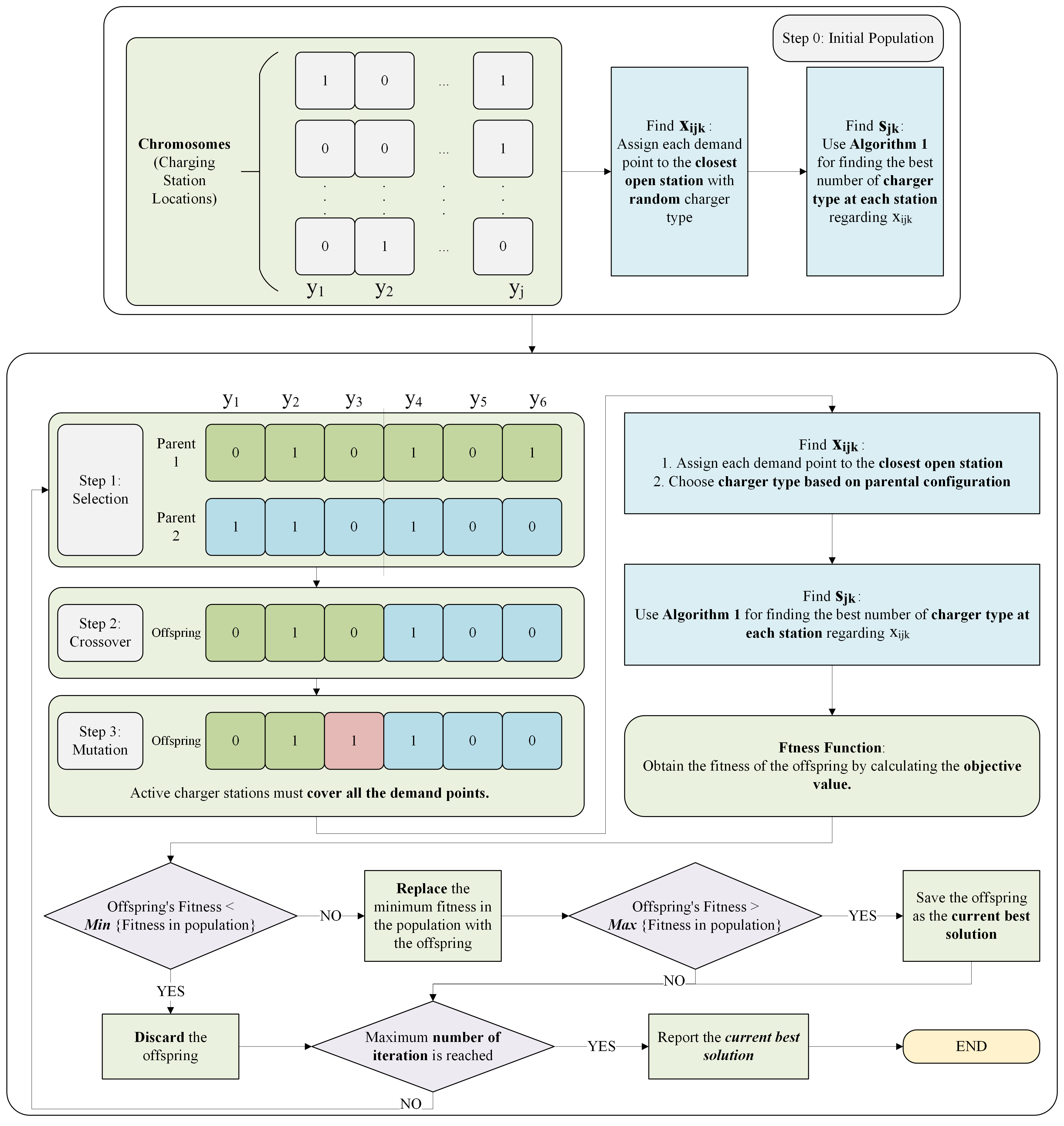
Figure 4: The Genetic Algorithm layout

fig]fig_GA

4.3 Simulated Annealing

SA is another metaheuristic method inspired by the cooling process of melted metals [24]. We utilize two main parameters for SA: the initial temperature $T_{0}$ and the maximum number of iterations $L$. Below are the steps of the SA algorithm for solving this problem:

1. Initialize:

   • Set the temperature $T$ to $T_{0}$ and the number of iterations $l$ to zero.

   • Identify the subset of active charging stations ($y_{j}=1$) using LABEL:minstations, denoted as current stations ($\mathcal{J}^{current}$).

   • Calculate $x_{ijk}$ and $s_{jk}$ for the current stations using LABEL:s_given_x.

   • Determine the objective value of the current stations and set the best solution to it: $\mathbb{C}^{best}=\mathbb{C}^{current}$ and $\mathcal{J}^{best}=\mathcal{J}^{current}$.

2. Make a move:

   • Create the subset of new stations ($\mathcal{J}^{new}$) by randomly closing one of the active stations in current stations $\mathcal{J}^{current}$ or activating one of the closed stations.

   • Repeat this step until you find a feasible subset $\mathcal{J}^{new}$ (i.e., active stations can cover all demand points).

   • Calculate $x_{ijk}$, $s_{jk}$, and the objective value of the new stations ($\mathbb{C}^{new}$).

3. Check for new best solution:

   • If $\mathbb{C}^{new}<\mathbb{C}^{best}$:

     • Update the best solution to the new solution: $\mathcal{J}^{best}=\mathcal{J}^{new}$ and $\mathbb{C}^{best}=\mathbb{C}^{new}$.

     • Update the current solution to the new solution: $\mathcal{J}^{current}=\mathcal{J}^{new}$ and $\mathbb{C}^{current}=\mathbb{C}^{new}$.

   • Otherwise:

     • Calculate the metropolis acceptance criterion: $m=\frac{\mathbb{C}^{current}-\mathbb{C}^{new}}{T}$.

     • Generate a random number. If it is less than $m$, update the current solution to the new solution: $\mathcal{J}^{current}=\mathcal{J}^{new}$ and $\mathbb{C}^{current}=\mathbb{C}^{new}$.

4. Update temperature: $T=T\times\left(1-\frac{0.5T_{0}}{L}\right)$

5. Stopping criteria:

   • Increment the iteration count: $l=l+1$.

   • If the algorithm has reached the final iterations ($l=L$): Stop and report the best solution.

   • Otherwise ($l<L$): go to item 2.

Function MinStations($\mathcal{I}$, $\mathcal{I}_{j}$, $\mathcal{J}$):

       Initialize: $\mathcal{I}^{\psi}\leftarrow\mathcal{I}$, $\mathcal{J}^{\psi}\leftarrow\mathcal{J}$, $\mathcal{J}^{\min}\leftarrow\emptyset$;

      while $\mathcal{I}^{\psi}\neq\emptyset$, do

             $j\leftarrow\text{argmax}_{j\in\mathcal{J}^{\psi}}\lvert\mathcal{I}_{j}\rvert$; $\triangleright$ Get station $j$ with the highest number of $i\in\mathcal{I}_{j}$ ($j$ with min $C_{j}^{\phi}$ when tied)

            if $\sum_{k\in\mathcal{K}}(\mu_{k}\cdot\overline{S}_{jk})>\sum_{i\in\mathcal{I}_{j}}\lambda_{i}$ then

                   for $i^{\prime}\in\mathcal{I}_{j}\cap\mathcal{I}^{\psi}$ do

                         $\mathcal{I}^{\psi}\leftarrow\mathcal{I}^{\psi}\setminus\{i^{\prime}\}$; $\triangleright$ Remove $i^{\prime}$ from $\mathcal{I}^{\psi}$

                   end for

                  $\mathcal{J}^{\min}\leftarrow\mathcal{J}^{\min}\cup\{j\}$; $\triangleright$ Add $j$ to $\mathcal{J}^{\min}$

                  $\mathcal{J}^{\psi}\leftarrow\mathcal{J}^{\psi}\setminus\{j\}$; $\triangleright$ Remove $j$ from $\mathcal{J}^{\psi}$

             end if

            

       end while

      

return $\mathcal{J}^{\min}$ $\triangleright$ Smallest subset of stations for feasibility, and $\lvert\mathcal{J}^{\min}\rvert$ is the minimum number of stations.

algo]minstations

Algorithm 3 Smallest subset of stations for feasibility

5 Case Studies

Various data sources are integrated to craft the case study for deploying charging stations in Chicago, IL. Most of the necessary data, including trip schedules and locations of garages and stops, are publicly available through the General Transit Feed Specification (GTFS) [25]. We calculated deadhead travel times by assuming an average bus speed of 20 mph and using Manhattan distances. Seven CTA and ten PACE bus garages are considered as well as 1078 stop terminals as candidate charging stations. Other parametric details were provided in [18]. The problem in the base scenario, called baseline, is to decide how many chargers of what type should be allocated to each candidate station. LABEL:param_sum summarizes the parameters used in the baseline.

Table 3: Parameter Values of the Case Study

tab]param_sum

Parameter	Value	Source
BEB battery capacity	440 kWh	[8]
Vehicle energy consumption rate	3 kWh/mi	[5, 26]
BEB constant speed	20 mph	Assumed
‘Slow charger’ power	125 kW	[8, 18]
‘Fast charger’ power	450 kW	[8, 7, 18]
Station cost	208,000 $	[9]
‘Slow charger’ cost	55,500 $	[9]
‘Fast charger’ cost	200,000 $	[9]
Chargers lifetime	10 years	[17]
Facility lifetime	30 years	[7]
Cost of detour	2.67 $/min	Calculated [27]
Cost of charging	3.46 $/min	Calculated [27, 28]

According to [28], CTA buses accumulate 4,830,866 annual revenue hours, with operating expenses totaling $774,665,363. Hence, the hourly cost of a travel is determined by dividing the annual operating expenses by the annual revenue hours. For charging time, an additional cost related to energy, obtained from [27], will be added. Specifically, a charge of $0.79 per minute will supplement the travel cost.

We consider three levers to configure different scenarios:

1. Sharing facilities between agencies: This parameter indicates whether PACE and CTA, the transit agencies in Chicago, can share each other’s facilities for recharging.

2. Including stops as candidates: Similar to the first lever, this specifies whether trips’ terminal stops can be considered as candidate charging stations.

3. Including garages as candidates: This lever determines whether terminal garages are considered as candidate charging stations.

By adjusting these levers, we generate six scenarios:

• Scenario 1. “Separate & garage-only”: BEBs can only recharge in the garages, and agencies only use their own charging locations.

• Scenario 2. “Separate & other-only”: BEBs can only recharge in the stop terminals but not garages, and agencies only use their own charging locations.

• Scenario 3. “Separate & mixed”: BEBs can recharge in the garages or stop terminals, and agencies only use their own charging locations.

• Scenario 4. “Joint & garage-only”: BEBs can only recharge in the garages, and agencies can use charging locations of each other.

• Scenario 5. “Joint & other-only”: BEBs can only recharge in the stop terminals, and agencies can use charging locations of each other.

• Scenario 6. “Joint & mixed”: BEBs can recharge in the garages or stop terminals, and agencies can use charging locations of each other.

LABEL:GAScenarios_sum compares the results of these scenarios by showing the percentage increase in the objective value $\mathbb{C}$ relative to Scenario 6. It also includes the number of candidate charging stations ($\lvert\mathcal{J}\rvert$), the number of active stations ($\sum_{j\in\mathcal{J}}y_{j}$), the total number of slow and fast chargers ($\sum_{j\in\mathcal{J}}s_{j}^{k=slow}$ and $\sum_{j\in\mathcal{J}}s_{j}^{k=fast}$), the average waiting time across all stations and chargers ($\overline{W_{jk}}$) in minutes, and the average utilization rate across all stations and chargers ($\overline{\rho_{jk}}$) in each scenario.

Table 4: Summary of scenario results

tab]GAScenarios_sum

Scenario	% $\uparrow$ in $\mathbb{C}$ vs. Scenario 6	$\lvert\mathcal{J}\rvert$	$\sum_{j\in\mathcal{J}}y_{j}$	$\sum_{j\in\mathcal{J}}s_{j}^{k=slow}$	$\sum_{j\in\mathcal{J}}s_{j}^{k=fast}$	$\overline{W_{jk}}(min)$	$\overline{\rho_{jk}}(\%)$
(1) Separate & garage-only	13.6	17	9	17	40	0.23	24.7
(2) Separate & other-only	21.0	23	8	21	35	0.26	27.2
(3) Separate & mixed	3.0	40	20	13	57	0.36	19.6
(4) Joint & garage-only	2.1	17	9	7	41	0.21	26.1
(5) Joint & other-only	15.5	23	13	22	42	0.25	23.5
(6) Joint & mixed	-	40	20	15	52	0.41	20.4

The results indicate that a joint charging infrastructure deployment strategy compared to a separate one reduces the cost though increasing the average waiting time and the average utilization rate. While garage-only scenario leads to an increase in the cost of deployment, other-only scenario impacts the cost even worse. This highlights that transit agencies are targeting a more economical deployment strategy by prioritizing garage deployment and delaying charging infrastructure deployment to elsewhere. On the other hand, the solutions also depict the importance of a mixed deployment strategy. Briefly, joint and mixed deployment is the key to achieve a cost-friendly deployment of EV infrastructure.

6 Conclusion

In this paper, we propose an optimization model to address the challenge of optimally locating charging stations and allocating chargers considering the stochastic charging demand of BEBs. The relevant literature both from a methodological and application was reviewed, and the study’s contributions are clearly stated. An exact solution method based on the cutting-plane constraints was developed to address finding optimal solutions to reasonably-sized problems. Two metaheuristic solution methods, GA and SA, were developed to solve large-scale problem instances. The GA was ran on case studies with real-world data. The results showed that a collaborative and a spatially comprehensive deployment strategy leads to an economical solution.

Although this study makes some notable improvements over the existing literature, some aspects still remain for future work. One of the main limitations of this study is finding the demand points by placing dividers to an already existing schedule for diesel buses. The estimation of demand points is flawed due to the method of positioning dividers according to the schedule of diesel buses. This approach overlooks waiting and charging times for buses during the initial estimation of demand points. Additionally, aggregating demand over time lacks realism; a more accurate approach would involve categorizing the day and calculating demand for each time slot individually.

The submitted manuscript has been created by UChicago Argonne, LLC, Operator of Argonne National Laboratory (“Argonne”). Argonne, a U.S. Department of Energy Office of Science laboratory, is operated under Contract No. DE-AC02-06CH11357. The U.S. Government retains for itself, and others acting on its behalf, a paid-up nonexclusive, irrevocable worldwide license in said article to reproduce, prepare derivative works, distribute copies to the public, and perform publicly and display publicly, by or on behalf of the Government. The Department of Energy will provide public access to these results of federally sponsored research in accordance with the DOE Public Access Plan http://energy.gov/downloads/doe-public-access-plan.

References

- Perumal et al. [2022] Perumal, S. S., R. M. Lusby, and J. Larsen, Electric bus planning & scheduling: A review of related problems and methodologies. European Journal of Operational Research, Vol. 301, No. 2, 2022, pp. 395–413.
- Tzamakos et al. [2023] Tzamakos, D., C. Iliopoulou, and K. Kepaptsoglou, Electric bus charging station location optimization considering queues. International Journal of Transportation Science and Technology, Vol. 12, No. 1, 2023, pp. 291–300.
- Uslu and Kaya [2021] Uslu, T. and O. Kaya, Location and capacity decisions for electric bus charging stations considering waiting times. Transportation Research Part D: Transport and Environment, Vol. 90, 2021, p. 102645.
- Hsu et al. [2021] Hsu, Y.-T., S. Yan, and P. Huang, The depot and charging facility location problem for electrifying urban bus services. Transportation Research Part D: Transport and Environment, Vol. 100, 2021, p. 103053.
- McCabe and Ban [2023] McCabe, D. and X. J. Ban, Optimal locations and sizes of layover charging stations for electric buses. Transportation Research Part C: Emerging Technologies, Vol. 152, 2023, p. 104157.
- Gkiotsalitis et al. [2023] Gkiotsalitis, K., C. Iliopoulou, and K. Kepaptsoglou, An exact approach for the multi-depot electric bus scheduling problem with time windows. European Journal of Operational Research, Vol. 306, No. 1, 2023, pp. 189–206.
- Hu et al. [2022] Hu, H., B. Du, W. Liu, and P. Perez, A joint optimisation model for charger locating and electric bus charging scheduling considering opportunity fast charging and uncertainties. Transportation Research Part C: Emerging Technologies, Vol. 141, 2022, p. 103732.
- Chicago Transit Authority [2022] Chicago Transit Authority, Charging Forward: CTA Bus Electrification Planning Report. URL: https://www. transitchicago. com/assets/1/6/Charging_Forward_Report_2-10-22_ (FINAL). pdf, 2022.
- He et al. [2023a] He, Y., Z. Liu, and Z. Song, Joint optimization of electric bus charging infrastructure, vehicle scheduling, and charging management. Transportation Research Part D: Transport and Environment, Vol. 117, 2023a, p. 103653.
- Vendé et al. [2023] Vendé, P., G. Desaulniers, Y. Kergosien, and J. E. Mendoza, Matheuristics for a multi-day electric bus assignment and overnight recharge scheduling problem. Transportation Research Part C: Emerging Technologies, Vol. 156, 2023, p. 104360.
- Berman and Krass [2019] Berman, O. and D. Krass, Stochastic Location Models with Congestion. In Location Science (G. Laporte, S. Nickel, and F. Saldanha da Gama, eds.), Springer, Switzerland, 2019, chap. 17, pp. 477–531, ed.
- Sun et al. [2020] Sun, X., Z. Chen, and Y. Yin, Integrated planning of static and dynamic charging infrastructure for electric vehicles. Transportation Research Part D: Transport and Environment, Vol. 83, 2020, p. 102331.
- Xu and Meng [2020] Xu, M. and Q. Meng, Optimal deployment of charging stations considering path deviation and nonlinear elastic demand. Transportation Research Part B: Methodological, Vol. 135, 2020, pp. 120–142.
- He et al. [2018] He, J., H. Yang, T.-Q. Tang, and H.-J. Huang, An optimal charging station location model with the consideration of electric vehicle’s driving range. Transportation Research Part C: Emerging Technologies, Vol. 86, 2018, pp. 641–654.
- Rogge et al. [2018] Rogge, M., E. Van der Hurk, A. Larsen, and D. U. Sauer, Electric bus fleet size and mix problem with optimization of charging infrastructure. Applied Energy, Vol. 211, 2018, pp. 282–295.
- Wei et al. [2018] Wei, R., X. Liu, Y. Ou, and S. K. Fayyaz, Optimizing the spatio-temporal deployment of battery electric bus system. Journal of Transport Geography, Vol. 68, 2018, pp. 160–168.
- An [2020] An, K., Battery electric bus infrastructure planning under demand uncertainty. Transportation Research Part C: Emerging Technologies, Vol. 111, 2020, pp. 572–587.
- Davatgari et al. [2024] Davatgari, A., T. Cokyasar, O. Verbas, and A. K. Mohammadian, Heuristic solutions to the single depot electric vehicle scheduling problem with next day operability constraints. Transportation Research Part C: Emerging Technologies, Vol. 163, 2024, p. 104656.
- Winston [2004] Winston, W. L., Operations Research Application and Algorithms. Brooks/Cole—Thomson Learning, Belmont, CA, ed., 2004.
- Grassmann [1983] Grassmann, W., The convexity of the mean queue size of the M/M/c queue with respect to the traffic intensity. Journal of Applied Probability, Vol. 20, No. 4, 1983, pp. 916–919.
- Lee and Cohen [1983] Lee, H. L. and M. A. Cohen, A note on the convexity of performance measures of M/M/c queueing systems. Journal of Applied Probability, Vol. 20, No. 4, 1983, pp. 920–923.
- Cokyasar and Jin [2023] Cokyasar, T. and M. Jin, Additive manufacturing capacity allocation problem over a network. IISE Transactions, Vol. 55, No. 8, 2023, pp. 807–820.
- Gurobi Optimization, LLC [2024] Gurobi Optimization, LLC, Callbacks. Available at https://www.gurobi.com/documentation/current/refman/py_cb_s.html accessed on Feb. 29, 2024, 2024.
- Berman and Drezner [2007] Berman, O. and Z. Drezner, The multiple server location problem. Journal of the Operational Research Society, Vol. 58, No. 1, 2007, pp. 91–99.
- General Transit Feed Specification [2022] General Transit Feed Specification, GTFS Schedule Reference, 2022.
- He et al. [2023b] He, Y., Z. Liu, Y. Zhang, and Z. Song, Time-dependent electric bus and charging station deployment problem. Energy, Vol. 282, 2023b, p. 128227.
- US Bureau of Labor Statistics [2024] US Bureau of Labor Statistics, Average Energy Prices, Chicago-Naperville-Elgin. https://www.bls.gov/regions/midwest/news-release/averageenergyprices_chicago.htm, June 2024, [Accessed 15-05-2024].
- Federal Transit Administration [2022] Federal Transit Administration, 2022 Annual Agency Profile - Chicago Transit Authority. https://www.transit.dot.gov/sites/fta.dot.gov/files/transit_agency_profile_doc/2022/50066.pdf, 2022, [Accessed 15-05-2024].