Topological transitions in quantum jump dynamics:
Hidden exceptional points

Abstract

Complex spectra of dissipative quantum systems may exhibit degeneracies known as exceptional points (EPs). At these points the systems’ dynamics may undergo a drastic change. Phenomena associated with EPs and their applications have been extensively studied in relation to various experimental platforms, including, i.a., the superconducting circuits. While most of the studies focus on EPs appearing due to the variation of the system’s parameters, we focus on EPs emerging in the full counting statistics of the system. We consider a monitored three level system and find multiple EPs in the Lindbladian eigenvalues considered as functions of a counting field. We demonstrate that these EPs signify transitions between different topological classes which are rigorously characterized in terms of the braid theory. Furthermore, we identify dynamical observables affected by these transitions and demonstrate how the underlying topology can be recovered from experimentally measured quantum jump distributions. Additionally, we establish a duality between certain EPs in the Lindbladian with regard to the counting field. This allows for an experimental observation of the EP transitions, normally hidden by the Liouvillian dynamics of the system, at arbitrary times without applying postselection schemes.

I Introduction

Complex spectra of non-Hermitian operators may possess exceptional points (EPs) - degeneracies in eigenvalues with simultaneous coalescence of the corresponding eigenvectors [1, 2, 3, 4]. The presence of EPs can have drastic consequences for system’s properties in their vicinity, such as non-adiabatic switching [5, 6, 7], dynamical phase transitions [8, 9, 10, 11, 12, 13], quantum Zeno effect [14, 15, 16, 17], spontaneous symmetry breaking [18, 19, 20], topological phase transitions [21, 22, 23, 24, 25, 26]. These sudden changes in the system’s behaviour at the EP can be understood in the framework of the catastrophe theory [27, 28, 29] and originate from non-analyticities of the Riemann surfaces for complex eigenvalues as functions of the system’s parameters. Among the phenomena associated with EP transitions, the topological phase transitions, studied within the topological band theory [30, 31], stand apart. In addition to the dependence on the external parameters, which can be explicitly controlled, the bands’ EPs emerge there at specific values of the momentum. The whole spectrum of such a system is periodic over the Brillouin zone, though particular bands may have different periodicity, and is characterised by a set of integer topological invariants - a change of these invariants results in a topological phase transition which necessarily involves an EP [22].

In recent years, EPs have been extensively studied in the fields of quantum optics and quantum superconducting hardware, as they find multiple applications for sensing [32, 33], amplification [34, 35], optimal steering [36], and entanglement generation [37]. The description of such dissipative systems usually requires going beyond the Hamiltonian dynamics and employing the Lindbladian formalism. In this case, the experimental analysis of phenomena associated with EPs is challenging due to the fact that the steady state of the full Lindbladian cannot be involved in an EP [38]. Thus, only the decaying states can host EPs. It means that EP-related effects can be observed only in the transient dynamics of the system [39]. Consequently, the experimental studies of EPs in dissipative systems have to deal with this limitation, focusing on the Hamiltonian EPs. The latter emerge, e.g., in the postselection schemes, in which the effects of quantum jumps are suppressed. In particular such schemes allow accessing the systems’ dynamics conditioned on the temporal absence of quantum jumps [40, 41, 42]. Complementary, the dynamics of the system can be characterized in terms of the full counting statistics (FCS) of quantum jumps [43, 44, 45, 46], an approach well known within the field of mesoscopic transport. It allows identifying the quantum jumps probability distribution and its evolution in time. Within this approach, the spectrum of the system becomes a periodic function of the counting field. Interestingly, this spectrum can acquire non-trivial topological properties reminiscent of the topological band theory, as reported in [47] for a two-level system interacting with a detector.

In context of FCS, one usually resorts to studying the set of cumulants of the observable at hand. The work of Li et al. [47], followed by [48, 49], presents the challenge of studying and classifying the topologies that can occur in FCS. Such a classification should explicitly employ the emergent topological invariants. What we argue here is that to achieve a broad classification of the emergent topologies, knowledge of cumulants does not suffice. One needs to consider “hidden exceptional points”, that do appear at finite values of the counting fields. Our approach to topological classification presented here, which fuses between emergent topological invariants and the physics of hidden exceptional points, is followed by a detailed discussion, pointing out the possibility to obtain the necessary information from realistic (accuracy-limited) experimental sets of data.

In the present study, we investigate the behavior of a three-level dissipative system with monitored quantum jumps and address the open problems mentioned above. This research is inspired by the recent experiment [41] focused on detection and reversal of quantum jumps midflight in a three-level artificial atom realized using superconducting qubits.

The paper is structured in the following way. We summarize our main results in Section II. In Section III we introduce the model under consideration and discuss its relation to the existing experimental setups of superconducting qubits and trapped ions. We introduce the topological classification of the system, calculate the corresponding invariants and discuss their relation to the non-Abelian braid theory in Section IV. In Section V we discuss how the drastic changes in the vicinity of the EPs are related to the observables of the full counting statistics of quantum jumps. In Section VI, we discuss how these observables can be constructed from the typical experimental quantum jump histograms and illustrate how one can recover the underlying topology from these data. Finally, in Section VII, we propose a universal duality connection between the Lindbladian EPs at the zero and non-zero values of the counting field. In Section VIII we discuss the implications of this duality for observing Lindbladian EP dynamics at arbitrary times without using postselection as well as possible consequences for the error correction protocols.

II Main results

Here we briefly summarize the main findings of our research.

$\bullet$ We reveal a deep connection between the dynamics of quantum jumps and the topological band theory. Namely, we identify qualitatively different classes of time-dependent quantum jump distributions which are defined by topological structures of the Lindbladian eigenvalues considered as functions of the counting field for the quantum jumps. We establish the rigorous topological characterization of these dynamical classes in terms of the non-abelian braid theory and find an unexpectedly rich variety of non-trivial topological classes even in small systems. These classes are topologically protected, i.e. they are resilient against external perturbations and noise as long as these perturbations are not too strong.

$\bullet$ We demonstrate that transitions between different topological classes of quantum jumps occur through exceptional points of the system’s Lindbladian equiped with the jump-counting field.

$\bullet$ We identify a dynamical observable that is affected by these topological transitions and demonstrate how the underlying topological structures can be restored from quantum jump distributions collected in state-of-the-art experiments.

$\bullet$ We show that the analysis of the Lindbladian eigenvalues at the non-zero values of the counting field allows bypassing the no-go theorem that prohibits formation of EPs in the longest living Lindbladian eigenstate [38, 50]. Moreover, there is a duality between EPs of the Lindbladian eigenvalues at zero and half-period values of the counting field, so that these EPs appear in pairs. These findings provide tools for studying phenomena associated with EPs in the full Lindbladian picture without employing any postselection protocols.

Our results show the role of the EPs in formation of the non-Poissonian quantum jump statistics and establish a connection between non-equilibrium dynamics and the underlying topological characterization of dissipative systems, demonstrating that dynamical phase transitions are, in fact, topological transitions. They provide tools for studying phenomena associated with EPs in the full Lindbladian picture without dependence on postselection protocols.

III Model

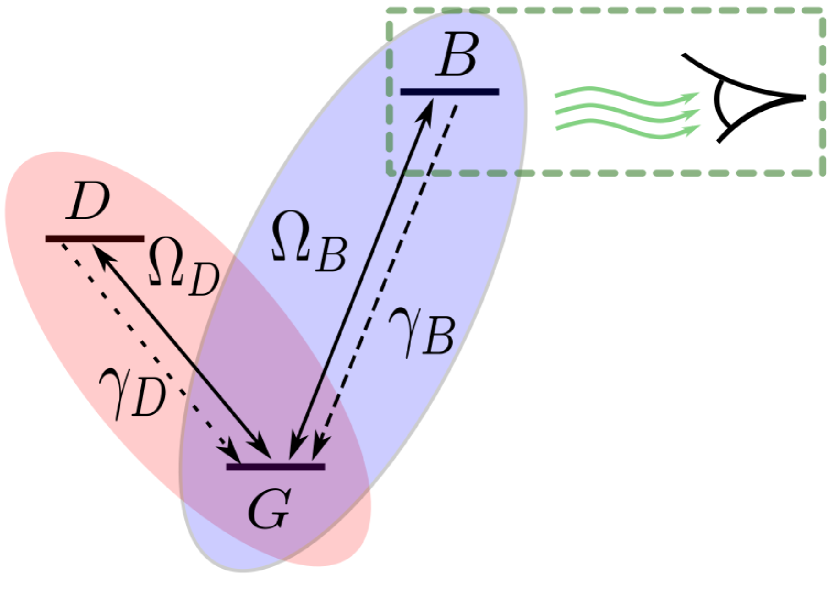
Figure 1: A cartoon picture of the three level system under consideration. The bright state (B) is continuously monitored and quickly decays into the ground state (G). The dark state (D) is not monitored. The Rabi drives $\Omega_{B}$ and $\Omega_{D}$ induce transitions between $G\rightleftharpoons B$ and $G\rightleftharpoons D$ states, respectively. $\gamma_{B}\gg\gamma_{D}$ are decay rates.

Superconducting qubits have become one of paradigmatic platforms for experimental studies of quantum jumps. Over recent years, quantum jumps occurring in such systems have been successfully observed and controlled in various experiments [51, 52, 53, 41, 42, 54, 55]. We consider a setup that closely matches the dissipative three level system studied in [41]. In particular, we focus on the fluorescent quantum jump measurements [56, 57, 58] model described there. This setup is reminiscent of earlier observations of quantum jumps in trapped ions with fluorescence detection [59, 60, 61, 62]. Namely, we consider a three level $V$-shaped system comprised of the ground (G), bright (B) and dark (D) states. Its schematic representation is shown in Fig. 1. This system is known to exhibit dynamical phase transitions between a rich variety of dynamical phases [63, 64, 65, 66]. The bright state relaxes spontaneously at a very high rate into the ground state, this relaxation process is constantly monitored, while the dark state is not monitored at all. In addition, there are two periodic real Rabi drives $\Omega_{D}$ and $\Omega_{B}$ which enable transitions between $G\rightleftharpoons D$ and $G\rightleftharpoons B$ states, respectively. The detailed derivation of the effective three-level Hamiltonian from two coupled qubits under resonant driving is given in Appendix A. The effective three-level description in the interaction picture with the rotating wave approximation is given by

$$H_{I}=\Omega_{D}S^{x}+\Omega_{B}T^{x},$$ (1)

$S^{x}=\frac{1}{2}(S^{+}+S^{-}),\,T^{x}=\frac{1}{2}(T^{+}+T^{-})$, where $S^{\pm}$ and $T^{\pm}$ are $3\times 3$ matrices that form raising and lowering operators in the basis $\{\ket{G},\ket{D},\ket{B}\}$. They account for transitions between $G\rightleftharpoons D$ and $G\rightleftharpoons B$ states correspondingly:

$$S^{+}=\begin{pmatrix}0&0&0\\ 1&0&0\\ 0&0&0\end{pmatrix},\,\,\,T^{+}=\begin{pmatrix}0&0&0\\ 0&0&0\\ 1&0&0\end{pmatrix},$$ (2)

$$S^{-}=\,\left(S^{+}\right)^{\dagger},\,\,\,\,\,\,\,\,\,\,\,\,\,\,T^{-}=\,\left(T^{+}\right)^{\dagger}.$$ (3)

The decay from exited states $B$ and $D$ into the ground state $G$ can be accounted by the dissipators $T^{-}$ and $S^{-}$ with respective rates $\gamma_{B}$ and $\gamma_{D}$. We assume that the bright state B decays at a very high rate, while the dark state D is almost lossless. These assumptions are motivated by the experimental situation of [41], where $\gamma_{B}\gg\Omega_{B}\gg\Omega_{D}\gg\gamma_{D}$. We keep the same hierarchy throughout our manuscript. Due to the introduced dissipation, the dynamics of the system is non-Hermitian. Without quantum jumps, this evolution can be described by the effective non-Hermitian Hamiltonian:

$$H_{eff}=H_{I}-\frac{\textit{i}}{2}\gamma_{D}T^{+}T^{-}-\frac{\textit{i}}{2}\gamma_{B}S^{+}S^{-}.$$ (4)

The full Lindbladian operator of the system includes this effective Hamiltonian part and the quantum jump operators. Since the bright state decay is constantly monitored, each decay from the bright state into the ground state, which is accompanied by emission of a photon, is detected. Such a transition is modelled by a quantum jump term, and therefore one have direct access to the statistics of the $B\rightarrow G$ quantum jumps throughout measurements. We add the counting field $k$ to the corresponding jump term of the Lindladian to reproduce this experimentally accessible FCS. In the superoperator notations ([67, 38]), the resulting Lindbladian reads:

$$\mathcal{L}_{k}=-\textit{i}\left\{\left(H_{I}-\frac{\textit{i}}{2}\Gamma^{\dagger}\Gamma\right)\otimes\mathbb{1}-\mathbb{1}\otimes\left(H_{I}^{T}+\frac{\textit{i}}{2}\Gamma^{T}\Gamma^{*}\right)\right\}$$

$$+\gamma_{B}e^{\textit{i}k}\,T^{-}\otimes T^{-}+\gamma_{D}S^{-}\otimes S^{-},$$ (5)

where we denoted $\Gamma^{\dagger}\Gamma\equiv\gamma_{B}T^{+}T^{-}+\gamma_{D}S^{+}S^{-}$. $\otimes$ denotes the Kronecker product, superscripts $T$ and $*$ stand for transposition and complex conjugation. Note that the full Lindbladian is periodic with respect to the counting field $k$, which is a direct consequence of an integer number of detected events. With this Lindbladian, the density matrix evolves as

$$\rho_{k}(t)=e^{\mathcal{L}_{k}t}\rho_{0},$$ (6)

where $\rho_{k}(t)$ is the dynamically evolving density matrix that depends of the counting field $k$. More precisely, $\rho_{k}(t)\equiv\sum_{n}e^{-ink}\rho_{n}(t)$ is the Fourier image of $\rho_{n}(t)$ - the density matrix of the system conditioned by $n$ quantum jumps exhibited over the measurement time $t$. Its trace gives the probability to observe exactly $n$ quantum jumps, $P_{n}(t)=Tr[\rho_{n}(t)]$. In principle, one can analyze this density matrix $\rho_{k}$ directly, performing the full state tomography. Instead, we focus on a situation that is more relevant for experiments - detecting only occurrences of the quantum jumps, without knowledge of the full structure of the density matrix. For further use, we introduce the Fourier transform $P_{k}(t)$ of the probability $P_{n}(t)$ to observe $n$ quantum jumps over time $t$:

$$P_{k}(t)=\sum_{n}e^{ikn}P_{n}(t)=\left\langle e^{\textit{i}kn}\right\rangle(t)=Tr\left[e^{\mathcal{L}_{k}t}\rho_{0}\right]\ .$$ (7)

$$P_{n}(t)=\int_{0}^{2\pi}\frac{dk}{2\pi}e^{-\textit{i}nk}P_{k}(t),$$ (8)

these probabilities can be gathered during multiple repetitions of the experiment.
For simplicity, we put $\gamma_{D}=0$ throughout the paper, assuming that there is no decay from the dark state and $G\rightleftharpoons D$ transitions happen only due to the $\Omega_{D}$ drive. We discuss the $\gamma_{D}\neq 0$ case in Section VII. For numerical calculations, unless specified otherwise, we choose $\gamma_{B}=0.5,\,\Omega_{B}=0.1$ in dimensionless units (i.e. with respect to some characteristic frequency of the system). Some of the present results depend quantitatively on the choice of these parameters, while others are universal, as we specify below.

IV Topological invariants

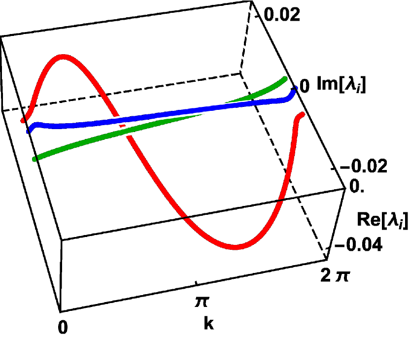
$\Omega_{D}<\Omega_{3}$

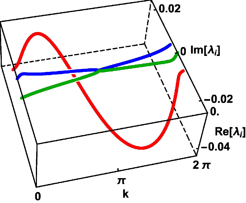
$\Omega_{D}=\Omega_{3}$

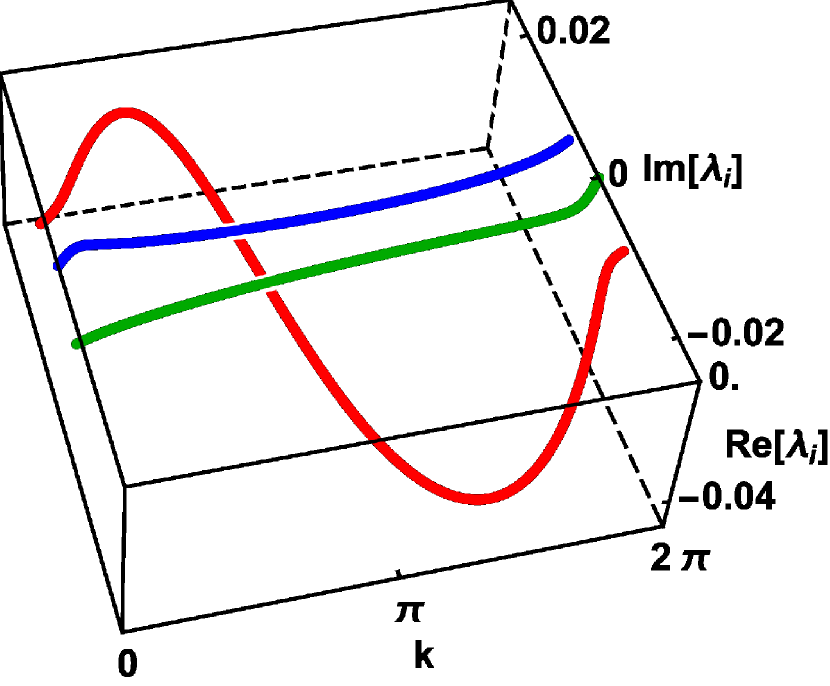
$\Omega_{D}>\Omega_{3}$

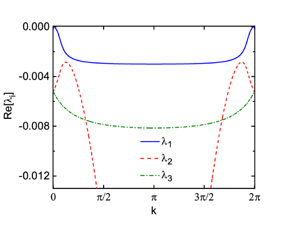
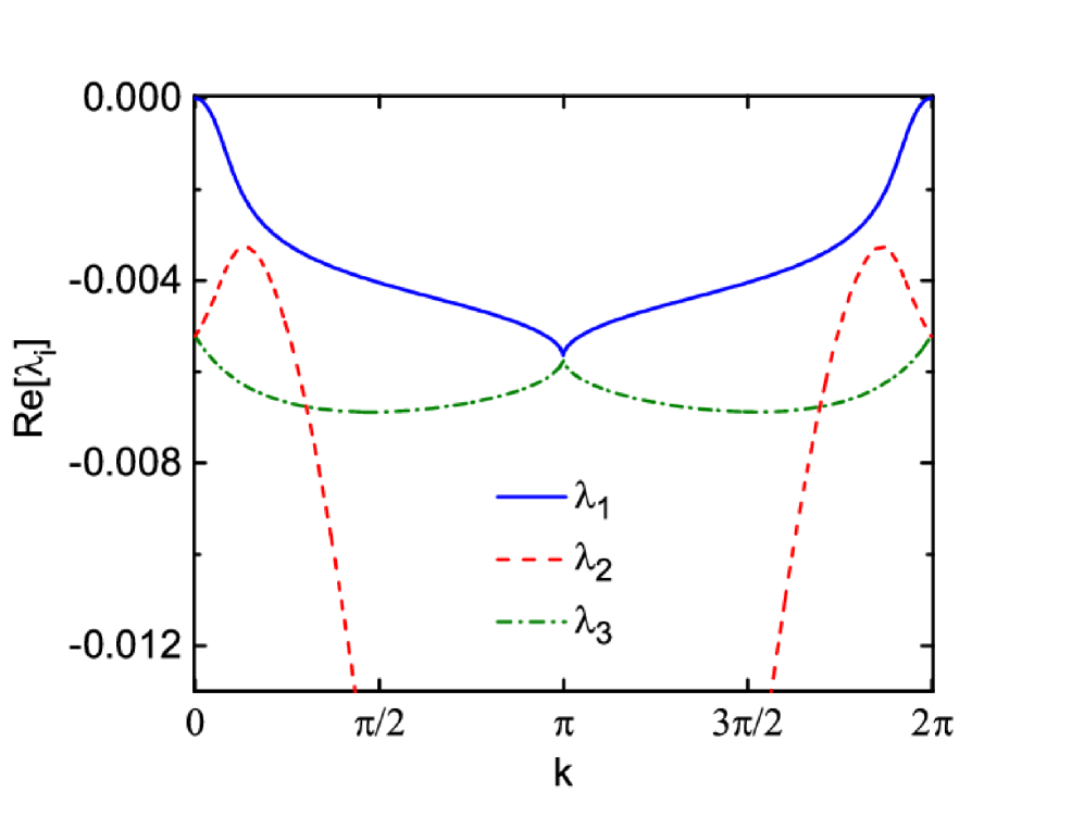
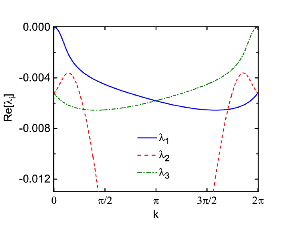
Figure 2: Examples of two different eigenvalue braids and a transition between them. The transition between two classes results in an EP at $k=\pi$. Upper panel: Real and imaginary structure of the three least decaying eigenvalues of the Lindbladian Eq. 5 as functions of the counting field $k$ at different values of the drive $\Omega_{D}$. Lower panel: Real parts of the corresponding eigenvalues. The transition occurs with variation of the drive $\Omega_{D}$. $\Omega_{3}$ is the critical frequency specified below (Table 2).

Since the real counting field $k$ acts as a phase for the jump term in Eq. 5, the Lindblad operator is $2\pi$-periodic over $k$, $\mathcal{L}_{k}=\mathcal{L}_{k+2\pi}$. The same applies to its spectrum. Nevertheless, a particular eigenvalue of the Lindbladian is not necessarily $2\pi$-periodic, as eigenvalues can swap their positions during the $2\pi$ circling. Moreover, even if the eigenvalues are $2\pi$-periodic, they still may wind around each other. A qualitative change in this winding structure means a change in the system’s topology. Such structures and transitions between them can be described by means of the braid theory. One can switch between different braids by a proper change of the system’s parameters [68, 69, 70, 71]. For Hamiltonian systems stochastically interacting with a detector, the topological braids can appear the same way in full counting statistics [72, 47, 48, 49], and EPs can emerge at non-zero values of the counting field [73]. Below, we demonstrate that the same applies to the Lindbladian EPs. Moreover, the change in eigenvalues’ braid structure with respect to the counting field necessarily results in a change in the system’s topology even if periodicity of the eigenvalues is unaffected. Similar to the results of the topological band theory, the qualitative changes in braid structures, and the subsequent topological transitions, occur when the system passes through an EP.
We consider braids of eigenvalues of the Lindbladian Eq. 5 as functions of the counting field $k$. In particular, out of nine eigenvalues of this Lindbladian, we focus on three eigenvalues with smallest decay rates (i.e. three eigenstates with smallest real parts at $k=0$). The forth one does not contain dependence on $k$ and does not change its braiding with respect to other eigenvalues at any parameters; other five eigenvalues have much higher decay rates, so they are separated from the former ones by a large gap, which prevents them from participating in braids with the long-living eigenstates. Braids of these three eigenvalues correspond to $B_{3}$ braid group. The periodicity of the eigenvalues over $k$ means that the braids are closed, and the knot theory provides an equivalent description [74, 75, 7]. We will not delve into details of the braid and knot theories, referring to reviews on the subjects [76, 77, 78], but rather use some basic results from them, which are summarized in Appendix B.
We illustrate the braid structure of the considered eigenvalues in Fig. 2, where the upper panels show how a change in the external parameter $\Omega_{D}$ results in a change in periodicity of the complex eigenvalues. This change happens through an EP at the particular drive value $\Omega_{D}=\Omega_{3}$ (specified below). The lower panels show the real parts of the eigenvalues, corresponding to the eigenstates’ decay rates.
Let us introduce the braid index for two Lindbladian complex eigenvalues $\lambda_{a}$ and $\lambda_{b}$, similar to the braid index used for characterization of topological bands [68, 69]:

$$\nu^{(a,b)}=\int_{0}^{2\pi}\frac{dk}{2\pi\textit{i}}\frac{d}{dk}\log\left[\frac{\lambda_{a}(k)-\lambda_{b}(k)}{2}\right].$$ (9)

class	$\,\,\,\nu\,\,\,$	$\nu_{a;b}$	braid word
I	4	$\nu_{1;2}=2$, $\nu_{1;3}=2$	$\sigma_{1}\sigma_{2}\sigma_{2}\sigma_{1}$
II	2	$\nu_{2;3}=2$	$\sigma_{2}\sigma_{2}$
III	1	$\nu_{2;3}=1$	$\sigma_{2}$
IV	2	-	$\sigma_{2}\sigma_{1}$
V	0	-	$\mathbb{1}$

Table 1: Different topological classes corresponding to different braids of eigenvalues Eq. 5 with respect to the counting field $k$. Each class is characterised by its topological index $\nu$ and a set of its invariants, which can be related to a unique braid word.

transition	$\Omega_{i}$ ($i=1..4$)	$k$
I - II	0.00230	0.02825*
II - III	0.00521	0
III - IV	0.00779	$\pi$
IV - V	0.03147	2.70492*

Table 2: Parameters of the exceptional points. Each EP corresponds to a specific change in topology of the system. There are four EPs separating five different classes. ^∗ denotes that for a given frequency $\Omega_{D}=\Omega_{i}$, the same exceptional point is present also at $2\pi-k$, since the eigenvalues are $2\pi$-periodic in $k$ and invariant under translations $k\rightarrow-k$.

We denote further

$$\nu_{a;b}=\nu^{(a,b)}+\nu^{(b,a)};$$ (10)

$$\nu_{a,b;c}=\nu^{(a,c)}+\nu^{(c,a)}+\nu^{(b,c)}+\nu^{(c,b)};$$ (11)

$$\nu_{a;b,c}=\nu^{(a,b)}+\nu^{(b,a)}+\nu^{(a,c)}+\nu^{(c,a)};$$ (12)

$$\nu=\sum_{i<j}\left(\nu^{(i,j)}+\nu^{(j,i)}\right).$$ (13)

The integer topological invariant $\nu$ counts the total braid degree of the class. This index can coincide for different topologically distinct classes, so other indexes allow for more nuanced description. This is aligned with the fact that $B_{3}$ braid group is non-abelian and hence cannot be characterized by a single parameter. $\nu_{a;b}$ shows the relative braid degree between eigenvalues $a$ and $b$. $\nu_{a,b;c}$ shows the braid degree of two eigenvalues $a$ and $b$ with respect to the third eigenvalue $c$ ($\nu_{a;b,c}$ acts in the similar way, showing the braid degree of one eigenvalue with regard to the other two). The indexes accounting for braiding of more than two eigenvalues become important when periodicity of some eigenvalues differs from $2\pi$ and these eigenvalues braid with $2\pi$-periodic eigenvalues, since $\nu_{a;b}$ is unable to provide a meaningful result in this case accounting for integration over only a part of the full period of the eigenvalues (though this particular situation does not happen in our system for the three chosen eigenvalues).

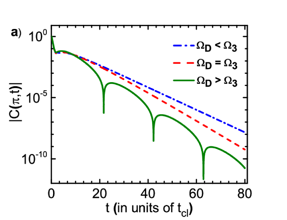
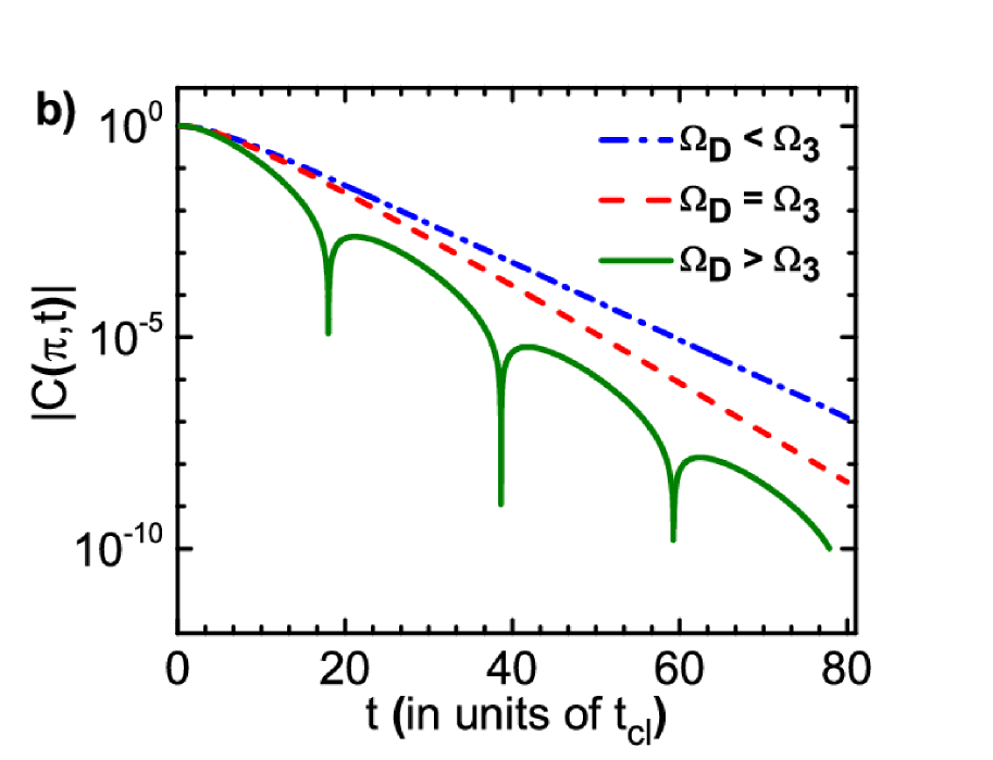
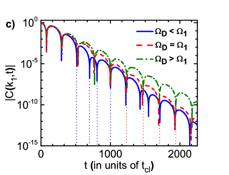
Figure 4: $C(k,t)$ and transitions of its dynamics corresponding to topological transitions between different topological classes. a and b: $k=\pi$, the transition between III and IV classes of Table 1. Passing through the EP, $C(\pi,t)$ changes its behavior between purely exponential decay and exponential decay with oscillations (note the $\log$ scale). Dash-dotted blue line - $\Omega_{D}<\Omega_{3}$ ($\Omega_{D}=0.0075$), i.e. the system is in the class III; solid green line - $\Omega_{D}>\Omega_{3}$ ($\Omega_{D}=0.009$), i.e. the system is in the class IV; dashed red line - $\Omega_{D}=\Omega_{3}$, exceptional point. a: The system is initially prepared in the ground (G) state; b: The evolution starts from the dark (D) state. c: Transition between classes I and II. $k_{1}=0.02825$ is taken from Table 2, the system is initially prepared in the ground state. Blue solid line - $\Omega_{D}<\Omega_{1}$ ($\Omega_{D}=0.00225$) ; red dashed line - $\Omega_{D}=\Omega_{1}$, green dash-dotted line - $\Omega_{D}>\Omega_{1}$ ($\Omega_{D}=0.00235$). $C(k_{1},t)$ changes its behavior at the EP between decay with harmonic oscillations and decay with a beating pattern; the vertical blue and red dotted lines show the change in the oscillations periodicity. Time t is in units of the inverse transition rate to the bright state $t_{cl}=\Gamma_{B}^{-1}$.

For chosen parameters (see Section III), we identify five different topological classes listed in Table 1 and shown in Fig. LABEL:fig:phases, where we draw the braid diagrams of each class along with a knot equivalent to this periodic braid diagram. Each color represents variation of a particular eigenvalue over $2\pi$. These classes are separated by four exceptional points listed in Table 2. Note that, similarly as it happens with non-Hermitian eigenvalues braids of Bloch bands [69], our braids of eigenvalues can be defined on a period $[k_{0},k_{0}+2\pi]$ of the counting field with an arbitrary initial point $k_{0}$, so the braid words given in Table 1 are defined up to cyclic permutations. As one should expect from the topological nature of these classes, they are protected against infinitesimal perturbations of the external parameters of the system. Namely, while exact values of $\Omega_{D}$ and $k$ listed in Table 2, where the EPs emerge, strongly depend on all parameters’ values, the overall structure of these transitions remains robust. For instance, it takes a sufficient change in $\gamma_{D}$ to remove the class I from the system, though other phases are robust even to a large change of this parameter, as is discussed in more details in Section VII.

V Observable dynamical properties

After we established the topological nature of the considered system, we are interested in identifying a physical observable that is affected by these topological features, so one can identify the occurring topological transitions in experiments. Usually, braiding occurs when some Hamiltonian parameters are varied (e.g. driving frequencies) so that the direct observation of the associated dynamical phase transitions or encircling the associated EP is possible. In contrast, in our case, there is no way to directly change the counting field $k$ which has a statistical nature. Despite this, we show that one still can choose a time dependent observable that distinguishes different classes (at least some of them) in experiments.
Let us consider the Fourier transform $P_{k}(t)$ of the probability to observe $n$ quantum jumps over time $t$, which is given by Eq. 7. Expanding in the basis of eigenvectors of $\mathcal{L}_{k}$, and assuming that we are not at an EP (though we may be infinitesimally close to it), we obtain

$$P_{k}(t)=Tr\left[\sum_{j}e^{\lambda_{k}^{(j)}t}\ket{\chi_{k}^{(j),R}}\innerproduct{\chi_{k}^{(j),L}}{\rho_{0}}\right],$$ (14)

where $\ket{\chi_{k}^{(j),R}}$ and $\bra{\chi_{k}^{(j),L}}$ are the right and left eigenvectors corresponding to the complex eigenvalue $\lambda^{(j)}_{k}$ of the Lindbladian $\mathcal{L}_{k}$ given by Eq. 5 at fixed $k$ (they are well-defined as long as we are not exactly at an EP). Above, we used

$$\innerproduct{\chi_{k}^{(i),L}}{\chi_{k}^{(j),R}}=\delta_{ij},\,\,\,\sum_{i}\ket{\chi_{k}^{(i),R}}\bra{\chi_{k}^{(i),L}}=1.$$ (15)

While taking the trace in Eq. 14, one should convert $\ket{\chi_{k}^{(j),R}}$ from superoperator notations back to the matrix representation. In what follows we will investigate

$$C(k,t)=Re[P_{k}(t)]=\left\langle\cos\left(kn\right)\right\rangle(t)\ .$$ (16)

In analogy to the qualitative analysis of the Lindblad operator in Ref. [41], we introduce the characteristic rate of the $G\rightleftharpoons B$ transitions, $\Gamma_{B}$, so that the characteristic time of one quantum jump (click) observation is given by $t_{cl}=\Gamma_{B}^{-1}$. The characteristic decay rate of the longest living state is denoted by $\Gamma_{D}$. One easily obtains

$$\Gamma_{B}=\frac{\Omega^{2}_{B}}{\gamma_{B}},\,\,\,\Gamma_{D}=\frac{\Omega^{2}_{D}}{\Gamma_{B}}=\gamma_{B}\frac{\Omega^{2}_{D}}{\Omega^{2}_{B}}.$$ (17)

As we will argue below, our formalism allows observing the EP transitions if the EP involves the longest lived states. In Fig. 4 we show two such transitions. The exponential decays present in Fig. 4 behave as $e^{-\alpha\Gamma_{D}t}$, with $\alpha$ being a non-universal number ${\cal O}(1)$. As we show in Fig. 4, crossing an EP that involves the longest living eigenstate of the Lindbladian results in a drastic change of the observable $C(k,t)$. The transition III-IV shown in (a) and (b) of Fig. 4 corresponds to the transition illustrated in Fig. 2, namely, the braid of two eigenvalues with smallest decay rates changes there, changing the periodicity of these eigenvalues. This immediately results in a transition of $C(\pi,t)$ from pure exponential decay (Class III) into decay with oscillations (Class IV). The physical meaning of $C(\pi,t)$ can be simply understood. Since $P_{k}(t)$ is the Fourier transform of $P_{n}(t)$, which is the probability to observe $n$ jumps over time $t$, $C(0,t)=1$ has a simple interpretation: $P_{k=0}(t)=\sum_{n=0}^{\infty}P_{n}(t)=1$, namely, the probabilities to observe all numbers of quantum jumps are summed into $1$. At $k=\pi$, $C(\pi,t)$ also has a straightforward interpretation

$$P_{k=\pi}(t)=\sum_{n=0}^{\infty}e^{\textit{i}\pi n}P_{n}(t)=\sum_{n=even}P_{n}(t)-\sum_{n=odd}P_{n}(t),$$ (18)

i.e. it’s the difference between probabilities to observe even and odd number of jumps over time $t$.
In Class IV, $C(\pi,t)$ slowly changes its sign, so at different times it is more probable to observe either even or odd number of quantum jumps. This non-trivial structure of the quantum jump probabilities originates from the non-Poissonian distribution of quantum jumps. We analyze this distribution in more details in Appendix C. In short, the interplay between $G\rightleftharpoons B$ and $G\rightleftharpoons D$ transitions, which independently would be Poissonian and characterized by $\Gamma_{B}$ and $\Gamma_{D}$ rates, creates this effective non-Poissonian distribution with parity of jumps that oscillates in time. Further, Fig. 4(c) shows the $\textit{I}-\textit{II}$ transition from Table 2. Note that in this transition none of the involved eigenvalues changes its periodicity. Nevertheless, the braid of the eigenvalues changes, and the changed topology (namely, a transition between a connected sum of two Hopf links to a Hopf link with an unlink, specified in Fig. LABEL:fig:phases) manifests in the change of the behavior of $C(k,t)$. At the EP, in addition to a usual exponential decay with the $\Gamma_{D}$ rate, the time evolution of $C(k,t)$ switches between harmonic oscillations and a beating pattern.
Note that $C(k,t)$ does not require any postselection, as all occurred jumps contribute to this observable. Nevertheless $C(k,t)$ at $k=\pi$ and $k=k_{1}$ (given in the first raw of Table 2) identify the EP transitions at arbitrary long times. Other transitions listed in Table 2 cannot be clearly observed through the dynamical behavior of $C(k,t)$, as they involve states with higher decay rates and the EP dynamical transition becomes masked by the dynamics of the longer lived states, the same way as it normally happens for the Lindbladian dynamics at $k=0$. In Section VII, we show that, nevertheless, there is an innate connection between the "unobservable" EP at $k=0$ and the one at $k=\pi$ which we analyzed above.

VI Retrieving the topology from experimental jump distributions

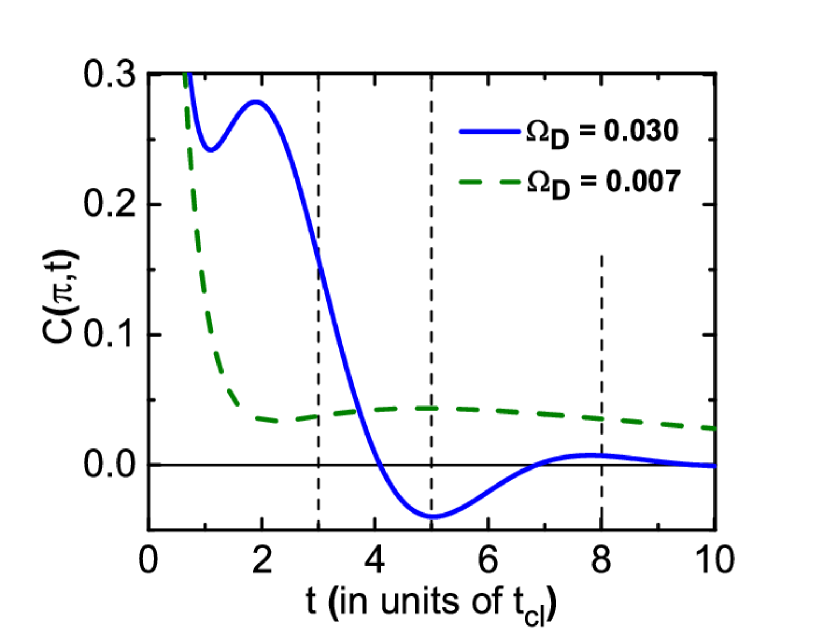
Figure 5: $C(\pi,t)$ on two sides of the $\textit{III}-\textit{IV}$ transition. Solid blue line - oscillatory behavior at $\Omega_{D}>\Omega_{3}$, green dashed line - pure decay at $\Omega_{D}<\Omega_{3}$. The initial state is G.

In this section we discuss in more details how the underlying topology of the system can be extracted from $P_{k}(t)$ obtained from experimentally gathered distributions of quantum jump probabilities. The Lindbladian eigenvalues separated from the longest-living state by a non-zero Liouvillian gap give exponentially small contributions to Eq. 7 comparing to the leading terms. As a result, restoring all the eigenvalues from the jump distributions gathered during the experiment would require fitting $P_{k}(t)$ by nine complex decaying exponents and nine complex prefactors, which does not seem plausible. Nevertheless, one can still distinguish different topological structures of Fig. LABEL:fig:phases whenever at least the two longest decaying eigenstates are topologically different. We focus on the transition between classes III and IV, as the most robust case. This particular transition is also most suited for experimental studies since it always happens at the fixed $k=\pi$ (as we discuss in the next section), rather than at some accidental value of $k$. We choose the ground state G ($\rho_{0}=\ket{G}\otimes\ket{G}$) as the initial state. This is a reasonable choice, since immediately after each jump the system is reliably in the G state. Every such point can be chosen as the starting time for the observations.

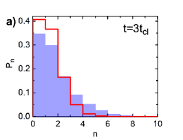
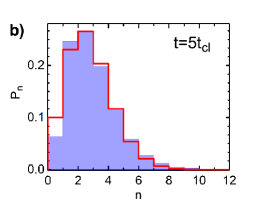
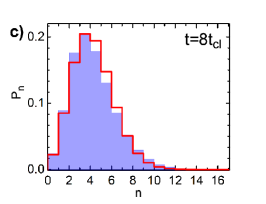
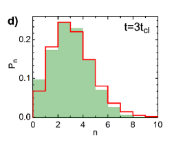
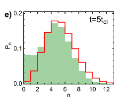
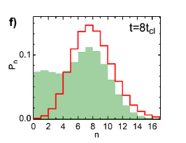
Figure 6: Distributions of quantum jumps at fixed times $3t_{cl}$ (a, d), $5t_{cl}$ (b, e), $8t_{cl}$ (c, f) (vertical dashed lines in Fig. 5). a-c: $\Omega_{D}=0.03\gg\Omega_{3}$, oscillatory regime. d-f: $\Omega_{D}=0.007<\Omega_{3}$, pure decay. Red histograms show closest Poissonian distributions.

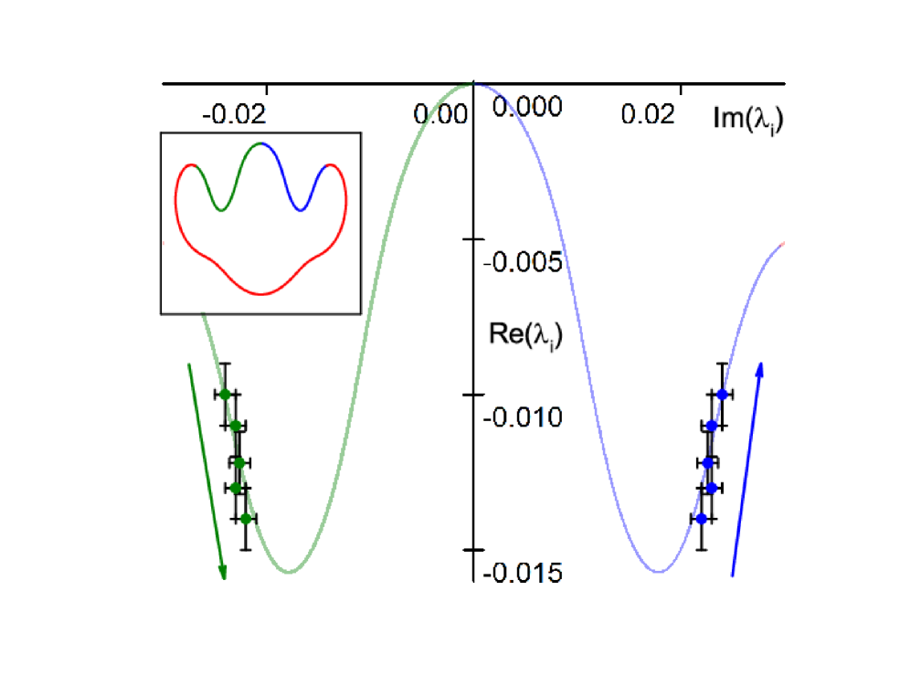
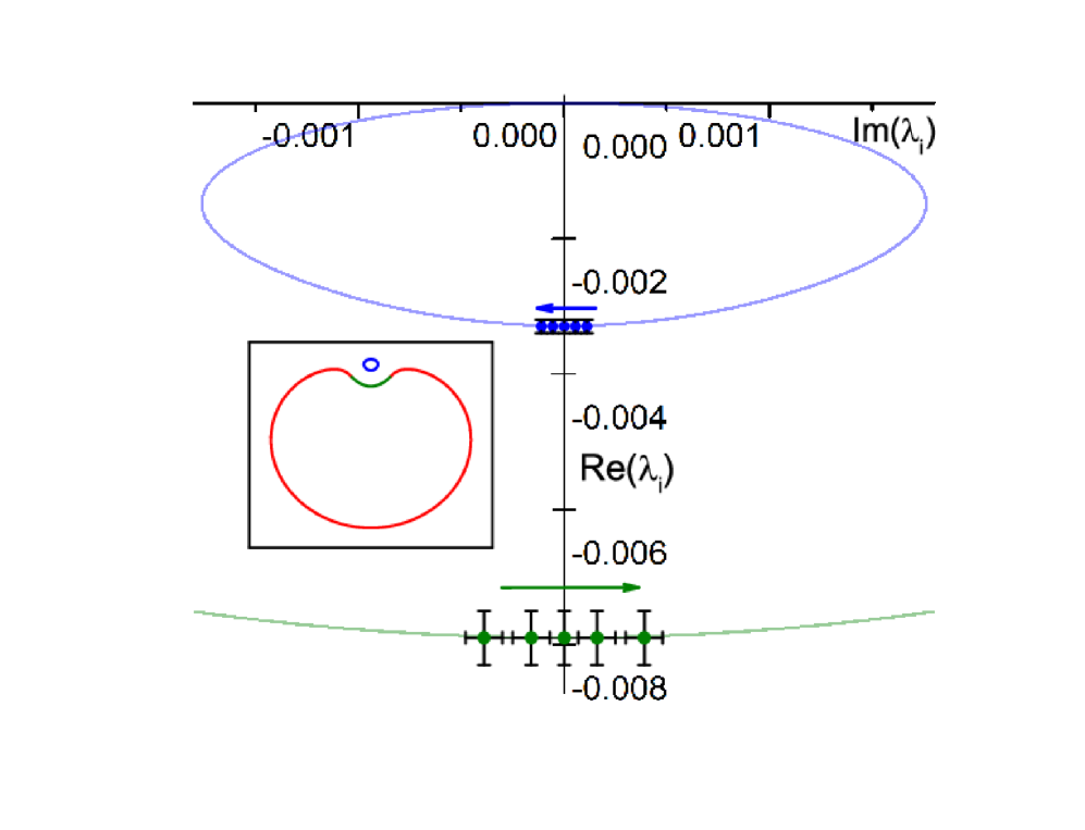
Figure 7: Parametric plots of imaginary ($x-$axis) and real ($y-$axis) parts of eigenvalues $\lambda_{k}^{(1)}$, $\lambda_{k}^{(2)}$ depending on $k$. Left panel - $\Omega_{D}=0.03$, right panel - $\Omega_{D}=0.007$. Blue and green dots are fits for $P_{k}(t)$ through Eqs. 21, 22. Background solid blue and green lines - exact values for these eigenvalues. Values of $k$ are $\pi-0.4,\,\pi-0.2,\,\pi,\,\pi+0.2,\,\pi+0.4$, arrows show movement directions of the eigenvalues with increase of $k$. Insets: The same, zoomed-out, parametric plots showing topological structures for the three leading eigenvalues as $k$ changes from $0$ to $2\pi$.

Since many quantum jumps contribute to the observable $C(\pi,t)$ and the resulting sum decays in time exponentially, from the practical perspective, the observation time should be kept relatively small ($t/t_{cl}\sim 10^{0}-10^{2}$). We illustrate it in Fig. 5, which reflects the same transition as in Fig. 4(a), namely, the regime $\Omega_{D}=0.03$ which belongs to Class IV far away from the excectional point (so the oscillations of $P_{k}(t)$ are easier to spot) and the regime $\Omega_{D}=0.007$ of Class III, where the sign of $P_{k}(t)$ is always positive. Away from the EP, the difference of imaginary parts of the eigenvalues forming that EP grows, increasing the oscillations’ frequency, and making them easier to spot. In Fig. 6, we plot the distributions of quantum jumps taken at three different times, corresponding to vertical dashed lines in Fig. 5. It is worth noting here that in experiments with superconducting qubits such statistics can be easily gathered for an arbitrary number of points in time and with at least $\sim 10^{5}$ repetitions [55] at each point in time, so the finite size effects are almost neglidgible for the histograms in Fig. 6. We compare these distributions with best fit Poissonian distributions (red lines) to highlight the non-Poissonian character of jumps in both regimes. In the oscillatory regime (upper panels), despite the fact that the distributions follow the overall shape of the Poissonian distribution, they are qualitatively different. Indeed, small deviations from the Poissonian statistics accumulate to the oscillatory behavior of the staggered probability $C(\pi,t)$. In contrast, the Poissonian statistics always produces monotonous positive staggered probabilities $C^{P}(\pi,t)$. In particular, we have $C(\pi,3t_{cl})\simeq 0.158$, $C(\pi,5t_{cl})\simeq-0.040$, $C(\pi,8t_{cl})\simeq 0.007$, and $C^{P}(\pi,3t_{cl})\simeq 0.165$, $C^{P}(\pi,5_{t_{cl}})\simeq 0.010$, $C^{P}(\pi,8t_{cl})\simeq 0.005$. In the pure decay regime ($\Omega_{D}<\Omega_{3}$), the distributions are clearly non-Poissonian, as they are biased towards small $n$ contributions. Nevertheless, this regime always produces positive staggered probabilities $C(\pi,t)$: $C(\pi,3t_{cl})\simeq 0.038$, $C(\pi,5t_{cl})\simeq 0.043$, $C(\pi,8t_{cl})\simeq 0.035$.

We now discuss how the complex eigenvalues of the Lindbladian can be retrieved from the quantum jump probability distributions collected at different times. Taking the Fourier transform of the distributions $P_{n}(t)$ with respect to $n$, we obtain the probabilities $P_{k}(t)$ depending on the counting field $k$. For $k=\pi$, they reduce to functions plotted in Fig. 5. Using Eq. 14, we can write

$$P_{k}(t)=\sum_{i}C^{(j)}_{k}e^{\lambda_{k}^{(j)}t},$$ (19)

where $C_{k}^{(j)}$ are complex constants that depend on the eigenvectors and the initial conditions. We neglect all contributions from the fast decaying modes and approximate this expression as

$$P_{k}(t)\simeq C^{(1)}_{k}e^{\lambda_{k}^{(1)}t}+C^{(2)}_{k}e^{\lambda_{k}^{(2)}t}.$$ (20)

Assuming that the second exponent has a larger negative real part, we see that the first term dominates at longer times, so we can approximate

$$\log P_{k}(t)\simeq\log C^{(1)}_{k}+\lambda_{k}^{(1)}t+\frac{C_{k}^{(2)}}{C_{k}^{(1)}}e^{(\lambda_{k}^{(2)}-\lambda_{k}^{(1)})t}.$$ (21)

The last term is exponentially small comparing to the linear one, so we can neglect it for now and approximate $\log P_{k}(t)$ by a linear fit, finding real and imaginary parts of $\lambda_{k}^{(1)}\pm\delta\lambda^{(1)}_{k}$ and $C_{k}^{(1)}\pm\delta C_{k}^{(1)}$ for a chosen $k$. $\delta\lambda_{k}^{(1)}$ and $\delta C_{k}^{(1)}$ are small errors accumulated during this procedure. Next, we find the difference between two eigenvalues, present in the exponent Eq. 21, by subtracting the established leading contributions

$$\log\left[\log\frac{P_{k}(t)}{C_{k}^{(1)}}-\lambda_{k}^{(1)}t\right]\simeq\log\frac{C_{k}^{(2)}}{C_{k}^{(1)}}+(\lambda_{k}^{(2)}-\lambda_{k}^{(1)})t$$ (22)

$$+\frac{\delta C_{k}^{(1)}+\delta\lambda_{k}^{(1)}t}{\log P_{k}(t)-\log C_{k}^{(1)}-\lambda_{k}^{(1)}t}-\delta\lambda_{k}^{(1)}t-\frac{\delta C_{k}^{(1)}}{C_{k}^{(k)}}.$$ (23)

Here Eq. 22 allows finding $\lambda_{k}^{(2)}$ from a linear fit of the left-hand side, while Eq. 23 accounts for errors accumulated through this procedure due to $\delta\lambda_{k}^{(1)}$ and $\delta C_{k}^{(1)}$, while leads to increased errors in $\delta\lambda_{k}^{(2)}$ and $\delta C_{k}^{(2)}$. We implement this procedure and plot the retrieved values $\lambda_{k}^{(1)}$ and $\lambda_{k}^{(2)}$ for various $k$ in Fig. 7 for both regimes to illustrate that it indeed allows restoring the underlying topology of the eigenvalues.

VII Duality between Exceptional Points in Full Counting Statistics

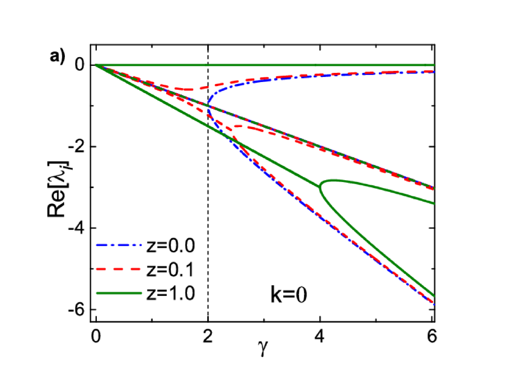
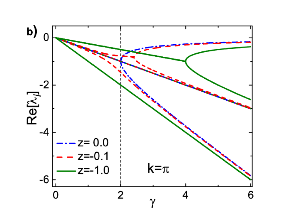
Figure 8: Exceptional point of the Lindbladian $L_{0}$ perturbed by the jump term $L_{J}$, Eq. 24 (this particular example is given by Eq. 26) with phases a) $k=0$ and b) $k=\pi$. Real parts of the Lindbladian eigenvalues $\lambda_{i}$ are plotted as functions of the parameter $\gamma$. $z=re^{\textit{i}k}$. Blue dot-dashed line is the unperturbed exceptional point structure $r=0$, red dashed line corresponds to the suppressed jumps case $r=0.1$, green solid line denotes the full jump term $r=1$. Vertical dashed black line highlights the critical value of $\gamma$ for the unperturbed exceptional point.

As proven in [38], the stationary state of the full Lindbladian operator cannot participate in the formation of an EP. This theorem relies on the fact that the trace of this state must be conserved. However, this reasoning can no longer be applied to the Lindbladian taken at non-zero counting field $k\neq 0$, since none of its eigenstates preserves the full trace anymore. We show in this section that in some cases one can use the so-called staggered cumulants [73] with $k=\pi$, or more generally $C(k,t)$, to unveil EPs which are normally hidden in the fast decaying modes at $k=0$. This duality can be established analytically for two level systems in the following way.
Let us consider an arbitrary two level system with a non-Hermitian Hamiltonian $H_{nH}=H-\frac{i}{2}\Gamma^{\dagger}\Gamma$ (here $H$ is Hermitian and $\Gamma$ is an arbitrary dissipator) which depends on a parameter $\gamma$ (e.g. it may be included in the dissipator $\Gamma$) and exhibits an exceptional point at some critical value of this parameter, $\gamma_{C}$. The introduce a modified Lindblad operator that takes form

$$\mathcal{L}=L_{0}+zL_{J},$$ (24)

$$L_{0}=-\textit{i}\left\{\left(H-\frac{\textit{i}}{2}\Gamma^{\dagger}\Gamma\right)\otimes\mathbb{1}-\mathbb{1}\otimes\left(H^{T}+\frac{\textit{i}}{2}\Gamma^{T}\Gamma^{*}\right)\right\}.$$ (25)

Here $L_{0}$ is the Lindbladian without quantum jumps, $L_{J}=\Gamma\otimes\Gamma^{*}$ is the jump term of the Lindbladian (here we use the superoperator notations), $z$ is a complex parameter with $|z|\in[0,1]$ that suppresses the weight of the jump contribution. $z=0$ corresponds to the purely Hamiltonian evolution without quantum jumps, $z=1$ restores the full Lindbladian evolution. $0<|z|<1$ corresponds to a hybrid-Liouvillian with suppressed contribution of quantum jumps that accounts for an imperfect detector [50]. Additionally, this parameter can have a non-zero phase, which corresponds to the non-zero counting field, similar to Eq. 5. Let us put $|z|\ll 1$, so the jump term $L_{J}$ in the Lindbladian Eq. 24 can be considered as a small perturbation for $L_{0}$. The second order EP of the non-Hermitian Hamiltonian $H_{nH}$ occurring at some parameter’s value $\gamma_{C}$ translates into the third order EP of the Lindbladian $L_{0}(\gamma_{C})$, as shown in Appendix D.

The effects of a small perturbation on the Lindbladian eigenvalues in the vicinity of the third order EP can be tracked analytically. Following the analysis of [27, 79, 80], we show in Appendix D how a general perturbation at $k=0$ splits three degenerate eigenvalues into a pair forming a perturbed EP of the second order and an isolated eigenvalue that does not participate in any EP. This isolated eigenvalue is the longest living, i.e. it has the smallest negative real part (smallest decay rate) of all eigenvalues, and becomes stationary in the limit $z=1$. By changing the sign of the jump term (i.e. adding the counting field with $k=\pi$), one inverses this order. We stress out that this behavior of EP perturbations is general for dissipative two level systems and does not rely on any additional assumptions.

We illustrate this principle for a dissipative two level system

$$H_{nH}=\frac{\omega}{2}\sigma^{x}-\textit{i}\frac{\gamma}{2}\sigma^{+}\sigma^{-},\,\,\,L_{J}=\gamma\sigma^{-}\otimes\sigma^{-},$$ (26)

which was used in [50] to study effects of perturbations on the EP by partially suppressed quantum jumps for the case of zero phase $k=0$. The behavior of the eigenvalues is shown in Fig. 8(a). On the contrary, the order of eigenvalues is inverted at $k=\pi$, so the same Liouvillian exceptional point forms now between two least decaying states, as shown in Fig. 8(b). This allows observing the EP in the decaying modes, which is normally hidden by the stationary mode. We stress out that although at $k=\pi$ the eigenstates hosting the EP are exponentially decaying, their decay is slowest comparing to all other modes, so they give the leading contribution to $C(k,t)$ (with other modes decaying exponentially faster), and transitions of the $C(k,t)$ dynamics (Eq. 16), similar to those in Fig. 4, can be observed.

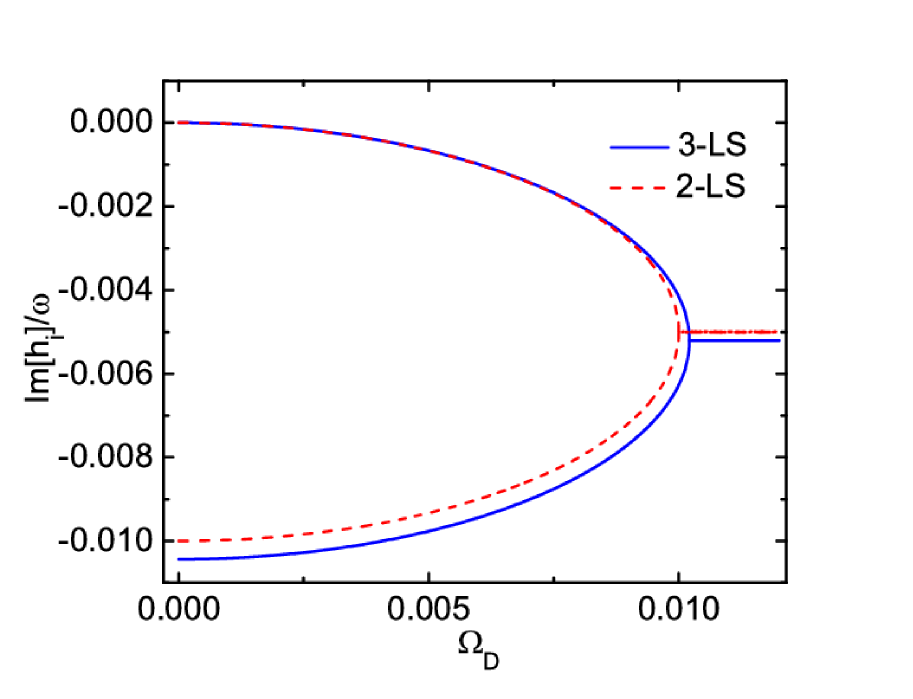
Figure 9: Eigenvalues $h_{i}$ (imaginary parts) of the three level system Hamiltonian Eq. (4) (blue solid lines, 3-LS) and eigenvalues of the effective G-D two level system’s Hamiltonian obtained via adiabatic elimination (red dashed line, 2-LS) as functions of the driving frequency $\Omega_{D}$. For the three level system, only two relevant eigenvalues (long-living states forming an exceptional point) are plotted. The reduced system retains the EP of the same structure in close proximity to the original EP.

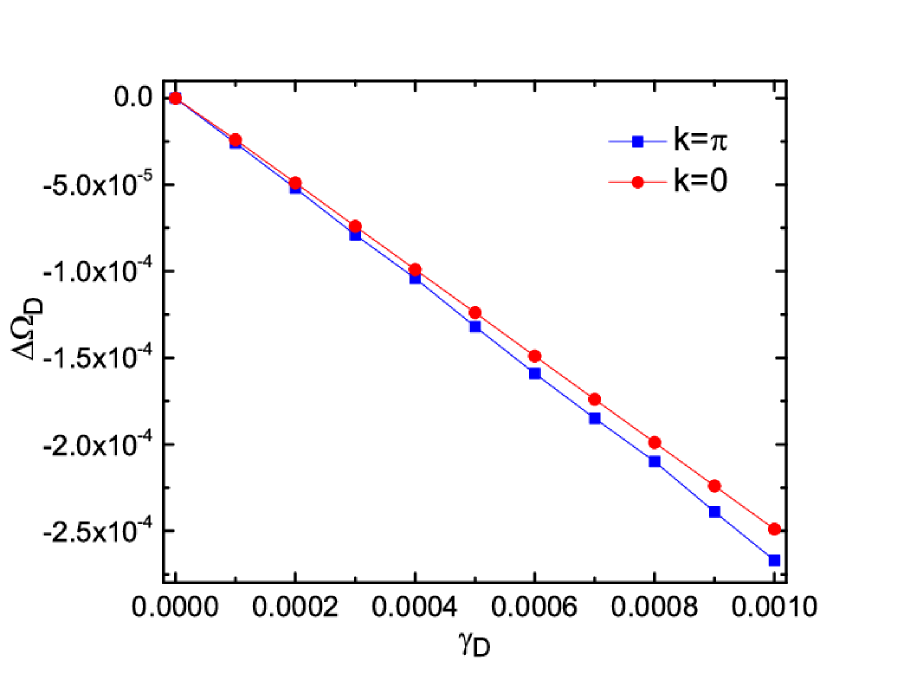
Figure 10: Change in the critical driving frequency $\Omega_{D}$ for the EP of the full Lindbladian Eq. 5 as a function of the dark stay decay $\gamma_{D}$ for $k=0$ (blue squares) and $k=\pi$ (red dots). The $y-$axis shows change in this frequency $\Delta\Omega_{D}=\Omega_{D}(\gamma_{D})-\Omega_{D}(0)$, where the critical driving frequencies $\Omega_{D}(0)$ for the corresponding $k$ are given in Table 2.

For a system with more than two states, the situation becomes more complicated and the $0-\pi$ duality of the EPs in different modes, strictly speaking, does not necessarily hold. Nevertheless, when the non-Hermitian Hamiltonian of the system hosts a second-order EP in its two least decaying states and all other states are substantially separated from them, one can use the adiabatic elimination method [81, 82, 83, 84, 85, 86, 87] to reduce the problem to an effective two level system preserving the EP. We discuss this procedure in details in Appendix E. For the three level system under consideration, with one state exhibiting very fast decay, the reduced two level system faithfully reproduces the EP of the non-Hermitian Hamiltonian Eq. 4, as illustrated at Fig. 9. The same procedure can be performed on the full Lindbladian, effectively reducing the description from nine to four eigenstates. The quantum jump term of the full Lindbladian perturbs the reduced Lindbladian eigenvalues in a non-trivial way. Nevertheless, a general expansion in terms of the jump amplitude discussed in Appendix D still holds, so at least for $|z|\ll 1$ case the stricture of the perturbed eigenvalues must be preserved. As we show numerically in Appendix E, the perturbed eigenvalues still exhibit the $0-\pi$ duality in $k$ for the EPs, though now they do not necessarily emerge at the same values of the driving frequency $\Omega_{D}$. This duality is the reason why in Table 2 there is a pair of EPs corresponding to $\textit{II}-\textit{III}$ and $\textit{III}-\textit{IV}$ transitions exactly at $k=0$ and $k=\pi$. This is illustrated in Fig. 10, where we consider various dark state decay rates $\gamma_{D}$ - though the change of this parameter shifts the frequencies $\Omega_{D}$ for the EP, the values $k$ of the two EPs remain fixed - there are always EPs at $k=0$ and $k=\pi$. This is not true for two other EPs listed in Table 2, where the values of $k$ are incidental and very sensitive to any changes in the parameters of the problem. For instance, the class I (and the subsequent transition $\textit{I}-\textit{II}$) completely disappears for substantially large $\gamma_{D}$ values, so the transitions that do not involve changes of the eigenvalues periodicity show lesser resilience to perturbations.

VIII Discussion and perspectives

We have analyzed the dissipative Lindbladian dynamics of a V-shaped three-level-system comprised of the ground, dark and bright states with monitored $B\rightarrow G$ quantum jumps. By drawing an analogy with topological band theory, we identify distinct topological classes of FCS, corresponding to different braids of complex eigenvalues of the Lindbladian. The qualitatively different quantum jump distributions of these classes are topologically protected, as infinitely small perturbations of the system’s parameters do not affect the braid structure. It takes a finite change of the system’s parameters (comparable to the scale of the distance between the eigenvalues) to change the integer braid index of the system and induce a topological transition. Transitions between the topological classes necessarily happen through exceptional points emerging at specific values of the counting field.

We have introduced the dynamical observable $P_{k}(t)$ which allows to identify transitions between different topological classes at arbitrary times as long as the corresponding EP involves the eigenvalues with the smallest decay rates. Such analysis of the EPs at non-zero values of the counting field $k$ provides an exception the theorem prohibiting formations of EPs in the Lindbladian eigenvalues that dominate at long times [38]. Some of these EPs are dual, i.e., they are located at special values of $k$ and necessarily emerge in pairs ($0$ - $\pi$). This duality allows for observation of the EP at $k=\pi$ at long times. Moreover, it allows for establishing an immediate relation to the $k=0$ EP of the conventional trace-preserving Lindbladian, which is concealed at long times by the presence of a trace preserving eigenstate. This approach has an advantage of neither requiring any postselection techniques nor monitoring particular eigenstates nor employing other highly selective measurements of the system, relying solely on counting the number of quantum jumps as a function of time.

Following the measurements, the histograms describing the numbers of quantum jumps that occur over a given time can be analyzed by means of the Fourier transform. This analysis provides meaningful information about the underlying EP structure and the topological class of the system. In other words, by appropriately fitting $P_{k}(t)$ as a function of time, one can restore the leading eigenvalues and their topological structure. We have demonstrated that for realistic, experiment-limited data sets, such retrieval of the topological structures can be done with reasonable accuracy provided sufficient resolution in time and sufficiently long-time statistics of the measurements. Both of these requirements are not a problem for state-of-the-art experimental setups of superconducting qubits, where quantum jump traces can be collected at high measurement rates and up to arbitrary long times over multiple experimental repetitions. Nevertheless, as large numbers of quantum jumps contribute to the $P_{k}(t)$ observable at long times, the noise and measurement imperfections have higher impact on the precision of the fit in this case. Hence, it is preferable to retrieve the topological structures of the Lindbladian eigenvalues not too close to the exceptional points, so that the distinct topology can be clearly seen already at relatively early observation times.

We argue that the developed approach to the dynamics of quantum jumps is quite general and can be applied to an analysis of any system exhibiting quantum jumps. It would be interesting to see how this approach can be related to other monitored quantum system, e.g. [88, 89]. In this work we concentrated on the second order EPs, as they are most common among all EP types. The overall reasoning about transitions in topological structures and the dynamics of the system should be applicable to higher order EPs and even to exceptional lines and exceptional surfaces. If there are several types of quantum jumps in a system, one can introduce several different counting fields and employ the same analysis for higher dimensional topological bands.

Our approach connects dynamical phase transitions to underlying topological transitions in a wide class of dissipative systems. It may turn out to be particularly useful for understanding emergent non-Poissonian errors in quantum processors, which is crucial for error correction protocols [90, 91, 92]. Understanding the eigenvalues topology in such systems may allow regulating transitions between Poissonian and non-Poissonian distributions of quantum jumps. Hence, potential opportunities emerge for topologically protecting the Poissonian structure of quantum jumps (and therefore ensuring the uncorrelated nature of errors) against emergent correlated errors.

Appendix A Effective three-level system

The system under consideration can be constructed with two physical qubits. We use Pauli matrices $\vec{\sigma}$ to denote the first qubit, and $\vec{\tau}$ to denote the second qubit. Their frequencies are $\varepsilon$ and $\omega$ correspondingly. The qubits are coupled longitudinally with the coupling constant $\chi$,

$$H_{0}=\frac{1}{2}\left(\varepsilon\sigma^{z}+\omega\tau^{z}+\chi\sigma^{z}\tau^{z}\right).$$ (27)

We encode the four states written in $\{\ket{\sigma,\tau}\}$ basis as

$$\ket{G}=\ket{\downarrow\downarrow},\,\ket{D}=\ket{\uparrow\downarrow},\,\ket{B}=\ket{\downarrow\uparrow},\,\ket{F}=\ket{\uparrow\uparrow}.$$ (28)

The state $\ket{F}$ is an auxiliary one, corresponding to both qubits being excited. In principle, it can be used to account for all higher energy excited states of the two qubit system in experimental realizations [41]. The eigen-energies of the Hamiltonian (27) (counting from the ground state, so $E_{G}\equiv 0$) are given by

$$E_{D}=\varepsilon-\chi,\,E_{B}=\omega-\chi,\,E_{F}=\varepsilon+\omega.$$ (29)

One applies harmonic Rabi drives with frequencies $\varepsilon-\chi$ and $\omega-\chi$ to induce Rabi transitions $\ket{G}\rightleftharpoons\ket{D}$ and $\ket{G}\rightleftharpoons\ket{B}$. With an appropriate choice of $\chi$, the state $\ket{F}$ can be sufficiently detuned, so it does not participate in these transitions. The full Hamiltonian reads

$$H=H_{0}+H_{drive},$$ (30)

$$H_{drive}=\Omega_{D}\cos\left((\varepsilon-\chi)t\right)\sigma^{x}+\Omega_{B}\cos\left((\omega-\chi)t\right)\tau^{x}.$$ (31)

The possible phase shifts of both drives are ignored as they do not affect the results. Now, we obtain the effective three-level system Hamiltonian. For this, we transform to the interaction picture

$$H_{I}=e^{\textit{i}H_{0}t}H_{drive}e^{-\textit{i}H_{0}t}.$$ (32)

Using

$$\sigma^{x}_{I}=e^{\textit{i}(\varepsilon+\chi\tau^{z})t}\sigma^{x},\,\,\,\tau^{x}_{I}=e^{\textit{i}(\omega+\chi\sigma^{z})t}\tau^{x},$$ (33)

and 31, we obtain

$$H_{I} =\Omega_{D}\cos\left((\varepsilon-\chi)t\right)e^{\textit{i}(\varepsilon+\chi\tau^{z})}\sigma^{x}+$$

$$+\Omega_{B}\cos\left((\omega-\chi)t\right)e^{\textit{i}(\omega+\chi\sigma^{z})}\tau^{x}.$$ (34)

Operators 33 act on our four states 28 in the following way:

$$e^{\textit{i}(\varepsilon+\chi\tau^{z})t}\sigma^{x}\ket{G}=e^{\textit{i}(\varepsilon-\chi)t}\ket{D},$$ (35)

$$e^{\textit{i}(\varepsilon+\chi\tau^{z})t}\sigma^{x}\ket{D}=e^{-\textit{i}(\varepsilon-\chi)t}\ket{G},$$ (36)

$$e^{\textit{i}(\varepsilon+\chi\tau^{z})t}\sigma^{x}\ket{B}=e^{\textit{i}(\varepsilon+\chi)t}\ket{F},$$ (37)

$$e^{\textit{i}(\varepsilon+\chi\tau^{z})t}\sigma^{x}\ket{F}=e^{-\textit{i}(\varepsilon+\chi)t}\ket{B},$$ (38)

$$e^{\textit{i}(\omega+\chi\sigma^{z})t}\tau^{x}\ket{G}=e^{\textit{i}(\omega-\chi)t}\ket{B},$$ (39)

$$e^{\textit{i}(\omega+\chi\sigma^{z})t}\tau^{x}\ket{B}=e^{-\textit{i}(\omega-\chi)t}\ket{G},$$ (40)

$$e^{\textit{i}(\omega+\chi\sigma^{z})t}\tau^{x}\ket{D}=e^{\textit{i}(\omega+\chi)t}\ket{F},$$ (41)

$$e^{\textit{i}(\omega+\chi\sigma^{z})t}\tau^{x}\ket{F}=e^{-\textit{i}(\omega+\chi)t}\ket{D}.$$ (42)

Substituting these expressions into Eq. 34, we see that there are time dependent oscillating terms and time independent ones. We apply the rotating-wave approximation to keep only the latter, which brings us to the effective Hamiltonian written in Eq. 1 with operators

$$S^{+}=\ket{D}\bra{{G}},\,\,\,T^{+}=\ket{B}\bra{{G}},$$ (43)

$$S^{-}=\left(S^{+}\right)^{\dagger},\,\,\,T^{-}=\left(T^{+}\right)^{\dagger},$$ (44)

which can be represented in the form of Eqs. 2, 3.
Note that these terms do not allow transitions involving the auxiliary state $F$, effectively reducing the four level system to the three-level $V$-shaped one. The non-Hermitian terms in Eq. 4 commute with $H_{0}$, so they do not change in the interaction picture.

Appendix B Basics of braid and knot theories

Here we collect some basic results and methods from the theory of closed braids that we use in the main part. Throughout the paper, we consider braids composed of three strands, their braid group is $B_{3}$, though all our results can be straightforwardly applied to $B_{n}$ braid group describing $n$ strands. The non-trivial elements of $B_{3}$ braid group are given in Fig. 11: each $\sigma_{i}$ element accounts for braiding between $i$ and $i+1$ strands (counted from above). It is $\sigma_{i}$ if the strand $i$ goes above $i+1$ and $\sigma_{i}^{-1}$ otherwise. In our case, there are only four braid elements: $\sigma_{1}$, $\sigma_{1}^{-1}$, $\sigma_{2}$, $\sigma_{2}^{-1}$ (and additionally the identity element $\mathbb{1}$ when no braiding is performed). A sequential application of these elements allows creating any possible braid pattern for three strands. A resulting sequence of braidings is called the braid word.

$\sigma_{1}$

$\sigma_{1}^{-1}$

$\sigma_{2}$

$\sigma_{2}^{-1}$

Figure 11: Elementary braid elements of $B_{3}$ braid group for three strands.

The theory allows for homological representations, so the braid elements can be written in matrix form. In the reduced Burau representation [76] of $B_{3}$ braid group, the non-trivial elements are given by matrices

$$\sigma_{1}=\begin{pmatrix}t&1\\ 0&1\end{pmatrix},\,\,\,\sigma_{2}=\begin{pmatrix}1&0\\ -t&t\end{pmatrix}.$$ (45)

We note in passing that this homological representation is known to be faithful for $B_{3}$ (i.e. it is a one-to-one representation of the braid group), so it suffices for us. For extension of this analysis to $B_{n}\,(n>3)$, other representations, although more complicated, may be preferable.
In Eq. 45, we can choose $t\in(0,1)$ to reflect the fact that our $B_{3}$ braid group is not cyclic:

$$\forall m\in\mathbb{Z}:\,\,\,\sigma_{i}^{m}\neq\mathbb{1},\,\,\,(\sigma_{i}\sigma_{j}\sigma_{i})^{4m}\neq\mathbb{1}.$$ (46)

Other rules for braid operations are as follows:

$$...\sigma_{i}\sigma_{i}^{-1}...=...\mathbb{1}...\,,$$ (47)

$$...\sigma_{1}\sigma_{2}...\neq...\sigma_{2}\sigma_{1}...\,,$$ (48)

$$...\sigma_{1}\sigma_{2}\sigma_{1}...=...\sigma_{2}\sigma_{1}\sigma_{2}...\,.$$ (49)

Eq. 47 is a trivial property of inverse group elements. Eq. 48 reflects the fact the $B_{3}$ group is non-abelian, so its elements are non-commutative. Nevertheless, Eq. 49 is a universal property of neighboring strands of braid groups, applicable even to non-abelian braids. These properties can be straightforwardly verified either by using the diagrammatic representation of Fig. 11 or matrices Eq. 45. Combining these properties together, one can derive all possible non-trivial relations between $B_{3}$ braids and find equivalent braid words.

$\sigma_{1}^{2}$: Hopf link

$\sigma_{1}$: Unknot

Figure 12: Knot representations of two closed braids. Dotted lines connect associated points.

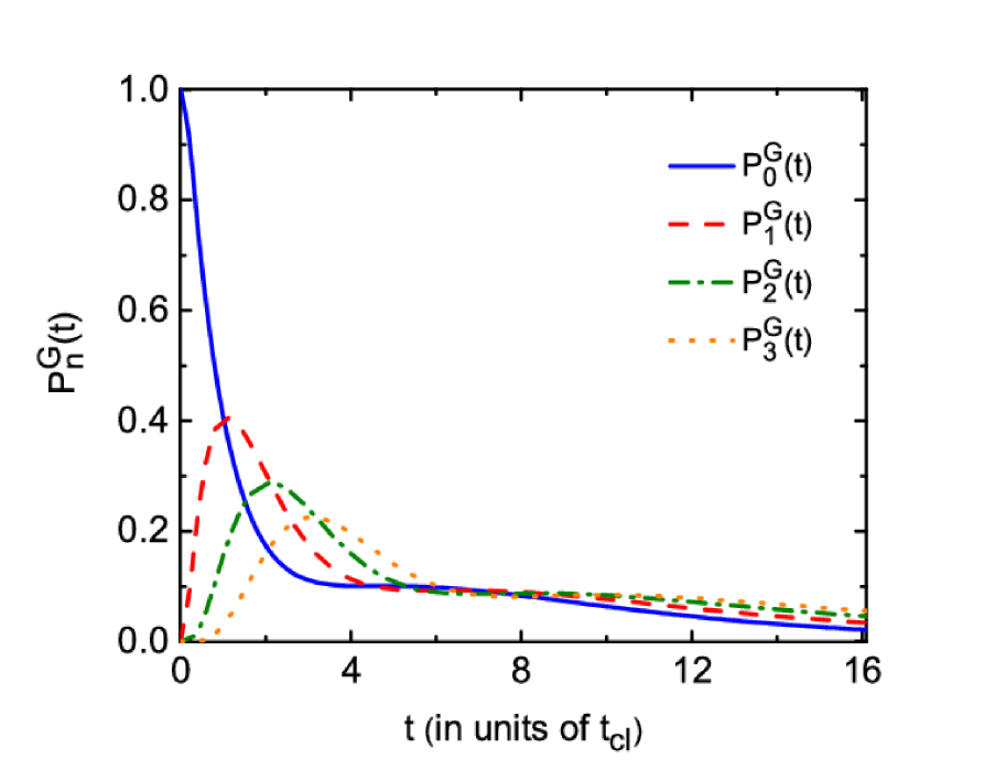
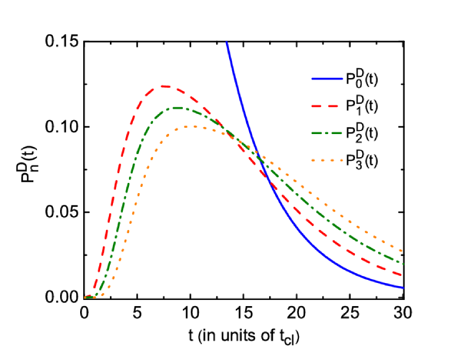
Figure 13: Probabilities to have $n$ clicks during the observation starting from the ground state ($P_{n}^{G}(t)$, left panel) or the dark state ($P_{n}^{D}(t)$, right panel) as functions of time. $\Omega_{D}=0.008$.

Now let us account for the periodicity of the braids. All strands in our case are defined on the interval $[k_{0},k_{0}+2\pi]$ with an arbitrary real $k_{0}$. It means that the starting and ending points in $k$ should be associated, so the braids are closed. These strands exist in three-dimensional space $\mathbb{R}^{3}$ formed by axes $k,Re[\lambda],Im[\lambda]$, and therefore the resulting closed braids are isotopic to links, which in turn form knots [76]. These links are oriented in our case, meaning that $\sigma_{i}\neq\sigma_{i}^{-1}$. This idea is illustrated in Fig. 12 for two strands, where we connect the starting and ending points of strands by dotted lines. The left diagram (braid word $\sigma_{1}^{2}$) forms two intersecting rings, this structure is known as the Hopf link. On the right diagram (braid word $\sigma_{1}$), moving along solid and dotted lines one arrives at the same point, so this structure effectively forms a single circle, known as unknot. By shrinking the dotted lines and continuously deforming the solid lines, we obtain diagrams similar to the ones shown on the right side of Fig. LABEL:fig:phases. Due to the arbitrary choice of $k_{0}$ and closed nature of the braids, the condition Eq. 48 is relaxed - although elements $\sigma_{1}$ and $\sigma_{2}$ are still non-commutative, braid words are now defined up to cyclic permutations. It means that if two braid words can be obtained one from the other by applying Eqs. 47, 49 and cyclic permutations, they belong to the same topological class. The braid index Eq. 13 counts the number of $\sigma_{i}$ elements in the braid word minus the number of $\sigma_{i}^{-1}$ elements, while other braid indexes introduced in Section IV count the number of braid elements (contributing with appropriate signs) encountered while moving along a particular closed path, similar to Fig. 12.

Appendix C Quantum jumps distribution

Here we analyze the time-dynamics of the quantum jumps distribution, in particular, the oscillating in time parity of the number of jump reported in Section V. As is evident from Fig. 4(a, b), the initial condition plays an important role for the dynamics of the system at short times ($\approx 3t_{cl}$), while afterwards this dynamics becomes universal. Hence, we start by considering probability to observe $n$ quantum jumps during the observation time $t$ either starting from the ground state or the dark state: $P^{G}_{n}(t)$, $P^{D}_{n}(t)$. For both cases we chose $\Omega_{D}=0.008$, corresponding to class IV, where $C(\pi,t)$ shows harmonic, sign-changing oscillations in time. These probability distributions can be analyzed the same way for other classes. We plot both distributions for $n=0,...,3$ in Fig. 13. Evidently, the jump probability distributions are non-Poissonian. By starting from the ground state (Fig. 13, left panel), one can observe distributions for $n$ jumps that initially look as Poissonian for the decay rate $\Gamma_{B}$ (note that each $P_{n}^{G}(t)$ peaks at $t_{n}=n\Gamma_{B}^{-1}$), but have an additional (very broad) peak in their long-time tails with very slow decay. We interpret this as follows - starting from the ground state, the system is most probably trapped within $G\rightleftharpoons B$ transitions, but has a small probability of escaping into the dark state. Such an event would drastically reduce the number of observed jumps. Moreover, if the system does not exhibit $\approx n$ jumps over time $n\Gamma_{B}^{-1}$, this indicates that the system has most probably escaped into the dark state and will likely stay there even longer (since $\Gamma_{D}\ll\Gamma_{B}$), further increasing the relative weights of small-$n$ observations over long times. This provides the timescale for the second maximum in the probability distributions, $t_{n}\simeq n\Gamma_{B}^{-1}+\Gamma_{D}^{-1}$. The situation is reversed when the system is initially prepared in the dark state (Fig. 13, right panel). In addition to the jump probabilities governed by the dark state decay rate, there is a chance that the system escapes into the bright sector, leading to a substantial shift of the jump probability distributions towards shorter times as compared to what one would except from the $\Gamma_{D}$ rate (the plotted distributions $P_{n}^{D}(t)$ have peaks at $t_{n}\approx n\Gamma_{B}^{-1}+\Gamma_{D}^{-1}$).
Next we analyze the oscillations of the “staggered” probability distribution $C(\pi,t)$. For that, we introduce the partial sum of the jump probabilities $P^{(N)}(t)$, which sums probabilities to observe from $0$ to $N$ quantum jumps during observation time $t$, weighted with signs according to their parities

$$P^{(N)}(t)=\sum_{l=0}^{N}(-1)^{l}P_{l}^{G}(t).$$ (50)

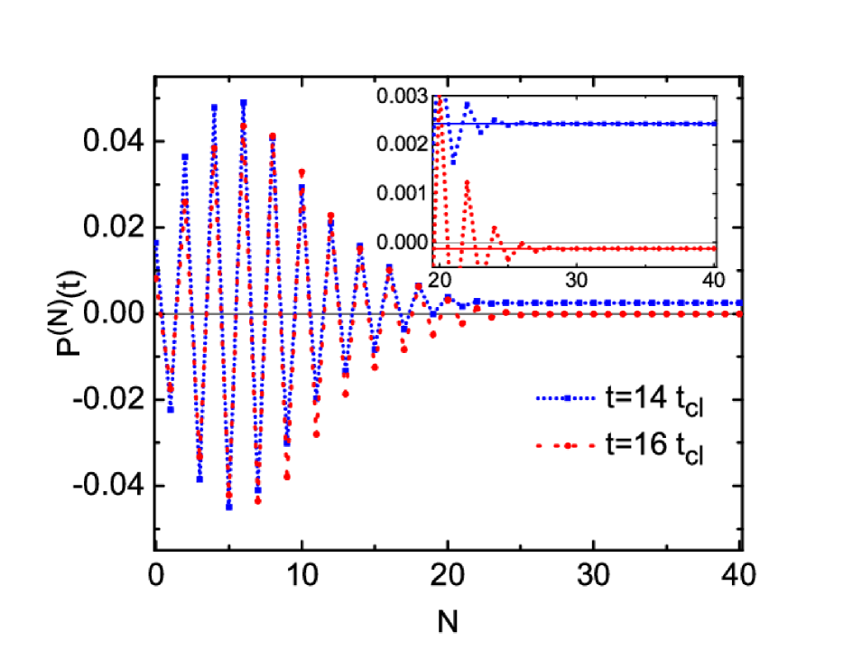
Figure 14: Partial sum $P^{(N)}(t)$ as a function of $N$ for $t=14t_{cl}$ (blue points) and $t=16t_{cl}$ (red points). $\Omega_{D}=0.01$. Inset: Late time saturation of the corresponding values to positive $C(\pi,14t_{cl})$ (blue line) and negative $C(\pi,16t_{cl})$ (red line).

For $N\rightarrow\infty$, this expression simply turns into $C(\pi,t)$, which is the Fourier transform of the jump probabilities taken at $k=\pi$:

$$\lim_{N\rightarrow\infty}P^{(N)}(t)=C(\pi,t).$$ (51)

Note that in Eq. 50 we chose probabilities for a system initially prepared in the ground state, though this choice between G and D states is arbitrary and simply accounts for the difference between Figs. 4(a, b).

The analysis of the partial sum $P^{(N)}(t)$ allows us to discern the main processes responsible for oscillations of $C(\pi,t)$ in class IV. Namely, one immediately can see if a certain number of jumps strongly dominates (e.g. if $n=0$ or $n=1$ is the most probable and defines the whole structure of the distribution), or if it’s rather a collective effect arising from interplay of multiple possible outcomes. As can be seen from Fig. 14, the latter scenario is correct - probabilities for many different $n$ sum up, so $P^{(N)}(t)$ is strongly oscillating before it saturates to $C(\pi,t)$. In Fig. 14 (we chose there $\Omega_{D}=0.01$ to make the transitions easily visible), it saturates at time $t=14t_{cl}$ to $C(\pi,14t_{cl})=0.0024$ (blue line) and at time $t=16t_{cl}$ to $C(\pi,16t_{cl})=-0.00012$ (red line), note that the amplitudes of the transient oscillations are much larger than the eventual saturation values. In both cases, approximately $N\approx 2t/t_{cl}$ jumps make important contributions. This is because probabilities with relatively small numbers of jumps still give substantial contributions even at long times (see large tails in Fig. 13). On the other hand it is very unlikely to observe numbers of jumps considerably exceeding those predicted by the Poissonian distribution with the largest (of two) rate $\Gamma_{B}$ (so probabilities for $n\gg t/t_{cl}$ are strongly suppressed).

Appendix D Perturbations of an exceptional point

Here we consider a general Hamiltonian of a two level system exhibiting an exceptional point. The presence of the exceptional point means that this Hamiltonian is non-diagonalizable, and (after a proper re-scaling) can be represented there in a Jordan form

$$H_{EP}=\begin{pmatrix}\alpha-\textit{i}\beta&1\\ 0&\alpha-\textit{i}\beta\end{pmatrix},$$ (52)

where $\alpha$ and $\beta$ are real and imaginary parts of the degenerate eigenvalue. At the EP there is no basis of eigenvectors, instead there exists the Jordan chain $\ket{\psi_{1}},\ket{\psi_{2}}$ such that

$$H_{EP}\ket{\psi_{1}}=(\alpha-\textit{i}\beta)\ket{\psi_{1}},$$

$$H_{EP}\ket{\psi_{2}}=(\alpha-\textit{i}\beta)\ket{\psi_{2}}+\ket{\psi_{1}}$$ . (53)

Using Eq. 53 and Eq. 25, we can construct the corresponding Jordan chain of the Lindbladian

$$L_{EP}=-\textit{i}\left\{H_{EP}\otimes\mathbb{1}-\mathbb{1}\otimes\left(H_{EP}^{\dagger}\right)^{T}\right\}\ ,$$ (54)

in which the quantum jumps have been omitted for now. Defining $\rho_{ij}\equiv\ket{\psi_{i}}\bra{\psi_{j}}$, we obtain

$$L_{EP}\left[\frac{1}{2}\left(\rho_{12}+\rho_{21}\right)\right]=-2\beta\left[\frac{1}{2}\left(\rho_{12}+\rho_{21}\right)\right],$$ (55)

$$L_{EP}\rho_{11}=-2\beta\rho_{11},$$ (56)

$$L_{EP}\left[\frac{1}{2\textit{i}}\left(\rho_{12}-\rho_{21}\right)\right]=-2\beta\left[\frac{1}{2\textit{i}}\left(\rho_{12}-\rho_{21}\right)\right]+\rho_{11},$$ (57)

$$L_{EP}\left[\frac{1}{2}\rho_{22}\right]=-2\beta\left[\frac{1}{2}\rho_{22}\right]+\frac{1}{2\textit{i}}\left(\rho_{12}-\rho_{21}\right).$$ (58)

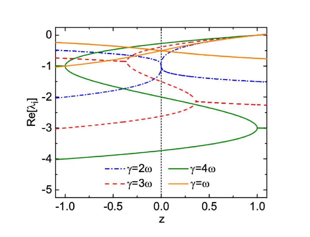
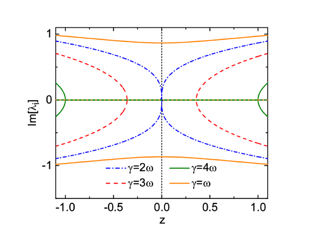
Figure 15: Exceptional point of the Lindbladian $L_{0}$ perturbed by the jump term $L_{J}$, Eq. 2 (numerical parameters are given in Eq. 63) with phase $k=0$ ($z>0$) and $k=\pi$ ($z<0$), $z=re^{\textit{i}k}$. Real (left panel) and imaginary (right panel) parts of the Lindbladian eigenvalues (in units of $\omega$) are plotted as functions of $z$ at fixed parameter $\gamma$. Blue dot-dashed line corresponds to the critical frequency where there is an exceptional point at $r=0$, while red dashed line, green solid line and orange solid line show the same system with changed parameter $\gamma$, they do not have an exceptional point at $r=0$, but the perturbed system acquires pairs of exceptional points at some values of the parameters $\gamma$ and $r$ (red and green lines) as the original third order exceptional point splits. Dashed black line is used as a guide for eyes and shows the case of absent quantum jumps.

As we see, the Jordan chain is formed by the following three vectors: $u_{1}=\rho_{11}$, $u_{2}=\frac{1}{2\textit{i}}(\rho_{12}-\rho_{21})$, $u_{3}=\frac{1}{2}\rho_{22}$, while the other eigenvector, $e=\frac{1}{2}(\rho_{12}+\rho_{21})$, does not participate in the EP, although its eigenvalue is degenerate with that of $u_{1}$.

The Jordan form of the Lindbladian $L_{EP}$ written in the basis $\{e,u_{1},u_{2},u_{3}\}$ takes the form

$$L_{EP}=\leavevmode\hbox to121.91pt{\vbox to74.13pt{\text{[drawing]}}}. -2\beta -2\beta -2\beta -2\beta \left(\vbox{\hrule height=34.6428pt,depth=34.6428pt,width=0.0pt}\right. \left.\vbox{\hrule height=34.6428pt,depth=34.6428pt,width=0.0pt}\right) -2\beta -2\beta -2\beta -2\beta \left(\vbox{\hrule height=34.6428pt,depth=34.6428pt,width=0.0pt}\right. \left.\vbox{\hrule height=34.6428pt,depth=34.6428pt,width=0.0pt}\right)$$ (59)

The dashed red box shows the Jordan form related to the third order EP. For simplicity, in what follows we consider only this reduced $3\times 3$ matrix. Next we consider a perturbed Liouvillian $L_{EP}+zL_{J}$, where, e.g., $L_{J}$ is the jump term, while $z\in\mathbb{C}$ is a perturbation parameter. A detailed analysis of perturbations in a vicinity of a third order EP can be found in [27, 80].

For the chain of right vectors $\{u_{1},u_{2},u_{3}\}$ one constructs the corresponding chain of vectors $\{v_{1},v_{2},v_{3}\}$, satisfying

$$v_{1}^{T}u_{1}=0,\,\,\,v_{1}^{T}u_{2}=0,\,\,\,v_{1}^{T}u_{3}=1$$

$$v_{3}^{T}u_{2}=0,\,\,\,v_{3}^{T}u_{3}=0,\,\,\,v_{2}^{T}u_{2}=1.$$ (60)

Note that the right vectors $\{u_{1},u_{2},u_{3}\}$ and the left vectors $\{v_{1}^{T},v_{2}^{T},v_{3}^{T}\}$ obey the self-orthogonality condition 60 rather than the one of the type of Eq. 15. Explicitly, we find

$$v_{1}=\begin{pmatrix}0\\ 0\\ 1\end{pmatrix},\,\,\,v_{2}=\begin{pmatrix}0\\ 1\\ 0\end{pmatrix},\,\,\,v_{3}=\begin{pmatrix}1\\ 0\\ 0\end{pmatrix}.$$ (61)

In general, the EP is lifted for the perturbed matrix $L_{EP}+zL_{J}$. The perturbed eigenvalues $\lambda^{(m)}$ are given in terms of the Puiseux series. For a small perturbation $|z|\ll 1$, they can be approximated as

$$\lambda^{(m)}=\lambda_{0}+\lambda_{1}^{(m)}r^{\frac{1}{3}}+o(r^{\frac{1}{3}}),$$ (62)

where $\lambda_{0}$ is the unperturbed degenerate eigenvalue at the exceptional point, $z=re^{\textit{i}k}$ is the perturbation parameter of Eq. 24, while $\lambda_{1}^{(m)}$ are the three complex roots of the equation $(\lambda_{1})^{3}=e^{\textit{i}k}v_{1}^{T}L_{J}u_{1}$. Note that $e^{\textit{i}k}v_{1}^{T}L_{J}u_{1}$ is real for $k=0$, thus one of the solutions has a positive real part, while two other have identical negative real parts. Thus even an infinitesimal positive $z$ immediately opens the Liouvillian gap, i.e., the longest living solution with the positive real part of $\lambda_{1}$ can no longer participate in any EP. Although, strictly speaking, this analysis is applied to $|z|\ll 1$, its interpolation up to $z=1$ is aligned with the results of [50] and restores the results of [38]. Interestingly, the structure of the perturbed eigenstates reverses at $k=\pi$, namely, the two longest lived eigenstates have the same real part and further form a second order EP.

Let us see how these general features appear in a particular example given by Eq. 26. Its effective Hamiltonian has an EP at $\gamma=2\omega$. Measuring all energies in units of $\omega$, we obtain the Jordan form of the EP Liouvillian $L_{EP}$ and the jump operator $L_{J}$

$$L_{EP}=\begin{pmatrix}-1&0&0&0\\ 0&-1&1&0\\ 0&0&-1&1\\ 0&0&0&-1\end{pmatrix},\,\,\,L_{J}=\begin{pmatrix}0&0&0&0\\ 0&0&0&0\\ 0&0&0&0\\ 0&1&0&0\end{pmatrix}.$$ (63)

The perturbed eigenvalues of Eq. 62 are constructed with

$$\lambda_{0}=-1,\,\,\,\lambda_{1}^{(n)}=e^{\textit{i}(k+2\pi n)/3}.$$ (64)

This gives the perturbed eigenvalues

$$k=0:\,\lambda^{(3)}=-1+r^{\frac{1}{3}},\,\lambda^{(1,2)}=-1+e^{\pm\textit{i}\frac{2\pi}{3}}r^{\frac{1}{3}};$$ (65)

$$k=\pi:\,\lambda^{(3,2)}=-1+e^{\pm\textit{i}\frac{\pi}{3}}r^{\frac{1}{3}},\,\lambda^{(1)}=-1-r^{\frac{1}{3}}.$$ (66)

Due to simplicity of the perturbation term in Eq. 63, these results turn out to be exact, even for $r=1$. The numerical results showing the effects of quantum jumps and the duality between $k=0$ and $k=\pi$ are shown in Fig. 8. As expected, one of the eigenvalues is not involved in the formation of the EP and is not affected by its perturbation.

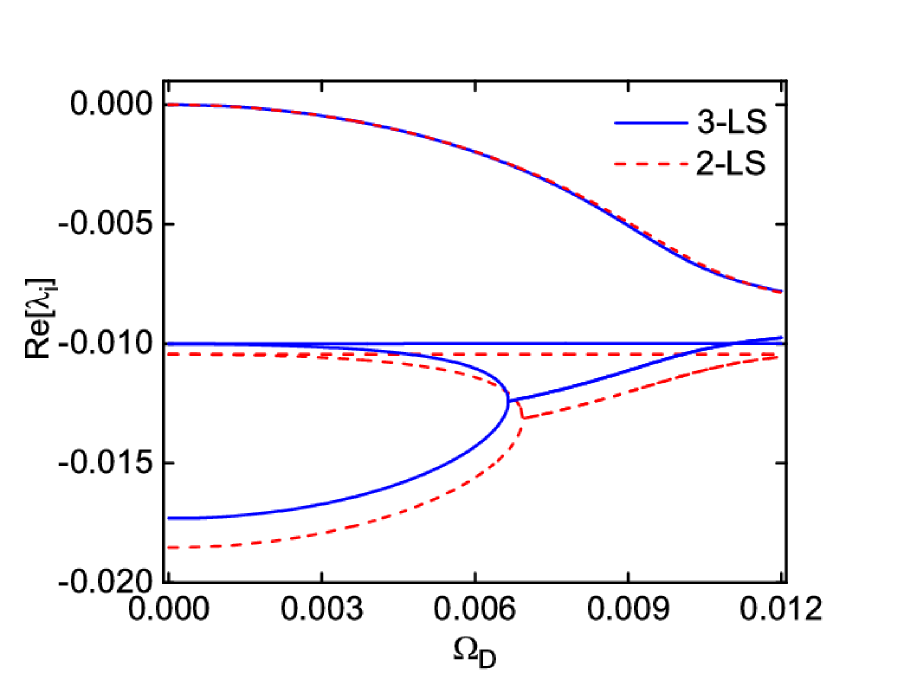
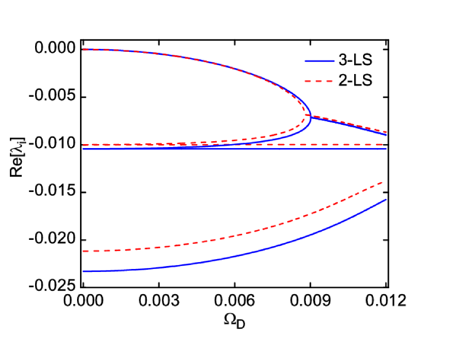
Figure 16: Eigenvalues (real parts) $\lambda_{i}$ of the three level system Lindbladian Eq. 5 with the jump term suppressed by $z=\pm 0.1$ (blue solid lines, 3-LS) and eigenvalues of the effective Ground-Dark two level system’s Lindbladian obtained via adiabatic elimination (red dashed line, 2-LS) as functions of the driving frequency $\Omega_{D}$. Left panel: $z=0.1$, right panel: $z=-0.1$. For the three level system, only four relevant eigenvalues (long-living states forming an exceptional point) are plotted. The reduced system retains an exceptional point of the same structure in close proximity to the original exceptional point.

Furthermore, the eigenvalues of $L_{EP}+zL_{J}$ in Eq. 26 allow for analytical solutions for arbitrary parameters. After rescaling the eigenvalues in units of $\omega$, there is one $z$-independent eigenvalue, which does not participate in the EP and three others are given by roots of the third order polynomial,

$$\lambda^{(1)}=\frac{1}{2}x_{1},\,\lambda^{(2)}=\frac{1}{2}x_{2},\,\lambda^{(3)}=\frac{1}{2}x_{3},\,\lambda^{(4)}=-\frac{1}{2}\gamma,$$ (67)

where $x_{1,2,3}$ are roots of the polynomial

$$x^{3}+3\gamma x^{2}+(4+2\gamma^{2})x+4\gamma(1-z)=0.$$ (68)

The real parts of the eigenvalues $\lambda^{(i)}$ for fixed $z$ are plotted in Fig. 8 as functions of $\gamma$. Additionally, we plot real and imaginary parts of these exact solutions in Fig. 15 for various fixed $\gamma$ as functions of (real) $z$. It is evident from this plot that a change from $k=0$ to $k=\pi$ flips the structure of the eigenvalues simply due to the symmetry of the roots of a cubic equation. Moreover, the EP that appears without quantum jumps at some critical value of $\gamma$ shifts for non-zero $z$ but survives, though at different $\gamma$. E.g. in Fig. 15 there are EPs at $\gamma=2\omega$ for $z=0$ (dot dashed blue line), at $\gamma=3\omega$ for $z=\pm 0.5$ (dashed red line), and at $\gamma=4$ for $z=\pm 1$ (solid green line).
It’s worth mentioning that a special case $v_{1}^{T}L_{J}u_{1}=0$ is in principle possible. Then Eq. 62 is no longer applicable and the EP is perturbed by a linear term and a pair of square root terms [27, 80]. This situation is unlikely for realistic quantum jump models in two-level-systems, but even in this case the phase $k=\pi$ flips the order of the perturbed eigenstates with respect to $k=0$, making a formation of an EP between two least decaying states possible.

Appendix E Adiabatic elimination

When a system consists of two coupled subsystems with asymptotically stable hierarchy of characteristic times – one subsystem exhibits slow dynamics and the other has fast dynamics – there is a method for systematic elimination of the fast subsystem and for arriving at an effective description of the reduced slow subsystem. This method is known as adiabatic elimination. Most generally, it applies at the Lindbladian level such that the reduced density matrix of the subsystem is governed by a new effective Lindbladian [84]. If the dynamics of the whole system can be described in terms of a non-Hermitian Hamiltonian, then an effective description of the reduced system has also the Hamiltonian form [83].
In the following, we do not go into details on a formal and rigorous description of this procedure in terms of the projection operators and construction of the perturbation theory in terms of these operators (for details see [84, 85, 86, 87]), but rather describe the exact (in the sense of perturbation theory) numerical approach to the adiabatic elimination, which can be easily implemented for small systems ([81, 82, 83]).
Let’s consider the Lindbladian dynamics of our three-level system $\{G,\,D,\,B\}$. We write its density matrix $\rho$ in the vector form, $\dot{\rho}(t)=\mathcal{L}\rho$, where $\mathcal{L}$ is the system’s Lindbladian superoperator. Then we reorder the column representing the density matrix as well as the Lindbladian as follows

$$\rho=\begin{pmatrix}\rho_{S}\\ \rho_{F}\end{pmatrix},\,\,\,\mathcal{L}=\begin{pmatrix}\mathbf{S}&\mathbf{C}\\ \mathbf{C}^{T}&\mathbf{F}\end{pmatrix}.$$ (69)

Here $\rho_{S}$ is a column of four elements comprising the slow system: populations of D and G states and coherences between them (namely, $\rho_{GG}$, $\rho_{GD}$, $\rho_{DG}$, $\rho_{DD}$), $\rho_{F}$ is a column of five elements with fast dynamics, which involve $B$ state and transitions to/from it. $\mathbf{S}$ and $\mathbf{F}$ are $4\times 4$ and $5\times 5$ matrices describing Lindbladian dynamics of the slow and fast sectors correspondingly. $\mathbf{C}$ and $\mathbf{C}^{T}$ are matrices describing transitions between these sectors. The essential idea behind the adiabatic elimination is that due to the large separation of time scales the fast system provides a constant background for the slow system’s evolution. Hence, the $\rho_{F}$ elements can be considered constant in time. In our case, this assumption is justified by a clear hierarchy of transition rates $\gamma_{B}\gg\Gamma_{B}\gg\Gamma_{D}$,

$$\begin{pmatrix}\dot{\rho}_{S}(t)\\ \dot{\rho}_{F}(t)\end{pmatrix}\simeq\begin{pmatrix}\dot{\rho}_{S}(t)\\ 0\end{pmatrix}=\begin{pmatrix}\mathbf{S}&\mathbf{C}\\ \mathbf{C}^{T}&\mathbf{F}\end{pmatrix}\begin{pmatrix}\rho_{S}(t)\\ \rho_{F}(t)\end{pmatrix}.$$ (70)

This brings us to

$$\dot{\rho_{S}}=\mathcal{L}_{eff}\rho_{S}=\left(\mathbf{S}-\mathbf{C}\mathbf{F}^{-1}\mathbf{C}^{T}\right)\rho_{S}.$$ (71)

This reduced effective Lindbladian describes the dynamics of the slow subsystem. For the numerical implementation of a similar procedure in an arbitrary large system see [55] (with the difference that the reduction is done there to describe only populations of a full system, rather than populations and coherences of a subsystem). The same procedure can be straightforwardly implemented on the Schrödinger equation level in the absence of quantum jumps (e.g. see [41] for the Hamiltonian adiabatic elimination in the three level system). We compare the reduced effective two level system Hamiltonian with the full three level system Hamiltonian in Fig. 9. Evidently, the two most important states are almost not affected by this procedure at all - they preserve the EP with only a minor shift in frequency $\Omega_{D}$. The same applies to the Lindbladian dynamics. As demonstrated in Fig. 16, for the Lindbladian with reduced weight of quantum jumps ($|z|=0.1$), the three longest living states preserve their structures both for $k=0$ and $k=\pi$. Additionally, we see that the adiabatic elimination is most accurate for the state with the smallest real part, regardless if it contains an EP. Further eigenstates are approximated less accurately due to increase of their decay, though they still preserve the EP structure.

References

- Moiseyev [2011] N. Moiseyev, Non-Hermitian Quantum Mechanics (Cambridge University Press, New York, 2011).
- Uzdin et al. [2011] R. Uzdin, A. Mailybaev, and N. Moiseyev, On the observability and asymmetry of adiabatic state flips generated by exceptional points, Journal of Physics A: Mathematical and Theoretical 44, 435302 (2011).
- Heiss [2012] W. D. Heiss, The physics of exceptional points, Journal of Physics A: Mathematical and Theoretical 45, 444016 (2012).
- Ashida et al. [2020] Y. Ashida, Z. Gong, and M. Ueda, Non-Hermitian physics, Advances in Physics 69, 249–435 (2020).
- Berry and Uzdin [2011] M. V. Berry and R. Uzdin, Slow non-Hermitian cycling: exact solutions and the Stokes phenomenon, Journal of Physics A: Mathematical and Theoretical 44, 435303 (2011).
- El-Ganainy et al. [2018] R. El-Ganainy, K. G. Makris, M. Khajavikhan, Z. H. Musslimani, S. Rotter, and D. N. Christodoulides, Non-Hermitian physics and symmetry, Nature Physics 14, 11–19 (2018).
- Guria et al. [2024] C. Guria, Q. Zhong, S. K. Ozdemir, Y. S. S. Patil, R. El-Ganainy, and J. G. E. Harris, Resolving the topology of encircling multiple exceptional points, Nature Communications 15, 1369 (2024).
- Álvarez et al. [2006] G. A. Álvarez, E. P. Danieli, P. R. Levstein, and H. M. Pastawski, Environmentally induced quantum dynamical phase transition in the spin swapping operation, The Journal of Chemical Physics 124, 194507 (2006).
- Pastawski [2007] H. M. Pastawski, Revisiting the Fermi Golden Rule: Quantum dynamical phase transition as a paradigm shift, Physica B: Condensed Matter 398, 278–286 (2007).
- Heyl et al. [2013] M. Heyl, A. Polkovnikov, and S. Kehrein, Dynamical quantum phase transitions in the transverse-field ising model, Phys. Rev. Lett. 110, 135704 (2013).
- Eleuch and Rotter [2013] H. Eleuch and I. Rotter, Width bifurcation and dynamical phase transitions in open quantum systems, Phys. Rev. E 87, 052136 (2013).
- Eleuch and Rotter [2016] H. Eleuch and I. Rotter, Clustering of exceptional points and dynamical phase transitions, Phys. Rev. A 93, 042116 (2016).
- Deng et al. [2023] K. Deng, X. Li, and B. Flebus, Exceptional points as signatures of dynamical magnetic phase transitions, Phys. Rev. B 107, L100402 (2023).
- Kumar et al. [2020] P. Kumar, A. Romito, and K. Snizhko, Quantum Zeno effect with partial measurement and noisy dynamics, Phys. Rev. Res. 2, 043420 (2020).
- Fröml et al. [2020] H. Fröml, C. Muckel, C. Kollath, A. Chiocchetta, and S. Diehl, Ultracold quantum wires with localized losses: Many-body quantum Zeno effect, Phys. Rev. B 101, 144301 (2020).
- Mouloudakis and Lambropoulos [2022] G. Mouloudakis and P. Lambropoulos, Coalescence of non-Markovian dissipation, quantum Zeno effect, and non-Hermitian physics in a simple realistic quantum system, Phys. Rev. A 106, 053709 (2022).
- Dubey et al. [2023] V. Dubey, R. Chetrite, and A. Dhar, Quantum resetting in continuous measurement induced dynamics of a qubit, Journal of Physics A: Mathematical and Theoretical 56, 154001 (2023).
- Makris et al. [2008] K. G. Makris, R. El-Ganainy, D. N. Christodoulides, and Z. H. Musslimani, Beam dynamics in symmetric optical lattices, Phys. Rev. Lett. 100, 103904 (2008).
- Bittner et al. [2012] S. Bittner, B. Dietz, U. Günther, H. L. Harney, M. Miski-Oglu, A. Richter, and F. Schäfer, symmetry and spontaneous symmetry breaking in a microwave billiard, Phys. Rev. Lett. 108, 024101 (2012).
- Minganti et al. [2018] F. Minganti, A. Biella, N. Bartolo, and C. Ciuti, Spectral theory of Liouvillians for dissipative phase transitions, Phys. Rev. A 98, 042118 (2018).
- Gong et al. [2018] Z. Gong, Y. Ashida, K. Kawabata, K. Takasan, S. Higashikawa, and M. Ueda, Topological phases of non-Hermitian systems, Phys. Rev. X 8, 031079 (2018).
- Lieu [2018] S. Lieu, Topological symmetry classes for non-Hermitian models and connections to the bosonic Bogoliubov–de Gennes equation, Phys. Rev. B 98, 115135 (2018).
- Martinez Alvarez et al. [2018a] V. M. Martinez Alvarez, J. E. Barrios Vargas, and L. E. F. Foa Torres, Non-Hermitian robust edge states in one dimension: Anomalous localization and eigenspace condensation at exceptional points, Phys. Rev. B 97, 121401 (2018a).
- Martinez Alvarez et al. [2018b] V. M. Martinez Alvarez, J. E. Barrios Vargas, M. Berdakin, and L. E. F. Foa Torres, Topological states of non-Hermitian systems, The European Physical Journal Special Topics 227, 1295–1308 (2018b).
- Foa Torres [2019] L. E. F. Foa Torres, Perspective on topological states of non-Hermitian lattices, Journal of Physics: Materials 3, 014002 (2019).
- Kawabata et al. [2019] K. Kawabata, T. Bessho, and M. Sato, Classification of exceptional points and non-Hermitian topological semimetals, Phys. Rev. Lett. 123, 066405 (2019).
- Seyranian and Mailybaev [2003] A. P. Seyranian and A. A. Mailybaev, Multiparameter Stability Theory with Mechanical Applications (World Scientific, Singapore, 2003).
- Znojil [2022] M. Znojil, Confluences of exceptional points and a systematic classification of quantum catastrophes, Scientific Reports 12, 3355 (2022).
- Hu et al. [2023] J. Hu, R.-Y. Zhang, Y. Wang, X. Ouyang, Y. Zhu, H. Jia, and C. T. Chan, Non-Hermitian swallowtail catastrophe revealing transitions among diverse topological singularities, Nature Physics 19, 1098–1103 (2023).
- Bansil et al. [2016] A. Bansil, H. Lin, and T. Das, Colloquium: Topological band theory, Rev. Mod. Phys. 88, 021004 (2016).
- Wojcik et al. [2020] C. C. Wojcik, X.-Q. Sun, T. Bzdušek, and S. Fan, Homotopy characterization of non-Hermitian Hamiltonians, Phys. Rev. B 101, 205417 (2020).
- Chen et al. [2017] W. Chen, Ş. K. Özdemir, G. Zhao, J. Wiersig, and L. Yang, Exceptional points enhance sensing in an optical microcavity, Nature 548, 192–196 (2017).
- Hodaei et al. [2017] H. Hodaei, A. U. Hassan, S. Wittek, H. Garcia-Gracia, R. El-Ganainy, D. N. Christodoulides, and M. Khajavikhan, Enhanced sensitivity at higher-order exceptional points, Nature 548, 187–191 (2017).
- Metelmann and Clerk [2015] A. Metelmann and A. A. Clerk, Nonreciprocal photon transmission and amplification via reservoir engineering, Phys. Rev. X 5, 021025 (2015).
- Zhong et al. [2020] Q. Zhong, S. K. Ozdemir, A. Eisfeld, A. Metelmann, and R. El-Ganainy, Exceptional-point-based optical amplifiers, Phys. Rev. Appl. 13, 014070 (2020).
- Kumar et al. [2022] P. Kumar, K. Snizhko, Y. Gefen, and B. Rosenow, Optimized steering: Quantum state engineering and exceptional points, Phys. Rev. A 105, L010203 (2022).
- Li et al. [2023] Z.-Z. Li, W. Chen, M. Abbasi, K. W. Murch, and K. B. Whaley, Speeding up entanglement generation by proximity to higher-order exceptional points, Phys. Rev. Lett. 131, 100202 (2023).
- Minganti et al. [2019] F. Minganti, A. Miranowicz, R. W. Chhajlany, and F. Nori, Quantum exceptional points of non-Hermitian Hamiltonians and Liouvillians: The effects of quantum jumps, Phys. Rev. A 100, 062131 (2019).
- Chen et al. [2022] W. Chen, M. Abbasi, B. Ha, S. Erdamar, Y. N. Joglekar, and K. W. Murch, Decoherence-induced exceptional points in a dissipative superconducting qubit, Phys. Rev. Lett. 128, 110402 (2022).
- Naghiloo et al. [2019] M. Naghiloo, M. Abbasi, Y. N. Joglekar, and K. W. Murch, Quantum state tomography across the exceptional point in a single dissipative qubit, Nature Physics 15, 1232–1236 (2019).
- Minev et al. [2019] Z. K. Minev, S. O. Mundhada, S. Shankar, P. Reinhold, R. Gutiérrez-Jáuregui, R. J. Schoelkopf, M. Mirrahimi, H. J. Carmichael, and M. H. Devoret, To catch and reverse a quantum jump mid-flight, Nature 570, 200–204 (2019).
- Chen et al. [2021] W. Chen, M. Abbasi, Y. N. Joglekar, and K. W. Murch, Quantum jumps in the non-Hermitian dynamics of a superconducting qubit, Phys. Rev. Lett. 127, 140504 (2021).
- Levitov and Lesovik [1993] L. S. Levitov and G. B. Lesovik, Charge distribution in quantum shot noise, JETP Lett. 58, 230 (1993).
- Levitov et al. [1996] L. S. Levitov, H. Lee, and G. B. Lesovik, Electron counting statistics and coherent states of electric current, Journal of Mathematical Physics 37, 4845 (1996).
- Nazarov and Kindermann [2003] Y. V. Nazarov and M. Kindermann, Full counting statistics of a general quantum mechanical variable, The European Physical Journal B - Condensed Matter 35, 413–420 (2003).
- Flindt et al. [2008] C. Flindt, T. Novotný, A. Braggio, M. Sassetti, and A.-P. Jauho, Counting statistics of non-Markovian quantum stochastic processes, Phys. Rev. Lett. 100, 150601 (2008).
- Li et al. [2014] F. Li, J. Ren, and N. A. Sinitsyn, Quantum Zeno effect as a topological phase transition in full counting statistics and spin noise spectroscopy, EPL (Europhysics Letters) 105, 27001 (2014).
- Riwar [2019] R.-P. Riwar, Fractional charges in conventional sequential electron tunneling, Phys. Rev. B 100, 245416 (2019).
- Kleinherbers et al. [2023] E. Kleinherbers, A. Schünemann, and J. König, Full counting statistics in a Majorana single-charge transistor, Phys. Rev. B 107, 195407 (2023).
- Minganti et al. [2020] F. Minganti, A. Miranowicz, R. W. Chhajlany, I. I. Arkhipov, and F. Nori, Hybrid-Liouvillian formalism connecting exceptional points of non-Hermitian Hamiltonians and Liouvillians via postselection of quantum trajectories, Phys. Rev. A 101, 062112 (2020).
- Vijay et al. [2011] R. Vijay, D. H. Slichter, and I. Siddiqi, Observation of quantum jumps in a superconducting artificial atom, Phys. Rev. Lett. 106, 110502 (2011).
- Vool et al. [2014] U. Vool, I. M. Pop, K. Sliwa, B. Abdo, C. Wang, T. Brecht, Y. Y. Gao, S. Shankar, M. Hatridge, G. Catelani, M. Mirrahimi, L. Frunzio, R. J. Schoelkopf, L. I. Glazman, and M. H. Devoret, Non-Poissonian quantum jumps of a fluxonium qubit due to quasiparticle excitations, Phys. Rev. Lett. 113, 247001 (2014).
- Slichter et al. [2016] D. H. Slichter, C. Müller, R. Vijay, S. J. Weber, A. Blais, and I. Siddiqi, Quantum Zeno effect in the strong measurement regime of circuit quantum electrodynamics, New Journal of Physics 18, 053031 (2016).
- Spiecker et al. [2023] M. Spiecker, P. Paluch, N. Gosling, N. Drucker, S. Matityahu, D. Gusenkova, S. Günzler, D. Rieger, I. Takmakov, F. Valenti, P. Winkel, R. Gebauer, O. Sander, G. Catelani, A. Shnirman, A. V. Ustinov, W. Wernsdorfer, Y. Cohen, and I. M. Pop, Two-level system hyperpolarization using a quantum Szilard engine, Nature Physics 19, 1320–1325 (2023).
- Spiecker et al. [2024] M. Spiecker, A. I. Pavlov, A. Shnirman, and I. M. Pop, Solomon equations for qubit and two-level systems: Insights into non-Poissonian quantum jumps, Phys. Rev. A 109, 052218 (2024).
- Campagne-Ibarcq et al. [2014] P. Campagne-Ibarcq, L. Bretheau, E. Flurin, A. Auffèves, F. Mallet, and B. Huard, Observing interferences between past and future quantum states in resonance fluorescence, Phys. Rev. Lett. 112, 180402 (2014).
- Naghiloo et al. [2016] M. Naghiloo, N. Foroozani, D. Tan, A. Jadbabaie, and K. W. Murch, Mapping quantum state dynamics in spontaneous emission, Nature Communications 7, 11527 (2016).
- Naghiloo et al. [2017] M. Naghiloo, D. Tan, P. M. Harrington, P. Lewalle, A. N. Jordan, and K. W. Murch, Quantum caustics in resonance-fluorescence trajectories, Phys. Rev. A 96, 053807 (2017).
- Cook and Kimble [1985] R. J. Cook and H. J. Kimble, Possibility of direct observation of quantum jumps, Phys. Rev. Lett. 54, 1023 (1985).
- Nagourney et al. [1986] W. Nagourney, J. Sandberg, and H. Dehmelt, Shelved optical electron amplifier: Observation of quantum jumps, Phys. Rev. Lett. 56, 2797 (1986).
- Sauter et al. [1986] T. Sauter, W. Neuhauser, R. Blatt, and P. E. Toschek, Observation of quantum jumps, Phys. Rev. Lett. 57, 1696 (1986).
- Bergquist et al. [1986] J. C. Bergquist, R. G. Hulet, W. M. Itano, and D. J. Wineland, Observation of quantum jumps in a single atom, Phys. Rev. Lett. 57, 1699 (1986).
- Garrahan and Lesanovsky [2010] J. P. Garrahan and I. Lesanovsky, Thermodynamics of quantum jump trajectories, Phys. Rev. Lett. 104, 160601 (2010).
- Lesanovsky et al. [2013] I. Lesanovsky, M. van Horssen, M. Guţă, and J. P. Garrahan, Characterization of dynamical phase transitions in quantum jump trajectories beyond the properties of the stationary state, Phys. Rev. Lett. 110, 150401 (2013).
- Garrahan and Guţă [2018] J. P. Garrahan and M. Guţă, Catching and reversing quantum jumps and thermodynamics of quantum trajectories, Phys. Rev. A 98, 052137 (2018).
- Perfetto et al. [2022] G. Perfetto, F. Carollo, and I. Lesanovsky, Thermodynamics of quantum-jump trajectories of open quantum systems subject to stochastic resetting, SciPost Phys. 13, 079 (2022).
- Schaller [2014] G. Schaller, Open Quantum Systems Far from Equilibrium (Springer International Publishing, Cham, Switzerland, 2014).
- Wang et al. [2021] K. Wang, A. Dutt, C. C. Wojcik, and S. Fan, Topological complex-energy braiding of non-Hermitian bands, Nature 598, 59–64 (2021).
- Zhang et al. [2023a] Q. Zhang, L. Zhao, X. Liu, X. Feng, L. Xiong, W. Wu, and C. Qiu, Experimental characterization of three-band braid relations in non-Hermitian acoustic lattices, Phys. Rev. Res. 5, L022050 (2023a).
- Zhang et al. [2023b] Q. Zhang, Y. Li, H. Sun, X. Liu, L. Zhao, X. Feng, X. Fan, and C. Qiu, Observation of acoustic non-Hermitian Bloch braids and associated topological phase transitions, Phys. Rev. Lett. 130, 017201 (2023b).
- König et al. [2023] J. L. K. König, K. Yang, J. C. Budich, and E. J. Bergholtz, Braid-protected topological band structures with unpaired exceptional points, Phys. Rev. Res. 5, L042010 (2023).
- Ren and Sinitsyn [2013] J. Ren and N. A. Sinitsyn, Braid group and topological phase transitions in nonequilibrium stochastic dynamics, Phys. Rev. E 87, 050101 (2013).
- Ivanov and Abanov [2010] D. A. Ivanov and A. G. Abanov, Phase transitions in full counting statistics for periodic pumping, EPL (Europhysics Letters) 92, 37008 (2010).
- Hu and Zhao [2021] H. Hu and E. Zhao, Knots and non-Hermitian Bloch bands, Phys. Rev. Lett. 126, 010401 (2021).
- Patil et al. [2022] Y. S. S. Patil, J. Höller, P. A. Henry, C. Guria, Y. Zhang, L. Jiang, N. Kralj, N. Read, and J. G. E. Harris, Measuring the knot of non-Hermitian degeneracies and non-commuting braids, Nature 607, 271–275 (2022).
- Kassel and Turaev [2008] C. Kassel and V. Turaev, Braid Groups (Springer, New York, 2008).
- Birman and Menasco [2008] J. S. Birman and W. W. Menasco, A note on closed 3-braids, Communications in Contemporary Mathematics 10, 1033–1047 (2008).
- Aldrovandi and Rocha Jr. [2021] R. Aldrovandi and R. d. Rocha Jr., A Gentle Introduction to Knots, Links and Braids (World Scientific, Singapore, 2021).
- Heiss [2008] W. D. Heiss, Chirality of wavefunctions for three coalescing levels, Journal of Physics A: Mathematical and Theoretical 41, 244010 (2008).
- Demange and Graefe [2011] G. Demange and E.-M. Graefe, Signatures of three coalescing eigenfunctions, Journal of Physics A: Mathematical and Theoretical 45, 025303 (2011).
- Shnirman and Schön [1998] A. Shnirman and G. Schön, Quantum measurements performed with a single-electron transistor, Phys. Rev. B 57, 15400 (1998).
- Makhlin et al. [2000] Y. Makhlin, G. Schön, and A. Shnirman, Statistics and noise in a quantum measurement process, Phys. Rev. Lett. 85, 4578 (2000).
- Brion et al. [2007] E. Brion, L. H. Pedersen, and K. Mølmer, Adiabatic elimination in a lambda system, Journal of Physics A: Mathematical and Theoretical 40, 1033–1043 (2007).
- Mirrahimi and Rouchon [2009] M. Mirrahimi and P. Rouchon, Singular perturbations and Lindblad-Kossakowski differential equations, IEEE Transactions on Automatic Control 54, 1325–1329 (2009).
- Reiter and Sørensen [2012] F. Reiter and A. S. Sørensen, Effective operator formalism for open quantum systems, Phys. Rev. A 85, 032111 (2012).
- Azouit et al. [2017] R. Azouit, F. Chittaro, A. Sarlette, and P. Rouchon, Towards generic adiabatic elimination for bipartite open quantum systems, Quantum Science and Technology 2, 044011 (2017).
- Finkelstein-Shapiro et al. [2020] D. Finkelstein-Shapiro, D. Viennot, I. Saideh, T. Hansen, T. Pullerits, and A. Keller, Adiabatic elimination and subspace evolution of open quantum systems, Phys. Rev. A 101, 042102 (2020).
- Snizhko et al. [2020] K. Snizhko, P. Kumar, and A. Romito, Quantum zeno effect appears in stages, Phys. Rev. Res. 2, 033512 (2020).
- Pöpperl et al. [2024] P. Pöpperl, I. V. Gornyi, D. B. Saakian, and O. M. Yevtushenko, Localization, fractality, and ergodicity in a monitored qubit, Phys. Rev. Res. 6, 013313 (2024).
- Fowler et al. [2012] A. G. Fowler, M. Mariantoni, J. M. Martinis, and A. N. Cleland, Surface codes: Towards practical large-scale quantum computation, Phys. Rev. A 86, 032324 (2012).
- Caruso et al. [2014] F. Caruso, V. Giovannetti, C. Lupo, and S. Mancini, Quantum channels and memory effects, Rev. Mod. Phys. 86, 1203 (2014).
- Martinis [2015] J. M. Martinis, Qubit metrology for building a fault-tolerant quantum computer, npj Quantum Information 1, 15005 (2015).