Projection-to-Born-improved Subtractions at NNLO

Abstract

While the current frontier in fixed-order precision for collider observables is N³LO, important steps are necessary to consolidate NNLO cross-section predictions with improved stability and efficiency. Slicing methods have been successfully applied to obtain NNLO and N³LO predictions, but have shown poor performance in the presence of fiducial cuts due to large kinematical power corrections. In this paper we implement Projection-to-Born-improved $q_{T}$ (P2B $q_{T}$) and jettiness (P2B $\tau_{0}$) subtractions for a large class of color singlet processes in MCFM. This method allows for the efficient evaluation of fiducial power corrections in any non-local subtraction scheme using a Projection-to-Born subtraction. We demonstrate the significant numerical improvements of this method based on fiducial Drell-Yan and Higgs cross-sections. Moreover, with fiducial power corrections removed via this method, the leading-logarithmic power corrections that have only been calculated without fiducial cuts can be included, further improving the calculations. For di-photon production with photon isolation, we devise a novel method in combination with P2B-improved subtractions, which we name $\text{P2B}{}_{\gamma}$ $\tau_{0}$, and $\text{P2B}{}_{\gamma}~{}q_{T}$ for the two subtraction schemes, respectively. This method allows the inclusion of both fiducial power corrections due to kinematic cuts on the photons and a set of isolation power corrections in the fragmentation channel where a quark may enter the isolation cone. We find significant improvements in the convergence of NNLO di-photon cross-sections with photon isolation cuts, demonstrating that it is possible to achieve a stable and efficient calculation of di-photon cross-sections using slicing methods.

1 Introduction

The Large Hadron Collider (LHC) has been instrumental in advancing our understanding of fundamental physics, largely due to its capability to measure Standard Model (SM) processes with unprecedented precision. LHC measurements of key benchmark processes, such as the production of electroweak bosons ($W^{\pm}$, $Z$), have reached an astonishing level of accuracy, previously only limited by the luminosity uncertainty CMS:2021xjt ; ATLAS:2022hro , see for example refs. ATLAS:2024nrd ; CMS:2019raw ; ATLAS:2019zci . Such a level of precision has not yet been reached for Higgs boson measurements since the main source of experimental uncertainty comes from the limited statistical power of current data sets ATLAS:2022fnp ; ATLAS:2022qef ; CMS:2023gjz ; ATLAS:2023tnc . However, the situation will be dramatically different for a projected seven-fold increase of statistics at the High Luminosity LHC (HL-LHC) ATLAS:2019mfr ; ATLAS:2022hsp .

In order to match the accuracy of data from the LHC, precise theoretical predictions for Standard Model scattering processes are required. To this end, one must include radiative corrections from quantum chromodynamics (QCD) at least to the next-to-next-to-leading order (NNLO), and, crucially, incorporate experimental cuts employed to define the fiducial region. These are typically bounds on the transverse momenta and rapidity of final state leptons, or photon isolation cuts. Certain cuts used in experimental measurements are known to induce numerical instabilities or make the calculation more challenging due to infrared (IR) sensitivities Frixione:1997ks ; Salam:2021tbm .

The calculation of perturbative higher-order corrections requires the isolation and cancellation of infrared singularities between real and virtual contributions, which proceeds through so-called subtraction methods. There are two main classes of methods for performing this procedure: infrared singularities can either be subtracted after integration over the whole phase space (slicing methods), or through the construction of more local, or point-wise (fully local) counterterms.

While fully differential N³LO predictions for hadronic collisions are the current frontier in fixed-order precision, reached for only a few processes Chen:2021isd ; Billis:2021ecs ; Chen:2021vtu ; Chen:2022cgv ; Chen:2022lwc ; Neumann:2022lft ; Campbell:2023lcy , slicing and local subtraction methods for NNLO cross-sections are moving towards full process generalization, consolidation and increased computational efficiency, see e.g. refs. Devoto:2023rpv ; Chen:2022ktf ; Bertolotti:2022aih ; TorresBobadilla:2020ekr and references therein. Slicing methods are often easier to derive and implement, but can be numerically more challenging due to non-local cancellations compared to local subtractions. On the other hand, local subtractions require careful handling of all possible singular configurations and as a result can suffer from a proliferation of subtraction terms with various consequences for numerical efficiency.

While local subtractions are naively numerically superior as singularities cancel for each integration point, a feature of slicing methods is that they can be systematically improved by computing perturbative power corrections to the leading-power factorization formulae upon which they rely. In the last decade, significant progress has been achieved in understanding collider observables beyond leading power Moult:2016fqy ; Boughezal:2016zws ; Moult:2017jsg ; Boughezal:2018mvf ; Ebert:2018lzn ; Ebert:2018gsn ; Boughezal:2019ggi ; Moult:2019uhz ; Moult:2018jjd ; Beneke:2019mua ; Liu:2019oav ; Liu:2020tzd ; Beneke:2020ibj ; vanBeekveld:2021hhv ; Beneke:2022obx ; Liu:2022ajh ; Ferrera:2023vsw ; Vita:2024ypr ; Beneke:2024cpq , making the calculation of power corrections for slicing methods an obvious application of this program. The inclusion of such power corrections in slicing methods offers the possibility of leveling or even tilting the playing field, by increasing numerical stability and performance by orders of magnitude. However, the interplay between the subtraction of IR singularities and the phase space cuts induced by the definition of a fiducial region requires particular attention and can spoil the expected performance of these methods.

A particularly efficient local subtraction method is the so-called Projection-to-Born (P2B) scheme Cacciari:2015jma , which has recently been extended to the calculation of fully differential Higgs production at the LHC Chen:2021isd . The numerical advantage of P2B stems from using actual process matrix elements as subtraction counterterms, obtained by projecting the full phase space onto Born configurations. The drawback of this approach lies in the complexity of obtaining the integrated counterterms, as this consists of the exact amplitudes integrated over the projected phase space. Recently, it has been shown that fiducial and hadronic power corrections in slicing methods can be disentangled and that the former can be efficiently evaluated using a Projection-to-Born (P2B) prescription Ebert:2019zkb ; Vita:2024ypr . This method can be applied to both $q_{T}$ and $0$-jettiness subtractions, and we refer to it as Projection-to-Born-improved $q_{T}$ subtraction (P2B-$q_{T}$ subtraction) and Projection-to-Born-improved $\tau_{0}$ subtraction (P2B-$\tau_{0}$ subtraction).

In this paper we implement P2B-improved subtractions in the public code MCFM. We discuss the improvements in terms of stability and efficiency for the calculation of NNLO cross-sections in the presence of fiducial cuts. In section 2 we review P2B-improved non-local subtractions and provide some details of the impact of various components at NLO. In sections 3.1 and 3.2 we study fiducial NNLO cross-sections using P2B-$\tau_{0}$ subtraction for di-lepton $Z$ production and Higgs production in gluon fusion. In section 4, we study power corrections in di-photon production at NNLO. The di-photon process is particular challenging since its measurement crucially relies on photon isolation cuts, which are known to cause severe numerical instabilities at higher orders in QCD. For this case, we introduce a novel method to include a sizable set of isolation power corrections that make it possible to obtain numerically reliable results. These additional power corrections cannot be accounted for by a recoil prescription Ebert:2019zkb ; Ebert:2020dfc ; Catani:2015vma in the case of $q_{T}$ subtractions. We conclude in section 5.

2 Projection-to-Born improved $0$-jettiness and $q_{T}$ subtractions

We first set up the notation for non-local subtractions, discuss the general setup for P2B-$\tau_{0}$ and P2B-$q_{T}$ subtractions and present a general classification of power corrections in jettiness and $q_{T}$ subtractions in terms of hadronic and fiducial components.

2.1 Review of $0$-jettiness and $q_{T}$ subtractions

Jettiness subtractions Boughezal:2015dva ; Gaunt:2015pea and $q_{T}$ subtractions Catani:2007vq differ in the observable used for identifying and subtracting infrared singularities. For $q_{T}$ subtractions, the transverse momentum $q_{T}$ is simply defined as the Euclidean norm of the transverse momentum components of the color-singlet system momentum. For $0$-jettiness the observable is defined by Stewart:2010tn

$$\mathcal{T}_{0}=\sum_{i}\min\biggl{\{}\frac{2p_{a}\cdot k_{i}}{Q_{a}}\,,\frac{2p_{b}\cdot k_{i}}{Q_{b}}\biggr{\}}\,,$$ (1)

where the sum runs over the final state momenta of the color-charged particles with momenta $k_{i}$. The reference incoming Born momenta $p_{a,b}^{\mu}$ are defined as

$$p_{a}^{\mu}=x_{a}E_{\mathrm{cm}}\frac{n^{\mu}}{2}=Qe^{Y}\frac{n^{\mu}}{2}\,,\qquad p_{b}^{\mu}=x_{b}E_{\mathrm{cm}}\frac{{\bar{n}}^{\mu}}{2}=Qe^{-Y}\frac{{\bar{n}}^{\mu}}{2}\,,$$ (2)

and we identified with $Y$ and $Q$ the color singlet rapidity and invariant mass. We define the lower-case observable $\tau_{0}$ through the dimensionless ratio $\tau_{0}=\mathcal{T}_{0}/Q$, following the convention often found in the literature.

The 0-jettiness definition of eq. (1) allows for some freedom in the choice of the normalization factors $Q_{a,b}$ and fixing these normalizations leads to definitions that differ only beyond leading power. In particular, we have two common choices,

leptonic: $$Q_{a} =Q_{b}=Q\,,\qquad \mathcal{T}_{0}^{\mathrm{lep}} =\sum_{i}\min\biggl{\{}\frac{x_{a}E_{\mathrm{cm}}}{Q}n\cdot k_{i}\,,\,\frac{x_{b}E_{\mathrm{cm}}}{Q}{\bar{n}}\cdot k_{i}\biggr{\}}{}$$

$$=\sum_{i}\min\biggl{\{}e^{Y}n\cdot k_{i}\,,\,e^{-Y}{\bar{n}}\cdot k_{i}\biggr{\}}{}$$

hadronic: $$Q_{a,b} =x_{a,b}E_{\mathrm{cm}}\,, \mathcal{T}_{0}^{\mathrm{cm}} =\sum_{i}\min\Bigl{\{}n\cdot k_{i}\,,\,{\bar{n}}\cdot k_{i}\Bigr{\}}\,.$$ (3)

For $0$-jettiness subtractions Boughezal:2015dva ; Gaunt:2015pea , to be introduced below, the leptonic definition has significantly smaller power corrections thanks to its invariance under longitudinal boosts of the frame in which the minimization is performed Moult:2016fqy ; Moult:2017jsg ; Ebert:2018lzn . The numerical implications of this phenomenon in MCFM have been studied in depth in ref. Campbell:2019dru with the release of MCFM 9, and since then the leptonic definition has been adopted as the default choice. In the remainder of this paper we therefore consider only the leptonic definition of $\mathcal{T}_{0}$.

Slicing subtractions based on $q_{T}$ and $0$-jettiness.

In this paper we consider the calculation of cross-sections $\sigma$ for an observable $\mathcal{O}$ using a slicing variable $x$, where we focus on $x=\tau_{0}=\mathcal{T}_{0}/Q$ ($0$-jettiness subtractions) Boughezal:2015dva ; Gaunt:2015pea and $x=q_{T}^{2}/Q^{2}$ ($q_{T}$ subtractions) Catani:2007vq . Similarly, we denote the cutoff variables as

$${x_{\text{cut}}}=\mathcal{T}_{0,\,\mathrm{cut}}/Q\equiv{\tau_{\text{cut}}}\,,\qquad{x_{\text{cut}}}=q_{T\mathrm{cut}}^{2}/Q^{2}\,.$$ (4)

The subtraction method is organized as follows.

$$\sigma(\mathcal{O}) =\int_{0}^{x_{\text{cut}}}\mathrm{d}x\frac{\mathrm{d}\sigma}{\mathrm{d}x}(\mathcal{O})+\int_{x_{\text{cut}}}^{x_{\text{max}}}\mathrm{d}x\frac{\mathrm{d}\sigma}{\mathrm{d}x}(\mathcal{O}){}$$

$$=\int_{0}^{{x_{\text{cut}}}}\mathrm{d}x\frac{\mathrm{d}\sigma^{\text{sub}}}{\mathrm{d}x}(\mathcal{O})+\int_{0}^{{x_{\text{cut}}}}\mathrm{d}x\left[\frac{\mathrm{d}\sigma}{\mathrm{d}x}-\frac{\mathrm{d}\sigma^{\text{sub}}}{\mathrm{d}x}\right](\mathcal{O})+\int_{x_{\text{cut}}}^{x_{\text{max}}}\mathrm{d}x\frac{\mathrm{d}\sigma}{\mathrm{d}x}(\mathcal{O})\,.{}$$

$$\equiv\sigma_{\text{sub}}({x_{\text{cut}}},\mathcal{O})+\Delta\sigma({x_{\text{cut}}},\mathcal{O})+\int_{x_{\text{cut}}}^{x_{\text{max}}}\mathrm{d}x\frac{\mathrm{d}\sigma}{\mathrm{d}x}(\mathcal{O})\,.$$ (5)

The observables $x$ are designed to regularize the infrared singularities with a cutoff ${x_{\text{cut}}}$, and the cross-section is split into parts $x>{x_{\text{cut}}}$ and $x<{x_{\text{cut}}}$. For $x<{x_{\text{cut}}}$ a factorization theorem is used to describe QCD in the region of soft and collinear kinematics, while, by construction, $x>{x_{\text{cut}}}$ consists of the process under consideration with additional QCD radiation at a lower order.

For the discussion in this paper we do not need a detailed description of the below-cut part that also further depends in detail on the observable $x$. However, it is important to stress that the leading-power behavior of these observables is very well understood. For $q_{T}$-subtractions, the leading-power factorization theorem was originally established in refs. Collins:1981uk ; Collins:1981va ; Collins:1984kg and subsequently revised in various formalisms throughout the years Catani:2000vq ; deFlorian:2001zd ; Catani:2010pd ; Collins:1350496 ; Becher:2010tm ; Becher:2011xn ; Becher:2012yn ; GarciaEchevarria:2011rb ; Echevarria:2012js ; Echevarria:2014rua ; Chiu:2012ir ; Li:2016axz . With the recent calculation of the three-loop $q_{T}$ beam functions Luo:2019szz ; Ebert:2020yqt , and the previously known color-singlet hard functions Gehrmann:2010ue and $q_{T}$ soft function Li:2016ctv , the fixed-order expansion at N³LO at leading power (LP) is now fully available. This has paved the way for the first N³LO predictions for fully differential color-singlet production using the $q_{T}$ subtraction method Billis:2021ecs ; Chen:2021vtu ; Chen:2022cgv ; Chen:2022lwc ; Neumann:2022lft ; Campbell:2023lcy . For $N$-jettiness, the leading-power factorization was given in ref. Stewart:2010tn using Soft-Collinear Effective Theory (SCET) Bauer:2000ew ; Bauer:2000yr ; Bauer:2001ct ; Bauer:2001yt . The NNLO fixed-order expansion of all the objects entering the factorization are available Gaunt:2014cfa ; Gaunt:2014xga ; Boughezal:2017tdd ; Kelley:2011ng ; Monni:2011gb ; Boughezal:2015eha ; Li:2016tvb ; Campbell:2017hsw ; Alioli:2021ggd ; Bell:2023yso ; Agarwal:2024gws , and in the past years significant progress has been made in extending these calculations to N³LO Bruser:2018rad ; Ebert:2020lxs ; Ebert:2020unb ; Baranowski:2021gxe ; Chen:2020dpk ; Baranowski:2024ene .

In section 2.1 we define a subtracted term (usually obtained by deriving a factorization formula in $x$)

$$\sigma_{\text{sub}}({x_{\text{cut}}},\mathcal{O})\equiv\int_{0}^{{x_{\text{cut}}}}\mathrm{d}x\frac{\mathrm{d}\sigma^{\text{sub}}}{\mathrm{d}x}(\mathcal{O})\,,$$ (6)

for which we need to have analytic control as it encodes the singular behavior of the cross-section as the slicing variable ${x_{\text{cut}}}$ goes to $0$. We furthermore defined a slicing residual term

$$\Delta\sigma({x_{\text{cut}}},\mathcal{O})\equiv\int_{0}^{{x_{\text{cut}}}}\mathrm{d}x\left[\frac{\mathrm{d}\sigma}{\mathrm{d}x}-\frac{\mathrm{d}\sigma^{\text{sub}}}{\mathrm{d}x}\right](\mathcal{O})\,,$$ (7)

that is determined by integrable terms over which we lack analytic control and are therefore compelled to neglect. This neglect constitutes the primary source of numerical uncertainty in the slicing procedure, and we refer to it as the slicing residual, slicing cutoff error, or error due to neglected power corrections. In the following section we review the analytic properties of these power corrections.

2.2 Hadronic and fiducial power corrections in $0$-jettiness and $q_{T}$ subtractions

To discuss power corrections, we start with the cumulant with respect to a slicing cutoff ${x_{\text{cut}}}$ for a given observable $\mathcal{O}$. Order by order in perturbation theory it takes the form

$$\mathrm{d}\sigma({x_{\text{cut}}},\mathcal{O})\sim\sum_{l}\left(\frac{\alpha_{s}}{4\pi}\right)^{l}\left[\sum_{m=0}^{2l}c^{(0)}_{l,m}(\mathcal{O})\ln^{m}{x_{\text{cut}}}+\sum_{j}c^{(p)}_{l,j}(\mathcal{O}){x_{\text{cut}}}^{p}\ln^{j}{x_{\text{cut}}}+\dots\right]$$ (8)

for some $p>0$, and the dots indicate terms that are further power suppressed as ${x_{\text{cut}}}\to 0$. The first term in the bracket is divergent as ${x_{\text{cut}}}\to 0$ and must be included in the subtraction term. We recognize it as the cumulant of the leading-power distribution

$$\mathrm{d}\sigma_{\mathrm{LP}}({x_{\text{cut}}})=\int_{0}^{{x_{\text{cut}}}}\mathrm{d}x\,\frac{\mathrm{d}\sigma^{\text{LP}}}{\mathrm{d}x}\sim\sum_{l}\left(\frac{\alpha_{s}}{4\pi}\right)^{l}\sum_{m=0}^{2l}c^{(0)}_{l,m}\ln^{m}{x_{\text{cut}}}\,.$$ (9)

The simplest and most common choice for slicing subtractions is to take the cumulant of the leading-power terms. Therefore, only the fixed-order expansion of the leading-power (LP) factorization theorem is needed analytically.

For the residual subleading-power terms no factorization theorems exist so far. However, at fixed order they take the general form

$$\Delta\sigma({x_{\text{cut}}})\sim x_{\text{cut}}^{p}\sum_{j}\ln^{j}{x_{\text{cut}}}+\dots\,.$$ (10)

where $p$ crucially depends on the measurement (observable) constraints and, to a lesser degree, on the slicing variable. In the following we categorize these power corrections and discuss their scaling behavior.

Hadronic power corrections.

In the case of observables without fiducial cuts, we have $p=1$ Farhi:1977sg ; Ellis:1981hk ; Gaunt:2015pea ; Moult:2016fqy ; Moult:2017jsg ; Ebert:2018lzn ; Ebert:2018gsn ; Ferrera:2023vsw . We refer to this class of perturbative power corrections as hadronic or dynamical power corrections, to distinguish them from the fiducial (and photon-isolation) power corrections that have an origin closely related to the kinematics of the non-QCD interacting lepton or photon final states. The hadronic power corrections can be written as

$$\Delta\sigma^{\rm had}({x_{\text{cut}}},\mathcal{O})\sim{x_{\text{cut}}}\left(c^{(1)}_{l,2l-1}(\mathcal{O})\ln^{2l-1}{x_{\text{cut}}}+c^{(1)}_{l,2l-2}(\mathcal{O})\ln^{2l-2}{x_{\text{cut}}}+\dots\right)\,,$$ (11)

where $l$ is the perturbative order, as in eq. (8). In this case, significant effort has been made to obtain analytic control of the first term in $\Delta\sigma^{\rm had}({x_{\text{cut}}})$. While this involves understanding and performing complicated next-to-leading-power calculations, results have been obtained for different processes and slicing schemes Moult:2016fqy ; Boughezal:2016zws ; Moult:2017jsg ; Boughezal:2018mvf ; Ebert:2018lzn ; Ebert:2018gsn ; Boughezal:2019ggi ; Moult:2019uhz ; Ferrera:2023vsw , recently up to N³LO Vita:2024ypr .

Power corrections from refs. Moult:2016fqy ; Moult:2017jsg ; Ebert:2018lzn were implemented in MCFM in refs. Campbell:2019dru ; Campbell:2017aul and studied extensively for total inclusive cross-sections and differential cross-sections in the absence of fiducial cuts. In this paper we include those leading logarithmic (LL) next-to-leading-power (NLP) corrections in numerical comparisons with the label “NLP LL”.

Note that the power $p=1$ for these hadronic power corrections has only been demonstrated for the case of a Drell-Yan like process with one hard scale $Q$. This may no longer hold for (color-singlet) multi-boson processes with more complicated leading-order topologies and therefore multiple hard scales.

Fiducial power corrections.

While hadronic power corrections are important, fiducial cuts are always present in experimental measurements. These fiducial cuts induce additional power corrections that are therefore present in virtually every relevant theoretical prediction. Their impact on numerical calculations can be significant and understanding how they affect the behavior of the residual slicing error is crucial in obtaining efficient, stable and reliable results.

In ref. Ebert:2019zkb , a first analytic examination of the structure of fiducial power corrections was performed: For a Drell-Yan like process with symmetric transverse momentum cuts on the leptons $p_{T}^{l}>p_{T}^{\text{min}}$ one has power corrections with $p=1/2$, proportional to $p_{T}^{\text{min}}/Q$. There is a further logarithmic suppression compared to the hadronic power corrections.

$$\Delta\sigma^{\mathrm{fiducial}}_{p_{T}^{\ell}}({x_{\text{cut}}})\sim\sqrt{{x_{\text{cut}}}}\ln^{2l-2}({x_{\text{cut}}})+\dots\,.$$ (12)

Since these power corrections originate from breaking the azimuthal symmetry that is only present in the Born process, it is expected that $p=1/2$ for generic fiducial cuts Ebert:2019zkb .

2.3 Numerical calculation of fiducial power corrections using Projection-to-Born

As we have analyzed in sec. 2.2, fiducial power corrections have a numerical impact that is often dominant over hadronic ones. Unfortunately, it is in general complicated to capture them analytically. However, one can account for them efficiently in a numerical manner by using a Projection-to-Born prescription Ebert:2019zkb ; Vita:2024ypr . In short, for the calculation of an observable $\mathcal{O}$, point by point in the real emission phase space one calculates a Born projection of the momenta. The projected observable $\tilde{\mathcal{O}}$ is naturally calculated as the observable on this projected Born phase space. With $\mathcal{O}$ and $\tilde{\mathcal{O}}$ at hand one can calculate $\sigma(\mathcal{O})$ in the following way,

$$\sigma_{h,\,{\mathrm{N^{n}LO}}}(\mathcal{O}) =\sigma_{h,\,{\mathrm{N^{n}LO}}}(\tilde{\mathcal{O}})+\sigma_{h+j,\,{\mathrm{N^{n-1}LO}}}(\mathcal{O}-\tilde{\mathcal{O}})$$ (13)

$$=\int^{x_{\text{cut}}}_{0}\mathrm{d}x\frac{\mathrm{d}\sigma^{\text{sub}}_{h,\,{\mathrm{N^{n}LO}}}}{\mathrm{d}x}(\tilde{\mathcal{O}})+\int_{x>{x_{\text{cut}}}}\mathrm{d}\sigma^{\text{full}}_{h+j,\,{\mathrm{N^{n-1}LO}}}(\tilde{\mathcal{O}}) \tilde{\mathcal{O}}$$ (Slicing for )

$$\quad+\int^{x_{\text{cut}}}_{0}\mathrm{d}x\left[\frac{\mathrm{d}\sigma^{\text{full}}_{h,\,{\mathrm{N^{n}LO}}}}{\mathrm{d}x}-\frac{\mathrm{d}\sigma^{\text{sub}}_{h,\,{\mathrm{N^{n}LO}}}}{\mathrm{d}x}\right](\tilde{\mathcal{O}})$$

$$\quad+\int\mathrm{d}\sigma^{\text{full}}_{h+j,\,{\mathrm{N^{n-1}LO}}}(\mathcal{O}-\tilde{\mathcal{O}})\,.$$

The slicing residual $\Delta\sigma$ does not depend on the fiducial cuts and can therefore be subject only to the hadronic power corrections of eq. (11). Note that the above-the-cut contributions may be combined, such that the P2B corrections are calculated only below the cut,

$$\sigma_{h,\,{\mathrm{N^{n}LO}}}(\mathcal{O}) =\int^{x_{\text{cut}}}_{0}\mathrm{d}x\frac{\mathrm{d}\sigma^{\text{sub}}_{h,\,{\mathrm{N^{n}LO}}}}{\mathrm{d}x}(\mathcal{O})+\int_{x>{x_{\text{cut}}}}\mathrm{d}\sigma^{\text{full}}_{h+j,\,{\mathrm{N^{n-1}LO}}}(\mathcal{O})$$ (14)

$$\quad+\int^{x_{\text{cut}}}_{0}\mathrm{d}x\left[\frac{\mathrm{d}\sigma^{\text{full}}_{h,\,{\mathrm{N^{n}LO}}}}{\mathrm{d}x}-\frac{\mathrm{d}\sigma^{\text{sub}}_{h,\,{\mathrm{N^{n}LO}}}}{\mathrm{d}x}\right](\tilde{\mathcal{O}})$$

$$\quad+\int_{0}^{x_{\text{cut}}}\mathrm{d}\sigma^{\text{full}}_{h+j,\,{\mathrm{N^{n-1}LO}}}(\mathcal{O}-\tilde{\mathcal{O}})\,.$$

The P2B method laid out here is a general way to compute the fiducial power corrections using an arbitrary slicing variable $x$. In the case of $x=q_{T}^{2}/Q^{2}$ an efficient alternative is to recoil-boost the Born kinematics Ebert:2019zkb ; Ebert:2020dfc ; Catani:2015vma in the factorization formula to a finite value of $q_{T}$ and integrate up to the slicing cutoff $q_{T,\text{cut}}$. This prescription has been implemented in various codes Buonocore:2021tke ; Camarda:2021jsw ; Neumann:2022lft . While the methods therefore seem equivalent for $q_{T}$, an important difference emerges in the presence of photon isolation. In this case the $q_{T}$ recoil cannot capture the associated power corrections since it starts from Born-level kinematics, while the P2B method makes this possible. We discuss this in detail in section 4.

Projection mapping.

A crucial element of P2B-improved subtractions is the concept of Born-projection of the partonic momenta. For our purposes, the P2B map is a function that takes $3+n$ momenta $\{p_{a},p_{b},q,k_{1},\dots,k_{n}\}$ representing a $2\to 1+n$ scattering event and maps it to a set of 3 momenta $\{\tilde{p}_{a},\tilde{p}_{b},\tilde{q}\}$ in a $2\to 1$ scattering configuration. Following ref. Chen:2021isd , we can obtain the projection-to-Born map via a redefinition of the incoming parton momenta

$$p_{a}\to\tilde{p}_{a}=\xi_{a}p_{a}\,,\qquad p_{b}\to\tilde{p}_{b}=\xi_{b}p_{b}\,.$$ (15)

The map is completely fixed by the value of $\xi_{a,b}$ and by requiring momentum conservation for the projected momenta, i.e. $\tilde{p}_{a}^{\mu}+\tilde{p}_{b}^{\mu}=\tilde{q}^{\mu}$. We can fix the fractions $\xi_{a,b}$ by imposing that the following relations hold,

$$q^{2}=\tilde{q}^{2}\,,\qquad\frac{{\bar{n}}\cdot q}{n\cdot q}=\frac{{\bar{n}}\cdot\tilde{q}}{n\cdot\tilde{q}}\,,$$ (16)

which are trivially related to the preservation of the invariant mass and rapidity of the color singlet under the map. The $n$ and $\overline{n}$ vectors are normalized light-like directions, e.g. $n=p_{a}/|p_{a}|,\overline{n}=p_{b}/|p_{b}|$. In the case of a subsequent decay of the color singlet to $j$ final state particles with momenta $\{q_{1}^{\mu},\dots,q_{j}^{\mu}\}$ we can project their momenta as

$$q_{i}^{\mu}\to\tilde{q}_{i}^{\mu}=q_{i}^{\mu}+\frac{2q_{i}\cdot q}{q^{2}}\tilde{q}^{\mu}-\frac{2(q+\tilde{q})\cdot q_{i}}{(q+\tilde{q})^{2}}(q+\tilde{q})^{\mu}\,,$$ (17)

which accounts for the change of the rest frame of the color singlet after the P2B.

Alternative mappings for the final state particles are possible. In fact, the one that we use for the predictions in this paper is defined by considering a pure boost

$$q_{i}^{\mu}\to\tilde{q}_{i}^{\mu}=q_{i}^{\mu}+\left(\frac{{\bar{n}_{\delta}}\cdot\tilde{q}}{{\bar{n}_{\delta}}\cdot q}-1\right){\bar{n}_{\delta}}\cdot q_{i}\frac{n_{\delta}^{\mu}}{2}+\left(\frac{n_{\delta}\cdot\tilde{q}}{n_{\delta}\cdot q}-1\right)n_{\delta}\cdot q_{i}\frac{{\bar{n}_{\delta}}^{\mu}}{2}\,,$$ (18)

where

$$n_{\delta}^{\mu}\equiv\left(1,\frac{\vec{\delta q}}{|\vec{\delta q}|}\right)\,,\qquad{\bar{n}_{\delta}}^{\mu}\equiv\left(1,-\frac{\vec{\delta q}}{|\vec{\delta q}|}\right)\,,\qquad\vec{\delta q}=\vec{\tilde{q}}-\vec{q}\,.$$ (19)

3 Di-lepton and Higgs production at NNLO with P2B-improved subtractions

We now study the numerical impact of P2B-improved subtractions. We discuss $Z$ production with symmetric transverse momentum cuts in section 3.1 and gluon fusion Higgs production in section 3.2. In both cases we show results for a center-of-mass energy $\sqrt{s}=$13\text{\,}\mathrm{GeV}$$ with the PDF set NNPDF31_nnlo_as_0118 NNPDF:2017mvq . The factorization and renormalization scales are set to the invariant mass $Q$ of the color-singlet system.

3.1 $Z\to\ell^{+}\ell^{-}$

For $Z$ production we consider the case of symmetric cuts on the transverse momenta of the leptons,

$$q_{T}^{\ell}>$25\text{\,}\mathrm{G}\mathrm{e}\mathrm{V}$\,,\qquad\left|\eta_{\ell}\right|<2.4\,,\qquad$71\text{\,}\mathrm{GeV}$<m_{Z}<$111\text{\,}\mathrm{GeV}$\,.$$ (20)

We begin by examining the situation at NLO for the total cross-section. We are first interested in the asymptotic behavior of the residual subleading-power terms defined in eq. (7), in particular to demonstrate the scaling indicated by the power $p$ discussed in section 2.2.

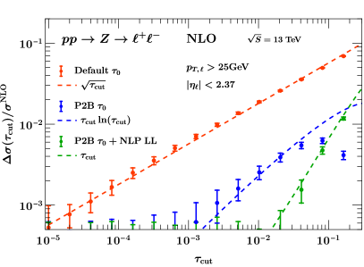
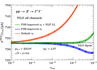
Figure -839: $Z\to\ell^{+}\ell^{-}$ at NLO: The left plot shows the slicing residual $\Delta\sigma$ for $0$-jettiness subtractions and improvements thereon. The right plot shows the total cross-sections and a comparison to the local subtraction result. Interpolation and scaling lines are shown to guide the eye.

We compute the slicing residual from the difference of the NLO cross-section computed using local dipole subtraction and the one calculated in $0-$jettiness subtractions at a given value of the ${\tau_{\text{cut}}}$ parameter.

Our numerical findings are shown in fig. -839 (left). We see that the default procedure suffers from fiducial $\sqrt{{\tau_{\text{cut}}}}$ power corrections, i.e. $p=1/2$, but that after using the P2B prescription these are removed and linear ${\tau_{\text{cut}}}$ scaling of the slicing residual is restored. This is in agreement with the findings of ref. Ebert:2019zkb . Once the fiducial power corrections are removed with P2B, the next-to-leading-power leading-logarithmic (NLP LL) corrections that are computed without fiducial cuts can be properly included, see section 2.2. They lead to a substantial further decrease in the size of the residual. The impact of the slicing residual on the calculation of the total NLO cross-section in each of these scenarios is summarized in fig. -839 (right).

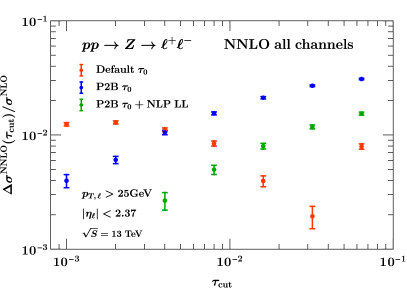
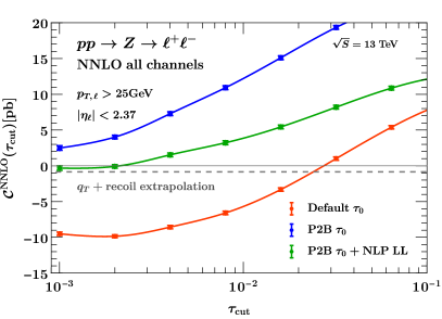
Figure -838: $Z\to\ell^{+}\ell^{-}$ at NNLO: The left plot shows $\Delta\sigma$ for various subtraction methods and improvements thereon. The right plot shows the total cross-section coefficients ($\mathcal{C}_{\text{NNLO}}{}$) and a comparison to the result obtained with $q_{T}$ subtractions with recoil.

The situation at NNLO is summarized in fig. -838. While no convergence is apparent at all for the default $0$-jettiness slicing, which suffers from sizable $\sqrt{{\tau_{\text{cut}}}}$ power corrections, the P2B corrections allow for cross-sections with per-mille level cutoff truncation errors. Our reference result is computed using $q_{T}$-subtractions with recoil power corrections and is shown as the dashed line. This result is obtained from a calculation using $q_{T\text{cut}}/Q=0.003$ that is in full agreement channel-by-channel with the corresponding result from Matrix Grazzini:2017mhc ; Buonocore:2021tke , as reported in Table 1.

$pp\to Z\to\ell^{+}\ell^{-}$ NNLO coefficient	$q\bar{q}+qq^{\prime}$	$qg$	$gg$
MCFM $q_{T}$ + recoil	$48\,732\pm 316$ fb	$-31\,819\pm 175$ fb	$13\,870\pm 25$ fb
Matrix $q_{T}$ + recoil	$48\,695\pm 364$ fb	$-31\,798\pm 131$ fb	$13\,786\pm 205$ fb
Relative Difference	$0.08\pm 0.99$ %	$0.07\pm 0.69$ %	$0.61\pm 1.53$ %

Table 1: Comparison of NNLO corrections to the total fiducial $Z$ cross-section obtained via Matrix and MCFM using $q_{T}$ subtractions with a recoil prescription. Results are broken down by different partonic channels.

The inclusion of the NLP LL corrections further improves the 0-jettiness result, leading to asymptotic flat results already at ${\tau_{\text{cut}}}=10^{-3}$. For example, in practical applications one might aim for an accuracy of better than $0.5\%$ on the total NNLO cross-section, corresponding to $\sigma^{\text{NNLO}{}}\times 0.005=$733\text{\,}\mathrm{p}\mathrm{b}$\times 0.005\sim$3.5\text{\,}\mathrm{p}\mathrm{b}$$. This cannot be obtained with the unimproved jettiness methods (nor $q_{T}$ subtractions) without a ${\tau_{\text{cut}}}$ value well below $10^{-4}$, which requires an extraordinary amount of computational effort and begins to enter the regime of numerical instability for double precision calculations. However, when using P2B-improved jettiness subtractions it can be reached using ${\tau_{\text{cut}}}\sim 2\times 10^{-3}$. After including NLP LL corrections, ${\tau_{\text{cut}}}\sim 10^{-2}$ suffices.

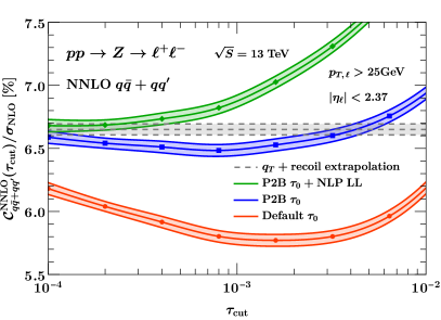
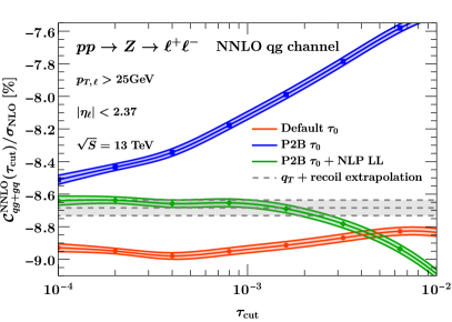
Figure -837: $Z\to\ell^{+}\ell^{-}$: Dependence of the NNLO total cross-section coefficient ($\mathcal{C}_{\text{NNLO}}{}$) on various subtraction improvements for the quark channel (left) and quark-gluon channel (right). The gluon-gluon channel is smaller and its plot is left out here, but is included in the overall result in fig. -838.

In order to gain further insight into the behavior of the power corrections, we also analyze the calculation of the NNLO coefficient in two different combinations of channels: the $qg$ and the $q\bar{q}+qq^{\prime}$ channels. This is especially instructive since the overall pattern observed in fig. -838 is obscured by the fact that the NNLO coefficient is very small. The breakdown into the two channels is shown in fig. -837. Again, we see that the removal of fiducial power corrections through the P2B subtractions significantly reduces the dependence on ${\tau_{\text{cut}}}$. We further observe that the NLP LL terms dramatically improve the convergence in the off-diagonal channel $qg$. This is the channel with the largest power corrections for this process and it therefore drives the improvement seen when including NLP LL corrections in fig. -838.

For the diagonal channel the NLP LL terms do not improve the size of the residual here, but they simply break the degeneracy that creates the erroneous plateau around ${\tau_{\text{cut}}}\sim 10^{-3}$. If, as in this case, the difference to the P2B-improved result is large one could use this as a diagnostic to avoid being misled by a local extremum. Overall, the size of the NLP LL contributions can be used as another way to quantify the size of the slicing residual. The NLP LL terms can also play an important role when asymptotically small values cannot be directly reached, but one instead has to rely on an extrapolation fit, for example in the case of limited computing resources or at higher orders. The additional simplification from removing the NLP LL terms in the extrapolation formula can allow for improved asymptotic fits and a more precise extraction of subleading logarithmic terms.

3.1.1 $Z$ rapidity distribution

Having established the improvements of the P2B-$\tau_{0}$ subtractions on the total cross-section, we now look at the rapidity distribution of the dilepton pair as an example of a more differential distribution.

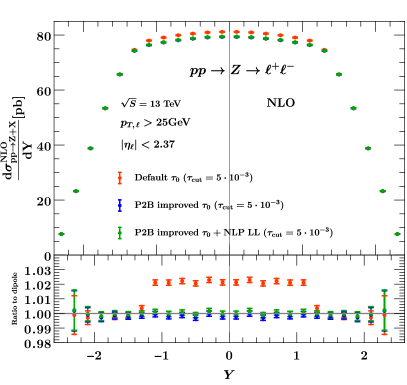
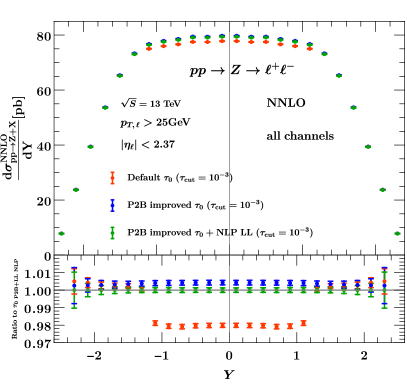
Figure -836: $Z\to\ell^{+}\ell^{-}$: $Z$ rapidity distribution with symmetric lepton cuts at NLO (left) and NNLO (right).

Results for the total $Z$ rapidity distribution at NLO are shown in fig. -836 (left plot) for ${\tau_{\text{cut}}}=5\cdot 10^{-3}$. We observe that the convergence with P2B-$\tau_{0}$ subtractions is excellent. In fig. -835 we show the slicing residuals at NLO for the different methods. We observe remarkable precision with the inclusion of P2B corrections and further improvements when NLP LL corrections are accounted for.

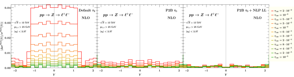
Figure -835: $Z\to\ell^{+}\ell^{-}$: rapidity distribution residuals at NLO. Each line corresponds to a different value of the cut parameter and represents the residual error as a function of Y, normalized to the NLO distribution calculated using dipole subtraction.

Results for the total $Z$ rapidity distribution at NNLO are shown in fig. -836 (right plot) for ${\tau_{\text{cut}}}=10^{-3}$. We see that without the P2B corrections the size of the slicing residual is about 2%, flat across the distribution. Once these are included the remaining correction from the inclusion of NLP LL terms is less than half a percent, again flat in $Y$.

To better understand the ${\tau_{\text{cut}}}$-dependence of the total rapidity distribution we again present results in the different channels at NNLO in fig. -834. We observe that the convergence of each separate channel is improved using P2B-$\tau_{0}$ subtraction but that the NLP LL corrections are especially important for the $qg$ channel, as already observed for the total cross-section. Note that the $gg$ channel does not receive any such corrections at this order.

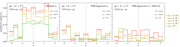
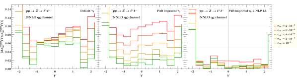
Figure -834: $Z\to\ell^{+}\ell^{-}$: $Z$ rapidity distribution residuals at NNLO, for the $q\bar{q}+qq^{\prime}$ channel (top) and $qg$ channel (bottom).

3.2 Higgs production

We consider Higgs production with decay into a photon pair, $H\to\gamma\gamma$, with a representative set of cuts:

$$p_{T,\gamma}^{\rm hard}>$40\text{\,}\mathrm{G}\mathrm{e}\mathrm{V}$\,,\qquad p_{T,\gamma}^{\rm soft}>$30\text{\,}\mathrm{G}\mathrm{e}\mathrm{V}$\,,\qquad\left|\eta_{\gamma}\right|<2.37\,.$$ (21)

The scaling behavior of the slicing residual at NLO is shown in fig. -833 (left). Including the P2B corrections changes the scaling from $p=1/2$ to $p=1$, as expected. Accounting for the NLP LL power corrections decreases the overall size of the residual error. The impact of these improvements on the NLO cross-section calculation is demonstrated in fig. -833 (right). For $0.1\%$ control of the NLO result one only needs ${\tau_{\text{cut}}}\sim 5\times 10^{-3}$ (P2B+NLP LL) rather than ${\tau_{\text{cut}}}\sim 10^{-5}$ (unimproved).

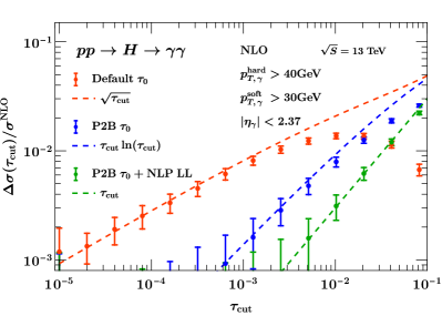
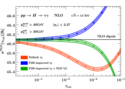
Figure -833: $H\to\gamma\gamma$ at NLO: The left plot shows the slicing residual $\Delta\sigma$ for various subtraction method improvements. The right plot shows the total cross-sections and a comparison to the local subtraction result. Interpolation lines are shown to guide the eye.

At NNLO we obtain the results shown in fig. -832. It is clear that, without the inclusion of any improvements, the default calculation has a large residual error and is only just beginning to enter the region of asymptotic scaling. After inclusion of P2B corrections the calculation is clearly in the asymptotic regime, with further improvement in scaling after accounting for the NLP LL corrections. These effects obviously result in significant improvements in the calculation of the NNLO coefficient, as shown in fig. -832 (right). In this case the inclusion of NLP LL corrections does not lead to substantial numerical improvements because the size of the power corrections accounted for by the P2B scheme is already quite large.

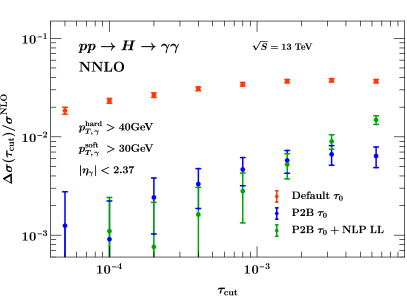
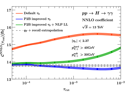
Figure -832: $H\to\gamma\gamma$ at NNLO: The left plot shows the slicing residual $\Delta\sigma$ for various subtraction method improvements. The right plot shows the total cross-section coefficients ($\mathcal{C}_{\text{NNLO}}{}$).

3.2.1 Higgs rapidity distribution

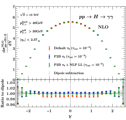
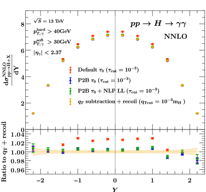
Figure -831: $H\to\gamma\gamma$: Higgs rapidity distribution at NLO (left) and NNLO (right), computed using ${\tau_{\text{cut}}}=10^{-3}$ in the default, P2B and P2B+NLP LL schemes.

We now turn to a more differential quantity, the Higgs rapidity distribution. In fig. -831 we show the total result at NLO and NNLO for ${\tau_{\text{cut}}}=10^{-3}$ in the different approaches. At NNLO the unimproved result shows a flat slicing residual of about 3%. Once P2B corrections are included, the distribution agrees with our $q_{T}$+recoil reference result within numerical errors. Improvements from including NLP LL terms are small at the given ${\tau_{\text{cut}}}$.

A similar picture emerges by looking at the slicing residuals at NLO and at NNLO for various values of the cut parameters, which are shown in fig. -830 and fig. -829, respectively. At NLO the residuals are computed relative to the local dipole subtraction, while at NNLO our reference is the calculation that employs P2B and includes NLP LL corrections with ${\tau_{\text{cut}}}=10^{-4}$.

As expected from the discussion of the total cross-section, there is significant improvement in convergence when using the P2B corrections. At NLO, for ${\tau_{\text{cut}}}=10^{-3}$ the residual error is approximately flat at 1% in the unimproved case, a couple per mille once P2B corrections are included, then completely negligible (within numerical uncertainties) after including NLP LL effects. At NNLO we see again that the P2B corrections provide a huge improvement in the convergence, with a more modest further gain after accounting for NLP LL terms.

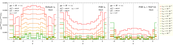
Figure -830: $H\to\gamma\gamma$: residual errors in the Higgs rapidity distribution at NLO, computed by comparing to a calculation performed using local dipole subtraction.

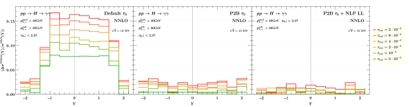
Figure -829: $H\to\gamma\gamma$: residual errors on the Higgs rapidity distribution at NNLO. Each line corresponds to a different value of the cut parameter and represents the residual error as a function of $y$, where the reference calculation is the one using P2B and NLP LL terms at ${\tau_{\text{cut}}}=10^{-4}$.

4 Di-photon production at NNLO with $\text{P2B}_{\gamma}$ $\tau_{0}$ and $\text{P2B}_{\gamma}~{}q_{T}$ subtractions

The P2B method described in the previous sections directly captures fiducial power corrections for color-singlet processes. However, for di-photon production with photon isolation, additional power corrections due to the isolation prescription contribute. The goal of this section is to understand how to incorporate some of these isolation power corrections into the subtraction term for the non-local subtractions, improving their precision for photon processes.

In sec. 4.1, we briefly review the behavior of power corrections for photon processes. Then in sec. 4.2, we discuss their interplay with P2B-improved subtractions and present $\text{P2B}_{\gamma}$-improved non-local subtractions, a new method to simultaneously incorporate kinematic power corrections and a set of isolation power corrections in the $\tau_{0}$ and $q_{T}$ subtractions.

4.1 Power corrections in the presence of photon isolation

In the case where photon isolation is included, the scaling of the power corrections depends on the isolation criterion in a non-trivial way. We consider Frixione’s isolation Frixione:1998jh for prompt photon production, with cone size $R$, exponent $n$, and transverse energy threshold $E_{T}^{\mathrm{iso}}$, which imposes the following requirement on the final state partons

$$\sum_{d(i,\gamma)\leq r}E_{T}^{i}\leq E_{T}^{\mathrm{iso}}\left[\frac{1-\cos(r)}{1-\cos(R)}\right]^{n}\,,\qquad\forall r\leq R\,.$$ (22)

Sometimes the isolation energy is taken as a fraction of the photon transverse momentum, in which case $E_{T}^{\mathrm{iso}}=\varepsilon^{\mathrm{iso}}p_{T}^{\gamma}$. The angular distance measure $d(i,\gamma)$ between photon and parton $i$ is defined via $d(i,\gamma)=\sqrt{(\eta_{i}-\eta_{\gamma})^{2}+(\phi_{i}-\phi_{\gamma})^{2}}$ with rapididies $\eta$ and azimuthal angles $\phi$.

Here one has to distinguish between the case of a quark or a gluon in the isolation cone. The case of a gluon in the isolation cone has been extensively discussed at NLO in ref. Ebert:2019zkb . In the case of a quark (the actual fragmentation case), this smooth isolation prescription ensures the QCD infrared-safe removal of the collinear quark-photon singularity. The scaling of the power corrections in this case has been derived at NLO in ref. Becher:2020ugp . Generally one expects the scaling behavior to be similar at NNLO, but this has not been studied in detail so far.

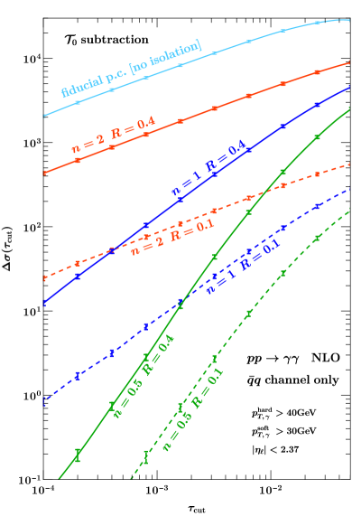
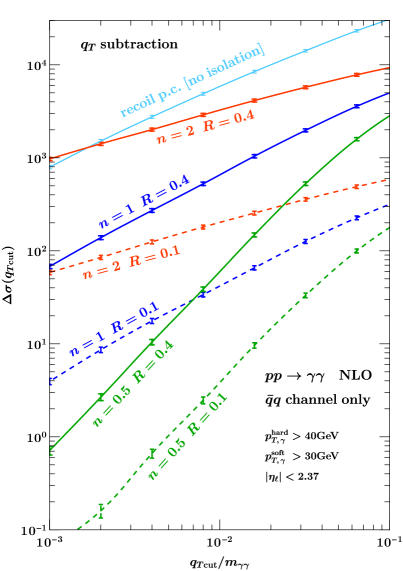
Figure -828: Difference between the P2B correction with and without isolation for different isolation parameters at NLO for the $q\bar{q}$ channel. Left: $0$-jettiness, right: $q_{T}$. For comparison we also plot the P2B correction without isolation. Note that the choice of colors in this figure is not related to the one in eq. (26).

For a gluon, taking $R\ll 1$ and for $n\geq 1/2$, at NLO one has Ebert:2019zkb ; Becher:2020ugp

$$\text{gluon:}\qquad\Delta\sigma^{\mathrm{fiducial}}_{\mathrm{Frixione-iso}}({x_{\text{cut}}})\sim\begin{cases}R^{2}\sqrt[n]{{\mathcal{T}_{0\,\text{cut}}}/E_{T}^{\mathrm{iso}}}&\text{0-jettiness subtraction}\\ R^{2}\sqrt[n]{q_{T\mathrm{cut}}/E_{T}^{\mathrm{iso}}}&q_{T}\text{-subtraction}\end{cases}$$ (23)

or equivalently,

$$\text{gluon:}\qquad\Delta\sigma^{\mathrm{fiducial}}_{\mathrm{Frixione-iso}}({x_{\text{cut}}})\sim\begin{cases}R^{2}\sqrt[n]{{x_{\text{cut}}}}\sqrt[n]{Q/E_{T}^{\mathrm{iso}}}&\text{0-jettiness subtraction}\\ R^{2}\sqrt[2n]{{x_{\text{cut}}}}\sqrt[n]{Q/E_{T}^{\mathrm{iso}}}&q_{T}\text{-subtraction}\,.\end{cases}$$ (24)

Here $Q$ is a hard scale of the process which is typically taken to be $m_{\gamma\gamma}$, the invariant mass of the di-photon pair.

To test eq. (24), we have calculated the difference of the P2B correction for $q\bar{q}\to\gamma\gamma$ cross-sections at NLO with and without isolation for different isolation parameters using $\tau_{0}$ and $q_{T}$ subtraction as a function of the cut parameter. The results are presented in fig. -828 and show that the $n$-dependence follows eq. (24). Moreover, as indicated, we see that changing the cone radius only impacts the overall size of the power correction but not its cutoff-scaling behavior.

In the fragmentation case for a quark, at NLO one has

$$\text{quark:}\qquad\Delta\sigma^{\mathrm{fiducial}}_{\mathrm{Frixione-iso}}\sim\begin{cases}\frac{{\mathcal{T}_{0\,\text{cut}}}}{Q}\log(R)&\text{0-jettiness subtraction}\\ \frac{q_{T\mathrm{cut}}}{Q}\log(R)&q_{T}\text{-subtraction}\,.\end{cases}$$ (25)

The scaling in the $q_{T}$ subtraction case has been derived analytically in ref. Becher:2020ugp while we have determined the equivalent for jettiness subtractions numerically.

The net result is that in the sum of all partonic channels, where both gluon and quark final states contribute, linear power corrections will always be present, irrespective of the value of $n$ that determines the scaling for the gluonic case. Typically, due to the scaling in $R$, the quark fragmentation power corrections dominate for small $R$, even when $n>1$.

Overall power corrections.

Taking Frixione isolation with $n=1$ as an example, the sum of the hadronic, fiducial and photon isolation power corrections is as follows,

$$\Delta\sigma^{\mathrm{fiducial}+\mathrm{hadronic}}_{p_{T}^{\gamma}+\mathrm{iso},n=1}\sim\begin{cases}{\color[rgb]{1,0,0}\sqrt{\frac{{\mathcal{T}_{0\,\text{cut}}}}{Q}}}+{\color[rgb]{0,0,1}\frac{{\mathcal{T}_{0\,\text{cut}}}}{Q}\,R^{2}\frac{Q}{E_{T}^{\mathrm{iso}}}+\frac{{\mathcal{T}_{0\,\text{cut}}}}{Q}\log(R)}+{\color[rgb]{0,.6,0}\frac{{\mathcal{T}_{0\,\text{cut}}}}{Q}}\,,&\text{0-jettiness subtraction}\\[14.22636pt] {\color[rgb]{1,0,0}\frac{q_{T\mathrm{cut}}}{Q}}+{\color[rgb]{0,0,1}\frac{q_{T\mathrm{cut}}}{Q}\,R^{2}\frac{Q}{E_{T}^{\mathrm{iso}}}+\frac{q_{T\mathrm{cut}}}{Q}\log(R)}+{\color[rgb]{0,.6,0}\frac{q^{2}_{T\mathrm{cut}}}{Q^{2}}}\,,&q_{T}\text{-subtraction}\end{cases}$$ (26)

where we have ignored the logarithmic ${\tau_{\text{cut}}}$ and $q_{T\text{cut}}$ behavior for brevity and have indicated the contributions coming from generic $p_{T}^{\gamma}$ cuts, photon isolation cuts, and hadronic/dynamical power corrections with different colors. Note that power corrections for fiducial leptonic and photon isolation cuts have only been analyzed at NLO Ebert:2019zkb ; Becher:2020ugp , although these corrections are expected to be dominant at higher orders as well. Further, as mentioned in sec. 2.2, the scaling of the hadronic power corrections (green in eq. (26)) is based on a Drell-Yan analysis. A generalization has yet to be demonstrated in the literature, in particular for non-Born channels at higher orders.

Before moving on we now summarize the discussion of power corrections in sec. 2.2 and here. We highlight the following:

• In general, fiducial power corrections due to the kinematic cuts on the transverse momentum of the final state leptons (or photons, e.g. for $H\to\gamma\gamma$ in gluon fusion), scale as $\mathcal{O}(\sqrt{{x_{\text{cut}}}})$, therefore dominating over the hadronic ones, which scale as $\mathcal{O}({x_{\text{cut}}})$.

• In the presence of photon isolation, power corrections are overall dominated by the fragmentation contribution with a quark in the final state. These further dominate over all other power corrections due to the $\log(R)$ scaling.
  For the gluonic channel there is a strong dependence of the power corrections on the isolation parameters and the subtraction method. For example, with $n=1$ these isolation power corrections are important and behave as a leading source of power correction for $q_{T}$-subtraction, while for 0-jettiness they have a smaller impact, comparable to that of hadronic power corrections.

• In scenarios where multiple scales are at play, power corrections to slicing schemes can acquire dependence on several of these scales. Even for the simple case of color singlet production, as one turns on fiducial cuts, the power corrections may depend on scales such as $E_{T}^{\mathrm{iso}}$, $R$, etc. While these scales formally enter as $\mathcal{O}(1)$ parameters, they strongly change the numerical impact of power correction compared to a naive analysis of linear or quadratic scaling. It is therefore of paramount importance to be able to treat them systematically.

4.2 Capturing fragmentation power corrections

A crucial difference between di-photon production with photon isolation and Drell-Yan processes is that, when quarks are produced in the final state, the inclusive cross-section is ill-defined in perturbation theory in the absence of an isolation criterion or a non-perturbative object such as a fragmentation function. For example, in $q_{T}$ subtractions with a recoil prescription for fiducial power corrections, it is clear that no photon isolation power corrections can be captured given that it only operates at the Born kinematics level. While a naive application of the P2B prescription is also not effective, as we describe below, the access to the full matrix element allows modifications of the scheme to capture a set of these power corrections.

To be more precise, in the case of the emission of a gluon into the isolation cone the P2B prescription works as expected, as the inclusive cross-section is well defined even in the absence of an isolation criterion. With the isolation removing the gluon emission’s phase space that is collinear to the photon, the soft-gluon singularity is canceled between $\mathcal{O}$ and $\mathcal{\tilde{O}}$ in the P2B prescription, leaving behind a finite power correction that is captured. In section 4.3 we demonstrate numerically that the P2B-improvements in this case follow the expected power behavior and magnitude. The power corrections from the P2B terms match the power corrections obtained from a recoil prescription in $q_{T}$ subtractions.

On the other hand, in the case of the emission of a quark, the isolation prescription takes care of removing the collinear quark-photon singularity. As the quark becomes soft the isolation ceases to act, but no soft QCD singularity arises as the soft quark emission is power suppressed. A source of slicing residual is that in the slicing calculation such a contribution is neglected when the quark energy is smaller than the cut parameter. Fortunately, we can correct for this effect in a simple way. In realistic scenarios the photon has some transverse momentum cuts and, combined with the isolation, this implies that every quark that is close to the photon must be soft. Even below the cut, such quarks don’t need any P2B counterterm because their matrix element is not singular. This implies that we can account for this effect by simply turning off the P2B counterterm in the cone of radius $R$ around the photon. We demonstrate in section 4.3 that this procedure significantly improves the overall convergence, hence capturing a significant portion of the isolation power corrections.

Since this is a prescription for one emission, we apply it at NLO and for the NNLO real-virtual corrections with a quark emission. Further adjustments should be necessary to handle the double emission contributions and require further study. Nevertheless, we find that the prescription presented here significantly improves the cutoff dependence at NNLO even if just applied to the real-virtual corrections, as presented in the results section. We refer to this improved scheme as $\text{P2B}_{\gamma}$ subtractions, distinguishing it from the normal P2B improved subtractions which do not include this prescription.

4.3 Numerical results

Following our discussion of photon-isolation power corrections, in this section we demonstrate the improvements from the $\text{P2B}_{\gamma}$-subtraction for di-photon production. We use photon cuts as in $H\to\gamma\gamma$: $p_{T,\gamma}^{\rm hard}>$40\text{\,}\mathrm{G}\mathrm{e}\mathrm{V}$$, $p_{T,\gamma}^{\rm soft}>$30\text{\,}\mathrm{G}\mathrm{e}\mathrm{V}$$, $\left|\eta_{\gamma}\right|<2.37$ and Frixione photon isolation as in eq. 22 with $E_{T}^{\text{iso}}=$10\text{\,}\mathrm{GeV}$$, $R=0.4$, and $n=1$. We show results for a center-of-mass energy $\sqrt{s}=$13\text{\,}\mathrm{GeV}$$ with the PDF set NNPDF31_nnlo_as_0118 NNPDF:2017mvq . The factorization and renormalization scales are set to the invariant mass $Q$ of the di-photon system. Because the distinction between final-state gluons (P2B) and quarks ($\text{P2B}{}_{\gamma}$) is crucial for the discussion of different schemes, we separate the $q\bar{q}+qq^{\prime}$ and $qg$ (fragmentation) channels in our initial discussion.

Note that in all cases the smallest $q_{T,\text{cut}}$ and ${\tau_{\text{cut}}}$ are as low as can be achieved using numerical double precision, even using an improved treatment of all matrix elements in MCFM Bothmann:2024hgq . Smaller values of $q_{T,\text{cut}}$ and ${\tau_{\text{cut}}}$ would require technical cutoffs that have an impact on the slicing cut itself. As will become clear, the inclusion of power corrections in the photon isolation itself is essential to achieve a reliable result.

In fig. -827 we first consider the $q\bar{q}+qq^{\prime}$ channels. Note that this channel doesn’t receive $\text{P2B}{}_{\gamma}$ improvements since there is only a gluon in the final state for the real-virtual contribution. We observe that the corrections from P2B in $\tau_{0}$ and recoil in $q_{T}$ are substantial and allow asymptotic behavior to be reached much faster. This is in line with previous observations for $q_{T}$ subtractions in Matrix Buonocore:2021tke .

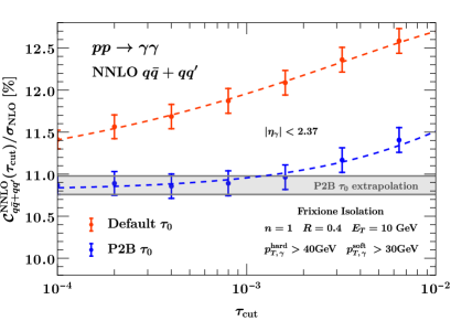
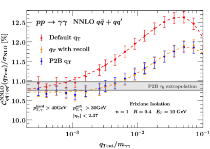
Figure -827: NNLO coefficient K-factor for di-photon production, $q\bar{q}+qq^{\prime}$ channel only, for $0$-jettiness (left) and $q_{T}$ subtractions (right) and their improved versions.

In fig. -826 we consider the $qg$ fragmentation channels. In this channel a quark in the final state is always present and an isolation procedure is required to define a finite cross-section. Here we distinguish between P2B improvements and $\text{P2B}{}_{\gamma}$ improvements. Looking first at the $q_{T}$ subtraction results in fig. -826 (right) we see numerically equal improvements from the recoil and P2B power corrections, as expected. Unlike for the Born channel, they are small and do not help noticeably. This issue is again in line with the findings in the literature Buonocore:2021tke . No reliable result can be obtained, even with power corrections from recoil, in stark contrast to the cases of $Z$ and $H$ production.

The power corrections associated with the photon isolation itself are dominant, and these are not captured by a recoil or P2B approach. On the other hand the $\text{P2B}{}_{\gamma}$ improvements seen in fig. -826 are substantial. It stands out that, compared to the non-fragmentation channel, the $\tau_{0}$ subtractions perform substantially better than $q_{T}$ subtractions, reaching asymptotics already for ${\tau_{\text{cut}}}<10^{-4}$ down to the smallest value $5\cdot 10^{-6}$ that can be achieved in double precision numerics. The huge improvements comparing the nominal slicing procedure to the new $\text{P2B}{}_{\gamma}$ scheme are the same for $q_{T}$ and $\tau_{0}$ subtractions. For both slicing variables the $\text{P2B}{}_{\gamma}$ procedure includes a sizable class of ${x_{\text{cut}}}$-linear power corrections.

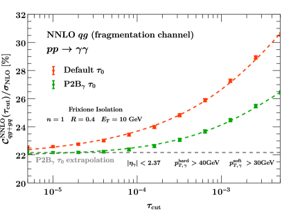
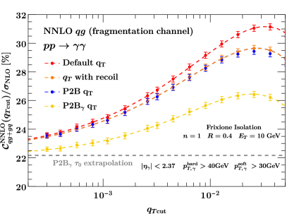
Figure -826: NNLO coefficient K-factor for di-photon production, $qg$ fragmentation channel only, for $0$-jettiness (left) and $q_{T}$ subtractions (right) and their improved versions.

Finally, the sum of all channels (including the $gg$ component) is presented in fig. -825, where we have used a fitted asymptotic extrapolation to continue the $q\bar{q}+qq^{\prime}$ channel down to ${\tau_{\text{cut}}}=5\cdot 10^{-6}$ for $0$-jettiness (it is already asymptotically flat at ${\tau_{\text{cut}}}=10^{-3}$, as can be seen in fig. -827). We performed asymptotic fits based on the two to three dominant subleading terms of the expected power corrections as laid out in section 4.1. For $q_{T}$ subtractions with or without recoil improvements we observe that the asymptotic extrapolation has large uncertainties given that the distribution has not plateaued. On the other hand a robust asymptotic extraction is possible using $\text{P2B}{}_{\gamma}+q_{T}$ and $0$-jettiness subtractions. In our study, the most reliable result is achieved by adding the $\text{P2B}{}_{\gamma}$ corrections to $0$-jettiness subtractions. There one additionally reaps the benefit in the fragmentation channel of a better intrinsic scaling compared to $q_{T}$. The results achievable in double precision reach well into the asymptotic flat region, such that the constant piece in the asymptotic fit is well constrained.

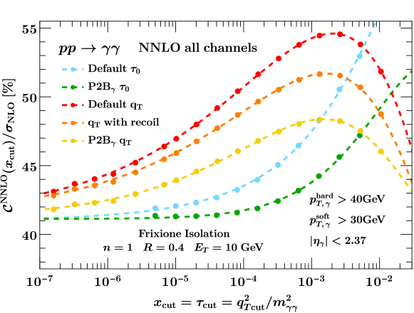
Figure -825: NNLO coefficient K-factor for di-photon production for $0$-jettiness and $q_{T}$ subtractions and their improved versions. Asymptotic fits take into account two to three subleading terms.

5 Conclusions

The LHC has enabled the measurement of many Standard Model processes with a high precision, challenging theoretical predictions that rely on continued developments in higher-order calculations. The continuation of this program with the HL-LHC will significantly raise these challenges for the whole high-energy collider physics community, but is expected to result in significant scientific, technological and societal advancements.

One particularly important aspect of theoretical predictions is the combination of individually infrared divergent higher-order amplitudes into a finite cross-section that can be compared with experimental measurements. These subtraction methods are developed order by order in perturbation theory, and several different methods exist with individual benefits and drawbacks.

In this paper we have introduced P2B-improved $0$-jettiness and $q_{T}$ subtraction methods in the code MCFM. The P2B-improved scheme Ebert:2019zkb includes power corrections that arise in the presence of fiducial cuts on the color-singlet system and are typically dominant compared to other subleading-power corrections. With these power corrections accounted for, much more reliable and robust results can be obtained. We exemplified the implementation for $Z$-boson production in the case of symmetric lepton cuts, and for Higgs production. Both for total cross-section rates as well as for rapidity distributions we find dramatic improvements in the processes examined, both at NLO and NNLO. We find that the P2B-$q_{T}$ method captures the same $\mathcal{O}(q_{T,\text{cut}})$ power corrections as the recoil prescription for these Drell-Yan-type processes. In the case of $0$-jettiness the P2B-improvements allow one to additionally benefit, in the presence of realistic experimental cuts, from the analytically computed leading-logarithmic hadronic power corrections Moult:2016fqy ; Moult:2017jsg ; Ebert:2018lzn , further improving the calculation of predictions.

For processes with photon isolation an additional source of power corrections arises due to the isolation procedure. These power corrections are typically large and dominant among the fiducial power corrections. In the non-fragmentation channel we find large improvements with both P2B schemes, and also the recoil scheme in the case of $q_{T}$ subtractions. In the numerically dominant fragmentation channel, where the collinear photon-quark singularity is removed, we find that the P2B corrections (and recoil in the case of $q_{T}$ subtractions) are ineffective. The dominant set of power corrections is not removed by this procedure. In the case of $q_{T}$ subtractions with a recoil this can be readily understood, since the power correction procedure does not take into account any information from the isolation prescription itself.

For this numerically-dominant fragmentation channel we developed a method, $\text{P2B}{}_{\mathbf{\gamma}}$, to include the bulk of photon-isolation power corrections. We numerically studied this for di-photon production, finding that it significantly improved the calculation and enabled reliable and robust results in the presence of photon isolation. Additionally, we found that in the fragmentation channel the isolation power corrections of $0$-jettiness are substantially better than $q_{T}$-subtractions (compared to the non-fragmentation channels). The combination of intrinsically better power corrections and the photon-isolation-improved $\text{P2B}{}_{\gamma}$ scheme allows us to extract a reliable result even without the need for extrapolation. We demonstrate asymptotically flat behavior for over an order of magnitude in the cutoff parameter. Without these improvements a significant cutoff dependence is present even for very small values of the cutoff, making the extraction of a result with an error less than a few percent challenging to obtain.

The P2B and $\text{P2B}_{\gamma}$ power corrections presented in this paper will be made available in the upcoming 10.4 release of MCFM and complement and improve upon the existing recoil power corrections for $q_{T}$ subtractions.

- (1) CMS collaboration, A. M. Sirunyan et al., Precision luminosity measurement in proton-proton collisions at 13 TeV in 2015 and 2016 at CMS, Eur. Phys. J. C 81 (2021) 800, [arXiv:2104.01927].
- (2) ATLAS collaboration, G. Aad et al., Luminosity determination in collisions at TeV using the ATLAS detector at the LHC, Eur. Phys. J. C 83 (2023) 982, [arXiv:2212.09379].
- (3) ATLAS collaboration, G. Aad et al., Precise measurements of - and -boson transverse momentum spectra with the ATLAS detector using collisions at TeV and TeV, arXiv:2404.06204.
- (4) CMS collaboration, A. M. Sirunyan et al., Measurements of differential Z boson production cross sections in proton-proton collisions at = 13 TeV, JHEP 12 (2019) 061, [arXiv:1909.04133].
- (5) ATLAS collaboration, G. Aad et al., Measurement of the transverse momentum distribution of Drell–Yan lepton pairs in proton–proton collisions at TeV with the ATLAS detector, Eur. Phys. J. C 80 (2020) 616, [arXiv:1912.02844].
- (6) ATLAS collaboration, G. Aad et al., Measurements of the Higgs boson inclusive and differential fiducial cross-sections in the diphoton decay channel with pp collisions at = 13 TeV with the ATLAS detector, JHEP 08 (2022) 027, [arXiv:2202.00487].
- (7) ATLAS collaboration, G. Aad et al., Measurement of the total and differential Higgs boson production cross-sections at = 13 TeV with the ATLAS detector by combining the H → ZZ∗→ 4 and H → decay channels, JHEP 05 (2023) 028, [arXiv:2207.08615].
- (8) CMS collaboration, A. Hayrapetyan et al., Measurements of inclusive and differential cross sections for the Higgs boson production and decay to four-leptons in proton-proton collisions at = 13 TeV, JHEP 08 (2023) 040, [arXiv:2305.07532].
- (9) ATLAS collaboration, G. Aad et al., Measurement of the and cross-sections in pp collisions at TeV with the ATLAS detector, Eur. Phys. J. C 84 (2024) 78, [arXiv:2306.11379].
- (10) ATLAS, CMS collaboration, Addendum to the report on the physics at the HL-LHC, and perspectives for the HE-LHC: Collection of notes from ATLAS and CMS, CERN Yellow Rep. Monogr. 7 (2019) Addendum, [arXiv:1902.10229].
- (11) ATLAS collaboration, Snowmass White Paper Contribution: Physics with the Phase-2 ATLAS and CMS Detectors, .
- (12) S. Frixione and G. Ridolfi, Jet photoproduction at HERA, Nucl. Phys. B 507 (1997) 315–333, [hep-ph/9707345].
- (13) G. P. Salam and E. Slade, Cuts for two-body decays at colliders, JHEP 11 (2021) 220, [arXiv:2106.08329].
- (14) X. Chen, T. Gehrmann, E. W. N. Glover, A. Huss, B. Mistlberger and A. Pelloni, Fully Differential Higgs Boson Production to Third Order in QCD, Phys. Rev. Lett. 127 (2021) 072002, [arXiv:2102.07607].
- (15) G. Billis, B. Dehnadi, M. A. Ebert, J. K. L. Michel and F. J. Tackmann, Higgs pT Spectrum and Total Cross Section with Fiducial Cuts at Third Resummed and Fixed Order in QCD, Phys. Rev. Lett. 127 (2021) 072001, [arXiv:2102.08039].
- (16) X. Chen, T. Gehrmann, N. Glover, A. Huss, T.-Z. Yang and H. X. Zhu, Dilepton Rapidity Distribution in Drell-Yan Production to Third Order in QCD, Phys. Rev. Lett. 128 (2022) 052001, [arXiv:2107.09085].
- (17) X. Chen, T. Gehrmann, E. W. N. Glover, A. Huss, P. F. Monni, E. Re et al., Third-Order Fiducial Predictions for Drell-Yan Production at the LHC, Phys. Rev. Lett. 128 (2022) 252001, [arXiv:2203.01565].
- (18) X. Chen, T. Gehrmann, N. Glover, A. Huss, T.-Z. Yang and H. X. Zhu, Transverse mass distribution and charge asymmetry in W boson production to third order in QCD, Phys. Lett. B 840 (2023) 137876, [arXiv:2205.11426].
- (19) T. Neumann and J. Campbell, Fiducial Drell-Yan production at the LHC improved by transverse-momentum resummation at N4LLp+N3LO, Phys. Rev. D 107 (2023) L011506, [arXiv:2207.07056].
- (20) J. Campbell and T. Neumann, Third order QCD predictions for fiducial W-boson production, JHEP 11 (2023) 127, [arXiv:2308.15382].
- (21) F. Devoto, K. Melnikov, R. Röntsch, C. Signorile-Signorile and D. M. Tagliabue, A fresh look at the nested soft-collinear subtraction scheme: NNLO QCD corrections to N-gluon final states in annihilation, JHEP 02 (2024) 016, [arXiv:2310.17598].
- (22) X. Chen, T. Gehrmann, E. W. N. Glover, A. Huss and M. Marcoli, Automation of antenna subtraction in colour space: gluonic processes, JHEP 10 (2022) 099, [arXiv:2203.13531].
- (23) G. Bertolotti, L. Magnea, G. Pelliccioli, A. Ratti, C. Signorile-Signorile, P. Torrielli et al., NNLO subtraction for any massless final state: a complete analytic expression, JHEP 07 (2023) 140, [arXiv:2212.11190]. [Erratum: JHEP 05, 019 (2024)].
- (24) W. J. Torres Bobadilla et al., May the four be with you: Novel IR-subtraction methods to tackle NNLO calculations, Eur. Phys. J. C 81 (2021) 250, [arXiv:2012.02567].
- (25) I. Moult, L. Rothen, I. W. Stewart, F. J. Tackmann and H. X. Zhu, Subleading Power Corrections for N-Jettiness Subtractions, Phys. Rev. D 95 (2017) 074023, [arXiv:1612.00450].
- (26) R. Boughezal, X. Liu and F. Petriello, Power Corrections in the N-jettiness Subtraction Scheme, JHEP 03 (2017) 160, [arXiv:1612.02911].
- (27) I. Moult, L. Rothen, I. W. Stewart, F. J. Tackmann and H. X. Zhu, N -jettiness subtractions for at subleading power, Phys. Rev. D 97 (2018) 014013, [arXiv:1710.03227].
- (28) R. Boughezal, A. Isgrò and F. Petriello, Next-to-leading-logarithmic power corrections for -jettiness subtraction in color-singlet production, Phys. Rev. D 97 (2018) 076006, [arXiv:1802.00456].
- (29) M. A. Ebert, I. Moult, I. W. Stewart, F. J. Tackmann, G. Vita and H. X. Zhu, Power Corrections for N-Jettiness Subtractions at , JHEP 12 (2018) 084, [arXiv:1807.10764].
- (30) M. A. Ebert, I. Moult, I. W. Stewart, F. J. Tackmann, G. Vita and H. X. Zhu, Subleading power rapidity divergences and power corrections for qT, JHEP 04 (2019) 123, [arXiv:1812.08189].
- (31) R. Boughezal, A. Isgrò and F. Petriello, Next-to-leading power corrections to jet production in -jettiness subtraction, Phys. Rev. D 101 (2020) 016005, [arXiv:1907.12213].
- (32) I. Moult, I. W. Stewart, G. Vita and H. X. Zhu, The Soft Quark Sudakov, JHEP 05 (2020) 089, [arXiv:1910.14038].
- (33) I. Moult, I. W. Stewart, G. Vita and H. X. Zhu, First Subleading Power Resummation for Event Shapes, JHEP 08 (2018) 013, [arXiv:1804.04665].
- (34) M. Beneke, M. Garny, S. Jaskiewicz, R. Szafron, L. Vernazza and J. Wang, Leading-logarithmic threshold resummation of Higgs production in gluon fusion at next-to-leading power, JHEP 01 (2020) 094, [arXiv:1910.12685].
- (35) Z. L. Liu and M. Neubert, Factorization at subleading power and endpoint-divergent convolutions in decay, JHEP 04 (2020) 033, [arXiv:1912.08818].
- (36) Z. L. Liu, B. Mecaj, M. Neubert and X. Wang, Factorization at subleading power, Sudakov resummation, and endpoint divergences in soft-collinear effective theory, Phys. Rev. D 104 (2021) 014004, [arXiv:2009.04456].
- (37) M. Beneke, M. Garny, S. Jaskiewicz, R. Szafron, L. Vernazza and J. Wang, Large-x resummation of off-diagonal deep-inelastic parton scattering from d-dimensional refactorization, JHEP 10 (2020) 196, [arXiv:2008.04943].
- (38) M. van Beekveld, E. Laenen, J. Sinninghe Damsté and L. Vernazza, Next-to-leading power threshold corrections for finite order and resummed colour-singlet cross sections, JHEP 05 (2021) 114, [arXiv:2101.07270].
- (39) M. Beneke, M. Garny, S. Jaskiewicz, J. Strohm, R. Szafron, L. Vernazza et al., Next-to-leading power endpoint factorization and resummation for off-diagonal “gluon” thrust, JHEP 07 (2022) 144, [arXiv:2205.04479].
- (40) Z. L. Liu, M. Neubert, M. Schnubel and X. Wang, Factorization at next-to-leading power and endpoint divergences in gg → h production, JHEP 06 (2023) 183, [arXiv:2212.10447].
- (41) G. Ferrera, W.-L. Ju and M. Schönherr, Zero-bin subtraction and the qT spectrum beyond leading power, JHEP 04 (2024) 005, [arXiv:2312.14911].
- (42) G. Vita, N3LO power corrections for 0-jettiness subtractions with fiducial cuts, JHEP 07 (2024) 241, [arXiv:2401.03017].
- (43) M. Beneke, Y. Ji and X. Wang, Renormalization of the next-to-leading-power → h and gg → h soft quark functions, JHEP 05 (2024) 246, [arXiv:2403.17738].
- (44) M. Cacciari, F. A. Dreyer, A. Karlberg, G. P. Salam and G. Zanderighi, Fully Differential Vector-Boson-Fusion Higgs Production at Next-to-Next-to-Leading Order, Phys. Rev. Lett. 115 (2015) 082002, [arXiv:1506.02660]. [Erratum: Phys.Rev.Lett. 120, 139901 (2018)].
- (45) M. A. Ebert and F. J. Tackmann, Impact of isolation and fiducial cuts on qT and N-jettiness subtractions, JHEP 03 (2020) 158, [arXiv:1911.08486].
- (46) M. A. Ebert, J. K. L. Michel, I. W. Stewart and F. J. Tackmann, Drell-Yan resummation of fiducial power corrections at N3LL, JHEP 04 (2021) 102, [arXiv:2006.11382].
- (47) S. Catani, D. de Florian, G. Ferrera and M. Grazzini, Vector boson production at hadron colliders: transverse-momentum resummation and leptonic decay, JHEP 12 (2015) 047, [arXiv:1507.06937].
- (48) R. Boughezal, C. Focke, X. Liu and F. Petriello, -boson production in association with a jet at next-to-next-to-leading order in perturbative QCD, Phys. Rev. Lett. 115 (2015) 062002, [arXiv:1504.02131].
- (49) J. Gaunt, M. Stahlhofen, F. J. Tackmann and J. R. Walsh, N-jettiness Subtractions for NNLO QCD Calculations, JHEP 09 (2015) 058, [arXiv:1505.04794].
- (50) S. Catani and M. Grazzini, An NNLO subtraction formalism in hadron collisions and its application to Higgs boson production at the LHC, Phys. Rev. Lett. 98 (2007) 222002, [hep-ph/0703012].
- (51) I. W. Stewart, F. J. Tackmann and W. J. Waalewijn, N-Jettiness: An Inclusive Event Shape to Veto Jets, Phys. Rev. Lett. 105 (2010) 092002, [arXiv:1004.2489].
- (52) J. Campbell and T. Neumann, Precision Phenomenology with MCFM, JHEP 12 (2019) 034, [arXiv:1909.09117].
- (53) J. C. Collins and D. E. Soper, Back-To-Back Jets in QCD, Nucl. Phys. B 193 (1981) 381. [Erratum: Nucl.Phys.B 213, 545 (1983)].
- (54) J. C. Collins and D. E. Soper, Back-To-Back Jets: Fourier Transform from B to K-Transverse, Nucl. Phys. B 197 (1982) 446–476.
- (55) J. C. Collins, D. E. Soper and G. F. Sterman, Transverse Momentum Distribution in Drell-Yan Pair and W and Z Boson Production, Nucl. Phys. B 250 (1985) 199–224.
- (56) S. Catani, D. de Florian and M. Grazzini, Universality of nonleading logarithmic contributions in transverse momentum distributions, Nucl. Phys. B 596 (2001) 299–312, [hep-ph/0008184].
- (57) D. de Florian and M. Grazzini, The Structure of large logarithmic corrections at small transverse momentum in hadronic collisions, Nucl. Phys. B 616 (2001) 247–285, [hep-ph/0108273].
- (58) S. Catani and M. Grazzini, QCD transverse-momentum resummation in gluon fusion processes, Nucl. Phys. B 845 (2011) 297–323, [arXiv:1011.3918].
- (59) J. Collins, Foundations of Perturbative QCD, vol. 32 of Cambridge Monographs on Particle Physics, Nuclear Physics and Cosmology. Cambridge University Press, 7, 2023, 10.1017/9781009401845.
- (60) T. Becher and M. Neubert, Drell-Yan Production at Small , Transverse Parton Distributions and the Collinear Anomaly, Eur. Phys. J. C 71 (2011) 1665, [arXiv:1007.4005].
- (61) T. Becher, M. Neubert and D. Wilhelm, Electroweak Gauge-Boson Production at Small : Infrared Safety from the Collinear Anomaly, JHEP 02 (2012) 124, [arXiv:1109.6027].
- (62) T. Becher, M. Neubert and D. Wilhelm, Higgs-Boson Production at Small Transverse Momentum, JHEP 05 (2013) 110, [arXiv:1212.2621].
- (63) M. G. Echevarria, A. Idilbi and I. Scimemi, Factorization Theorem For Drell-Yan At Low And Transverse Momentum Distributions On-The-Light-Cone, JHEP 07 (2012) 002, [arXiv:1111.4996].
- (64) M. G. Echevarría, A. Idilbi and I. Scimemi, Soft and Collinear Factorization and Transverse Momentum Dependent Parton Distribution Functions, Phys. Lett. B 726 (2013) 795–801, [arXiv:1211.1947].
- (65) M. G. Echevarria, A. Idilbi and I. Scimemi, Unified treatment of the QCD evolution of all (un-)polarized transverse momentum dependent functions: Collins function as a study case, Phys. Rev. D 90 (2014) 014003, [arXiv:1402.0869].
- (66) J.-Y. Chiu, A. Jain, D. Neill and I. Z. Rothstein, A Formalism for the Systematic Treatment of Rapidity Logarithms in Quantum Field Theory, JHEP 05 (2012) 084, [arXiv:1202.0814].
- (67) Y. Li, D. Neill and H. X. Zhu, An exponential regulator for rapidity divergences, Nucl. Phys. B 960 (2020) 115193, [arXiv:1604.00392].
- (68) M.-x. Luo, T.-Z. Yang, H. X. Zhu and Y. J. Zhu, Quark Transverse Parton Distribution at the Next-to-Next-to-Next-to-Leading Order, Phys. Rev. Lett. 124 (2020) 092001, [arXiv:1912.05778].
- (69) M. A. Ebert, B. Mistlberger and G. Vita, Transverse momentum dependent PDFs at N3LO, JHEP 09 (2020) 146, [arXiv:2006.05329].
- (70) T. Gehrmann, E. W. N. Glover, T. Huber, N. Ikizlerli and C. Studerus, Calculation of the quark and gluon form factors to three loops in QCD, JHEP 06 (2010) 094, [arXiv:1004.3653].
- (71) Y. Li and H. X. Zhu, Bootstrapping Rapidity Anomalous Dimensions for Transverse-Momentum Resummation, Phys. Rev. Lett. 118 (2017) 022004, [arXiv:1604.01404].
- (72) C. W. Bauer, S. Fleming and M. E. Luke, Summing Sudakov logarithms in in effective field theory., Phys. Rev. D 63 (2000) 014006, [hep-ph/0005275].
- (73) C. W. Bauer, S. Fleming, D. Pirjol and I. W. Stewart, An Effective field theory for collinear and soft gluons: Heavy to light decays, Phys. Rev. D 63 (2001) 114020, [hep-ph/0011336].
- (74) C. W. Bauer and I. W. Stewart, Invariant operators in collinear effective theory, Phys. Lett. B 516 (2001) 134–142, [hep-ph/0107001].
- (75) C. W. Bauer, D. Pirjol and I. W. Stewart, Soft collinear factorization in effective field theory, Phys. Rev. D 65 (2002) 054022, [hep-ph/0109045].
- (76) J. Gaunt, M. Stahlhofen and F. J. Tackmann, The Gluon Beam Function at Two Loops, JHEP 08 (2014) 020, [arXiv:1405.1044].
- (77) J. R. Gaunt, M. Stahlhofen and F. J. Tackmann, The Quark Beam Function at Two Loops, JHEP 04 (2014) 113, [arXiv:1401.5478].
- (78) R. Boughezal, F. Petriello, U. Schubert and H. Xing, Spin-dependent quark beam function at NNLO, Phys. Rev. D 96 (2017) 034001, [arXiv:1704.05457].
- (79) R. Kelley, M. D. Schwartz, R. M. Schabinger and H. X. Zhu, The two-loop hemisphere soft function, Phys. Rev. D 84 (2011) 045022, [arXiv:1105.3676].
- (80) P. F. Monni, T. Gehrmann and G. Luisoni, Two-Loop Soft Corrections and Resummation of the Thrust Distribution in the Dijet Region, JHEP 08 (2011) 010, [arXiv:1105.4560].
- (81) R. Boughezal, X. Liu and F. Petriello, -jettiness soft function at next-to-next-to-leading order, Phys. Rev. D 91 (2015) 094035, [arXiv:1504.02540].
- (82) H. T. Li and J. Wang, Next-to-Next-to-Leading Order -Jettiness Soft Function for One Massive Colored Particle Production at Hadron Colliders, JHEP 02 (2017) 002, [arXiv:1611.02749].
- (83) J. M. Campbell, R. K. Ellis, R. Mondini and C. Williams, The NNLO QCD soft function for 1-jettiness, Eur. Phys. J. C 78 (2018) 234, [arXiv:1711.09984].
- (84) S. Alioli, A. Broggio and M. A. Lim, Zero-jettiness resummation for top-quark pair production at the LHC, JHEP 01 (2022) 066, [arXiv:2111.03632].
- (85) G. Bell, B. Dehnadi, T. Mohrmann and R. Rahn, The NNLO soft function for N-jettiness in hadronic collisions, JHEP 07 (2024) 077, [arXiv:2312.11626].
- (86) P. Agarwal, K. Melnikov and I. Pedron, N-jettiness soft function at next-to-next-to-leading order in perturbative QCD, JHEP 05 (2024) 005, [arXiv:2403.03078].
- (87) R. Brüser, Z. L. Liu and M. Stahlhofen, Three-Loop Quark Jet Function, Phys. Rev. Lett. 121 (2018) 072003, [arXiv:1804.09722].
- (88) M. A. Ebert, B. Mistlberger and G. Vita, Collinear expansion for color singlet cross sections, JHEP 09 (2020) 181, [arXiv:2006.03055].
- (89) M. A. Ebert, B. Mistlberger and G. Vita, -jettiness beam functions at N3LO, JHEP 09 (2020) 143, [arXiv:2006.03056].
- (90) D. Baranowski, M. Delto, K. Melnikov and C.-Y. Wang, On phase-space integrals with Heaviside functions, JHEP 02 (2022) 081, [arXiv:2111.13594].
- (91) W. Chen, F. Feng, Y. Jia and X. Liu, Double-real-virtual and double-virtual-real corrections to the three-loop thrust soft function, JHEP 22 (2020) 094, [arXiv:2206.12323].
- (92) D. Baranowski, M. Delto, K. Melnikov, A. Pikelner and C.-Y. Wang, One-loop corrections to the double-real emission contribution to the zero-jettiness soft function at N3LO in QCD, JHEP 04 (2024) 114, [arXiv:2401.05245].
- (93) E. Farhi, A QCD Test for Jets, Phys. Rev. Lett. 39 (1977) 1587–1588.
- (94) R. K. Ellis, G. Martinelli and R. Petronzio, Lepton Pair Production at Large Transverse Momentum in Second Order QCD, Nucl. Phys. B 211 (1983) 106–138.
- (95) J. M. Campbell, T. Neumann and C. Williams, Production at NNLO Including Anomalous Couplings, JHEP 11 (2017) 150, [arXiv:1708.02925].
- (96) L. Buonocore, S. Kallweit, L. Rottoli and M. Wiesemann, Linear power corrections for two-body kinematics in the qT subtraction formalism, Phys. Lett. B 829 (2022) 137118, [arXiv:2111.13661].
- (97) S. Camarda, L. Cieri and G. Ferrera, Fiducial perturbative power corrections within the subtraction formalism, Eur. Phys. J. C 82 (2022) 575, [arXiv:2111.14509].
- (98) NNPDF collaboration, R. D. Ball et al., Parton distributions from high-precision collider data, Eur. Phys. J. C 77 (2017) 663, [arXiv:1706.00428].
- (99) M. Grazzini, S. Kallweit and M. Wiesemann, Fully differential NNLO computations with MATRIX, Eur. Phys. J. C 78 (2018) 537, [arXiv:1711.06631].
- (100) S. Frixione, Isolated photons in perturbative QCD, Phys. Lett. B 429 (1998) 369–374, [hep-ph/9801442].
- (101) T. Becher and T. Neumann, Fiducial resummation of color-singlet processes at N3LL+NNLO, JHEP 03 (2021) 199, [arXiv:2009.11437].
- (102) E. Bothmann, J. M. Campbell, S. Höche and M. Knobbe, Algorithms for numerically stable scattering amplitudes, arXiv:2406.07671.