FragPT2:
Multi-Fragment Wavefunction Embedding with Perturbative Interactions

Abstract

Embedding techniques allow the efficient description of correlations within localized fragments of large molecular systems, while accounting for their environment at a lower level of theory. We introduce FragPT2: a novel embedding framework that addresses multiple interacting active fragments. Fragments are assigned separate active spaces, constructed by localizing canonical molecular orbitals. Each fragment is then solved with a multi-reference method, self-consistently embedded in the mean field from other fragments. Finally, inter-fragment correlations are reintroduced through multi-reference perturbation theory. Our framework provides an exhaustive classification of inter-fragment interaction terms, offering a tool to analyze the relative importance of various processes such as dispersion, charge transfer, and spin exchange. We benchmark FragPT2 on challenging test systems, including N_2 dimers, multiple aromatic dimers, and butadiene. We demonstrate that our method can be succesful even for fragments defined by cutting through a covalent bond.

I Introduction

Multi-configurational (MC) wavefunction-based methods have long been the workhorse of ab-initio quantum chemistry, particularly for systems with low-lying or degenerate electronic states [1, 2]. Practical MC approaches, such as the complete active space self-consistent field (CASSCF) [3], require defining an active space comprising a subset of the most chemically relevant orbitals. Within this space, electron correlations are calculated exactly by a configuration interaction (CI) wavefunction, a superposition of all electronic configurations formed from a given set of active electrons and orbitals. The number of these configurations scales exponentially with the size of the active space, limiting the application of these methods to small systems. There have been substantial efforts to expand the size of the active space: some try to restrict the number of excitations by partitioning the active space [4, 5, 6, 7, 8, 9], others involve adaptive procedure to select the configurations with the largest weights [10, 11]. Radically different approaches to constructing a compressed CI wavefunction include tensor-network algorithms such as the density matrix renormalization group (DMRG) [12], quantum monte carlo (QMC) methods [13], or various kinds of quantum algorithms [14].

A more pragmatic approach for extending multi-configurational computations to larger systems relies on the concept of fragmentation [15, 16, 17, 18]. Fragmentation methods exploit the inherent locality of the problem to construct the wavefunction of a system as a composition of subsystem wavefunctions, each defined within the smaller active space of a fragment. These smaller subsystems are then treated with a higher level of theory, embedded within an environment treated with a lower level of theory. The subsystem orbitals can be contructed in various ways, with the most prominent method being Density Matrix Embedding Theory (DMET) [19, 20, 21]. DMET constructs fragment and bath orbitals based on the Schmidt decomposition of a trial low-level (eg. Hartree-Fock) single-determinant wavefunction of the full system. A high-level calculation (e.g. FCI, Coupled-Cluster [22, 23], CASSCF [24], DMRG [23, 25, 26] or auxiliary-field QMC [27]) is then performed on the fragment orbitals. Subsequently, the low-level wavefunction is fine-tuned self-consistently via the introduction of a local correlation potential. Other fragmentation methods include the Active Space Decomposition (ASD) method [28] and the Localized Active Space Self-Consistent Field (LASSCF) method, which includes orbital optimization [29]. In the context of DFT embedding, fragmentation methods have also shown success in recovering molecular ground and excited state properties [30, 31].

While fragmentation methods have shown success in reducing the complexity in treating localized static correlations, they typically don’t capture inter-fragment correlations. Especially weak, dynamical, correlations between the different fragments and between fragments and their environment can be crucial for obtaining an accurate description of the full system [32]. In CAS methods, the fragment-environment correlations can be retrieved using Multi-Reference Perturbation Theory (MRPT) [33] methods like Complete Active Space Second-Order Perturbation Theory (CASPT2) [34] and N-Electron Valence Second-Order Perturbation Theory (NEVPT2) [35, 36]. Some methods have been developed to also recover inter-fragment correlations in embedding schemes either variationally [37], perturbatively [38, 39, 40, 41], or via a coupled-cluster approach [42]. Although treating strong correlations between fragments remains challenging, there has been some work in this direction [43, 44]. In the field of quantum algorithms, a recent work proposed to treat inter-fragment entanglement using the LASSCF ansatz [45].

In this work, we introduce and benchmark a novel active space embedding framework, which we call FragPT2. Based on a user-defined choice of two molecular fragments (defined as a partition of the atoms in the molecule), we employ a localization scheme that generates an orthonormal set of localized molecular orbitals, ordered by quasi-energies and assigned to a specific fragment. It is noteworthy that our localization scheme allows to define fragment orbitals even when the fragments are covalently bonded. Using these orbitals, we define separate and orthogonal fragment active spaces. Within each fragment’s active space, we self-consistently find the MC ground state influenced by the mean field of the other fragment (defined as a function of the fragment 1-particle reduced density matrix). Thus we obtain a factorized state for the whole molecule, which will be used as a starting point for MRPT to recover inter-fragment correlations. The interactions that cause these correlations can be naturally classified on the basis of charge and spin symmetries imposed on the single fragments. This approach is akin to partially contracted MRPT methods like PC-NEVPT2 [35, 36] but arises more naturally from our partitioning scheme, offering analytic insight into the nature of correlations between fragments. We apply our method to challenging covalently and non-covalently bonded fragments with moderate to strong correlation, providing qualitative estimates of the contributions from various perturbations to the total correlation energy within the active space.

The rest of this paper is organized as follows: in Section II we detail our FragPT2 algorithm for multi-reference fragment embedding. In Section III, we perform numerical tests of the method on a range of challenging chemical systems, ranging from the non-covalently bonded but strongly correlated N2 dimer to covalently bonded aromatic dimers and the butadiene molecule. In Section IV we give concluding remarks, suggesting a wide array of possible improvements for the method and connecting it to quantum algorithms.

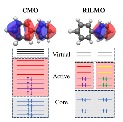
Figure 1: Example of fragmentation and definiton of the fragment active spaces. (Left) Active space selection for the entire biphenyl molecule. The CAS treatment separates the canonical molecular orbitals (CMOs) based on their energy ordering, obtaining a set of doubly-occupied core orbitals, a set of empty virtual orbitals, and a set of active orbitals around Fermi energy used to describe correlations. We illustrate the highest occupied molecular orbital. (Right) Fragment active space selection for the left and right fragments of the biphenly molecule. After the localization procedure, we obtain Recanonicalized Intrinsic Localized Molecular Orbitals (RILMOs), where the orbitals are assigned to either fragment A or B. We can still select core, active and virtual orbitals for each fragment based on an approximate energy ordering, obtained through the recanonicalization procedure. Here we depict the highest occupied RILMO for the right fragment. Using our method, we can half the size of the required active space since the multi-reference solver is applied to just one fragment at a time. The correlations between the localized active spaces can be retrieved afterwards with perturbation theory.

II FragPT2 method

In this section, we introduce a novel method for fragmented multi-reference calculations with perturbative corrections: FragPT2. This method works by dividing the active space of a molecule into localized subspaces that can be treated separately using a MC solver, as illustrated in Figure 1. The cost of MC methods scales quickly with the size of the treated active space (e.g. exponentially in the case of FCI); splitting the system into smaller active spaces allows the treatment of larger systems for an affordable computational cost. In this work, we focus on the special case of two active fragments called $A$ and $B$; however, our method can be promptly generalized to the multiple fragment case as discussed in Section IV.3. Our method requires the user to define the molecular fragments as an input. The choice of fragmentation should be based on chemical intuition, aiming at minimizing inter-fragment correlations; a good choice is crucial to the success of the method. Our method allows to recover some inter-fragment correlations, allowing fragmentations that break a covalent bond (like the one shown in Figure 1 for biphenyl), i.e. where two atoms on either side of a covalent bond are assigned to different fragments. The number of bonds broken in fragmentation should, however, be kept to a minimum.

First, in Sec II.1 we introduce the construction of the localized orbitals and the definition of the fragment active spaces. In Section II.2 we define fragment Hamiltonians by embedding each fragment in the mean field of the other. Applying separate MC solvers to each fragment Hamiltonian, we show how to obtain a fragment product state $\ket{\Psi_{0}}$ which will be the reference state for subsequent perturbative expansions. Finally, in Section II.3 we decompose the full Hamiltonian into a sum of the solved fragment Hamiltonians and a number of inter-fragment interaction terms. We classify these terms on the basis of fragment symmetries and describe a method to treat them in second-order perturbation theory.

II.1 Construction of re-canonicalized intrinsic localized molecular orbitals

In order to define the fragment subspaces, we follow the top-down procedure introduced in [46], based on localizing pre-computed molecular orbitals. First, we calculate a set of canonical molecular orbitals (CMOs) for the whole system (other choices for molecular orbitals are discussed in Section IV). At this stage we also choose a valence space, freezing a set of hard-core and hard-virtual orbitals far from Fermi energy. Distinct Hartree-Fock calculations are also run on each fragment, removing all nuclei and electrons in the other; these result in the definition of two sets of reference fragment orbitals (RFOs). The RFOs from fragment A are not orthogonal to the ones from fragment B. To deal with this, the RFOs from both fragments are projected to the space spanned by the CMOs [47]. This yields an orthonormal set of intrinsic fragment orbitals (IFOs) expressed in the CMO basis, each assigned to one fragment but without a clear energy ordering. In the final step, the CMOs are localized in the IFO basis of either fragment, using a Pipek-Mezey localization scheme [48]; the occupied orbitals and empty orbitals within the active space are localized separately. This procedure results in a set of Recanonicalized Intrinsic Localized Molecular Orbitals (RILMOs), partitioned in two fragment subspaces, that together span the same space defined by the original CMOs. An approximate energy ordering for the RILMOs is obtained by block-diagonalizing the Fock matrix within each fragment. The active spaces for each fragment (illustrated in Figure 1) are defined by choosing a set of RILMOs around Fermi energy.

We adapt this localizion scheme to work for covalently bonded fragments, where there is an ambiguity in assigning one occupied orbital representing the bond to either fragment. To eliminate this arbitrariness, we introduce a bias so that any such bond is always assigned to the first fragment. This enables us to define a natural fragmentation for covalently bonded dimer molecules. To generate the required IFO basis for this calculation, we cut through the single covalent bond and cap the dangling bonds with hydrogen atoms. This method proves to be simple and efficient, though it necessitates caution as it introduces an additional orbital in the span of the IFOs. We find this strategy works well for the covalently bonded dimer systems tested in this work.

II.2 Fragment embedding

The total Hamiltonian in the combined active space spanned by both fragments is given by

$$H=\sum_{pq\in A\cup B}h_{pq}E_{pq}+\frac{1}{2}\sum_{pqrs\in A\cup B}g_{pqrs}e_{pqrs},$$ (1)

where we use the spin-adapted excitation operators

$$E_{pq} =\sum_{\sigma}a_{p\sigma}^{\dagger}a_{q\sigma},$$ (2)

$$e_{pqrs} =\sum_{\sigma\tau}a_{p\sigma}^{\dagger}a_{r\tau}^{\dagger}a_{s\tau}a_{q\sigma}=E_{pq}E_{rs}-\delta_{qr}E_{ps}.$$

This Hamiltonian includes all interactions of all active orbitals. Our embedding scheme aims at decomposing this Hamiltonian as $H=H^{0}+H^{\prime}$, where $H^{0}$ includes intra-fragment terms and a mean-field inter-fragment term, and can be solved exactly with separate in-fragment MC solvers. The residual inter-fragment interactions $H^{\prime}$ are treated separately with perturbation theory, as described in Section II.3.

To facilitate the use of separate MC solvers for each fragment, we constrain the wavefunction of the total system to be a product state over the two fragments,

$$\ket{\Psi^{0}}=\ket{\Psi_{A}}\ket{\Psi_{B}},$$ (3)

where $\ket{\Psi_{X}}$ is a many-body wavefunction in the active space of fragment $X$. We further restrict each fragment wavefunction $\ket{\Psi_{X}}$ to have fixed, integer charge and spin. Note that the conservation of spin and charge on each fragment is not a symmetry of the subsystem; however, this assumption is crucial to construct separate efficient MC solvers. Inter-fragment charge transfer and spin exchange processes are later treated in perturbation theory.

Under these constraints, we can simplify the expression of $H$ by removing all the terms that do not respect charge and spin conservation on each fragment separately (as their expectation value of $\ket{\Psi^{0}}$ would anyway be zero). The remaining Hamiltonian can be then decomposed as $H_{A}+H_{B}+H_{AB}$, with terms

$$H_{X}=\sum_{pq\in X}h_{pq}E_{pq}+\frac{1}{2}\sum_{pqrs\in X}g_{pqrs}e_{pqrs}$$ (4)

(with $X\in\{A,B\}$), that only act non-trivially on a single fragment, and a term

$$H_{AB}=\sum_{pq\in A}\sum_{rs\in B}g^{\prime}_{pqrs}E_{pq}E_{rs}$$ (5)

(where $g^{\prime}_{pqrs}=g_{pqrs}-\frac{1}{2}g_{psrq}$), that includes interactions preserving local spin and charge. The term $H_{AB}$ still introduces inter-fragment correlations; one way to make the fragments completely independent would be to also treat this term perturbatively (this is the choice made in SAPT [38]). However, including an effective mean-field interaction (originating from $H_{AB}$) in the non-perturbative solution improves the quality of our $\ket{\Psi^{0}}$.

To construct the effective Hamiltonian $H^{\text{eff}}_{X}$ for each fragment we use a mean-field decoupling approach. We write the excitation operator as its mean added to a variation upon the mean: $E_{pq}=\expectationvalue{E_{pq}}+\delta E_{pq}$. The mean is just the one-particle reduced density matrix (1-RDM) of one of the fragments, $\gamma^{X}_{pq}=\matrixelement{\Psi_{X}}{E_{pq}}{\Psi_{X}}$. By substituting in Eq. (5) we obtain

$$\sum_{pq\in A}\sum_{rs\in B}g^{\prime}_{pqrs}\left[E_{pq}\gamma^{B}_{rs}+\gamma^{A}_{pq}E_{rs}-\gamma^{A}_{pq}\gamma^{B}_{rs}+\delta E_{pq}\delta E_{rs}\right].$$ (6)

The term $\delta E_{pq}\delta E_{rs}$ will necessarily have zero expectation value on the product state Eq. (3), as $\expectationvalue{\delta E_{pq}}{\Psi_{X}}=0$. Removing this term (which we will later treat perturbatively) we obtain the mean-field interaction

$$H_{\text{mf}}=\sum_{pq\in A}\sum_{rs\in B}g^{\prime}_{pqrs}\left[E_{pq}\gamma^{B}_{rs}+\gamma^{A}_{pq}E_{rs}-\gamma^{A}_{pq}\gamma^{B}_{rs}\right].$$ (7)

We can finally define $H^{0}$ as

$$H^{0} =H_{A}+H_{B}+H_{\text{mf}},$$ (8)

where all terms are operators with support on only a single fragment, thus the ground state $\ket{\Psi^{0}}$ of $H^{0}$ is a product state of the form Eq. (3). All the terms we removed from $H$ to construct $H^{0}$ have zero expectation value on $\ket{\Psi^{0}}$, thus it is the lowest energy product state that respects the on-fragment symmetries.

To find $\ket{\Psi^{0}}$ we minimize $E_{0}=\expectationvalue{H^{0}}$ by self-consistently solving separate ground state problems on each fragment. Consider the decomposition

$$E_{0} =E_{A}+E_{B}+C^{\rm eff},$$ (9)

where $E_{X}=\matrixelement{\Psi_{X}}{H_{X}}{\Psi_{X}}$ can be evaluated on a single fragment $X$ and $C^{\rm eff}=\sum_{pq\in A}\sum_{rs\in B}g^{\prime}_{pqrs}\gamma^{A}_{pq}\gamma^{B}_{rs}$ is a constant depending on the fragment 1-RDMs. To find $\ket{\Psi_{A}}$ and $\ket{\Psi_{B}}$, we iteratively solve for the ground state of the following coupled Hamiltonians:

$$H^{\rm eff}_{A} =H_{A}+\sum_{pq\in A}\sum_{rs\in B}g^{\prime}_{pqrs}E_{pq}\gamma^{B}_{rs}$$ (10)

$$H^{\rm eff}_{B} =H_{B}+\sum_{pq\in A}\sum_{rs\in B}g^{\prime}_{pqrs}\gamma^{A}_{pq}E_{rs},$$ (11)

thus minimizing all the terms Eq. (9). We outline the whole procedure in Algorithm 1.

Input: Active space integrals $h_{pq}$, $g_{pqrs}$. Fragment-partitioned sets of orbitals: occupied $(O_{\text{A}},O_{\text{B}})$, and virtual $(V_{\text{A}},V_{\text{B}})$ subspaces. Convergence threshold $\tau$.

Output: Optimal product state $\ket{\Psi^{0}}=\ket{\Psi_{A}}\ket{\Psi_{B}}$

Start from a Hartree-Fock state: $\gamma^{B}_{pq}\leftarrow 2\delta_{pq}$ for $p,q\in O_{B}$;

$\Delta E,\,E^{0}\leftarrow\infty$;

while  $\Delta E>\tau$ do

       $\ket{\Psi_{A}},E^{\rm eff}_{A}\leftarrow$ ground state of $H^{\rm eff}_{A}$ of Eq. (10) ;

       $\gamma^{A}_{pq}\leftarrow\matrixelement{\Psi_{A}}{E_{pq}}{\Psi_{A}}$, $p,q\in A$;

       $\ket{\Psi_{B}},E^{\rm eff}_{B}\leftarrow$ ground state of $H^{\rm eff}_{B}$ of Eq. (11);

       $\gamma^{B}_{rs}\leftarrow\matrixelement{\Psi_{B}}{E_{rs}}{\Psi_{B}}$, $p,q\in B$;

       $C^{\rm eff}\leftarrow\sum_{pq\in A}\sum_{rs\in B}g^{\prime}_{pqrs}\gamma^{A}_{pq}\gamma^{B}_{rs}$;

       $\Delta E\leftarrow E^{0}-(E^{\rm eff}_{A}+E^{\rm eff}_{B}-C^{\rm eff})$;

       $E^{0}\leftarrow(E^{\rm eff}_{A}+E^{\rm eff}_{B}-C^{\rm eff})$

return $\ket{\Psi^{0}}=\ket{\Psi_{A}}\ket{\Psi_{B}}$

Algorithm 1 Fragment embedding

	Perturbation	Perturbing functions $\left\{\ket{\Psi_{\mu\nu}}\right\}$	Fragment matrix element
1.	${\begin{aligned} H^{\prime}_{\rm disp}=&\sum_{pq\in A}\sum_{rs\in B}g^{\prime}_{pqrs}\left(E_{pq}-\gamma^{A}_{pq}\right)\left(E_{rs}-\gamma^{B}_{rs}\right)\end{aligned}}$	${\begin{aligned} E&{}_{tu}E_{vw}\ket{\Psi^{0}}\\ &\begin{bmatrix}tu\in A,\,vw\in B\end{bmatrix}\end{aligned}}$	${\matrixelement{\Psi_{X}}{E_{lk}H^{\rm eff}_{X}E_{tu}}{\Psi_{X}}}$
2.	${\begin{aligned} H^{\prime}_{\rm 1CT}=&\sum_{p\in A}\sum_{q\in B}\left[h_{pq}-\sum_{r\in A}g_{prrq}\right]E_{pq}\\ &+\sum_{p\in B}\sum_{q\in A}\left[h_{pq}-\sum_{r\in B}g_{prrq}\right]E_{pq}\\ &+\sum_{pqr\in A}\sum_{s\in B}g_{pqrs}E_{pq}\left[E_{rs}+E_{sr}\right]\\ &+\sum_{pqr\in B}\sum_{s\in A}g_{pqrs}E_{pq}\left[E_{rs}+E_{sr}\right]\end{aligned}}$	${\begin{aligned} E&{}_{tu}E_{vw}\ket{\Psi^{0}}\\ &\begin{bmatrix}tuv\in A,w\in B\\ tuw\in A,v\in B\\ tuv\in B,w\in A\\ tuw\in B,v\in A\end{bmatrix}\end{aligned}}$	${\begin{aligned} \matrixelement{\Psi_{X}}{a_{m}E_{lk}H^{\rm eff}_{X}E_{tu}a^{\dagger}_{v}}{\Psi_{X}}\\ \matrixelement{\Psi_{X}}{a^{\dagger}_{m}E_{lk}H^{\rm eff}_{X}E_{tu}a_{v}}{\Psi_{X}}\end{aligned}}$
3.	${\begin{aligned} H^{\prime}_{\rm 2CT}=&\frac{1}{2}\sum_{pr\in A}\sum_{qs\in B}g_{pqrs}E_{pq}E_{rs}\\ &+\frac{1}{2}\sum_{pr\in B}\sum_{qs\in A}g_{pqrs}E_{pq}E_{rs}\end{aligned}}$	${\begin{aligned} E&{}_{tu}E_{vw}\ket{\Psi^{0}}\\ &\begin{bmatrix}tv\in A,uw\in B\\ uw\in A,tv\in B\\ \end{bmatrix}\end{aligned}}$	${\begin{aligned} \matrixelement{\Psi_{X}}{a_{l}a_{k}H^{\rm eff}_{X}a^{\dagger}_{t}a^{\dagger}_{u}}{\Psi_{X}}\\ \matrixelement{\Psi_{X}}{a^{\dagger}_{l}a^{\dagger}_{k}H^{\rm eff}_{X}a_{t}a_{u}}{\Psi_{X}}\end{aligned}}$
4.	${\begin{aligned} H^{\prime}_{\rm TT}=-\sum_{pq\in A}\sum_{rs\in B}g_{psrq}t_{pq,rs}\end{aligned}}$	${\begin{aligned} &t_{tu,vw}\ket{\Psi^{0}}\\ &\begin{bmatrix}tu\in A,\,vw\in B\end{bmatrix}\end{aligned}}$	${\begin{aligned} &\matrixelement{\Psi_{X}}{T^{(1,0)}_{lk}H^{\rm eff}_{X}T^{(1,0)}_{tu}}{\Psi_{X}}\\ &\matrixelement{\Psi_{X}}{T^{(1,1)}_{lk}H^{\rm eff}_{X}T^{(1,-1)}_{tu}}{\Psi_{X}}\\ &\matrixelement{\Psi_{X}}{T^{(1,-1)}_{lk}H^{\rm eff}_{X}T^{(1,1)}_{tu}}{\Psi_{X}}\end{aligned}}$

Table 1: Summary of the perturbations and the cost of PT2. We summarize here the perturbing functions and cost for each of the perturbations. The rightmost column reports the form of the matrix elements of $H^{0}$ required to compute each perturbation; estimating these matrix elements on the fragment state is the most expensive part of FragPT2. If done naively by writing out the full fragment Hamiltonians as a contraction between integrals and this could require estimating 4-RDMs for the dispersion, double charge transfer (2CT) and triplet-triplet (TT) perturbations, and 5-RDMs for the single charge transfer (1CT) perturbation.

II.3 Multi-reference perturbation theory

While the $\ket{\Psi^{0}}$ retrieved from Algorithm 1 is a solid starting point, it neglects the correlations between the fragments. If the fragments are sufficiently separated, we expect these correlations to be minimal and recoverable by perturbation theory. We propose using second-order perturbation theory to retrieve the correlation energy of these interactions. The inter-fragment interaction terms can be classified in four categories, based on whether they conserve charge and/or total spin on each fragment: dispersion $H^{\prime}_{\text{disp}}$ (which conserves both charge and spin of the fragments), single-charge transfer $H^{\prime}_{\text{1CT}}$ and double-charge transfer $H^{\prime}_{\text{2CT}}$ (that conserve charge nor spin), and triplet-triplet coupling $H^{\prime}_{\text{TT}}$ (that conserves charge but not local spin). Thus, the complete decomposition of the Hamiltonian reads:

$$H=H^{0}+H^{\prime}_{\rm disp}+H^{\prime}_{\rm 1CT}+H^{\prime}_{\rm 2CT}+H^{\prime}_{\rm TT}.$$ (12)

The definition of these terms is given in Table 1 and their derivation is reported in Appendix A. We will treat the different perturbations in Eq. (12) one at a time. First notice that for every perturbation in Eq. (12), the first order energy correction is zero: $E^{1}=\matrixelement{\Psi^{0}}{H^{\prime}}{\Psi^{0}}=0$. We will focus solely on the second order correction to the energy.

To proceed, we need to choose a basis of perturbing functions $\left\{\ket{\Psi_{\mu}}\right\}$ used to define the first-order correction to the wavefunction

$$\ket{\Psi^{1}}=\sum_{\mu}C_{\mu}\ket{\Psi_{\mu}}.$$ (13)

For the exact second order perturbation energy, we should consider all Slater determinants that can be obtained by applying the terms within $H$ to the set of reference determinants. While this full space of perturbing functions is smaller than the complete eigenbasis of $H$, it is still unpractically large, and approximations need to be introduced. To choose a compact and expressive basis, we look at the perturbation under consideration. Every perturbative Hamiltonian can be expanded in a linear combination of two-body operators:

$$H^{\prime}=\sum_{\mu\in A}\sum_{\nu\in B}g_{\mu\nu}O^{A}_{\mu}O^{B}_{\nu}.$$ (14)

where $O^{X}_{\mu}$ is either identity or a product of Fermionic operators on fragment $X$ and $g_{\mu\nu}$ are combinations of one- and two-electron integrals (see Table 1 for their explicit form). Consider the following (non-orthogonal) basis:

$$\ket{\Psi_{\mu\nu}}=O^{A}_{\mu}O^{B}_{\nu}\ket{\Psi^{0}}.$$ (15)

This is a natural choice for the perturbing functions that compactly represents wavefunctions that interact with $\ket{\Psi^{0}}$ through the perturbation.

Following the choice of perturbing functions, we estimate the matrix elements $\matrixelement{\Psi_{\mu\nu}}{H^{0}}{\Psi_{\kappa\lambda}}$ in this basis. The overlap $\bra{\Psi_{\mu\nu}}\ket{\Psi_{\kappa\lambda}}$ must also be computed in order to be able to contract with the $g_{\mu\nu}$ to yield $\matrixelement{\Psi^{0}}{H^{\prime}}{\Psi_{\mu\nu}}$. To obtain the coefficients $C_{\mu\nu}$ that define the first-order correction to the wavefunction, we solve the following linear equations:

$$\sum_{\kappa\lambda}\matrixelement{\Psi_{\mu\nu}}{H^{0}-E^{0}}{\Psi_{\kappa\lambda}}C_{\kappa\lambda}+\matrixelement{\Psi_{\mu\nu}}{H^{\prime}}{\Psi^{0}}=0.$$ (16)

Then the second-order correction to the energy is given by:

$$E^{2}=\matrixelement{\Psi^{0}}{H^{\prime}}{\Psi^{1}}=\sum_{\mu\nu}\matrixelement{\Psi^{0}}{H^{\prime}}{\Psi_{\mu\nu}}C_{\mu\nu}.$$ (17)

The algorithm is summarized in Algorithm 2.

Input: Active space integrals and orbital partitioning as in Algorithm 1. Zeroth-order product state $\ket{\Psi^{0}}=\ket{\Psi_{A}}\ket{\Psi_{B}}$.

Output: Second-order perturbative corrections: $E^{2}_{\rm disp},\,E^{2}_{\rm 1CT},\,E^{2}_{\rm 2CT}$ and $E^{2}_{\rm TT}$

for $H^{\prime}\in\{H^{\prime}_{\rm disp},\,H^{\prime}_{\rm 1CT},\,H^{\prime}_{\rm 2CT},\,H^{\prime}_{\rm TT}\}$ do

       Choose perturbing functions as in Eq. (15);

       Compute matrix elements $\matrixelement{\Psi_{\mu\nu}}{H^{0}}{\Psi_{\kappa\lambda}}$;

       Compute matrix elements $\matrixelement{\Psi_{\mu\nu}}{H^{\prime}}{\Psi^{0}}$;

       $C_{\mu\nu}\leftarrow$ solution of Eq. (16);

       $E^{2}\leftarrow\sum_{\mu\nu}\matrixelement{\Psi^{0}}{H^{\prime}}{\Psi_{\mu\nu}}C_{\mu\nu}$

return $E^{2}_{\rm disp},\,E^{2}_{\rm 1CT},\,E^{2}_{\rm 2CT}$ and $E^{2}_{\rm TT}$

Algorithm 2 FragPT2

Computing the matrix elements $\matrixelement{\Psi_{\mu\nu}}{H^{0}}{\Psi_{\kappa\lambda}}$ is the most expensive part of our algorithm. The tensor product form of the zeroth-order wavefunction significantly reduces the algorithm’s cost by allowing the matrices to factorize in the expectation values of operators on the different fragments, that in turn can be expressed as combinations of fragment RDMs. We outline the idea here, and refer the reader to Appendix B for the formal derivation for every perturbation:

$$\matrixelement{\Psi_{\mu\nu}}{H^{0}}{\Psi_{\kappa\lambda}} =$$ (18)

$$\matrixelement{\Psi_{A}}{{O^{A}_{\mu}}^{\dagger}H^{\rm eff}_{A}O^{A}_{\kappa}}{\Psi_{A}}\matrixelement{\Psi_{B}}{{O^{B}_{\nu}}^{\dagger}O^{B}_{\lambda}}{\Psi_{B}}$$

$$+ \matrixelement{\Psi_{A}}{{O^{A}_{\mu}}^{\dagger}O^{A}_{\kappa}}{\Psi_{A}}\matrixelement{\Psi_{B}}{{O^{B}_{\nu}}^{\dagger}H^{\rm eff}_{B}O^{B}_{\lambda}}{\Psi_{B}}$$

$$+ C^{\rm eff}\matrixelement{\Psi_{A}}{{O^{A}_{\mu}}^{\dagger}O^{A}_{\kappa}}{\Psi_{A}}\matrixelement{\Psi_{B}}{{O^{B}_{\nu}}^{\dagger}O^{B}_{\lambda}}{\Psi_{B}}.$$

If there are $N_{A}N_{B}$ two-body terms in Eq. (14), the number of matrix elements that one needs to estimate on each fragment is $\frac{1}{2}N_{A}N_{B}(N_{A}N_{B}+1)$. However, if the amount of matrix elements becomes too expensive, it is possible to alleviate the cost without sacrificing much accuracy by using contracted versions of the basis of perturbing functions, a popular method in CASPT2 and NEVPT2 [35]. For a discussion of further reductions of the cost, see Section IV.1.

III Numerical demonstration

In this section we demonstrate our method by applying it to a range of molecular systems that are well-suited targets for bipartite fragmentation. We have chosen three sets of systems. The first system consists of two N2 molecules at a distance of $2.0$\mathrm{\text{Å}}$$, with a (close to equilibrium) bond length of $1.2$\mathrm{\text{Å}}$$. In contrast to the other structures, we do not need to cut through a covalent bond and can treat each molecule as a separate fragment. We examine the results of our method while stretching the nitrogen bond in one of the fragments; this is known to rapidly increase static correlation in this system and thus is a good benchmark for the multi-reference method. The second type of systems we consider comprises a set of aromatic dimers, where two aromatic rings of different kinds are connected by a single covalent bond. Cutting through this bond, we investigate the correlation energies of the dimers with respect to the dihedral angle of the ring alignment. These systems exhibit strong correlation whenever the rings are in the same plane and low correlation when the rings are perpendicular to each other: they are thereby suitable to benchmark both regimes. The final system is butadiene, as the simplest example of the class of polyene molecules that are much studied as 1-D model systems [49, 50] as well as for their importance in various applications [51, 52, 53]. Here we cut through the single covalent bond between the middle carbons and investigate the correlation energy with respect to the stretching of the double bonds in a single fragment. This system, albeit slightly artificial, is intriguing due to the significant static correlation within the fragments induced by the dissociating bonds, coupled with substantial dynamic inter-fragment correlation.

III.1 Numerical simulation details

We construct the localized orbitals using a localization scheme implemented in the ROSE code [54]. The FragPT2 method is implemented completely inside the quantum chemical open-source software package PySCF [55]. Algorithm 1 uses the FCI solver of the program to get the optimal product state of the fragments. The matrix elements in Eq. (18) by exploiting the software capabilities to manipulate CI-vectors and estimate higher order RDMs. Finally we implemented Algorithm 2 that solves Eq. (16) and (17) for every perturbation in Eq. (12). To assess the accuracy of our algorithm, we compare the fragment embedding energy $E^{0}$ (from Algorithm 1), the FragPT2 energy $E^{0}+E^{2}$ including the perturbative correction (from Algorithm (17)), and the exact ground state energy $E^{\rm exact}$ of the Hamiltonian in Eq. (1) (calculated with CASCI in an a full-molecule active space of dobule size). The N2 dimer and aromatic dimer calculations are done in a cc-pVDZ basis set, while butadiene is treated in a 6-31G basis.

III.2 N2 dimer

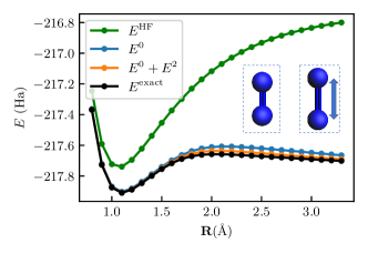
Figure 2: Potential energy curve for the N2 dimer. Comparison of the curves obtained through Hartree-Fock ($E^{\text{HF}}$), fragment embedding ($E^{0}$), FragPT2 ($E^{0}+E^{2}$), and full-molecule CASCI (exact). The two N2 are parallel and at a distance of $\mathrm{2}\mathrm{\text{Å}}$ (geometry shown in the inset). The curve shows the energy as a function the bond distance of one of the N2. The fragment active spaces each comprise six electrons in six spatial orbitals, corresponding to the triple bonding and anti-bonding orbitals. Hartree-Fock performs poorly due to the strong intra-frament correlation. The fragment embedding energy $E^{0}$ captures the correct behaviour of the system, while $E^{2}$ gives an additional, small correction in the direction of the exact solution.

As an initial test system, we consider a dimer of nitrogen molecules, i.e. N2-N2. To increase the static correlation within the fragment, we dissociate one of the nitrogen molecules. This bond breaking is modeled using three occupied and three virtual localized orbitals in the active space, representing the $\sigma$ bond and the two $\pi$ bonds. This results in an active space of six electrons in six orbitals for each fragment. The results in Figure 2 clearly demonstrate the failure of the Hartree-Fock method due to the high degree of correlation within the fragment. Our multi-reference solver within the localized active spaces successfully addresses this issue, with $E^{0}$ providing a good description of the ground state. There is some minor inter-fragment correlation, and our perturbative correction brings us closer to the exact solution.

Our data further shows that the perturbative correction arises only from the single-charge transfer contribution, and other corrections are negligible. In particular, we find that the dispersion interaction between the fragments is minimal. The ability to identify the character of the relevant interactions between fragments is a further advantage of our method.

III.3 Aromatic dimers

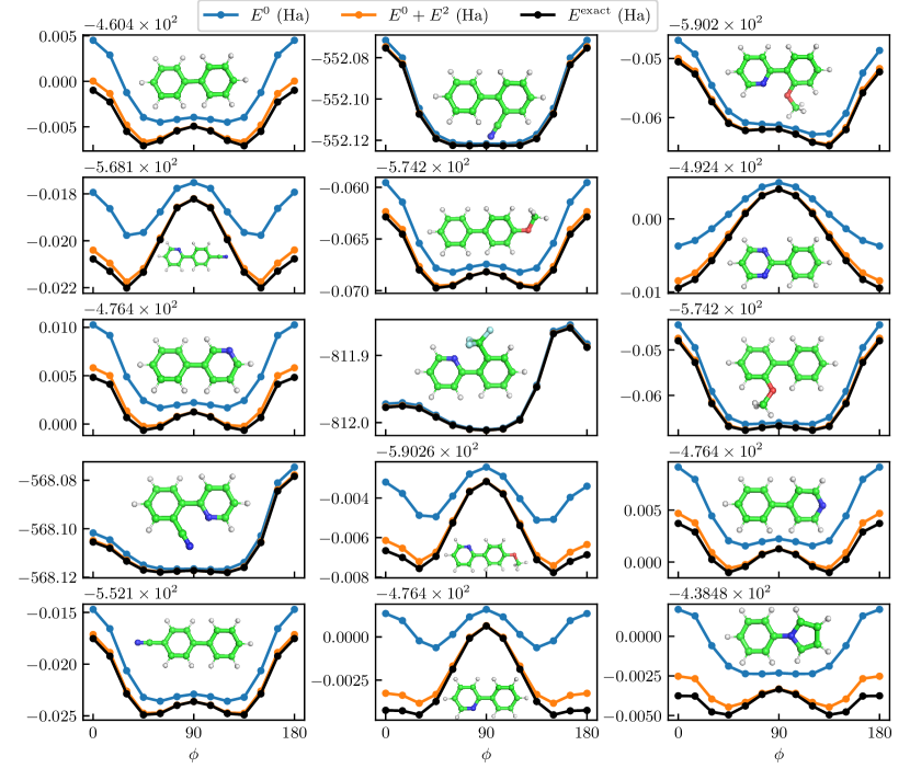
Figure 3: Potential energy curves for the set of aromatic dimers, where we vary the dihedral angle $\phi$ of the two dimers. The molecular orbitals are localized on the fragments naturally defined by the two aromatic rings (including the respective ligands). In principle, for each dimer, we select the active space of six electrons in six orbitals on each fragment that comprise the conjugated $\pi-\pi^{*}$ system (with some exceptions elaborated on in Section III.3). Thus our method cuts down the space for the exact calculation (twelve electrons in twelve orbitals) into half. This is small enough to verify our method against an exact CASCI calculation. The blue line represents the fragment embedding energy $E^{0}$. The orange line includes the second-order perturbation energy for all considered perturbations, representing the FragPT2 energy $E^{0}+E^{2}$. The black line reports the exact calculation $E^{\rm exact}$. The considered molecules are, in row-first order: (a) biphenyl (b) 2-cyanobiphenyl (c) 2-(2-methoxyphenyl)pyridine (d) 2-(4-cyanophenyl)pyridine (e) 4-methoxybiphenyl (f) 2-phenylpyrimidine (g) 3-phenylpyridine (h) 2-(2-trifluoromethylphenyl)pyridine (i) 2-methoxybiphenyl (j) 2-(2-cyanophenyl)pyridine (k) 2-(4-methoxyphenyl)pyridine (l) 4-phenylpyridine (m)4-cyanobiphenyl (n) 2-phenylpyridine (o) N-phenylpyrrole.

Here we focus on aromatic dimers, i.e. molecules with two aromatic rings that are attached by a single covalent bond. The simplest such system considered is two phenyl rings, known as biphenyl, shown in Figure 1. As the biphenyl case is highly symmetric, other similar molecules can be generated by substituting various ligands for one of the hydrogen atoms, or a nitrogen for a carbon in the phenyl rings. In this manner, we generate a comprehensive benchmark on a variety of systems. Our set of examples is motivated from the different classes of biaryl systems studied by Sanfeliciano et al. in the context of drug design [56].

To construct the fragment active spaces, we consider the conjugated $\pi-\pi^{*}$ system on each ring, typically resulting in six electrons distributed across six orbitals for each fragment. There are a few exceptions to this rule. For pyrrole rings, the relevant aromatic orbitals comprise six electrons in five orbitals. Furthermore, for rings that include a CN or OCH3 substituent [i.e. (c-f), (i-k) and (m) in Figure 3], there is a low-lying $\pi$ orbital and high-lying $\pi^{*}$ orbital that mix with a $p$ orbital of the substituent. These orbitals are excluded from the active space of these fragments, reducing the active space to four electrons in four orbitals. This only provides additional insight into the performance of our method with asymmetric active space sizes in the fragments.

For each dimer, we vary the dihedral angle $\phi$ of the two planes spanned by the rings, thus rotating over the covalent bond. This gives a potential energy curve with a high variance of correlation energy: if the rings are perpendicular, the aromatic systems are localized and the correlation between the fragments is low. Instead, if the rings are aligned, we expect to see a high amount of correlation between the fragments, and thus a breakdown of the description of $E^{0}$. The results of our method compared to the exact energies are given in Figure 3.

Figure 4: Average errors for the aromatic dimer set. Mean Absolute Deviation in total energy with respect to the exact result for the complete set of aromatic dimers shown in Figure 3, where we vary the dihedral angle $\phi$ of the two aromatic rings. We show the result of sequentially adding the different perturbative corrections described in Tab. 1. The top curve represents the error of fragment embedding energy $E^{0}$. To this, we first add the dispersion correction $E^{2}_{\text{disp}}$, which is giving a constant shift along the dihedral angle. Then, the (single) charge transfer correction $E^{2}_{\text{1CT}}$ crucially corrects for the behaviour where the rings are aligned. Finally, we add the double charge transfer term $E^{2}_{\text{2CT}}$ and triplet-triplet term $E^{2}_{\text{TT}}$ together, recovering the final FragPT2 energy $E^{0}+E^{2}$. These last terms contribute an additional small shift to the aligned rings configuration.

For each of the molecules and values of $\phi$, $E^{0}$ recovers at least $93\%$ of the correlation energy (with an average of $97\%$). While this is high in absolute terms, the shape of the potential energy curves for these models can be qualitatively wrong. As expected, a product state is not a good approximation if the rings are aligned, as the aromatic system will be delocalized over the molecule. This causes the interactions between the fragments to play a more significant role. The product state is on the other hand a good approximation when the rings are perpendicular, there pushing $E^{0}$ to $99\%$ of the correlation energy. This causes an imbalance between the two configurations and calls for the need to treat the interactions. When we compute the second-order perturbation energy $E^{2}$, it is shown in Figure 3 that sometimes $E^{0}$ finds a different minimum than the exact state. In these cases especially, the perturbative corrections need to be calculated to give a more correct shape of the potential energy curve. In Figure 4, one can see that the division of the perturbation energies can be very constructive in determining the important contributions of the system in question. In case of aromatic dimers, two interactions are important: dispersion and single-charge transfer. While the former takes care of a constant shift over the dihedral angles, the latter is much larger when the aromatic rings are aligned, thus crucial in retrieving the right behaviour of PES. The double-charge transfer and triplet-triplet spin exchange terms are not important in these class of molecules.

III.4 Butadiene

Butadiene (C4H6) is the final test system that we consider. We define the two fragments by cutting through the middle bond of the molecule. We study the energy of the system while stretch the double bond onto dissociation inside one of the fragments, thereby testing our method to increasing amounts of static correlation inside the fragment. Dissociating the bond additionally causes the leftover molecule to be a radical, thus increasing significantly the strength of the interaction between the fragments.

We define the active spaces by taking the $\pi-\pi^{*}$ and $\sigma-\sigma^{*}$ system of the double bonds of both fragments. This results in an active space of four electrons in four orbitals for each fragment.

The potential energy curves are shown in Figure 5. It can be clearly seen that the multi-reference product state is a correct description at the equilibrium geometry, but its performance is somewhere in between the Hartree-Fock and the exact solution at dissociation. To improve on it, we clearly need the perturbative corrections. If we analyze the contributions to the perturbative correction, we see that $H^{\prime}_{\rm 1CT}$ interaction is the most important (contributing around $80\sim 88\%$ to $E^{2}$). Notably, in this system the $H^{\prime}_{\rm TT}$ contribution is large as well (contributing around $8\sim 12\%$ to $E^{2}$). This is in line with chemical intuition, as this system has low-lying triplet states [57]; a singlet-coupled double triplet excitation may therefore contribute significantly to the ground state wave function. Again, the ability to separately analyze the different classes of inter-fragment interactions is useful here, as it allows to consider the correlation in polyenes in terms of products of local excitations.

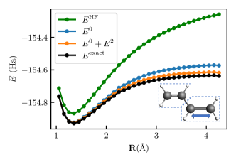
Figure 5: Potential energy curves of butadiene. The fragments are chosen by cutting through the middle bond and subsequently stretching the double bond of one of the fragments, as illustrated in the inset. The curves are color coded like in Figure 2, and show that both intra-fragment and inter-fragment correlations are important to recover the correct behavior. In particular, inter-fragment correlations are explained by the vicinity of the two fragments and by the radical that is left over after dissociation of the stretched bond.

IV Conclusion and outlook

In this work, we introduced a novel multi-reference multi-fragment embedding framework called FragPT2. We show that our method gives accurate results for a reduced cost in active space size, especially when fragments are well separated. Our comprehensive numerical benchmarks on a variety of molecules show that: 1. Intra-fragment static correlation can be retrieved by an MC product state ansatz ($E^{0}$) 2. Inter-fragment correlation can be treated as a perturbative correction ($E^{2}$) 3. A combination of these is needed to recover the correct shape of the potential energy curve. Using the decomposition of the Hamiltonian, we can distinguish the contributions to the inter-fragment correlation in $E^{2}$, providing insight into important interactions within the studied systems. Thanks to our adapted localization scheme we can define molecular fragments that cut through covalent bonds. In this case, perturbative corrections describing inter-fragment charge transfer (and, to a lesser extent, triplet-triplet spin exchange) are crucial for accurately describing the system.

Our multi-reference embedding scheme could find broad applications, for instance in understanding the spatial dependence of the correlation energy in $\pi$-stacked systems and other biochemically important systems [58], modelling supramolecular complex formation [59] in metal ion separation, or in analyzing metallophylic interactions [60, 61, 62].

IV.1 Computational efficiency

Upon working out the $H^{0}$ matrix elements in Eq. (18) for the different perturbations, one ends up with k-order RDMs where k goes up to 4 or even 5. Evaluating these RDMs naively requires the storage of up to 8 or 10 index tensors which is computationally expensive. There exists several methods which bypasses the explicit storage and construction of such tensors and has been proposed in literature in the context of NEVPT2. Resolution of identity (RI) [63], cumulant expansions [64], tensor contraction with integrals [65, 66] are some of the ways to circumvent this bottleneck. A recent work by Neese and co-workers [67] explored different approximations to the higher-order RDMs encountered in the partially contracted version of NEVPT2 using some of these above techniques [67, 68]. Strongly contracted versions of our algorithm can also be devised. One way forward is to apply directly the perturbation to $\ket{\Psi^{0}}$ as a single perturbing function. The bottleneck of the algorithm then becomes estimating higher order powers of the Hamiltonian and the perturbations on $\ket{\Psi^{0}}$, effectively equivalent to the first order of a moment expansion [69, 35]. Another way of relieving the cost are stochastic formulations of MRPT, presented separately by Sharma et al [70, 71] and Booth et al [72] in the context of strongly-contracted NEVPT2, wherein the necessary quantities were determined in a quantum Monte-Carlo (QMC) framework.

IV.2 Integration with quantum algorithms

In this manuscript we focused on solving the single fragments with FCI, however our framework is compatible with any method that allows to recover reduced density matrices of the fragment wavefunctions. The last decade has seen the emergence of quantum algorithms for tackling the electronic structure ground state problem [14], such as the Variational Quantum Eigensolver [73, 74]. The VQE prescribes to prepare on a quantum device an ansatz state $\ket{\Psi(\boldsymbol{\theta})}$, as a function of a set of classical parameters $\boldsymbol{\theta}$ which are then optimized to minimize the state energy $E(\boldsymbol{\theta})=\bra{\Psi(\boldsymbol{\theta})}H\ket{\Psi(\boldsymbol{\theta})}$. Having access to a quantum device allows to produce states which can be hard to represent on a classical computer, enabling the implementation of ansätze such as unitary coupled cluster [75, 76] and other heuristic constructions [77, 78, 79]; however, sampling the energy and other properties from the quantum state incurs in a large sampling cost, which is worsened by the required optimization overhead.

Integrating FragPT2 with the VQE is straightforward. For each fragment $X$, a separate parameterized wavefunction $\ket{\Psi_{X}(\boldsymbol{\theta}_{X})}$ is represented, reconstructing an ansatz $\ket{\Psi_{A}(\boldsymbol{\theta}_{A})}\ket{\Psi_{A}(\boldsymbol{\theta}_{B})}$ for the product state Eq. (3). As no quantum correlation is needed, multiple wavefunctions can be prepared in parallel in separate quantum devices, or even serially on the same device; this can allow to treat larger chemical systems with limited-size quantum devices. We can find the lowest-energy product state directly by minimizing the expectation value of the Hamiltonian

$$E(\boldsymbol{\theta}_{A},\boldsymbol{\theta}_{B})=\bra{\Psi_{A}(\boldsymbol{\theta}_{A})}\bra{\Psi_{B}(\boldsymbol{\theta}_{B})}H\ket{\Psi_{A}(\boldsymbol{\theta}_{A})}\ket{\Psi_{B}(\boldsymbol{\theta}_{B})}.$$ (19)

this energy can be estimated by measuring the one- and two-body reduced density matrices separately on each fragment. As shown in Section II.2 the minimum energy product state matches the solution of the mean field embedding.

As per Algorithm 2, to recover the perturbative corrections accounting for inter-fragment interactions we need to extract higher-order reduced density matrices from each fragment’s wavefunction. Perturbation theory for the variational quantum eigensolver has been studied in the context of recovering dynamical correlations [80, 81]. Using measurement optimization techniques from [82, 83], estimating all the elements of the $k$-RDMs on a fragment active space of $N$ orbitals to a precision $\epsilon$ requires $O(\epsilon^{-2}N^{k})$ samples. In practice this makes estimating the perturbative corrections very costly, especially for the single charge transfer terms $H^{\prime}_{\text{1CT}}$ that require $5$-RDMs (see Table 1). An interesting direction for future research might consider using shadow tomography and its fermionic extension [84, 85] to estimate RDMs to all orders at the same time.

IV.3 Further extensions

Extension to multiple fragments — This paper focused on the case of two active fragments. However, it is relatively straightforwardly applied to more. The lowest energy product state can be retrieved by trivially extending the algorithm, looping through the fragments and solving exactly the active fragment feeling the mean-field of the inactive fragments, until reaching convergence. Subsequently, we can treat the inter-fragment interactions that can span four fragments at a time at most (as the Hamiltonian is a two-body operator), which is a coupled charge-transfer excitation. While the perturbing functions then have to be extended to these types of excitations, the matrix elements that one has to estimate will factorize in the same way, and the algorithm will not be more costly than for two fragments (i.e. no higher order RDMs will have to be estimated). Working out the exact expressions and implementing a truly many-fragment algorithm is part of future work.

Localized orbitals beyond Hartree-Fock — The Hartree-Fock determinant is known to be an unstable reference in dissociating systems and other highly-correlated molecules [86, 87]. To generate the input orbitals, one might want to change from a cheap mean-field method to a slightly more expensive CASSCF calculation with a small active space. As the localization scheme can handle any input orbitals, our method can be trivially adapted to a better choice of reference orbitals that already takes into account some correlation. Additionally, one can include intra-fragment orbital-optimization during the fragment embedding (Algorithm 1). A simple approach would involve using a CASSCF solver on the individual fragments, with orbital rotations constrained to each fragment to keep the fragments separated. This could enhance the method’s accuracy and provide a better starting point for perturbation theory.

NEVPT2-like perturbations — So far we have treated the interactions only inside the complete active space, i.e. our $H$ from Eq. (1) involves indices within either active fragment. To retrieve more of the dynamical correlation energy, the core idea of NEVPT2 is to include excitations involving also the inactive orbitals in a perturbative way. We can build on top of our previous approach by including additional perturbations and perturbing functions. Correspondingly, we can augment our Hamiltonian from Eq. (1) as,

$$H=H^{0}+H^{{}^{\prime}}_{act}+H^{{}^{\prime}}_{inact}$$ (20)

where $H^{{}^{\prime}}_{inact}$ consists of the various classes of perturbations involving excitations from the core to the active space, the active space to the virtual space and the core to the active space. For the form of these perturbations, see Ref. [35]. It is straightforward to extend the methods from NEVPT2 to the case of multiple active fragments, and again the matrix elements will factorize on different fragments in the same way, relieving the need to estimate additional matrix elements on the multi-reference fragment solvers.

Appendix A Hamiltonian decomposition

In this appendix, we give a detailed derivation of the terms in the decomposition Eq. (12) of the full active-space molecular Hamiltonian.

We start from the full Hamiltonian Eq. (1), and we rewrite the quartic excitation operators $e_{pqrs}=E_{pq}E_{rs}-\delta_{qr}E_{ps}$ in terms of the quadratic $E_{pq}$, obtaining

$$H=\sum_{pq}h_{pq}E_{pq}-\frac{1}{2}\sum_{pq}\sum_{r}g_{prrq}E_{pq}+\frac{1}{2}\sum_{pqrs}g_{pqrs}E_{pq}E_{rs}.$$ (21)

We will separately deal with the terms that conserve charge on each fragment (in Appendix A.1) and those that transfer charge between fragments (in Appendix A.2). It can be easily identified whether a term preserves charge on each fragment by counting the number of electrons moved across orbitals, as all orbitals $\{p,q,r,s\}$ pertain to either fragment $A$ or $B$.

A.1 Charge-conserving terms

In this section we derive the charge-conserving inter-fragment terms $H^{\prime}_{\text{disp}}$ and $H^{\prime}_{\text{TT}}$, as well as the on-fragment Hamiltonians $H_{A}$ and $H_{B}$.

The one-body term of Eq. (21) only conserves charge if $p$ and $q$ are both in the $A$ fragment or both in the $B$ fragment, these terms will respectively be part of $H_{A}$ and $H_{B}$. The two-body term of Eq. (21) includes terms where all $p,q,r,s$ are part of the same fragment: these will also be part of $H_{A}$ and $H_{B}$.

The other possible options that preserve charge while including terms on both fragments are:

$$\begin{split}&\frac{1}{2}\sum_{pq\in A}\sum_{rs\in B}g_{pqrs}E_{pq}E_{rs}+\frac{1}{2}\sum_{pq\in B}\sum_{rs\in A}g_{pqrs}E_{pq}E_{rs}\\ +&\frac{1}{2}\sum_{pq\in A}\sum_{rs\in B}g_{psrq}E_{ps}E_{rq}+\frac{1}{2}\sum_{rs\in B}\sum_{pq\in A}g_{rqps}E_{rq}E_{ps}.\end{split}$$ (22)

It is straightforward to show that the first two terms are equivalent by using the symmetry $g_{pqrs}=g_{rspq}$ and the excitation operator commutation relations $\left[E_{pq},E_{rs}\right]=E_{ps}\delta_{qr}-E_{rq}\delta_{ps}$. These terms represent the Coulomb interactions between the fragments. The latter two terms describe the exchange interactions between the fragments.

We rewrite the exchange term using Fermionic commutation rules – using the notation $p_{X}$ being an orbital index on fragment $X$ we get

$$\begin{split}E_{p_{A}s_{B}}E_{r_{B}q_{A}}=&\sum_{\sigma\tau}a^{\dagger}_{p_{A}\sigma}a_{s_{B}\sigma}a^{\dagger}_{r_{B}\tau}a_{q_{A}\tau}\\ =&\sum_{\sigma\tau}\left(\delta_{r_{B}s_{B}}\delta_{\sigma\tau}a^{\dagger}_{p_{A}\sigma}a_{q_{A}\tau}-a^{\dagger}_{p_{A}\sigma}a_{q_{A}\tau}a^{\dagger}_{r_{B}\tau}a_{s_{B}\sigma}\right)\\ =&\delta_{r_{B}s_{B}}E_{p_{A}q_{A}}\\ -&a^{\dagger}_{p_{A}\alpha}a_{q_{A}\alpha}a^{\dagger}_{r_{B}\alpha}a_{s_{B}\alpha}-a^{\dagger}_{p_{A}\beta}a_{q_{A}\beta}a^{\dagger}_{r_{B}\beta}a_{s_{B}\beta}\\ -&a^{\dagger}_{p_{A}\alpha}a_{q_{A}\beta}a^{\dagger}_{r_{B}\beta}a_{s_{B}\alpha}-a^{\dagger}_{p_{A}\beta}a_{q_{A}\alpha}a^{\dagger}_{r_{B}\alpha}a_{s_{B}\beta}\\ =&\delta_{r_{B}s_{B}}E_{p_{A}q_{A}}-S^{0,0}_{p_{A}q_{A}}S^{0,0}_{r_{B}s_{B}}\\ -&T^{1,0}_{p_{A}q_{A}}T^{1,0}_{r_{B}s_{B}}+T^{1,1}_{p_{A}q_{A}}T^{1,-1}_{r_{B}s_{B}}+T^{1,-1}_{p_{A}q_{A}}T^{1,1}_{r_{B}s_{B}}\end{split}$$ (23)

where we use the definition of the spin operators [86]:

$$S^{(0,0)}_{p_{X}q_{X}} =\frac{1}{\sqrt{2}}E_{p_{X}q_{X}}=\frac{1}{\sqrt{2}}(a^{\dagger}_{p_{X}\alpha}a_{q_{X}\alpha}+a^{\dagger}_{p_{X}\beta}a_{q_{X}\beta})$$ (24)

$$T^{(1,0)}_{p_{X}q_{X}} =\frac{1}{\sqrt{2}}(a^{\dagger}_{p_{X}\alpha}a_{q_{X}\alpha}-a^{\dagger}_{p_{X}\beta}a_{q_{X}\beta})$$ (25)

$$T^{(1,1)}_{p_{X}q_{X}} =-a^{\dagger}_{p_{X}\alpha}a_{q_{X}\beta}$$ (26)

$$T^{(1,-1)}_{p_{X}q_{X}} =a^{\dagger}_{p_{X}\beta}a_{q_{X}\alpha}$$ (27)

and

$$\begin{split}a^{\dagger}_{p\alpha}a_{q\alpha}=\frac{1}{\sqrt{2}}(S^{(0,0)}_{pq}+T^{(1,0)}_{pq})\\ a^{\dagger}_{p\beta}a_{q\beta}=\frac{1}{\sqrt{2}}(S^{(0,0)}_{pq}-T^{(1,0)}_{pq}).\end{split}$$ (28)

Notice that the last three terms of Eq. (23) conserve the total spin of the system, but flip the local spin of the individual fragments. Separating out these terms from the expansion of Eq. (22) we obtain the triplet-triplet interaction Hamiltonian:

$$H^{\prime}_{\rm TT}=\sum_{pq\in A}\sum_{rs\in B}g_{psrq}T^{1,0}_{p_{A}q_{A}}T^{1,0}_{r_{B}s_{B}}+T^{1,1}_{p_{A}q_{A}}T^{1,-1}_{r_{B}s_{B}}+T^{1,-1}_{p_{A}q_{A}}T^{1,1}_{r_{B}s_{B}}=-\sum_{pq\in A}\sum_{rs\in B}g_{psrq}t_{pq,rs}$$ (29)

where $t_{pq,rs}=T^{1,0}_{pq}T^{1,0}_{rs}-T^{1,1}_{pq}T^{1,-1}_{rs}-T^{1,-1}_{pq}T^{1,1}_{rs}$.

After substracting this term from Eq. (22), we arrive at the following expression for the Hamiltonian that includes all fragment charge-conserving and spin-conserving terms: $H_{A}+H_{B}+H_{AB}$, which can be easily split in the three terms

$$H_{A}= \sum_{pq\in A}h_{pq}E_{pq}-\frac{1}{2}\sum_{pqr\in A}g_{prrq}E_{pq}+\sum_{pqrs\in A}g_{pqrs}E_{pq}E_{rs}$$ (30)

$$H_{B}= \sum_{pq\in B}h_{pq}E_{pq}-\frac{1}{2}\sum_{pqr\in B}g_{prrq}E_{pq}+\sum_{pqrs\in B}g_{pqrs}E_{pq}E_{rs}$$ (31)

$$H_{\text{mf}}+H^{\prime}_{\text{disp}}= \sum_{pq\in A}\sum_{rs\in B}(g_{pqrs}-\frac{1}{2}g_{psrq})E_{pq}E_{rs},$$ (32)

where the last row can be further split in a mean-field interaction term $H_{\text{mf}}$ and a dispersion term $H^{\prime}_{\text{disp}}$: the mean-field interaction is defined self-consistently on the basis of the solution of the Hamitlonian $H^{0}=H_{A}+H_{B}+H_{\text{mf}}$, as we showed in Section II.2.

A.2 Charge-transfer terms

We now work on separating the terms that involve charge transfers between the fragments. As the molecular Hamiltonian contains only one-body and two-body terms, we only need to consider single-charge and double-charge transfers, respectively classified as part of $H^{\prime}_{1CT}$ and $H^{\prime}_{2CT}$.

We first isolate the single-charge transfer terms. These include the single-body terms of Eq. (21) where $p$ and $q$ pertain to different fragments:

$$\sum_{p\in A}\sum_{q\in B}h_{pq}E_{pq}+\sum_{p\in B}\sum_{q\in A}h_{pq}E_{pq};$$ (33)

along with the two-body terms where three indices pertain to a fragment and one pertains to the other:

$$\begin{split}&\frac{1}{2}\left[\sum_{pqr\in A}\sum_{s\in B}+\sum_{pqs\in A}\sum_{r\in B}+\sum_{prs\in A}\sum_{q\in B}+\sum_{qrs\in A}\sum_{p\in B}\right]\Big{(}g_{pqrs}\left[E_{pq}E_{rs}-\delta_{qr}E_{ps}\right]\Big{)}\\ +&\frac{1}{2}\left[\sum_{pqr\in B}\sum_{s\in A}+\sum_{pqs\in B}\sum_{r\in A}+\sum_{prs\in B}\sum_{q\in A}+\sum_{qrs\in B}\sum_{p\in A}\right]\Big{(}g_{pqrs}\left[E_{pq}E_{rs}-\delta_{qr}E_{ps}\right]\Big{)},\end{split}$$ (34)

where for brevity we write multiple sums (in brackets) sharing the same summand (in parentheses). We can simplify this using the symmetries of the two-body integral $g_{pqrs}=g_{rspq}=g_{qprs}=g_{pqsr}$ and the commutation relations of excitation operators $\left[E_{pq},E_{rs}\right]=E_{ps}\delta_{qr}-E_{rq}\delta_{ps}$, obtaining

$$\begin{split}&-\sum_{p\in A}\sum_{q\in B}\left(\sum_{r\in A}g_{prrq}\right)E_{pq}-\sum_{p\in B}\sum_{q\in A}\left(\sum_{r\in B}g_{prrq}\right)E_{pq}\\ &+\sum_{pqr\in A}\sum_{s\in B}g_{pqrs}E_{pq}\left[E_{rs}+E_{sr}\right]+\sum_{pqr\in B}\sum_{s\in A}g_{pqrs}E_{pq}\left[E_{rs}+E_{sr}\right].\end{split}$$ (35)

Combining this with the one-body term Eq. (33) we define the single-charge transfer term

$$\begin{split}H^{\prime}_{\rm 1CT}=&\sum_{p\in A}\sum_{q\in B}\left[h_{pq}-\sum_{r\in A}g_{prrq}\right]E_{pq}+\sum_{p\in B}\sum_{q\in A}\left[h_{pq}-\sum_{r\in B}g_{prrq}\right]E_{pq}\\ &+\sum_{pqr\in A}\sum_{s\in B}g_{pqrs}E_{pq}\left[E_{rs}+E_{sr}\right]+\sum_{pqr\in B}\sum_{s\in A}g_{pqrs}E_{pq}\left[E_{rs}+E_{sr}\right].\end{split}$$ (36)

The double-charge transfer is simpler, as there are just two two-body terms that allow for a double-charge transfer:

$$H^{\prime}_{\rm 2CT}=\frac{1}{2}\sum_{pr\in A}\sum_{qs\in B}g_{pqrs}E_{pq}E_{rs}+\frac{1}{2}\sum_{pr\in B}\sum_{qs\in A}g_{pqrs}E_{pq}E_{rs}.$$ (37)

One can easily verify that $H=H_{A}+H_{B}+H_{\text{mf}}+H^{\prime}_{\text{disp}}+H^{\prime}_{\text{TT}}+H^{\prime}_{\text{1CT}}+H^{\prime}_{\text{2CT}}$.

Appendix B Fragment matrix elements

This section contains derivations of the expressions for the zeroth-order Hamiltonian matrix elements $\matrixelement{\Psi_{\mu\nu}}{H^{0}}{\Psi_{\kappa\lambda}}$ for every perturbation $H^{\prime}=\sum_{\mu\nu}g_{\mu\nu}O^{A}_{\mu}O^{B}_{\nu}$. In general, the expressions are given as:

$$\begin{split}\matrixelement{\Psi_{\mu\nu}}{H^{0}}{\Psi_{\kappa\lambda}}&=\matrixelement{\Psi_{A}}{{O^{A}_{\mu}}^{\dagger}H^{\rm eff}_{A}O^{A}_{\kappa}}{\Psi_{A}}\matrixelement{\Psi_{B}}{{O^{B}_{\nu}}^{\dagger}O^{B}_{\lambda}}{\Psi_{B}}+\matrixelement{\Psi_{A}}{{O^{A}_{\mu}}^{\dagger}O^{A}_{\kappa}}{\Psi_{A}}\matrixelement{\Psi_{B}}{{O^{B}_{\nu}}^{\dagger}H^{\rm eff}_{B}O^{B}_{\lambda}}{\Psi_{B}}\\ &\qquad\qquad\qquad\qquad\qquad\qquad\qquad\qquad\qquad+C^{\rm eff}\matrixelement{\Psi_{A}}{{O^{A}_{\mu}}^{\dagger}O^{A}_{\kappa}}{\Psi_{A}}\matrixelement{\Psi_{B}}{{O^{B}_{\nu}}^{\dagger}O^{B}_{\lambda}}{\Psi_{B}},\end{split}$$ (38)

$$\matrixelement{\Psi^{0}}{H^{\prime}}{\Psi_{\kappa\lambda}} =\sum_{\mu\nu}g_{\mu\nu}\matrixelement{\Psi_{A}}{{O^{A}_{\mu}}^{\dagger}O^{A}_{\kappa}}{\Psi_{A}}\matrixelement{\Psi_{B}}{{O^{B}_{\nu}}^{\dagger}O^{B}_{\lambda}}{\Psi_{B}},$$ (39)

where we defined the perturbing functions as $\ket{\Psi_{\mu\nu}}=O^{A}_{\mu}O^{B}_{\nu}\ket{\Psi_{A}}\ket{\Psi_{B}}$. As:

$$\begin{split}\matrixelement{\Psi_{X}}{O^{X}_{\mu}H^{\rm eff}_{X}O^{X}_{\nu}}{\Psi_{X}}=&\sum_{pq\in X}\left(h_{pq}+\sum_{rs\in Y}g^{\prime}_{pqrs}\gamma^{Y}_{rs}-\sum_{r\in X}g_{prrq}\right)\matrixelement{\Psi_{X}}{O^{X}_{\mu}E_{pq}O^{X}_{\nu}}{\Psi_{X}}\\ &+\sum_{pqrs\in X}g_{pqrs}\matrixelement{\Psi_{X}}{O^{X}_{\mu}E_{pq}E_{rs}O^{X}_{\nu}}{\Psi_{X}}\end{split}$$ (40)

Thus, the relevant operator matrix elements to estimate are $\matrixelement{\Psi_{X}}{O^{X}_{\mu}E_{pq}E_{rs}O^{X}_{\nu}}{\Psi_{X}}$, $\matrixelement{\Psi_{X}}{O^{X}_{\mu}E_{pq}O^{X}_{\nu}}{\Psi_{X}}$ and $\matrixelement{\Psi_{X}}{O^{X}_{\mu}O^{X}_{\nu}}{\Psi_{X}}$.

B.1 Dispersion

For the case of the dispersion perturbation, we use the perturbing functions

$$E_{tu}E_{vw}\ket{\Psi^{0}}\begin{bmatrix}tu\in A,\,vw\in B\end{bmatrix}.$$ (41)

Thus, we straightforwardly identify $O^{X}_{\mu}\rightarrow E_{pq}$ and the most expensive matrix element to compute is:

$$\matrixelement{\Psi_{X}}{E_{vw}E_{pq}E_{rs}E_{tu}}{\Psi_{X}},$$ (42)

i.e. a 4-particle reduced density matrix.

B.2 single-charge transfer

The single-charge transfer case is a bit more complicated. We like to preserve the total spin, so we use the spin-free excitation operators to define the perturbing functions as:

$$E {}_{tu}E_{vw}\ket{\Psi^{0}}\quad\begin{bmatrix}tuv\in A,w\in B\\ tuw\in A,v\in B\\ tuv\in B,w\in A\\ tuw\in B,v\in A\end{bmatrix}.$$ (43)

That means a straightforward decomposition into $O^{A}_{\mu}O^{B}_{\nu}$ is more intricate because of the sum over spin. Instead, we have $\sum_{\sigma}E_{p_{X}q_{X}}a^{\dagger}_{v_{X}\sigma}a_{w_{Y}\sigma}$ and $\sum_{\sigma}E_{p_{Y}q_{Y}}a^{\dagger}_{v_{X}\sigma}a_{w_{Y}\sigma}$. Let us work out the matrix elements explicitly for the first case in Eq. (43). This is easily generalizable to the other cases. The total matrix element becomes:

$$\begin{split}\matrixelement{\Psi_{k_{A}l_{A}m_{A}n_{B}}}{H^{0}}{\Psi_{t_{A}u_{A}v_{A}w_{B}}}=\sum_{\sigma\tau}\matrixelement{\Psi_{A}}{a_{m\sigma}E_{lk}H^{\rm eff}_{A}E_{tu}a^{\dagger}_{v\tau}}{\Psi_{A}}\matrixelement{\Psi_{B}}{a^{\dagger}_{n\sigma}a_{w\tau}}{\Psi_{B}}\\ +\sum_{\sigma\tau}\matrixelement{\Psi_{A}}{a_{m\sigma}E_{lk}E_{tu}a^{\dagger}_{v\tau}}{\Psi_{A}}\matrixelement{\Psi_{B}}{a^{\dagger}_{n\sigma}H^{\rm eff}_{B}a_{w\tau}}{\Psi_{B}}+C^{\rm eff}\sum_{\sigma\tau}\matrixelement{\Psi_{A}}{a_{m\sigma}E_{lk}E_{tu}a^{\dagger}_{v\tau}}{\Psi_{A}}\matrixelement{\Psi_{B}}{a^{\dagger}_{n\sigma}a_{w\tau}}{\Psi_{B}}\end{split}$$ (44)

As $E_{pq}$ and $H^{\rm eff}_{X}$ preserve spin, and $\ket{\Psi_{X}}$ are eigenfunctions of $S^{2}$, we can replace the double sum over spin by a single one as $\sigma=\tau$. Now substituting $O^{X}_{\mu}\rightarrow E_{tu}a^{\dagger}_{v\sigma}$ in Eq. (40) the most expensive object to estimate will be:

$$\matrixelement{\Psi_{X}}{a_{m\sigma}E_{lk}E_{pq}E_{rs}E_{tu}a^{\dagger}_{v\sigma}}{\Psi_{X}},$$ (45)

i.e. a 5-particle reduced density matrix.

B.3 double-charge transfer

For the double-charge transfer we have the following set of perturbing functions:

$$E {}_{tu}E_{vw}\ket{\Psi^{0}}\begin{bmatrix}tv\in A,uw\in B\\ uw\in A,tv\in B\\ \end{bmatrix}.$$ (46)

This makes the total matrix element equal to:

$$\begin{split}\matrixelement{\Psi_{k_{A}l_{B}m_{A}n_{B}}}{H^{0}}{\Psi_{t_{A}u_{B}v_{A}w_{B}}}=&\sum_{\sigma\tau\kappa\lambda}\matrixelement{\Psi_{A}}{a_{m\sigma}a_{k\tau}H^{\rm eff}_{A}a^{\dagger}_{t\kappa}a^{\dagger}_{v\lambda}}{\Psi_{A}}\matrixelement{\Psi_{B}}{a^{\dagger}_{n\sigma}a^{\dagger}_{l\tau}a_{u\kappa}a_{w\lambda}}{\Psi_{B}}\\ &+\sum_{\sigma\tau\kappa\lambda}\matrixelement{\Psi_{A}}{a_{m\sigma}a_{k\tau}a^{\dagger}_{t\kappa}a^{\dagger}_{v\lambda}}{\Psi_{A}}\matrixelement{\Psi_{B}}{a^{\dagger}_{n\sigma}a^{\dagger}_{l\tau}H^{\rm eff}_{B}a_{u\kappa}a_{w\lambda}}{\Psi_{B}}\\ &+C^{\rm eff}\sum_{\sigma\tau\kappa\lambda}\matrixelement{\Psi_{A}}{a_{m\sigma}a_{k\tau}a^{\dagger}_{t\kappa}a^{\dagger}_{v\lambda}}{\Psi_{A}}\matrixelement{\Psi_{B}}{a^{\dagger}_{n\sigma}a^{\dagger}_{l\tau}a_{u\kappa}a_{w\lambda}}{\Psi_{B}}.\end{split}$$ (47)

Here there also simplifications possible regarding the sum over spin. Namely, only the following options are non-zero: $\sigma,\tau,\kappa,\lambda\in\left\{\alpha\alpha\alpha\alpha,\beta\beta\beta\beta,\alpha\beta\alpha\beta,\alpha\beta\beta\alpha,\beta\alpha\alpha\beta,\beta\alpha\beta\alpha\right\}$. Regardless, making the identification $O^{X}_{\mu}\rightarrow a^{\dagger}_{t\sigma}a^{\dagger}_{v\sigma}$ in Eq. (40), the most expensive object to estimate is:

$$\matrixelement{\Psi_{X}}{a_{m\sigma}a_{k\tau}E_{pq}E_{rs}a^{\dagger}_{t\kappa}a^{\dagger}_{v\lambda}}{\Psi_{X}},$$ (48)

and similarly for $O^{X}_{\mu}\rightarrow a_{t\sigma}a_{v\sigma}$, this is as expensive as estimating a 4-particle reduced density matrix.

B.4 Triplet-triplet

The triplet-triplet perturbing functions are given by:

$$t_{tuvw}\ket{\Psi^{0}}\begin{bmatrix}tu\in A,\,vw\in B\end{bmatrix},$$ (49)

where $t_{tuvw}=T^{1,0}_{tu}T^{1,0}_{vw}-T^{1,1}_{tu}T^{1,-1}_{vw}-T^{1,-1}_{tu}T^{1,1}_{vw}$. Observe that, for any fragment operator $O^{X}$ that preserves spin, all matrix elements $\matrixelement{\Psi_{X}}{T^{(1,m^{\prime})}O^{X}T^{(1,m^{\prime})}}{\Psi_{X}}$ are only non-zero if $m+m^{\prime}=0$, where $m,m^{\prime}\in\{-1,0,-1\}$. Thus, we can make the following statement:

$$\begin{split}&\matrixelement{\Psi^{0}_{klmn}}{O^{A}O^{B}}{\Psi^{0}_{tuvw}}\\ =&\matrixelement{\Psi^{0}}{t_{k_{A}l_{A},m_{B}n_{B}}^{\dagger}O^{A}O^{B}t_{t_{A}u_{A},v_{B}w_{B}}}{\Psi^{0}}\\ =&\matrixelement{\Psi_{A}}{T^{(1,0)}_{lk}O^{A}T^{(1,0)}_{tu}}{\Psi_{A}}\matrixelement{\Psi_{B}}{T^{(1,0)}_{nm}O^{B}T^{(1,0)}_{vw}}{\Psi_{B}}\\ +&\matrixelement{\Psi_{A}}{T^{(1,1)}_{lk}O^{A}T^{(1,-1)}_{tu}}{\Psi_{A}}\matrixelement{\Psi_{B}}{T^{(1,-1)}_{nm}O^{B}T^{(1,1)}_{vw}}{\Psi_{B}}\\ +&\matrixelement{\Psi_{A}}{T^{(1,-1)}_{lk}O^{A}T^{(1,1)}_{tu}}{\Psi_{A}}\matrixelement{\Psi_{B}}{T^{(1,1)}_{nm}O^{B}T^{(1,-1)}_{vw}}{\Psi_{B}}\end{split}$$ (50)

Finally, the matrix element of $H^{0}$ in this basis is thus equal to:

$$\begin{split}\matrixelement{\Psi_{k_{A}l_{A}m_{B}n_{B}}}{H^{0}}{\Psi_{t_{A}u_{A}v_{B}w_{B}}}=&\sum_{m+m^{\prime}=0}\matrixelement{\Psi_{A}}{T^{(1,m)}_{lk}H^{\rm eff}_{A}T^{(1,m^{\prime})}_{tu}}{\Psi_{A}}\matrixelement{\Psi_{B}}{T^{(1,m^{\prime})}_{nm}T^{(1,m)}_{vw}}{\Psi_{B}}\\ &+\sum_{m+m^{\prime}=0}\matrixelement{\Psi_{A}}{T^{(1,m)}_{lk}T^{(1,m^{\prime})}_{tu}}{\Psi_{A}}\matrixelement{\Psi_{B}}{T^{(1,m^{\prime})}_{nm}H^{\rm eff}_{A}T^{(1,m)}_{vw}}{\Psi_{B}}\\ &+C^{\rm eff}\sum_{m+m^{\prime}=0}\matrixelement{\Psi_{A}}{T^{(1,m)}_{lk}T^{(1,m^{\prime})}_{tu}}{\Psi_{A}}\matrixelement{\Psi_{B}}{T^{(1,m^{\prime})}_{nm}T^{(1,m)}_{vw}}{\Psi_{B}}.\end{split}$$ (51)

The most expensive object to estimate in the triplet-triplet case is then, identifying $O^{X}_{\mu}\rightarrow T^{(1,m)}_{tu}$ in Eq. (40):

$$\matrixelement{\Psi_{X}}{T^{(1,m)}_{lk}E_{pq}E_{rs}T^{(1,m^{\prime})}_{tu}}{\Psi_{X}},$$ (52)

where $m+m^{\prime}=0$. This is equivalent in cost to measuring a 4-particle reduced density matrix.

References

- Park et al. [2020] J. W. Park, R. Al-Saadon, M. K. MacLeod, T. Shiozaki, and B. Vlaisavljevich, Multireference electron correlation methods: Journeys along potential energy surfaces, Chemical Reviews 120, 5878 (2020).
- Szalay et al. [2012] P. G. Szalay, T. Muller, G. Gidofalvi, H. Lischka, and R. Shepard, Multiconfiguration self-consistent field and multireference configuration interaction methods and applications, Chemical reviews 112, 108 (2012).
- Roos et al. [2007] B. O. Roos et al., The complete active space self-consistent field method and its applications in electronic structure calculations, Advances in chemical physics 69, 399 (2007).
- Olsen et al. [1988] J. Olsen, B. O. Roos, P. Jo/rgensen, and H. J. A. Jensen, Determinant based configuration interaction algorithms for complete and restricted configuration interaction spaces, The Journal of chemical physics 89, 2185 (1988).
- Malmqvist et al. [1990] P. Å. Malmqvist, A. Rendell, and B. O. Roos, The restricted active space self-consistent-field method, implemented with a split graph unitary group approach, Journal of Physical Chemistry 94, 5477 (1990).
- Fleig et al. [2003] T. Fleig, J. Olsen, and L. Visscher, The generalized active space concept for the relativistic treatment of electron correlation. ii. large-scale configuration interaction implementation based on relativistic 2-and 4-spinors and its application, The Journal of chemical physics 119, 2963 (2003).
- Ma et al. [2011] D. Ma, G. Li Manni, and L. Gagliardi, The generalized active space concept in multiconfigurational self-consistent field methods, The Journal of chemical physics 135 (2011).
- Li Manni et al. [2011] G. Li Manni, F. Aquilante, and L. Gagliardi, Strong correlation treated via effective hamiltonians and perturbation theory, The Journal of chemical physics 134 (2011).
- Li Manni et al. [2013] G. Li Manni, D. Ma, F. Aquilante, J. Olsen, and L. Gagliardi, Splitgas method for strong correlation and the challenging case of cr2, Journal of chemical theory and computation 9, 3375 (2013).
- Smith et al. [2017] J. E. Smith, B. Mussard, A. A. Holmes, and S. Sharma, Cheap and near exact casscf with large active spaces, Journal of chemical theory and computation 13, 5468 (2017).
- Levine et al. [2020] D. S. Levine, D. Hait, N. M. Tubman, S. Lehtola, K. B. Whaley, and M. Head-Gordon, Casscf with extremely large active spaces using the adaptive sampling configuration interaction method, Journal of chemical theory and computation 16, 2340 (2020).
- Baiardi and Reiher [2020] A. Baiardi and M. Reiher, The density matrix renormalization group in chemistry and molecular physics: Recent developments and new challenges, The Journal of Chemical Physics 152, 040903 (2020).
- Austin et al. [2012] B. M. Austin, D. Y. Zubarev, and W. A. J. Lester, Quantum Monte Carlo and Related Approaches, Chemical Reviews 112, 263 (2012).
- Bauer et al. [2020] B. Bauer, S. Bravyi, M. Motta, and G. K.-L. Chan, Quantum Algorithms for Quantum Chemistry and Quantum Materials Science, Chemical Reviews 120, 12685 (2020).
- Gordon et al. [2012] M. S. Gordon, D. G. Fedorov, S. R. Pruitt, and L. V. Slipchenko, Fragmentation methods: A route to accurate calculations on large systems, Chemical reviews 112, 632 (2012).
- Collins and Bettens [2015] M. A. Collins and R. P. Bettens, Energy-based molecular fragmentation methods, Chemical reviews 115, 5607 (2015).
- Raghavachari and Saha [2015] K. Raghavachari and A. Saha, Accurate composite and fragment-based quantum chemical models for large molecules, Chemical reviews 115, 5643 (2015).
- Fedorov et al. [2011] D. G. Fedorov, Y. Alexeev, and K. Kitaura, Geometry optimization of the active site of a large system with the fragment molecular orbital method, The Journal of Physical Chemistry Letters 2, 282 (2011).
- Knizia and Chan [2012] G. Knizia and G. K.-L. Chan, Density matrix embedding: A simple alternative to dynamical mean-field theory, Physical review letters 109, 186404 (2012).
- Knizia and Chan [2013] G. Knizia and G. K.-L. Chan, Density matrix embedding: A strong-coupling quantum embedding theory, Journal of chemical theory and computation 9, 1428 (2013).
- Bulik et al. [2014a] I. W. Bulik, G. E. Scuseria, and J. Dukelsky, Density matrix embedding from broken symmetry lattice mean fields, Physical Review B 89, 035140 (2014a).
- Bulik et al. [2014b] I. W. Bulik, W. Chen, and G. E. Scuseria, Electron correlation in solids via density embedding theory, The Journal of chemical physics 141 (2014b).
- Wouters et al. [2016] S. Wouters, C. A. Jiménez-Hoyos, Q. Sun, and G. K.-L. Chan, A practical guide to density matrix embedding theory in quantum chemistry, Journal of chemical theory and computation 12, 2706 (2016).
- Pham et al. [2018] H. Q. Pham, V. Bernales, and L. Gagliardi, Can density matrix embedding theory with the complete activate space self-consistent field solver describe single and double bond breaking in molecular systems?, Journal of chemical theory and computation 14, 1960 (2018).
- Zheng and Chan [2016] B.-X. Zheng and G. K.-L. Chan, Ground-state phase diagram of the square lattice hubbard model from density matrix embedding theory, Physical Review B 93, 035126 (2016).
- Chen et al. [2014] Q. Chen, G. H. Booth, S. Sharma, G. Knizia, and G. K.-L. Chan, Intermediate and spin-liquid phase of the half-filled honeycomb hubbard model, Physical Review B 89, 165134 (2014).
- Zheng et al. [2017] B.-X. Zheng, J. S. Kretchmer, H. Shi, S. Zhang, and G. K.-L. Chan, Cluster size convergence of the density matrix embedding theory and its dynamical cluster formulation: A study with an auxiliary-field quantum monte carlo solver, Physical Review B 95, 045103 (2017).
- Parker et al. [2013] S. M. Parker, T. Seideman, M. A. Ratner, and T. Shiozaki, Communication: Active-space decomposition for molecular dimers, The Journal of chemical physics 139 (2013).
- Hermes and Gagliardi [2019] M. R. Hermes and L. Gagliardi, Multiconfigurational self-consistent field theory with density matrix embedding: The localized active space self-consistent field method, Journal of chemical theory and computation 15, 972 (2019).
- Jones et al. [2020] L. O. Jones, M. A. Mosquera, G. C. Schatz, and M. A. Ratner, Embedding methods for quantum chemistry: applications from materials to life sciences, Journal of the American Chemical Society 142, 3281 (2020).
- Sen [2023] S. Sen, Computational Studies of Excited States of Chlorophyll Dimers in Light-Harvesting Complexes, Phd-thesis - research and graduation internal, Vrije Universiteit Amsterdam (2023).
- Rummel and Schreiner [2024] L. Rummel and P. R. Schreiner, Advances and Prospects in Understanding London Dispersion Interactions in Molecular Chemistry, Angewandte Chemie International Edition 63, e202316364 (2024).
- Schrödinger [1926] E. Schrödinger, Quantisierung als eigenwertproblem, Annalen der physik 385, 437 (1926).
- Andersson et al. [1990] Kerstin. Andersson, P. A. Malmqvist, B. O. Roos, A. J. Sadlej, and Krzysztof. Wolinski, Second-order perturbation theory with a CASSCF reference function, The Journal of Physical Chemistry 94, 5483 (1990).
- Angeli et al. [2001] C. Angeli, R. Cimiraglia, S. Evangelisti, T. Leininger, and J.-P. Malrieu, Introduction of n-electron valence states for multireference perturbation theory, The Journal of Chemical Physics 114, 10252 (2001).
- Angeli et al. [2002] C. Angeli, R. Cimiraglia, and J.-P. Malrieu, n-electron valence state perturbation theory: A spinless formulation and an efficient implementation of the strongly contracted and of the partially contracted variants, The Journal of chemical physics 117, 9138 (2002).
- Abraham and Mayhall [2020] V. Abraham and N. J. Mayhall, Selected configuration interaction in a basis of cluster state tensor products, Journal of Chemical Theory and Computation 16, 6098 (2020).
- Hapka et al. [2021] M. Hapka, M. Przybytek, and K. Pernal, Symmetry-adapted perturbation theory based on multiconfigurational wave function description of monomers, Journal of Chemical Theory and Computation 17, 5538 (2021).
- Jiménez-Hoyos and Scuseria [2015] C. A. Jiménez-Hoyos and G. E. Scuseria, Cluster-based mean-field and perturbative description of strongly correlated fermion systems: Application to the one-and two-dimensional hubbard model, Physical Review B 92, 085101 (2015).
- Papastathopoulos-Katsaros et al. [2022] A. Papastathopoulos-Katsaros, C. A. Jiménez-Hoyos, T. M. Henderson, and G. E. Scuseria, Coupled cluster and perturbation theories based on a cluster mean-field reference applied to strongly correlated spin systems, Journal of Chemical Theory and Computation 18, 4293 (2022).
- Xu and Li [2013] E. Xu and S. Li, Block correlated second order perturbation theory with a generalized valence bond reference function, The Journal of Chemical Physics 139 (2013).
- Wang et al. [2020] Q. Wang, M. Duan, E. Xu, J. Zou, and S. Li, Describing strong correlation with block-correlated coupled cluster theory, The Journal of Physical Chemistry Letters 11, 7536 (2020).
- He and Evangelista [2020] N. He and F. A. Evangelista, A zeroth-order active-space frozen-orbital embedding scheme for multireference calculations, The Journal of Chemical Physics 152 (2020).
- Coughtrie et al. [2018] D. J. Coughtrie, R. Giereth, D. Kats, H.-J. Werner, and A. Köhn, Embedded multireference coupled cluster theory, Journal of Chemical Theory and Computation 14, 693 (2018).
- Otten et al. [2022] M. Otten, M. R. Hermes, R. Pandharkar, Y. Alexeev, S. K. Gray, and L. Gagliardi, Localized quantum chemistry on quantum computers, Journal of Chemical Theory and Computation 18, 7205 (2022).
- Sen et al. [2023] S. Sen, B. Senjean, and L. Visscher, Characterization of excited states in time-dependent density functional theory using localized molecular orbitals, The Journal of Chemical Physics 158, 054115 (2023).
- Senjean et al. [2021] B. Senjean, S. Sen, M. Repisky, G. Knizia, and L. Visscher, Generalization of Intrinsic Orbitals to Kramers-Paired Quaternion Spinors, Molecular Fragments, and Valence Virtual Spinors, Journal of Chemical Theory and Computation 17, 1337 (2021).
- Pipek and Mezey [1989] J. Pipek and P. G. Mezey, A fast intrinsic localization procedure applicable for ab initio and semiempirical linear combination of atomic orbital wave functions, The Journal of Chemical Physics 90, 4916 (1989).
- Yarkony and Silbey [1977] D. Yarkony and R. Silbey, The band gap in linear polyenes, Chemical Physics 20, 183 (1977).
- Ghosh et al. [2008] D. Ghosh, J. Hachmann, T. Yanai, and G. K. Chan, Orbital optimization in the density matrix renormalization group, with applications to polyenes and -carotene, The Journal of chemical physics 128 (2008).
- Marder et al. [1997] S. R. Marder, W. E. Torruellas, M. Blanchard-Desce, V. Ricci, G. I. Stegeman, S. Gilmour, J.-L. Bredas, J. Li, G. U. Bublitz, and S. G. Boxer, Large molecular third-order optical nonlinearities in polarized carotenoids, Science 276, 1233 (1997).
- Christensen et al. [2004] R. L. Christensen, E. A. Barney, R. D. Broene, M. G. I. Galinato, and H. A. Frank, Linear polyenes: models for the spectroscopy and photophysics of carotenoids, Archives of biochemistry and biophysics 430, 30 (2004).
- Barrett et al. [2019] A. G. Barrett, T.-K. Ma, and T. Mies, Recent developments in polyene cyclizations and their applications in natural product synthesis, Synthesis 51, 67 (2019).
- Senjean et al. [2020] B. Senjean, S. Sen, M. Repisky, G. Knizia, and L. Visscher, [Online].https://gitlab.com/quantum_rose (2020).
- Sun et al. [2020] Q. Sun, X. Zhang, S. Banerjee, P. Bao, M. Barbry, N. S. Blunt, N. A. Bogdanov, G. H. Booth, J. Chen, Z.-H. Cui, J. J. Eriksen, Y. Gao, S. Guo, J. Hermann, M. R. Hermes, K. Koh, P. Koval, S. Lehtola, Z. Li, J. Liu, N. Mardirossian, J. D. McClain, M. Motta, B. Mussard, H. Q. Pham, A. Pulkin, W. Purwanto, P. J. Robinson, E. Ronca, E. R. Sayfutyarova, M. Scheurer, H. F. Schurkus, J. E. T. Smith, C. Sun, S.-N. Sun, S. Upadhyay, L. K. Wagner, X. Wang, A. White, J. D. Whitfield, M. J. Williamson, S. Wouters, J. Yang, J. M. Yu, T. Zhu, T. C. Berkelbach, S. Sharma, A. Y. Sokolov, and G. K.-L. Chan, Recent developments in the PySCF program package, The Journal of Chemical Physics 153, 024109 (2020).
- Sanfeliciano and Schaus [2018] S. M. G. Sanfeliciano and J. M. Schaus, Rapid assessment of conformational preferences in biaryl and aryl carbonyl fragments, PLOS ONE 13, e0192974 (2018), publisher: Public Library of Science.
- Mosher et al. [1973] O. A. Mosher, W. M. Flicker, and A. Kuppermann, Triplet states in 1, 3-butadiene, Chemical Physics Letters 19, 332 (1973).
- Phipps et al. [2015] M. J. Phipps, T. Fox, C. S. Tautermann, and C.-K. Skylaris, Energy decomposition analysis approaches and their evaluation on prototypical protein–drug interaction patterns, Chemical society reviews 44, 3177 (2015).
- Albelda et al. [2012] M. T. Albelda, J. C. Frías, E. García-España, and H.-J. Schneider, Supramolecular complexation for environmental control, Chemical Society Reviews 41, 3859 (2012).
- Sculfort and Braunstein [2011] S. Sculfort and P. Braunstein, Intramolecular d10–d10 interactions in heterometallic clusters of the transition metals, Chemical Society Reviews 40, 2741 (2011).
- Pyykkö et al. [1994] P. Pyykkö, J. Li, and N. Runeberg, Predicted ligand dependence of the au (i)… au (i) attraction in (xauph3) 2, Chemical physics letters 218, 133 (1994).
- Otero-de-la Roza et al. [2014] A. Otero-de-la Roza, J. D. Mallory, and E. R. Johnson, Metallophilic interactions from dispersion-corrected density-functional theory, The Journal of Chemical Physics 140 (2014).
- Eichkorn et al. [1995] K. Eichkorn, O. Treutler, H. Öhm, M. Häser, and R. Ahlrichs, Auxiliary basis sets to approximate coulomb potentials, Chemical physics letters 240, 283 (1995).
- Zgid et al. [2009] D. Zgid, D. Ghosh, E. Neuscamman, and G. K. Chan, A study of cumulant approximations to n-electron valence multireference perturbation theory, The Journal of chemical physics 130 (2009).
- Kollmar et al. [2021] C. Kollmar, K. Sivalingam, Y. Guo, and F. Neese, An efficient implementation of the nevpt2 and caspt2 methods avoiding higher-order density matrices, The Journal of Chemical Physics 155 (2021).
- Chatterjee and Sokolov [2020] K. Chatterjee and A. Y. Sokolov, Extended second-order multireference algebraic diagrammatic construction theory for charged excitations, Journal of Chemical Theory and Computation 16, 6343 (2020).
- Guo et al. [2021a] Y. Guo, K. Sivalingam, and F. Neese, Approximations of density matrices in n-electron valence state second-order perturbation theory (nevpt2). i. revisiting the nevpt2 construction, The Journal of Chemical Physics 154 (2021a).
- Guo et al. [2021b] Y. Guo, K. Sivalingam, C. Kollmar, and F. Neese, Approximations of density matrices in n-electron valence state second-order perturbation theory (nevpt2). ii. the full rank nevpt2 (fr-nevpt2) formulation, The Journal of Chemical Physics 154 (2021b).
- Cioslowski [1987] J. Cioslowski, Connected moments expansion: A new tool for quantum many-body theory, Phys. Rev. Lett. 58, 83 (1987).
- Mahajan et al. [2019] A. Mahajan, N. S. Blunt, I. Sabzevari, and S. Sharma, Multireference configuration interaction and perturbation theory without reduced density matrices, The Journal of Chemical Physics 151 (2019).
- Blunt et al. [2020] N. S. Blunt, A. Mahajan, and S. Sharma, Efficient multireference perturbation theory without high-order reduced density matrices, The Journal of Chemical Physics 153 (2020).
- Anderson et al. [2020] R. J. Anderson, T. Shiozaki, and G. H. Booth, Efficient and stochastic multireference perturbation theory for large active spaces within a full configuration interaction quantum monte carlo framework, The Journal of chemical physics 152 (2020).
- Peruzzo et al. [2014a] A. Peruzzo, J. R. McClean, P. Shadbolt, M.-H. Yung, X.-Q. Zhou, P. J. Love, A. Aspuru-Guzik, and J. L. O’Brien, A variational eigenvalue solver on a photonic quantum processor, Nature Communications 5, 4213 (2014a).
- McClean et al. [2016] J. R. McClean, J. Romero, R. Babbush, and A. Aspuru-Guzik, The theory of variational hybrid quantum-classical algorithms, New Journal of Physics 18, 023023 (2016).
- Bartlett et al. [1989] R. J. Bartlett, S. A. Kucharski, and J. Noga, Alternative coupled-cluster ansätze II. The unitary coupled-cluster method, Chemical Physics Letters 155, 133 (1989).
- Peruzzo et al. [2014b] A. Peruzzo, J. R. McClean, P. Shadbolt, M.-H. Yung, X.-Q. Zhou, P. J. Love, A. Aspuru-Guzik, and J. L. O’Brien, A variational eigenvalue solver on a photonic quantum processor, Nature Communications 5, 4213 (2014b).
- Grimsley et al. [2019] H. R. Grimsley, S. E. Economou, E. Barnes, and N. J. Mayhall, An adaptive variational algorithm for exact molecular simulations on a quantum computer, Nature Communications 10, 3007 (2019).
- Anselmetti et al. [2021] G.-L. R. Anselmetti, D. Wierichs, C. Gogolin, and R. M. Parrish, Local, expressive, quantum-number-preserving VQE ansätze for fermionic systems, New Journal of Physics 23, 113010 (2021).
- Cerezo et al. [2021] M. Cerezo, A. Arrasmith, R. Babbush, S. C. Benjamin, S. Endo, K. Fujii, J. R. McClean, K. Mitarai, X. Yuan, L. Cincio, and P. J. Coles, Variational quantum algorithms, Nature Reviews Physics 3, 625 (2021).
- Tammaro et al. [2023] A. Tammaro, D. E. Galli, J. E. Rice, and M. Motta, N-Electron Valence Perturbation Theory with Reference Wave Functions from Quantum Computing: Application to the Relative Stability of Hydroxide Anion and Hydroxyl Radical, The Journal of Physical Chemistry A 127, 817 (2023).
- Krompiec and Ramo [2022] M. Krompiec and D. M. Ramo, Strongly contracted n-electron valence state perturbation theory using reduced density matrices from a quantum computer (2022), arXiv:2210.05702 [quant-ph] .
- Bonet-Monroig et al. [2020] X. Bonet-Monroig, R. Babbush, and T. E. O’Brien, Nearly Optimal Measurement Scheduling for Partial Tomography of Quantum States, Physical Review X 10, 031064 (2020).
- Huggins et al. [2021] W. J. Huggins, J. R. McClean, N. C. Rubin, Z. Jiang, N. Wiebe, K. B. Whaley, and R. Babbush, Efficient and noise resilient measurements for quantum chemistry on near-term quantum computers, npj Quantum Information 7, 1 (2021).
- Huang et al. [2020] H.-Y. Huang, R. Kueng, and J. Preskill, Predicting Many Properties of a Quantum System from Very Few Measurements, Nature Physics 16, 1050 (2020).
- Wan et al. [2023] K. Wan, W. J. Huggins, J. Lee, and R. Babbush, Matchgate Shadows for Fermionic Quantum Simulation, Communications in Mathematical Physics 404, 629 (2023).
- Helgaker et al. [2000] T. Helgaker, P. Jørgensen, and J. Olsen, Molecular Electronic-Structure Theory, 1st ed. (Wiley, 2000).
- Szabo and Ostlund [1996] A. Szabo and N. S. Ostlund, Modern Quantum Chemistry: Introduction to Advanced Electronic Structure Theory, 1st ed. (Dover Publications, Inc., Mineola, 1996).