Physics-Informed Weakly Supervised Learning for Interatomic Potentials

Abstract

Machine learning plays an increasingly important role in computational chemistry and materials science, complementing computationally intensive ab initio and first-principles methods. Despite their utility, machine-learning models often lack generalization capability and robustness during atomistic simulations, yielding unphysical energy and force predictions that hinder their real-world applications. We address this challenge by introducing a physics-informed, weakly supervised approach for training machine-learned interatomic potentials (MLIPs). We introduce two novel loss functions, extrapolating the potential energy via a Taylor expansion and using the concept of conservative forces. Our approach improves the accuracy of MLIPs applied to training tasks with sparse training data sets and reduces the need for pre-training computationally demanding models with large data sets. Particularly, we perform extensive experiments demonstrating reduced energy and force errors—often lower by a factor of two—for various baseline models and benchmark data sets. Finally, we show that our approach facilitates MLIPs’ training in a setting where the computation of forces is infeasible at the reference level, such as those employing complete-basis-set extrapolation.

1 Introduction

Ab initio and first-principles methods are inevitable for the computer-aided exploration of molecular and material properties used in the chemical sciences and engineering [1, 2, 3]. However, commonly employed ab initio and first-principles approaches—such as coupled cluster (CC) [4, 5] and density functional theory (DFT) [6, 7], respectively—require substantial compute resources. Thus, they typically allow only for atomistic simulations of small- to medium-sized atomic systems and restrict the accessible simulation times, which affects the accuracy of estimated molecular and material properties. Classical force fields can extend these length and time scales, providing a computationally efficient alternative to first-principles approaches, but often lack accuracy. Machine-learning-based models hold promise to bridge the gap between first-principles and classical approaches, yielding computationally efficient and accurate machine-learned interatomic potentials (MLIPs) [8, 9, 10, 11, 12, 13]. These MLIPs, however, face several challenges. They require the generation of training data sets that sufficiently cover configurational (atom positions) and compositional (atom types) spaces using, e.g., molecular dynamics simulations based on ab initio or first-principles approaches. Given the high computational cost of the commonly used data generation approaches, the resulting training data sets are often sparse and prevent the application of MLIPs to new molecular and material systems. Active learning can be used to address this challenge [14, 15, 16], but may require non-negligible computer resources. Furthermore, MLIPs often lack sufficient generalization capability and robustness during atomistic simulations, i.e., they are sensitive to outliers and local perturbations of atomic structures. This sensitivity of ML-based models is caused by existing data sets and data generation techniques not providing sufficient coverage of configurational and compositional spaces.

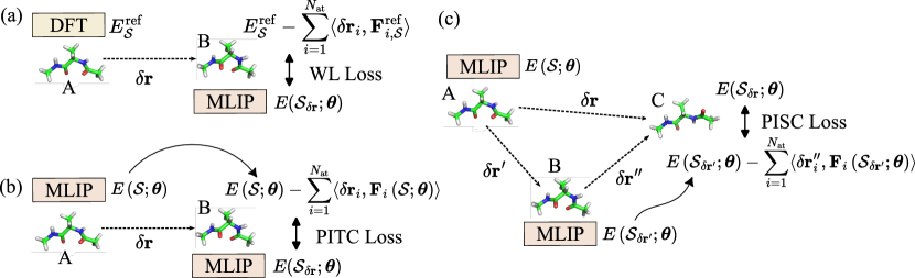
Figure 1: Schematic illustration of physics-informed weakly supervised losses used in this work. (a) Taylor-expansion-based weak label (WL) loss with approximate labels obtained from reference energies and atomic forces [17]. (b) Physics-inspired Taylor-expansion-consistency (PITC) loss with approximate labels obtained from energies and atomic forces predicted by an MLIP. (c) Physics-inspired spatial consistency (PISC) loss with approximate labels obtained from energies and atomic forces predicted by an MLIP. Here, $E(\mathcal{S};\bm{\theta})$ and $\mathbf{F}_{i}(\mathcal{S};\bm{\theta})$ denote the potential energy and atomic forces predicted by an MLIP parametrized by $\bm{\theta}$, $\mathcal{S}$ and $\mathcal{S}_{\delta\mathbf{r}}$ define the original atomic structure and the one perturbed by $\delta\mathbf{r}$.

Contributions. This paper addresses these challenges using a physics-informed weakly supervised learning (PIWSL) approach. Our method is designed to learn an MLIP, which can accurately predict the potential energy and atomistic forces for an atomic system exposed to local perturbations. In particular, our contributions are as follows: (i) We introduce PIWSL based on basic physical principles, such as the concept of conservative forces. We combine it with extrapolating the potential energy via a Taylor expansion and derive two novel physics-informed loss functions, schematically illustrated in Fig. 1 (b) and (c). Particularly, we obtain physics-informed Taylor-expansion-based consistency (PITC) and physics-informed spatial consistency (PISC) losses, which build the basis for the PIWSL approach. (ii) By conducting extensive experiments, we demonstrate that PIWSL facilitates the training of MLIPs without access to large training data sets. (iii) We also observe that PIWSL improves accuracy in predicted total energies and atomic forces, even without access to force labels. This scenario is expected when training MLIPs with reference methods for which calculating atomic forces is infeasible [18, 19, 20]. Thus, our results open new possibilities for training MLIPs using highly accurate energy labels, such as those obtained by extrapolating CCSD(T) energies to the complete basis set (CBS) limit [21, 22]. (iv) Finally, PIWSL mitigates sensitivity issues associated with limited sizes of available data sets by taking into account the potential energy response to local perturbations in atomic structures.

2 Related Work

Machine-Learned Interatomic Potentials. There is a growing interest in using ML-based models for investigating molecular and material systems as they allow performing atomistic simulations with an accuracy on par with first-principles methods but at a fraction of the computational cost. The field of machine-learned interatomic potentials (MLIPs) emerged over two decades ago [23] and has been one of the most active research directions since then [24, 25, 26, 8, 27, 28, 29, 30, 31, 32, 33, 29, 34, 35, 36, 37, 38, 39, 40]. The development of local higher-body-order representations [27, 31, 32, 33] and the emergence of equivariant message-passing neural networks (MPNNs) [29, 34, 35, 36, 37, 38, 39, 40] significantly advanced the field. These methods enable the cost-efficient generation of accurate MLIPs for modeling interactions in many-body atomic systems and account for crucial inductive biases as the invariance of the potential energy under rotation.

Physics-Informed Machine Learning. Physics-informed ML aims to model physical systems using data-driven techniques and incorporates physics principles into ML-based models. For example, MLIPs based on equivariant MPNNs enforce the invariance of the potential energy under rotation and use equivariant features to enrich the building of many-body contributions to it [29, 38, 40, 39, 37]. Furthermore, physics constraints can be integrated via auxiliary loss functions, prompting ML models to learn important physical relationships, as demonstrated for physics-informed neural networks (PINNs) [41, 42], which learn to model solutions of partial differential equations by minimizing residuals during training. Applying physics-informed ML to molecular modeling has gained attraction in both ML and computational chemistry communities [43, 44]. As such, prior work [17] has motivated our current research and is discussed in more detail in subsequent sections.

3 Background and Problem Definition

Machine-Learned Interatomic Potentials. An atomic configuration, denoted as $\mathcal{S}=\{\mathbf{r}_{i},Z_{i}\}_{i=1}^{N_{\mathrm{at}}}$, contains $N_{\mathrm{at}}$ atoms and is defined by atom positions $\mathbf{r}_{i}\in\mathbb{R}^{3}$ and atom types $Z_{i}\in\mathbb{N}$. We consider mapping atomic configurations to scalar energies, i.e., $f_{\bm{\theta}}:\mathcal{S}\mapsto E\in\mathbb{R}$ with $\bm{\theta}$ denoting trainable parameters. We define $E(\mathcal{S};\bm{\theta})$ as the energy predicted by an MLIP for an atomic configuration $\mathcal{S}$. For most MLIPs, atomic forces are computed as the negative gradients of the potential energy with respect to atom positions, i.e., $\mathbf{F}_{i}\left(\mathcal{S};\bm{\theta}\right)=-\nabla_{\mathbf{r}_{i}}E\left(\mathcal{S};\bm{\theta}\right)$. In this way, these MLIPs ensure that the resulting forces are conservative (curl-free) and the total energy is conserved during a dynamic simulation. However, some models are designed to predict atomic forces directly [45, 36, 37, 9]. While this approach avoids expensive gradient computations, it violates the law of energy conservation [46].

Trainable parameters $\bm{\theta}$ are optimized by minimizing loss functions on training data $\mathcal{D}$ comprising a total of $N_{\mathrm{train}}$ atomic configurations $\{\mathcal{S}^{(k)}\}_{k=1}^{N_{\mathrm{train}}}$ as well as their energies $\{E^{\mathrm{ref}}_{\mathcal{S}}\}_{\mathcal{S}\in\mathcal{D}}$ and atomic forces $\{\{\mathbf{F}_{i,\mathcal{S}}^{\mathrm{ref}}\}_{i=1}^{N_{\mathrm{at}}}\}_{\mathcal{S}\in\mathcal{D}}$

$$\mathcal{L}\left(\mathcal{D};\bm{\theta}\right)=\sum_{\mathcal{S}\in\mathcal{D}}L\left(S;\bm{\theta}\right)=\sum_{\mathcal{S}\in\mathcal{D}}\Big{[}C_{\mathrm{e}}\ell\left(E\left(\mathcal{S};\bm{\theta}\right),E^{\mathrm{ref}}_{\mathcal{S}}\right)+C_{\mathrm{f}}\sum_{i=1}^{N_{\mathrm{at}}}\ell\left(\mathbf{F}_{i}(\mathcal{S};\bm{\theta}),\mathbf{F}_{i,\mathcal{S}}^{\mathrm{ref}}\right)\Big{]}.$$ (1)

Here, $\ell$ denotes a point-wise loss function such as the absolute and squared error between the predicted and reference total energies and atomic forces. Typically, reference energies $E^{\mathrm{ref}}_{\mathcal{S}}$ and atomic forces $\mathbf{F}_{i,\mathcal{S}}^{\mathrm{ref}}$ are provided by ab initio or first-principles methods such as CC or DFT, respectively. The relative contributions of energies and forces in Eq. (1) are balanced with the coefficients $C_{\mathrm{e}}$ and $C_{\mathrm{f}}$.

Weakly Supervised Learning. Generating many reference labels with a first-principles approach is challenging due to the high computational cost. Furthermore, the calculation of atomic forces can be infeasible for some high-accuracy ab initio methods, e.g., for CCSD(T)/CBS. In this work, we focus on weakly supervised learning methods to improve the performance of MLIPs in scenarios when only a limited amount of data is available. These involve the generation of approximate but physically motivated total energies for atomic structures generated by small perturbations of their atomic positions, i.e., $\mathcal{S}_{\delta\mathbf{r}}=\{\mathbf{r}_{i}+\delta\mathbf{r}_{i},Z_{i}\}_{i=1}^{N_{\mathrm{at}}}$ with a perturbation vector $\delta\mathbf{r}$ where $\delta\mathbf{r}_{i}$ is the perturbation vector for atom $i$. Approximate labels are computed with MLIPs during their training.

4 Physics-informed Weakly Supervised Learning

For MLIPs, the generation of approximate labels employed in weakly supervised losses is highly non-trivial. Small perturbationss in atomic structures can lead to significant changes in energies and atomic forces. Thus, standard approaches that are effective for many ML tasks [47] are typically not applicable to MLIPs. To address this problem, we propose a physics-informed weakly supervised learning approach that involves (i) a Taylor expansion of the potential energy for computing the response to atomic perturbations and (ii) spatial consistency to estimate the displaced potential energy based on the concept of conservative forces. We finally introduce the PIWSL loss term, combining both classes of weakly supervised loss functions with the supervised loss.

4.1 Physics-Informed Taylor-Expansion-Based Consistency Loss

This section introduces the physics-informed Taylor-expansion-based consistency (PITC) loss. Particularly, we relate the energy predicted directly for a displaced atomic configuration with the energy obtained by the Taylor expansion from the original configuration; see Fig. 1 (b). We estimate the energy for an atomic structure $\mathcal{S}$ drawn from the training data set with atomic positions displaced by a vector $\delta\mathbf{r}$: $\mathcal{S}_{\delta\mathbf{r}}=\{\mathbf{r}_{i}+\delta\mathbf{r}_{i},Z_{i}\}_{i=1}^{N_{\mathrm{at}}}$. For this atomic configuration, we expand the energy predicted by an MLIP in its first-order Taylor series around the atomic perturbation vector $\delta\mathbf{r}_{i}$ and obtain

$$\begin{split}E\left(\mathcal{S}_{\delta\mathbf{r}};\bm{\theta}\right)&\approx E\left(\mathcal{S};\bm{\theta}\right)-\sum_{i=1}^{N_{\mathrm{at}}}\langle\delta\mathbf{r}_{i},\mathbf{F}_{i}\left(\mathcal{S};\bm{\theta}\right)\rangle+\mathcal{O}\left(\|\delta\mathbf{r}\|^{2}\right),\end{split}$$ (2)

where $\langle\cdot\rangle$ denotes the inner product. Here, we used that atomic forces are defined as the negative gradients of the potential energy. For small magnitudes of $\delta\mathbf{r}_{i}$, the second order term $\mathcal{O}\left(\|\delta\mathbf{r}\|^{2}\right)$ in Eq. (2) can be neglected. Using approximate labels $E\left(\mathcal{S}_{\delta\mathbf{r}};\bm{\theta}\right)$, we define the PITC loss as

$$\begin{split}L_{\mathrm{PITC}}\left(\mathcal{S};\bm{\theta}\right)&=\ell\Big{(}E\left(\mathcal{S}_{\delta\mathbf{r}};\bm{\theta}\right),E\left(\mathcal{S};\bm{\theta}\right)-\sum_{i=1}^{N_{\mathrm{at}}}\langle\delta\mathbf{r}_{i},\mathbf{F}_{i}\left(\mathcal{S};\bm{\theta}\right)\rangle\Big{)},\end{split}$$ (3)

where $\ell$ denotes a point-wise loss for regression problems and $\delta\bm{r}$ is randomly-sampled or determined adversarially; see Section 4.4 for more details. Hence, whenever we encounter a structure $\mathcal{S}$ in a batch during training, a new $\delta\bm{r}$ is computed for each $\mathcal{S}$.

4.2 Physics-Informed Spatial-Consistency Loss

This section introduces a physics-informed approach for generating weak labels based on the concept of conservative forces. Thus, we leverage that the energy difference between two points on the potential energy surface is independent of the path taken between them. We consider two paths from a reference point to the same target point, composed of three perturbation vectors in total. We estimate the potential energy at the target point via Eq. (2). An example of two paths is demonstrated in Fig. 1 (c). The figure relates the energy obtained when displacing atomic positions of the original configuration $\mathcal{S}$ (denoted by A in the figure) by $\delta\mathbf{r}$ (from configuration A to C) with the energy obtained through consecutive perturbations $\delta\mathbf{r}^{\prime}$ (from configuration A to B) and $\delta\mathbf{r}^{\prime\prime}$ (from configuration B to C).

For the first path, we directly predict the energy with an MLIP, i.e., $E\left(\mathcal{S}_{\delta\mathbf{r}};\bm{\theta}\right)$, which is related to the approximated energy at $\mathbf{r}+\delta\mathbf{r}$ using Eq. (3) through PITC loss. For the second path, we directly compute the energy $E\left(\mathcal{S}_{\delta\mathbf{r}^{\prime}};\bm{\theta}\right)$ for atomic positions displaced by $\delta\mathbf{r}^{\prime}$ and use it to approximate $E\left(\mathcal{S}_{\delta\mathbf{r}};\bm{\theta}\right)$ after applying the second perturbation vector $\delta\mathbf{r}^{\prime\prime}\equiv\delta\mathbf{r}-\delta\mathbf{r}^{\prime}$. The physics-informed spatial consistency (PISC) loss can be defined as

$$\begin{split}L_{\mathrm{PISC}}\left(\mathcal{S};\bm{\theta}\right)&=\ell\Big{(}E\left(\mathcal{S}_{\delta\mathbf{r}};\bm{\theta}\right),E\left(\mathcal{S}_{\delta\mathbf{r}^{\prime}};\bm{\theta}\right)-\sum_{i=1}^{N_{\mathrm{at}}}\langle\delta\mathbf{r}_{i}^{\prime\prime},\mathbf{F}_{i}\left(\mathcal{S}_{\delta\mathbf{r}^{\prime}};\bm{\theta}\right)\rangle\Big{)},\end{split}$$ (4)

where $\delta\mathbf{r}$ is randomly-sampled or determined adversarially; see Section 4.4. After joint training of PITC and PISC losses, the three different estimations at $\mathcal{S}_{\delta\mathbf{r}}$ become spatially consistent. Note that our conservative forces-based approach is not limited to relations between two perturbation paths or three perturbation vectors. We discuss several other possible configurations in Section D.3.

4.3 Combined Physics-Informed Weakly Supervised Loss

Together with the usual MLIP loss function given in Eq. (1), the overall objective, which we refer to as the PIWSL loss, can be written as

$$\operatorname*{arg\,min}_{\bm{\theta}}\tilde{\mathcal{L}}\left(\mathcal{D};\bm{\theta}\right)=\operatorname*{arg\,min}_{\bm{\theta}}\sum_{\mathcal{S}\in\mathcal{D}}\left(L\left(\mathcal{S};\bm{\theta}\right)+C_{\mathrm{PITC}}L_{\mathrm{PITC}}\left(\mathcal{S};\bm{\theta}\right)+C_{\mathrm{PISC}}L_{\mathrm{PISC}}\left(\mathcal{S};\bm{\theta}\right)\right),$$ (5)

where $C_{\rm PITC}$ and $C_{\rm PISC}$ are the weights of the weakly supervised PITC and PISC losses.

4.4 Determining Perturbation Directions and Magnitudes

The effectiveness of the proposed approach depends on appropriate choices of the perturbation vectors $\delta\mathbf{r}$. Therefore, we introduce and justify various generation strategies for the perturbations $\delta\mathbf{r}$ used in Eq. (3) and Eq. (4). We can express any vector $\delta\mathbf{r}$ as $\delta\mathbf{r}\equiv\epsilon\mathbf{g}/\|\mathbf{g}\|_{2}$, where $\epsilon$ is the magnitude of $\delta\mathbf{r}$ and $\mathbf{g}/\|\mathbf{g}\|_{2}$ represents the direction of $\delta\mathbf{r}$. Physical constraints are considered when determining $\epsilon$. Specifically, the maximum length of the perturbation can be obtained from the validity of the Taylor expansion in Eq. (2), which, as discussed in Section 5.3, is typically given as at most 30% of the original bond length whose shortest example is the bond between carbon and hydrogen, about 1.09 Å; see also Fig. 2 (c) and (d). The specific values of $\epsilon$ chosen for our experiments are provided in Section B.1.

To determine $\mathbf{g}/\|\mathbf{g}\|_{2}$ we explore two strategies. First, we compute it as the unit vector of a perturbation vector sampled from the uniform distribution on the interval $(-1,1)$ for each direction

$$\delta\mathbf{r}_{\rm rnd}\equiv\epsilon\mathbf{g}/\|\mathbf{g}\|_{2}.$$ (6)

Second, we compute an adversarial direction, as proposed elsewhere [48, 49], which involves defining it as the direction (the gradients) in which the loss error increases the most at the current atom coordinates $\mathbf{r}$ and for the current predicted energy. Assuming the norm of adversarial perturbation as $L_{2}$, the adversarial direction can be approximated by [49]

$$\delta\mathbf{r}_{\rm adv}\equiv\epsilon\mathbf{g}/\|\mathbf{g}\|_{2},\ {\rm where}\ \mathbf{g}=\nabla_{\mathbf{r}}L_{\rm dist}(\mathbf{y}^{\rm pred},\mathbf{y}^{\rm ref}),$$ (7)

where $L_{\rm dist}$ is a distance measure function to be maximized by adding $\delta\mathbf{r}_{\rm adv}$, with $\mathbf{y}^{\rm pred}$ and $\mathbf{y}^{\rm ref}$ being the ML model prediction and the reference values. Due to their computational efficiency, we mainly use Eq. (6) in our experiments. A quantitative comparison between the random and adversarial directions is provided in Section 5.5.

5 Experiments

We evaluate our method with an extensive set of experiments with the following objectives: (1) a comparison of the PIWSL method with existing baselines, (2) a detailed analysis of the impact of the PIWSL method using the aspirin molecule, (3) an exploration of the ability of PIWSL to improve energy and force predictions when force labels are inaccessible, (4) a comparison to prior work that used a weakly supervised approach, (5) an ablation study, and (6) a comparison between random and adversarial generation of the perturbation vector. In general, we focus on the data-scarce setting where the number of training samples is between $100$ and $1000$ since the computational cost of ab initio and first-principles approaches to generate large data sets can be prohibitive.

Table 1: Energy (E) and force (F) root-mean-square errors (RMSEs) for the ANI-1x data set. The results are obtained by averaging over three independent runs. Energy RMSE is given in kcal/mol, while force RMSE is in kcal/mol/Å.

		$N_{\mathrm{train}}=100$			$N_{\mathrm{train}}=1000$
		Baseline	Noisy Nodes	PIWSL	Baseline	Noisy Nodes	PIWSL
SchNet	E	65.09 $\pm$ 2.42	57.39 $\pm$ 0.05	60.30 $\pm$ 1.77	31.49 $\pm$ 0.01	31.10 $\pm$ 0.00	31.50 $\pm$ 0.00
	F	29.06 $\pm$ 0.19	25.62 $\pm$ 0.01	28.20 $\pm$ 0.60	18.94 $\pm$ 0.01	18.10 $\pm$ 0.00	18.93 $\pm$ 0.00
PaiNN	E	168.01 $\pm$ 1.22	464.55 $\pm$ 6.91	109.89 $\pm$ 11.46	56.62 $\pm$ 2.80	305.76 $\pm$ 33.93	24.53 $\pm$ 0.48
	F	21.33 $\pm$ 0.10	20.82 $\pm$ 0.03	18.76 $\pm$ 0.30	12.96 $\pm$ 0.06	14.25 $\pm$ 0.18	11.43 $\pm$ 0.05
SpinConv	E	162.14 $\pm$ 7.55	147.73 $\pm$ 2.23	130.97 $\pm$ 8.58	43.59 $\pm$ 1.71	299.33 $\pm$ 419.10	39.44 $\pm$ 1.31
	F	21.22 $\pm$ 0.43	21.08 $\pm$ 0.43	21.61 $\pm$ 0.44	14.51 $\pm$ 1.07	15.83 $\pm$ 0.75	13.59 $\pm$ 0.20
eSCN	E	214.52 $\pm$ 7.55	521.92 $\pm$ 12.05	183.70 $\pm$ 9.79	59.59 $\pm$ 8.92	241.34 $\pm$ 20.16	21.03 $\pm$ 0.56
	F	20.07 $\pm$ 0.27	23.68 $\pm$ 0.11	19.69 $\pm$ 0.05	12.50 $\pm$ 0.78	14.42 $\pm$ 0.84	11.83 $\pm$ 0.12
Equiformer	E	398.71 $\pm$ 13.69	632.38 $\pm$ 0.11	154.98 $\pm$ 8.83	54.52 $\pm$ 4.52	854.33 $\pm$ 317.7	20.89 $\pm$ 0.50
	F	20.71 $\pm$ 0.05	21.82 $\pm$ 0.01	20.55 $\pm$ 0.05	10.10 $\pm$ 0.00	24.79 $\pm$ 2.05	9.68 $\pm$ 0.03

5.1 Models and Data Sets

We trained the following representative models that are provided in the Open Catalyst code base [9]: SchNet  [28], PaiNN [34], SpinConv [35], eSCN [36], and Equiformer v2 [37], covering MLIPs with a smaller (SchNet, SpinConv) and larger number of parameters (eSCN, Equiformer v2). Moreover, we also considered a parameter-efficient PaiNN model. Unless otherwise mentioned and except for SchNet, forces are directly predicted and not computed through the negative gradient of the energy. The results where forces are computed as negative energy gradients are analyzed in Section 5.4 and Section D.9. To evaluate the effect and dependency of the physics-informed weakly supervised approach in detail, we performed the training on various data sets: ANI-1x as a heterogeneous molecular data set [19], TiO₂ as a data set for inorganic materials [26], the revised MD17 (rMD17) data set containing small molecules with sampled configurational spaces for each [46, 50, 51], and LMNTO as another material data set [17]; the results for rMD17 and LMNTO are provided in Section D.1. The detailed description of each data set is provided in Section B.3.

5.2 Benchmark Results

We compare models trained using the PIWSL loss (see Eq. (5)) with baseline models trained using the standard supervised loss only (see Eq. (1)). We also compare our approach to a recently proposed data augmentation method that incorporates the task of denoising random perturbations of the atomic coordinates into the learning objective (NoisyNode) [43]. More details on the setup are provided in Section B.1.

Heterogeneous Molecular Data Set (ANI-1x). The results provided in Table 1 show that our approach improves the baseline models’ performance in almost all cases. In particular, the error reduction for the predicted energies is often between $10$ % and more than $50$ %. Interestingly, we observe an improved accuracy for potential energies and atomic forces because we include force prediction in PITC and PISC losses, different from the previous work [17]. In most cases, except for SchNet, the data augmentation method (NoisyNode) degrades the accuracy of the MLIPs because it does not incorporate the proper response of the energy and atomic forces to the perturbation of atomic positions.

Table 2: Energy (F) and force (F) root-mean-square errors (RMSEs) for the TiO₂ data set. The results are obtained by averaging over three independent runs. Energy RMSE is given in kcal/mol, while force RMSE is in kcal/mol/Å.

		$N_{\mathrm{train}}=100$			$N_{\mathrm{train}}=1000$
		Baseline	Noisy Nodes	PIWSL	Baseline	Noisy Nodes	PIWSL
SchNeta	E	17.21 $\pm$ 0.00	19.68 $\pm$ 0.00	17.08 $\pm$ 0.00	9.56 $\pm$ 0.00	9.60 $\pm$ 0.00	9.51 $\pm$ 0.00
	F	2.84 $\pm$ 0.00	2.70 $\pm$ 0.00	2.83 $\pm$ 0.00	2.14 $\pm$ 0.00	2.15 $\pm$ 0.00	2.13 $\pm$ 0.00
PaiNNb	E	14.41 $\pm$ 0.16	n/ab	13.95 $\pm$ 0.09	4.49 $\pm$ 0.15	n/ab	3.63 $\pm$ 0.20
	F	1.59 $\pm$ 0.01	n/ab	1.56 $\pm$ 0.01	0.41 $\pm$ 0.02	n/ab	0.34 $\pm$ 0.01
SpinConv	E	20.00 $\pm$ 0.42	18.76 $\pm$ 0.74	16.98 $\pm$ 0.99	4.17 $\pm$ 0.76	4.09 $\pm$ 0.65	2.50 $\pm$ 0.40
	F	1.58 $\pm$ 0.03	1.53 $\pm$ 0.03	1.59 $\pm$ 0.03	0.65 $\pm$ 0.02	0.71 $\pm$ 0.16	0.58 $\pm$ 0.05
eSCN	E	16.41 $\pm$ 1.10	20.92 $\pm$ 0.00	12.63 $\pm$ 0.78	3.31 $\pm$ 1.18	20.90 $\pm$ 0.01	1.40 $\pm$ 0.10
	F	1.57 $\pm$ 0.04	1.66 $\pm$ 0.00	1.44 $\pm$ 0.03	0.46 $\pm$ 0.23	1.66 $\pm$ 0.00	0.21 $\pm$ 0.00
Equiformer	E	18.21 $\pm$ 0.02	19.06 $\pm$ 0.02	13.93 $\pm$ 0.09	3.67 $\pm$ 0.03	18.75 $\pm$ 0.05	1.82 $\pm$ 0.34
	F	1.56 $\pm$ 0.01	1.64 $\pm$ 0.00	1.51 $\pm$ 0.19	0.17 $\pm$ 0.01	1.58 $\pm$ 0.00	0.17 $\pm$ 0.01

^a We used a larger batch size of $32$ for SchNet since we obtained extremely high errors for the batch size of $4$. A more detailed discussion of the experimental results for SchNet is provided in Section D.1.
^b Because of a numerical instability of PaiNN when perturbing atomic coordinates, the cutoff radius is reduced from 12 Å to 5 Å in this experiment. Predicted values become n/a when perturbations are added to atomic configurations.

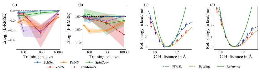
Figure 2: (a, b) Relative performance gains for MLIPs trained with PIWSL compared to those trained without it and (c, d) Potential energy profiles for a C–H bond of the aspirin molecule. Relative performance gains are evaluated for (a) energy (E-) and (b) force (F-) RMSEs. These results are presented for the ANI-1x data set. Potential energy profiles for a C–H bond of the aspirin molecule are presented for models trained using (c) 100 and (d) 200 configurations. The red and blue arrows indicate the direction from the original structure ($E(\mathcal{S};\bm{\theta})$) to the perturbed one ($E(\mathcal{S}_{\delta\mathbf{r}};\bm{\theta})$), as defined by Eq. (2), for the baseline and PIWSL model predictions, respectively.

Table 3: Results for models trained on the ANI-1x data set without reference forces. All models are trained using 1000 training samples. FB refers to the setting where the force branch estimates the force, and GB denotes the setting where the force is estimated by the gradient of the potential energy with respect to the atomic coordinates.

Model	Case		Baseline	PIWSL
PaiNN	FB	E	42.36 $\pm$ 0.30	25.42 $\pm$ 0.72
		F	24.25 $\pm$ 0.00	20.54 $\pm$ 0.08
	GF	E	41.83 $\pm$ 1.81	29.71 $\pm$ 0.55
		F	83.36 $\pm$ 2.85	24.02 $\pm$ 0.95
Equiformer	FB	E	43.14 $\pm$ 0.86	29.48 $\pm$ 0.51
		F	24.25 $\pm$ 0.00	21.99 $\pm$ 0.49
	GF	E	42.55 $\pm$ 0.99	32.66 $\pm$ 1.11
		F	35.70 $\pm$ 0.78	21.83 $\pm$ 0.27

Table 4: Results for models trained on the ANI-1x data set with ablated weakly supervised losses. All models are trained using 1000 training samples. All results are obtained by averaging over three independent runs. Energy RMSE is given in kcal/mol, while force RMSE is given in kcal/mol/Å.

Model	PITC	PISC	E	F
PaiNN	✗	✗	56.62 $\pm$ 2.80	12.96 $\pm$ 0.06
	✓	✗	24.60 $\pm$ 0.18	11.51 $\pm$ 0.03
	✗	✓	58.30 $\pm$ 2.10	13.18 $\pm$ 0.29
	✓	✓	24.53 $\pm$ 0.48	11.43 $\pm$ 0.05
Equiformer	✗	✗	54.52 $\pm$ 4.52	10.10 $\pm$ 0.00
	✓	✗	32.64 $\pm$ 26.48	9.64 $\pm$ 0.03
	✗	✓	48.96 $\pm$ 4.96	10.30 $\pm$ 0.06
	✓	✓	20.89 $\pm$ 0.50	9.68 $\pm$ 0.03

Training Data Set Size Dependence (ANI-1x). We train MLIPs with training set sizes of $[50,10^{2},10^{3},10^{4}]$. The results are plotted in Fig. 2 (a) and (b). Although the observed error reduction depends strongly on the type of MLIP used, the benefit of the weakly supervised losses often decreases slightly with the number of training samples. This result can be expected as the area covered by the weakly supervised losses is also gradually covered by the reference data as the number of training samples increases. Moreover, the gain in accuracy of energy predictions is more significant than that for forces trained only indirectly through the consistency constraint in PITC; see Eq. (3). Finally, it is shown that the improvement is more significant for highly parameterized MLIPs, which benefit the most from increasing the training data size through PIWSL.

Inorganic Bulk Materials (TiO₂). Titanium dioxide (TiO₂) is a highly relevant metal oxide for industrial applications, featuring several high-pressure phases. Thus, ML models should be able to predict total energies and atomic forces for various high-pressure phases of TiO₂, considering periodic boundaries (relevant when aggregating over the local atomic neighborhood). The results for trained models are provided in Table 2. Similar to the ANI-1x data set, our approach improves the accuracy of predicted energies and atomic forces. Interestingly, although the error in the potential energy for 1000 training configurations reaches small RMSE values, from 2 to 4 kcal/mol in predicted energy, the PIWSL still provides a further error reduction. This observation indicates strong evidence of the effectiveness of PIWSL applied to bulk materials.

5.3 Qualitative Impact of PIWSL

We evaluate the prediction variance and robustness of an MLIP model trained with PIWSL using the aspirin molecule, focusing on the potential energy’s dependence on the C–H bond length. In this work, robustness refers to the prediction robustness of an MLIP to perturbations in atomic coordinates. In literature, the robustness of MLIPs often means their stability during MD simulations, which is outside the scope of this paper. We train PaiNN on the rMD17 aspirin data set using $100$ and $200$ configurations with and without the PIWSL loss. The detailed training setup and errors of the used MLIPs are summarized in Section D.4. We examine the potential energy varying the length of a C–H bond from $0.9$ Å to $1.4$ Å. The equilibrium C–H bond length is about $1.09$ Å. The results in Fig. 2 (c) and (d) show that the PIWSL method improves the predicted potential energy profile, demonstrating increased robustness under perturbations of atom coordinates. This improvement in the potential curve prediction is achieved without introducing unphysical noise, which can occur when using inappropriate weak labels for the perturbed atomic coordinates.

Although the estimated potential energies do not always match the reference values, the direction between the original and perturbed configurations, indicated by arrows in Fig. 2, consistently follows the gradient of the reference potential energy, corresponding to the negative force. In Fig. 2, we use a perturbation length of $||\delta\mathbf{r}||=0.01$ Å. This consistency with the energy gradient underscores the PIWSL method’s effectiveness, ensuring the alignment between predicted total energies and force and improving the corresponding RMSE values. As discussed in Section 4.2, PIWSL also addresses the limitation of MLIPs that employ separate force branches and do not guarantee the prediction of conservative forces. The proposed method reduces the curl of predicted forces, as detailed in Section D.11, although complete elimination of the curl remains a challenge. In summary, PIWSL minimizes individual energy and force errors, improving the overall accuracy of MLIPs.

5.4 Training MLIPs without Reference Forces

In the following, we explore scenarios where only potential energy labels are available. This situation commonly arises when calculating energy labels with chemically accurate approaches, such as CCSD(T)/CBS [21, 22], for which force calculation is infeasible. To consider practical applications, we examine two cases: (1) predicting force by a force branch (FB) and (2) predicting force as a gradient of the potential energy (GF). The former enables fast force prediction and is popular in the machine learning community, while the latter requires additional gradient calculation but yields curl-free force predictions. It is popular in computational chemistry as it ensures the conservation of the total energy during MD simulations. The results are provided in Table 3; training without reference forces is achieved by setting the relative force contribution to zero in Eq. (1). The PIWSL method consistently performs better than the baseline for the FB and GF cases. However, a more significant improvement in the force prediction performance is observed in the GF case. We attribute this phenomenon to the inherent nature of PIWSL, which requires consistency between the potential energy and atomic forces, as discussed in Section 5.3. This result aligns with our expectations, confirming the capability of our PIWSL method to enable ML models to reduce the error in the predicted forces. Overall, PIWSL opens a new possibility for training MLIP models using highly accurate reference methods, such as CCSD(T)/CBS.

5.5 Further Analyses of PIWSL

The following provides further analyses of our approach. We provide the results for Equiformer v2 and PaiNN since these models employ equivariant features and demonstrate a high accuracy on the ANI-1x data set when trained using 1000 configurations.

Comparing PITC with the Taylor-Expansion-Based Weak Label Loss. We compare our proposed method with the Taylor-expansion-based weak label (WL) approach [17]. For the WL method, we utilize Eq. (A3) as the loss function. For simplicity, we only consider the PITC loss in Eq. (3). For a fair comparison, we consider the following two cases. First, we train with reference forces and energies (w. RF). Second, we train the methods without reference forces and use only the reference energies. For the training with reference forces, we set the numeric coefficient of the PITC loss to $1.0$; for the training without reference forces, the coefficient is set to $0.1$. The results are provided in Table 5.

Our PITC loss demonstrates the best accuracy in all cases, with and without the reference forces. Interestingly, PaiNN failed to learn the potential energy with the WL loss and reference forces. We hypothesize this to be due to the imbalance of the training between the energies and forces. Specifically, the WL loss trains only the potential energy, resulting in an inconsistency between the energy and force branches, which share the same readout layer that experiences more frequent updates using the potential energy. This hypothesis is supported by the results for the training without reference forces, where the error in energy is reduced compared to the baseline. A further validation in a similar experiment in the case of GF is provided in Section D.9. However, the proposed PITC loss still performs better here. In summary, the PITC loss enables MLIPs to learn energies and forces consistent with each other and does it better than the previously proposed WL method.

Table 5: Comparison of PITC and the Taylor-expansion-based weak label loss. WL denotes the Taylor-expansion-based method using reference energies and atomic forces; see Eq. (A3). The listed values are the RMSE values for energies in kcal/mol and atomic forces in kcal/mol/Å. All models are trained on the ANI-1x data set using 1000 configurations, with (w.) and without (w/o.) reference atomic forces (RF).

Model	Case		Baseline	PITC	WL
PaiNN	(w. RF)	E	56.62 $\pm$ 2.80	30.94$\pm$ 0.56	81.86$\pm$ 9.39
		F	12.96$\pm$ 0.06	12.04$\pm$ 0.04	14.54$\pm$ 0.12
	(w/o. RF)	E	42.36$\pm$ 0.30	25.42$\pm$ 0.72	35.79$\pm$ 0.70
		F	24.25$\pm$ 0.00	20.54$\pm$ 0.08	24.25$\pm$ 0.01
Equiformer	(w. RF)	E	54.52$\pm$ 4.52	23.16$\pm$ 0.19	31.02$\pm$ 3.99
		F	10.10$\pm$ 0.00	10.03$\pm$ 0.05	13.43$\pm$ 0.92
	(w/o. RF)	E	43.14$\pm$ 0.86	29.48$\pm$ 0.51	30.08$\pm$ 1.97
		F	24.25$\pm$ 0.00	21.99$\pm$ 0.49	24.25$\pm$ 0.00

Ablating the Impact of PITC and PISC Losses. We conduct an ablation experiment to analyze the impact of PITC and PISC losses. Results in Table 5.2 indicate that the PITC loss predominantly improves the accuracy of resulting models, especially for PaiNN. Using just the PISC loss does not consistently improve accuracy but stabilizes training when combined with PITC. This combined approach notably benefits Equiformer v2. For Equiformer v2, we repeated the experiment five times to reduce the effect from an outlier for the PITC loss.

Adversarial Directions for Perturbing Atomic Positions. The following discusses the dependence of the PIWSL’s performance on selecting the vector $\delta\mathbf{r}$ in Eq. (5) employed to perturb atomic positions. The detailed implementation and setups are provided in Section B.1. Table 6 compares the results obtained for a randomly-sampled vector $\delta\mathbf{r}$ and for the one determined adversarially. The results demonstrate that both approaches improve the performance compared to the baseline without weak supervision, though the results might depend on the employed model.

Table 6: Dependence of the PIWSL’s performance on the atomic position perturbation vector. The listed numerical values are the root mean square errors (RMSEs) for the energy in kcal/mol and force in kcal/mol/Å. All results are provided for the ANI-1x data set and models trained using 1000 configurations.

		Baseline	Random (Eq. (6))	Adversarial (Eq. (7))
PaiNN	E	56.62 $\pm$ 2.80	24.53 $\pm$ 0.48	33.67 $\pm$ 1.12
	F	12.96 $\pm$ 0.18	11.43 $\pm$ 0.05	12.74$\pm$ 0.14
Equiformer	E	54.52 $\pm$ 4.52	23.16 $\pm$ 0.50	20.54$\pm$ 0.21
	F	10.10 $\pm$ 0.00	10.03 $\pm$ 0.03	9.93$\pm$ 0.04

6 Discussion and Limitations

This work introduces the PIWSL method, encompassing two distinct physics-informed weakly supervised loss functions, for learning MLIPs. These losses provide the physics-informed weak labels based on the Taylor expansion (PITC loss) and the spatial-consistency (PISC loss) of the potential energy. These physics-informed weak labels enable any MLIP to improve its accuracy, particularly in scenarios characterized by small training data set sizes. Such scenarios are common when investigating a new molecular or material system. Our extensive experiments demonstrate notable efficacy and efficiency of our method from various aspects: (i) dependence on the training data set size, (ii) the potential energy prediction variance and robustness in terms of a perturbation on a C–H bond length, and (iii) selection of the perturbation vector. In particular, it is shown that our PIWSL method enables ML models to improve the force prediction even without force labels, thereby opening a new possibility for training MLIPs using highly accurate reference methods, such as CCSD(T)/CBS.

Limitations. The proposed PIWSL method is tailored to ML models that predict atomic forces and total energies of atomic systems. It cannot be applied to other ML problems unrelated to computational chemistry or materials science applications. Although this work uses the first-order Taylor expansion to obtain weak labels in Eq. (2), employing a more sophisticated higher-order ordinary differential equation solver is a viable alternative.

Code availability

The source code will be made publicly available upon publication.

Appendix A Related Work

Addressing Data Sparsity in MLIPs. Generating training data sets suitable for learning reliable MLIPs is challenging, especially when considering unexplored molecular and material systems. Numerous computationally expensive calculations with either ab initio or first-principles approaches are required for the latter. To mitigate this challenge, active learning (AL) methods, which utilize prediction uncertainty, can be applied [14, 52, 15, 53, 54, 16]. Furthermore, equivariant MLIPs often reduce required training data set sizes through improved data efficiency [38, 40].

Appendix B Experimental Setup, Baselines, and Data Sets

B.1 Experimental Setup

Code for Experiments. The code used to run our experiments builds upon the recent work [55] and extends it to integrate the latest Open Catalyst Project code [9]. We adopt hyper-parameters from the Open Catalyst (OC) project, tuned to the corresponding OC data set. Note that we do not use this data set in the presented work, whose main focus is training general-purpose MLIPs that can be used to run molecular dynamics (MD) simulations and geometry optimization. However, the OC data set has been designed to investigate the latter, making it less suitable for the current study. Our modifications include adjusting the learning rate scheduler, details of which can be found in our repository. For potential energy and force prediction, we utilize mean-absolute error (MAE) and $L_{2}$-norm (L2MAE) losses with coefficients of 1 and 100, respectively. More details on the model hyperparameters are provided in our repository. For the PITC and PISC loss functions, we use the mean square error (MSE) loss based on an experiment in Section D.5.

Table A1: Employed mini-batch sizes. We provide mini-batch sized for all data sets and models employed in this work.

	ANI-1x	TiO2a	rMD17	LMNTO
Mini-batch size	6	4	16	4

^a As explained in Table 2, the mini-batch size of the SchNet model was changed to 32 due to high RMSE values observed with a mini-batch size of four as the training data set size increased. A more detailed discussion of the results for SchNet is provided in Section D.1.

Table A2: Total number of training iterations. We provide the total number of training iterations for all data sets and training set sizes employed in this work. The number in the parentheses demonstrates the corresponding total number of training epochs.

$N_{\mathrm{train}}$	ANI-1x	TiO2	rMD17	LMNTO
50	7500 (900)	–	–	–
100	10,000 (600)	10,000 (400)	7500 (1200)	10,000 (400)
1000	40,000 (240)	10,000 (100)	10,000 (160)	10,000 (100)
10,000	100,000 (60)	–	–	–

Training Details. For training MLIPs, we followed the setup in the Open Catalyst Project. We kept the mini-batch size consistent across all models, as shown in Table A1. We have chosen the mini-batch size based on the maximum memory needed by the most demanding models, such as eSCN and Equiformer v2. All experiments are performed on a single NVIDIA A100 GPU with 81.92 GB memory. To avoid overfitting, we stopped training when the validation loss stopped improving—the specific number of training iterations is provided in Table A2.

We used perturbation vectors $\delta\mathbf{r}$ drawn from a uniform random distribution; see also Section 4.4. Particularly, we defined $\delta\mathbf{r}\equiv\epsilon\mathbf{g}$, with each component of $\mathbf{g}$ drawn from a uniform random distribution in the interval $(-1,1)$. The magnitude $\epsilon$ is also drawn from a uniform random distribution and $\epsilon<\epsilon_{\mathrm{max}}$. This definition of $\delta\mathbf{r}$ differs from the one in Eq. (6), improving the computational efficiency of PIWSL by avoiding the calculation of square root and division.

The remaining hyper-parameters are the coefficients for the PITC and PISC losses ($C_{\rm PITC},C_{\rm PISC}$) and the maximum magnitude $\epsilon_{\mathrm{max}}$ of the perturbation vector $\delta\mathbf{r}$; see Table A3. These hyper-parameters are tuned using Optuna [56] for PaiNN and Equiformer v2. We used 1000 configurations drawn randomly from the original ANI-1x data set for training. Due to multiple local minima, Optuna identified several optimal hyper-parameter sets in each run. We selected the following representative combinations ($C_{\rm PITC},C_{\rm PISC},\epsilon_{\mathrm{max}})$ = Case A: (1.2, 0.8, 0.025), Case B: (1.0, 0, 0.01), Case C: (0.1, 0.01, 0.01), Case D: (1.2, 0.01, 0.025), Case E: (1.2, 0.01, 0.01), Case F: (1.2, 0.01, 0.015), Case G: (0.01, 0.001, 0.025), and Case H: (0.1, 0.01, 0.025).

Table A3: Hyper-parameters for the PIWSL loss. We selected the following hyper-parameter combinations using Optuna [56]: ($C_{\rm PITC},C_{\rm PISC},\epsilon_{\mathrm{max}})$= Case A: (1.2, 0.8, 0.025), Case B: (1.0, 0, 0.01), Case C: (0.1, 0.01, 0.01), Case D: (1.2, 0.01, 0.025), Case E: (1.2, 0.01, 0.01), Case F: (1.2, 0.01, 0.015), Case G: (0.01, 0.001, 0.025), and Case H: (0.1, 0.01, 0.025).

Dataset	Size	Equiformer v2	eSCN	PaiNN	SpinConv	SchNet
ANI-1x	50	A	C	B	A	A
	100	A	C	A	D	A
	1000	D	D	D	B	B
	10,000	G	C	B	C	C
TiO2	100	A	A	A	A	H
	1000	G	A	C	A	C
rMD17	100	E	B	F	D	A
(Aspirin)	1000	B	B	B	B	B
rMD17	100	B	B	B	B	B
(Benzene)	1000	G	B	B	B	B
rMD17	100	G	B	B	B	B
(Naphthalene)	1000	G	B	B	B	B
LMNTO	100	B	B	B	A	B
	1000	B	A	B	B	B

Splitting Data Sets. We split the original data sets into training, validation, and test sets for our experiments. We shuffled the original data sets using a random seed and selected the training data sets of predefined sizes. For validation, we selected the same number of configurations as in the training data set if it exceeded 100 configurations; otherwise, we used 100 configurations to ensure sufficient validation size. For the rMD17 data set, following [55], we used 9000 configurations as a validation data set and another 10,000 for testing. We used the same test data set across different sizes of the training data sets for a fair performance comparison. We used 10,000 test configurations for ANI-1x and 1000 for TiO₂ and LMNTO.

Training with Adversarial Directions. In our experiments, which defined perturbation vectors adversarially (see Section 5.5), we determined adversarial directions using Eq. (7). More concretely, we only considered the potential energy, i.e., $\mathbf{y}_{\rm pred}$ and $\mathbf{y}_{\rm label}$, to avoid Hessian calculations. In addition, we considered the loss function for the potential energy as $L_{\rm dist}$ in Eq. (7). The expression of $\mathbf{g}=\nabla_{\mathbf{r}}L_{\rm dist}$ is then

$$\mathbf{g}_{\mathcal{S}}=\nabla_{\mathbf{r}_{i}}\sqrt{(E\left(\mathcal{S};\bm{\theta}\right)-E^{\rm ref}_{\mathcal{S}})^{2}}=-\frac{1}{2L_{\rm dist}}(\mathbf{F}_{i}\left(\mathcal{S};\bm{\theta}\right)-\mathbf{F}^{\rm ref}_{i,\mathcal{S}})(E\left(\mathcal{S};\bm{\theta}\right)-E^{\rm ref}_{\mathcal{S}}).$$ (A1)

Note that we used the relation: $\nabla_{\mathbf{r}_{i}}E^{\rm ref}_{\mathcal{S}}=-\mathbf{F}^{\rm ref}_{i,\mathcal{S}}$, to obtain the final expression. Though $E^{\rm ref}$ can also be interpreted as a constant regarding atom positions. We have chosen this expression to avoid the case where the adversarial direction $\mathbf{g}$ points to $\mathbf{F}^{\rm ref}_{i,\mathcal{S}}$ other than the very beginning of the training. Our experiments indicate that the employed expression is slightly better than its alternative. In our experiment, we also randomly flip the sign of $\mathbf{g}_{\mathcal{S}}$ to avoid overfitting to adversarial directions.

B.2 Baseline Methods

Data Augmentation with NoisyNode. In our experiments, we used the NoisyNode approach [43] as one of the baseline methods. This method aims to improve the performance of ML models by adding a perturbation to node features, i.e., atomic coordinates, and makes ML models recover original labels. This approach enables ML models to be more robust to noise in the data. Although the original method recommends adding a decoder network to learn the denoising process, we do not utilize it following previous work [37] and add the perturbation vector to atomic coordinates similar to PIWSL losses, fixing energy and force labels. We implement the NoisyNode approach in our code. Thus, we can expect slightly different behavior compared to the recent work [43, 37].

Taylor-Expansion-Based Weak Labels. Recent work proposed a similar Taylor-expansion-based weak label approach [17]. Nonetheless, the loss is different from the one in Eq. (3) as the authors used reference energy and atomic force labels to estimate weak energy labels $E^{\mathrm{ref}}_{\mathcal{S}_{\delta\mathbf{r}}}$ for perturbed atomic configurations $\mathcal{S}_{\delta\mathbf{r}}$

$$\begin{split}E^{\mathrm{ref}}_{\mathcal{S}_{\delta\mathbf{r}}}\approx E^{\mathrm{ref}}_{\mathcal{S}}-\sum_{i=1}^{N_{\mathrm{at}}}\left\langle\delta\mathbf{r}_{i},\mathbf{F}^{\mathrm{ref}}_{i,\mathcal{S}}\right\rangle+\mathcal{O}\left(||\delta\mathbf{r}||^{2}\right).\end{split}$$ (A2)

The trainable parameters of MLIPs are optimized by minimizing the weak label (WL) loss

$$\begin{split}L_{\mathrm{WL}}\left(\mathcal{S};\bm{\theta}\right)&=\ell\left(E\left(\mathcal{S}_{\delta\mathbf{r}};\bm{\theta}\right),E^{\mathrm{ref}}_{\mathcal{S}}-\sum_{i=1}^{N_{\mathrm{at}}}\left\langle\delta\mathbf{r}_{i},\mathbf{F}^{\mathrm{ref}}_{i,\mathcal{S}}\right\rangle\right).\end{split}$$ (A3)

Fig. 1 (a) illustrates the corresponding approach [17], which computes the energy of a perturbed atomic configuration using a Taylor expansion based on reference energy and atomic force labels. This approach was originally applied to train MLIPs without explicit force labels.

B.3 Description of the Data Sets

ANI-1x Data Set. The ANI-1x data set is a heterogeneous molecular data set and includes 63,865 organic molecules (with chemical elements H, C, N, and O) whose size ranges from 4 to 64 atoms [19]. The ML model requires learning total energies and atomic forces for various molecules and their conformations. Total energies and atomic forces are obtained through DFT calculations.

TiO₂ Data Set. Titanium dioxide (TiO₂) is an industrially relevant and well-studied material. TiO₂ dataset includes 7815 bulk structures of several TiO₂ phases whose reference energies and forces are obtained through DFT calculations [26]. The number of atoms in a single configuration ranges from 6 to 95.

rMD17 Data Set. The rMD17 data set includes ten small organic molecules, including 100,000 configurations obtained by running MD simulations for each [51]. The ML model requires learning the total energies and atomic forces for each molecule. In this revised version of the MD17 data set, the molecules are taken from the original MD17 data set [46, 50]. However, the energies and forces are recalculated at the PBE/def2-SVP level of theory using very tight SCF convergence and a very dense DFT integration grid.

LMNTO Data Set. The Li-Mo-Ni-Ti oxide (LMNTO) is of technological significance as a potential high-capacity positive electrode material for lithium-ion batteries. It exhibits substitutional disorder, with Li, Mo, Ni, and Ti all sharing the same sublattice. This data set includes LMNTO with the composition Li₈Mo₂Ni₇Ti₇O₃₂ and configurations obtained from an MD simulation, resulting in approximately 2600 structures in total [17].

Appendix C Differences in Gradients for Physics-Informed Losses

The following considers the gradients of the proposed two losses. First, considering squared errors, we obtain the following gradients of the loss in Eq. (A2) with respect to trainable parameters

$$\begin{split}&\frac{\mathrm{d}\mathcal{L}_{\mathrm{WL}}}{\mathrm{d}\bm{\theta}}=2\Bigg{(}E\left(\mathcal{S}_{\delta\mathbf{r}};\bm{\theta}\right)-E^{\mathrm{ref}}_{\mathcal{S}}+\sum_{i=1}^{N_{\mathrm{at}}}\langle\delta\mathbf{r}_{i},\mathbf{F}^{\mathrm{ref}}_{i,\mathcal{S}}\rangle\Bigg{)}\frac{\mathrm{d}E\left(\mathcal{S}_{\delta\mathbf{r}};\bm{\theta}\right)}{\mathrm{d}\bm{\theta}}.\end{split}$$ (A4)

In contrast, for the PITC loss in Eq. (3) we obtain

$$\begin{split}\frac{\mathrm{d}\mathcal{L}_{\mathrm{PITC}}}{\mathrm{d}\bm{\theta}}=&2\left(E\left(\mathcal{S}_{\delta\mathbf{r}};\bm{\theta}\right)-E\left(\mathcal{S};\bm{\theta}\right)+\sum_{i=1}^{N_{\mathrm{at}}}\langle\delta\mathbf{r}_{i},\mathbf{F}_{i}\left(\mathcal{S};\bm{\theta}\right)\rangle\right)\times\\ &\left(\frac{\mathrm{d}E\left(\mathcal{S}_{\delta\mathbf{r}};\bm{\theta}\right)}{\mathrm{d}\bm{\theta}}-\frac{\mathrm{d}E\left(\mathcal{S};\bm{\theta}\right)}{\mathrm{d}\bm{\theta}}+\sum_{i=1}^{N_{\mathrm{at}}}\frac{\mathrm{d}\langle\delta\mathbf{r}_{i},\mathbf{F}_{i}\left(\mathcal{S};\bm{\theta}\right)\rangle}{\mathrm{d}\bm{\theta}}\right).\end{split}$$ (A5)

The above equations indicate that the direction of the derivative of the PITC loss in Eq. (A5) is different from that of the weak label loss because of the incorporation of the predicted potential energy at the original and the force at the reference point. The gradient of PISC loss in Eq. (4) reads

$$\begin{split}\frac{\mathrm{d}\mathcal{L}_{\mathrm{PISC}}}{\mathrm{d}\bm{\theta}}&=2\Bigg{(}E\left(\mathcal{S};\bm{\theta}\right)-\sum_{i=1}^{N_{\mathrm{at}}}\langle\delta\mathbf{r}_{i},\mathbf{F}_{i}\left(\mathcal{S};\bm{\theta}\right)\rangle-E\left(\mathcal{S}_{\delta\mathbf{r}^{\prime}};\bm{\theta}\right)+\sum_{i=1}^{N_{\mathrm{at}}}\langle\delta\mathbf{r}_{i}^{\prime\prime},\mathbf{F}_{i}\left(\mathcal{S}_{\delta\mathbf{r}^{\prime}};\bm{\theta}\right)\rangle\Bigg{)}\\ &\times\Bigg{(}\frac{\mathrm{d}E\left(\mathcal{S};\bm{\theta}\right)}{\mathrm{d}\bm{\theta}}-\sum_{i=1}^{N_{\mathrm{at}}}\frac{\mathrm{d}\langle\delta\mathbf{r}_{i},\mathbf{F}_{i}\left(\mathcal{S};\bm{\theta}\right)\rangle}{\mathrm{d}\bm{\theta}}-\frac{\mathrm{d}E\left(\mathcal{S}_{\delta\mathbf{r}^{\prime}};\bm{\theta}\right)}{\mathrm{d}\bm{\theta}}+\sum_{i=1}^{N_{\mathrm{at}}}\frac{\mathrm{d}\langle\delta\mathbf{r}_{i}^{\prime\prime},\mathbf{F}_{i}\left(\mathcal{S}_{\delta\mathbf{r}^{\prime}};\bm{\theta}\right)\rangle}{\mathrm{d}\bm{\theta}}\Bigg{)}.\end{split}$$ (A6)

Appendix D Experiments

D.1 Benchmark Results

The following section provides additional results, complementing those provided in the main text.

Table A4: Energy (E) and force (F) root-mean-square errors (RMSEs) for the ANI-1x data set. The results are obtained by averaging over three independent runs. Energy RMSE is given in kcal/mol, while force RMSE is in kcal/mol/Å.

		$N_{\mathrm{train}}=50$			$N_{\mathrm{train}}=10,000$
		Baseline	Noisy Nodes	PIWSL	Baseline	Noisy Nodes	PIWSL
Schnet	E	90.08 $\pm$ 1.24	76.83 $\pm$ 0.75	83.90 $\pm$ 2.82	24.88 $\pm$ 0.01	24.86 $\pm$ 0.00	24.88 $\pm$ 0.00
	F	35.49 $\pm$ 0.36	31.13 $\pm$ 0.13	35.30 $\pm$ 0.87	13.36 $\pm$ 0.01	13.36 $\pm$ 0.00	13.36 $\pm$ 0.00
PaiNN	E	212.64 $\pm$ 1.14	440.11 $\pm$ 11.68	121.36 $\pm$ 4.13	19.14 $\pm$ 0.38	165.25 $\pm$ 4.87	14.10 $\pm$ 0.14
	F	22.61 $\pm$ 0.04	22.50 $\pm$ 0.22	20.83 $\pm$ 0.28	8.24 $\pm$ 0.10	9.22 $\pm$ 0.09	7.89 $\pm$ 0.02
SpinConv	E	222.75 $\pm$ 7.12	219.85 $\pm$ 6.99	175.38 $\pm$ 9.77	19.42 $\pm$ 0.67	46.31 $\pm$ 10.31	18.81 $\pm$ 0.60
	F	24.88 $\pm$ 0.88	24.61 $\pm$ 0.35	25.12 $\pm$ 0.58	10.31 $\pm$ 0.33	10.78 $\pm$ 0.66	9.94 $\pm$ 0.12
eSCN	E	517.17 $\pm$ 31.98	583.90 $\pm$ 33.04	454.40 $\pm$ 11.10	12.65 $\pm$ 0.63	165.30 $\pm$ 33.11	10.66 $\pm$ 0.31
	F	22.51 $\pm$ 0.09	24.04 $\pm$ 0.15	22.28 $\pm$ 0.08	5.11 $\pm$ 0.30	11.51 $\pm$ 0.23	4.35 $\pm$ 0.15
Equiformer	E	498.58 $\pm$ 17.44	630.32 $\pm$ 0.32	433.88 $\pm$ 79.63	8.03 $\pm$ 0.21	970.95 $\pm$ 236.90	7.77 $\pm$ 0.14
	F	22.86 $\pm$ 0.04	22.92 $\pm$ 0.00	22.72 $\pm$ 0.04	2.97 $\pm$ 0.00	29.28 $\pm$ 5.63	2.98 $\pm$ 0.00

Additional Results for ANI-1x. Table A4 provides results for ANI-1x data set and a training set sizes of 50 or 10,000; see also Fig. 2. The table demonstrates a considerable reduction of energy and force RMSEs for models trained using small training data set sizes of 50 configurations. Furthermore, we find around 5 to 25 % error reduction for a larger training set size of 10,000, indicating the effectiveness of the PIWSL method for relatively large training set sizes.

Table A5: Energy (F) and force (F) root-mean-square errors (RMSEs) for the TiO2 data set obtained for the SchNet model with a mini-batch size of four. The results are obtained by averaging over three independent runs. Energy RMSE is given in kcal/mol, while force RMSE is in kcal/mol/Å.

		$N_{\mathrm{train}}=100$			$N_{\mathrm{train}}=1000$
		Baseline	Noisy Nodes	PIWSL	Baseline	Noisy Nodes	PIWSL
SchNet	E	18.85 $\pm$ 0.00	17.48 $\pm$ 0.00	17.58 $\pm$ 0.00	35.58 $\pm$ 0.00	58.08 $\pm$ 18.44	15.28 $\pm$ 0.12
	F	2.74 $\pm$ 0.00	2.51 $\pm$ 0.00	2.74 $\pm$ 0.00	6.54 $\pm$ 0.00	18.40 $\pm$ 0.00	3.61 $\pm$ 0.27

Table A6: Training data set size dependence of SchNet with a mini-batch size of four. The results are presented for the TiO₂ data set and are obtained by averaging over three independent runs. Energy RMSE is given in kcal/mol, while force RMSE is in kcal/mol/Å.

		$N_{\mathrm{train}}=100$	$N_{\mathrm{train}}=200$	$N_{\mathrm{train}}=500$	$N_{\mathrm{train}}=1000$
SchNet	E	18.85 $\pm$ 0.00	16.28 $\pm$ 0.00	24.42 $\pm$ 0.00	35.58 $\pm$ 0.00
	F	2.74 $\pm$ 0.00	2.56 $\pm$ 0.00	4.43 $\pm$ 0.00	6.54 $\pm$ 0.00

Additional Results for SchNet Applied to TiO₂. In Table 2, we set the mini-batch size to 32 for training the SchNet model. This adjustment was made because training SchNet with a small mini-batch size of four increases RMSE values with a growing training data set size. Table A5 demonstrates the performance of the SchNet model for a mini-batch size of four. Table A6 provides the results obtained for the SchNet model with a mini-batch size of four for the following training set sizes: 100, 200, 500, and 1000. This figure demonstrates that SchNet, with a mini-batch size of four, reaches its best performed with $N_{\rm train}=200$. These results indicate the difficulty of learning training data statistics from small mini-batch information, probably due to the limited expressive power of SchNet.

Table A7: Energy (E) and force (F) root-mean-square errors (RMSEs) for the LMNTO data set. The results are obtained by averaging over three independent runs. Energy RMSE is given in kcal/mol, while force RMSE is in kcal/mol/Å.

		$N_{\mathrm{train}}=100$			$N_{\mathrm{train}}=1000$
Model		Baseline	NoisyNode	PIWSL	Baseline	NoisyNode	PIWSL
SchNet	E	4.46 $\pm$ 0.00	6.10 $\pm$ 0.00	4.45 $\pm$ 0.00	3.09 $\pm$ 0.00	3.25 $\pm$ 0.00	3.09 $\pm$ 0.00
	F	9.24 $\pm$ 0.00	8.31 $\pm$ 0.00	9.24 $\pm$ 0.00	5.09 $\pm$ 0.00	5.21 $\pm$ 0.00	5.09 $\pm$ 0.00
PaiNN	E	6.91 $\pm$ 0.02	7.09 $\pm$ 0.04	5.99 $\pm$ 0.02	3.26 $\pm$ 0.01	4.61 $\pm$ 0.03	2.98 $\pm$ 0.01
	F	4.75 $\pm$ 0.00	7.20 $\pm$ 0.01	4.75 $\pm$ 0.00	2.03 $\pm$ 0.00	2.55 $\pm$ 0.00	2.03 $\pm$ 0.00
SpinConv	E	7.90 $\pm$ 0.00	7.83 $\pm$ 0.04	7.83 $\pm$ 0.01	4.90 $\pm$ 0.33	7.20 $\pm$ 0.06	3.95 $\pm$ 0.02
	F	4.63 $\pm$ 0.01	5.14 $\pm$ 0.04	4.71 $\pm$ 0.02	1.81 $\pm$ 0.01	2.33 $\pm$ 0.00	1.74 $\pm$ 0.00
eSCN	E	7.92 $\pm$ 0.00	7.92 $\pm$ 0.00	7.92 $\pm$ 0.00	7.93 $\pm$ 0.00	7.93 $\pm$ 0.00	6.40 $\pm$ 0.14
	F	4.67 $\pm$ 0.01	7.59 $\pm$ 0.02	4.64 $\pm$ 0.01	1.54 $\pm$ 0.00	1.98 $\pm$ 0.06	1.53 $\pm$ 0.00
Equiformer v2	E	7.40 $\pm$ 0.03	7.92 $\pm$ 0.00	7.32 $\pm$ 0.08	3.57 $\pm$ 0.05	7.04 $\pm$ 0.03	3.60 $\pm$ 0.02
	F	4.26 $\pm$ 0.00	7.60 $\pm$ 0.02	4.24 $\pm$ 0.02	1.34 $\pm$ 0.00	1.99 $\pm$ 0.00	1.34 $\pm$ 0.00

Results for LMNTO. Table A7 presents RMSE errors for LMNTO [17]. PIWSL shows the error reduction for most cases for this benchmark data set, especially for small training set sizes (i.e., a training set of 100 configurations).

Table A8: Energy (E) and force (F) root-mean-square errors (RMSEs) for the rMD17 data set. We have chosen benzene, naphthalene, and aspirin for our experiments. The results are obtained by averaging over three independent runs. Energy RMSE is given in kcal/mol, while force RMSE is in kcal/mol/Å.

			$N_{\mathrm{train}}=100$			$N_{\mathrm{train}}=1000$
Dataset	Model		Baseline	NoisyNode	PIWSL	Baseline	NoisyNode	PIWSL
	Schnet	E	0.23 $\pm$ 0.00	0.58 $\pm$0.00	0.23 $\pm$0.00	0.17 $\pm$ 0.00	0.32 $\pm$ 0.00	0.17 $\pm$ 0.00
		F	2.32 $\pm$ 0.00	3.61 $\pm$ 0.00	2.32 $\pm$ 0.00	1.27 $\pm$ 0.00	2.51 $\pm$ 0.00	1.27 $\pm$ 0.00
	PaiNN	E	0.90 $\pm$ 0.02	2.29 $\pm$ 0.50	0.89 $\pm$0.03	0.47 $\pm$ 0.03	0.75 $\pm$ 0.02	0.49 $\pm$ 0.03
		F	0.57 $\pm$ 0.00	5.33 $\pm$ 0.16	0.57 $\pm$ 0.00	0.23 $\pm$ 0.00	2.50 $\pm$ 0.00	0.30 $\pm$ 0.00
Benzene	SpinConv	E	2.27 $\pm$ 0.09	2.32 $\pm$ 0.00	1.61 $\pm$0.28	0.90 $\pm$ 0.12	2.35 $\pm$ 0.01	1.07 $\pm$ 0.00
		F	0.61 $\pm$ 0.01	3.56 $\pm$ 0.00	0.65 $\pm$ 0.01	0.39 $\pm$ 0.00	2.33 $\pm$ 0.00	0.43 $\pm$ 0.00
($n_{\rm atom}=12$)	eSCN	E	0.59 $\pm$ 0.01	3.47 $\pm$ 0.04	0.58 $\pm$ 0.03	0.20 $\pm$ 0.00	1.01 $\pm$ 0.01	0.19 $\pm$ 0.00
		F	0.74 $\pm$ 0.01	8.43 $\pm$ 0.18	0.75 $\pm$ 0.02	0.14 $\pm$ 0.00	2.99 $\pm$ 0.01	0.14 $\pm$ 0.00
	Equiformer	E	1.55 $\pm$ 0.01	2.08 $\pm$ 0.01	1.52 $\pm$ 0.01	0.281 $\pm$ 0.01	1.68 $\pm$ 0.02	0.276 $\pm$ 0.01
		F	0.72 $\pm$ 0.00	10.32 $\pm$ 0.04	0.72 $\pm$ 0.01	0.15 $\pm$ 0.00	2.89 $\pm$ 0.00	0.13 $\pm$ 0.00
	Schnet	E	1.41 $\pm$ 0.00	1.92 $\pm$ 0.00	1.41 $\pm$ 0.00	1.05 $\pm$ 0.00	1.49 $\pm$ 0.00	1.05 $\pm$ 0.00
		F	5.76 $\pm$ 0.00	5.96 $\pm$ 0.00	5.76 $\pm$ 0.00	3.80 $\pm$ 0.00	4.08 $\pm$ 0.00	3.80 $\pm$ 0.00
	PaiNN	E	3.63 $\pm$ 0.01	5.13 $\pm$ 0.06	3.54 $\pm$ 0.02	1.37 $\pm$ 0.02	2.22 $\pm$ 0.04	1.33 $\pm$ 0.01
		F	1.98 $\pm$ 0.01	10.99 $\pm$ 0.05	1.99 $\pm$ 0.00	0.72 $\pm$ 0.00	2.56 $\pm$ 0.01	0.72 $\pm$ 0.00
Naphthalene	SpinConv	E	2.96 $\pm$ 0.22	5.73 $\pm$ 0.00	2.88 $\pm$ 0.02	1.80 $\pm$ 0.02	3.39 $\pm$ 0.00	2.40 $\pm$ 0.18
		F	2.04 $\pm$ 0.01	3.91 $\pm$ 0.00	1.99 $\pm$ 0.01	0.97 $\pm$ 0.00	2.46 $\pm$ 0.00	0.96 $\pm$ 0.00
($n_{\rm atom}=18$)	eSCN	E	2.07 $\pm$ 0.03	7.63 $\pm$ 0.05	2.12 $\pm$ 0.01	0.56 $\pm$ 0.01	2.15 $\pm$ 0.29	0.58 $\pm$ 0.01
		F	2.28 $\pm$ 0.01	9.68 $\pm$ 0.23	2.32 $\pm$ 0.23	0.42 $\pm$ 0.01	2.86 $\pm$ 0.03	0.42 $\pm$ 0.01
	Equiformer	E	4.37 $\pm$ 0.03	5.70 $\pm$ 0.05	4.27 $\pm$ 0.01	0.71 $\pm$ 0.02	3.70 $\pm$ 0.10	0.72 $\pm$ 0.02
		F	1.93 $\pm$ 0.03	12.73 $\pm$ 0.06	1.89 $\pm$ 0.00	0.43 $\pm$ 0.02	3.20 $\pm$ 0.02	0.38 $\pm$ 0.06
	Schnet	E	3.76 $\pm$ 0.00	3.56 $\pm$ 0.00	3.74 $\pm$ 0.00	2.77 $\pm$ 0.00	3.08 $\pm$ 0.00	2.77$\pm$ 0.00
		F	12.32 $\pm$ 0.00	11.59 $\pm$ 0.00	12.20 $\pm$ 0.00	6.63 $\pm$ 0.00	7.03 $\pm$ 0.00	6.63 $\pm$ 0.00
	PaiNN	E	6.55 $\pm$ 0.03	9.36 $\pm$ 0.08	5.64 $\pm$ 0.02	4.07 $\pm$ 0.01	4.10 $\pm$ 0.01	3.99$\pm$ 0.01
		F	7.38 $\pm$ 0.02	20.37 $\pm$ 0.04	7.36 $\pm$ 0.03	2.17 $\pm$ 0.00	2.17 $\pm$ 0.00	2.16 $\pm$ 0.01
Aspirin	SpinConv	E	5.71 $\pm$ 0.04	6.11 $\pm$ 0.00	5.03 $\pm$ 0.01	4.04 $\pm$ 0.09	4.12 $\pm$ 0.06	3.42 $\pm$ 0.20
		F	8.68 $\pm$ 0.03	10.17 $\pm$ 0.00	8.94 $\pm$ 0.02	1.88 $\pm$ 0.00	1.89 $\pm$ 0.00	1.83$\pm$ 0.01
($n_{\rm atom}=21$)	eSCN	E	5.14 $\pm$ 0.02	6.44 $\pm$ 0.04	4.82$\pm$ 0.13	1.28 $\pm$ 0.03	1.28 $\pm$ 0.02	1.29 $\pm$ 0.01
		F	6.14 $\pm$ 0.03	13.88$\pm$ 0.16	6.10 $\pm$ 0.03	1.30 $\pm$ 0.01	1.29$\pm$ 0.02	1.30 $\pm$ 0.01
	Equiformer	E	4.79 $\pm$ 0.02	5.75 $\pm$ 0.08	4.66 $\pm$ 0.04	1.83 $\pm$ 0.04	1.83 $\pm$ 0.06	1.75 $\pm$ 0.01
		F	4.86 $\pm$ 0.03	16.80 $\pm$ 0.05	4.86 $\pm$ 0.03	1.00 $\pm$ 0.03	1.00 $\pm$ 0.00	0.94 $\pm$ 0.08

Molecular Dynamics Trajectories (rMD17). Table A8 analyzes the effect of the PIWSL when training using conformations of a single small molecule, different from the heterogeneous ANI-1x data set. For this purpose, we have chosen the benzene ($n_{\rm atom}=12$), naphthalene ($n_{\rm atom}=18$), and aspirin ($n_{\rm atom}=21$) molecules because these represent molecules of different sizes. The results in Table A8 indicate that our approach is still effective in this scenario. However, the PIWSL performance in the case of benzene has nearly no gain. This observation can be attributed to only a small variation of atomic coordinates in the benzene data set, simplifying the learning task. We also note that the obtained results for SchNet and PaiNN are somewhat worse than originally reported [28, 34], attributed to the modified implementation in the Open Catalyst project code and the use of the force-branch instead of the gradient-based forces. The effect of the gradient-based forces is investigated in Section D.9.

D.2 Training Time Analysis

Table A9: Training time comparison for experiments with and without PIWSL. We measure the time required for a single training epoch and provide the results obtained as an average over five epochs. We use 1000 configurations from the ANI-1x data set. All training times are provided in seconds.

	SchNet	PaiNN	SpinConv	eSCN	Equiformer v2
Baseline	7.51	8.02	33.46	100.71	57.79
PIWSL	12.84	23.48	86.28	328.48	177.55

Table A9 provides training times measured for experiments with and without PIWSL. The training time is measured for a single training epoch and is averaged over five epochs in total. The experiments were performed using 1000 training configurations from the ANI-1x data set. We used a mini-batch of six. The table indicates that PIWSL increases the training time by around two to three compared to the baseline (due to the additional gradient calculations). We emphasize that the PIWSL approach only alters training time; the inference time is unaffected.

D.3 Different Configurations for the Physics-Informed Spatial-Consistency Loss

Table A10: Results for different configurations of the PISC loss. The presented numerical values are the root mean square errors (RMSEs) for the ANI-1x data set [19]. Energy (in kcal/mol) and force (in kcal/mol/Å) errors are obtained by averaging over three independent runs. All models are trained using 1000 configurations. The case 1, 2, and 3 correspond to Eq. (4), Eq. (A8) and Eq. (A9), respectively.

Model		Baseline	PISC (Case 1)	PISC (Case 2)	PISC (Case 3)
PaiNN	E	60.11	45.24	46.32	57.29
	F	13.10	12.33	12.42	13.28

In Section 4.2, we consider the following form of the PISC loss

$$\begin{split}L_{\mathrm{PISC}}\left(\mathcal{S};\bm{\theta}\right)&=\ell\left(E\left(\mathcal{S}_{\delta\mathbf{r}};\bm{\theta}\right),E\left(\mathcal{S}_{\delta\mathbf{r}^{\prime}};\bm{\theta}\right)-\sum_{i=1}^{N_{\mathrm{at}}}\langle\delta\mathbf{r}_{i}^{\prime\prime},\mathbf{F}_{i}\left(\mathcal{S}_{\delta\mathbf{r}^{\prime}};\bm{\theta}\right)\rangle\right),\end{split}$$ (A7)

where $\delta\mathbf{r},\delta\mathbf{r}^{\prime},\delta\mathbf{r}^{\prime\prime}$ are related as $\delta\mathbf{r}^{\prime}+\delta\mathbf{r}^{\prime\prime}=\delta\mathbf{r}$. In this section, as a variant of Eq. (4), we also consider the following three PISC losses

$$L_{\mathrm{PISC,Case\,2}}\left(\mathcal{S};\bm{\theta}\right) =\ell\left(E\left(\mathcal{S};\bm{\theta}\right)-\sum_{i=1}^{N_{\mathrm{at}}}\langle\delta\mathbf{r}_{i},\mathbf{F}_{i}\left(\mathcal{S};\bm{\theta}\right)\rangle,E\left(\mathcal{S}_{\delta\mathbf{r}^{\prime}};\bm{\theta}\right)-\sum_{i=1}^{N_{\mathrm{at}}}\langle\delta\mathbf{r}_{i}^{\prime\prime},\mathbf{F}_{i}\left(\mathcal{S}_{\delta\mathbf{r}^{\prime}};\bm{\theta}\right)\rangle\right),$$ (A8)

$$L_{\mathrm{PISC,Case\,3}}\left(\mathcal{S};\bm{\theta}\right) =\ell\left(E\left(\mathcal{S}_{\delta\mathbf{r}^{\prime}};\bm{\theta}\right),E\left(\mathcal{S}_{\delta\mathbf{r}};\bm{\theta}\right)-\sum_{i=1}^{N_{\mathrm{at}}}\langle-\delta\mathbf{r}_{i}^{\prime\prime},\mathbf{F}_{i}\left(\mathcal{S}_{\delta\mathbf{r}};\bm{\theta}\right)\rangle\right),$$ (A9)

where the point at $\mathbf{r}+\delta\mathbf{r}$ is the point where PIRC loss is imposed (see Eq. (3)). The results are provided in Table A10 and indicate that Eq. (4) (Case 1) shows a better performance than the other cases for both the potential energy and the force predictions. In this study, we used the ANI-1x data set with 1000 training samples different from the one used to train the model used in the main body to avoid overfitting on the test data set. For the coefficient of the PITC and PISC losses, we used $0.1$ and $0.001$ with $\epsilon_{\rm max}=0.01$.

D.4 C–H Potential Energy Profile of Aspirin

Table A11: Performance of PaiNN employed in Fig. 2 (c, d). All the models other than the reference model ($N_{\rm train}=1000$) use the OC20’s hyper-parameters. For the reference model, we tuned the hyper-paramters of PaiNN model following the original paper [34].

		$N_{\mathrm{train}}=100$		$N_{\mathrm{train}}=200$		$N_{\mathrm{train}}=1000$
		Baseline	PIWSL	Baseline	PIWSL	Baseline
PaiNN	E	6.55	5.64	5.11	4.48	0.68
	F	7.38	7.36	3.95	3.97	1.44

This section describes the detailed setup and procedure for Section 5.3. First, we trained PaiNN with and without PIWSL losses using the aspirin data from rMD17 with training set sizes of 100 and 200. For PIWSL, we used $(C_{\rm PITC},C_{\rm PISC},\epsilon_{\rm max})=(1.2,0.01,0.015)$. The other experimental setups are the same as the other rMD17 experiments given in Section B.1. We used the PaiNN model with gradient-based forces to obtain the reference model and tuned the model hyper-parameter with Optuna [56]. The obtained models’ performance is provided in Table A11. Then, we prepared the aspirin molecule structures, including the corresponding atomic coordinates and atomic types. For these structures, we perturbed one of the C-H bonds with a bond length from 0.8 Å to 1.8 Å. We prepared 100 structures and estimated the corresponding potential energy with the pre-trained models. The aspirin data is provided in our publicly available source code.

D.5 Metric Dependence of PITC

Table A12: Metric dependence of PITC. The presented numerical values are the root mean square errors (RMSEs) for the ANI-1x data set [19]. Energy (in kcal/mol) and force (in kcal/mol/Å) errors are obtained by averaging over three independent runs. All models are trained using 1000 configurations. MAE refers to the mean absolute error, and MSE denotes the mean square error.

Model		Baseline	PITC MAE Loss	PITC MSE Loss	PITC ReLU Loss
PaiNN	E	60.11	58.84	47.09	60.47
	F	13.10	13.18	12.19	13.06

Table A12 provides the result of the metric dependence of PIWSL. For simplicity, we only consider the PITC loss (the coefficient of the PITC and PISC losses are set as $0.1$ and $0$). For the ReLU metric, we consider

$$\begin{split}L_{\mathrm{\rm ReLU}}\left(\mathcal{S};\bm{\theta}\right)&=\mathrm{ReLU}\left(\left|E\left(\mathcal{S};\bm{\theta}\right)-\sum_{i=1}^{N_{\mathrm{at}}}\langle\delta\mathbf{r}_{i},\mathbf{F}_{i}\left(\mathcal{S};\bm{\theta}\right)\rangle-E\left(\mathcal{S}_{\delta\mathbf{r}};\bm{\theta}\right)\right|-E\left(\mathcal{S}_{\delta\mathbf{r}};\bm{\theta}\right)||\delta\mathbf{r}||^{2}\right).\end{split}$$ (A10)

This metric is zero when the difference between the two terms is less than the second-order term in $\delta\mathbf{r}$. The results indicate that taking the second-order term into account does not improve the performance (see PITC MAE Loss and PITC ReLU Loss results), and the MSE loss function shows the best performance. In this study, we used the ANI-1x data set and the 1000 training samples. These samples differ from the one used to train the model in the main text to avoid overfitting the test data set.

D.6 Perturbation Magnitude Dependence of PITC

Table A13: Perturbation magnitude dependence of PITC. The presented numerical values are the root mean square errors (RMSEs) for the ANI-1x data set [19]. Energy (in kcal/mol) and force (in kcal/mol/Å) errors are obtained by averaging over three independent runs. All models are trained using 1000 configurations.

Model		Baseline	$\epsilon_{\rm max}=0.0005$	$\epsilon_{\rm max}=0.005$	$\epsilon_{\rm max}=0.05$
PaiNN	E	60.11	60.43	47.09	109.17
	F	13.10	12.75	12.19	11.70

In this section, we provide the result of the perturbation magnitude dependence of PIWSL, i.e., $\|\delta\mathbf{r}\|=\epsilon$. For simplicity, we only consider the PITC loss (the coefficient of the PITC and PISC losses are set as $0.1$ and $0$). The results are provided in Table A13 and demonstrate that the longer perturbation vector length is fruitful for force predictions. However, values that are too large are harmful to predicting potential energy. In this study, we used the ANI-1x data set and the 1000 training samples. These samples differ from the one used to train the model in the main text to avoid overfitting the test data set.

D.7 Dependence of PITC on the Number of Perturbed Atoms

Table A14: Dependence of PITC on the number of perturbed atoms. The presented numerical values are the root mean square errors (RMSEs) for the ANI-1x data set [19]. Energy (in kcal/mol) and force (in kcal/mol/Å) errors are obtained by averaging over three independent runs. All models are trained using 1000 configurations.

Model		Baseline	10%	20%	50%	75%	90%	100 %
PaiNN	E	60.11	46.68	52.37	54.51	46.94	45.92	46.32
	F	13.10	13.03	12.62	12.16	12.14	12.24	12.42

This section provides the result of the perturbed atom number dependence of PIWSL. For simplicity, we only consider the PITC loss (the coefficient of the PIRC and PISC losses are set as $0.1$ and $0$). In this study, we randomly selected atoms in a training sample following the ratio of $0~{}\%,10~{}\%,20~{}\%,50~{}\%,75~{}\%,90~{}\%,100~{}\%$. The results are provided in Table A14, which indicates that around 75% to 100% ratio cases result in the best performance for the force and the potential energy prediction. However, the number dependence is rather complicated. Therefore, in the main text, we perturbed all the atoms (100 %) as a conservative choice. In this study, we used the ANI-1x data set and the 1000 training samples. These samples differ from the one used to train the model in the main text to avoid overfitting the test data set.

D.8 Dependence on the Number of Training Iterations

Table A15: Dependence on the number of training iterations. The presented numerical values are the root mean square errors (RMSEs) for the ANI-1x data set [19]. Energy (in kcal/mol) and force (in kcal/mol/Å) errors are obtained by averaging over three independent runs. All models are trained using 1000 configurations.

Model	Iteration Number		Baseline	PIWSL
PaiNN	40,000	E	56.62 $\pm$ 2.80	24.53 $\pm$ 0.16
		F	12.96 $\pm$ 0.18	11.43 $\pm$ 0.05
	80,000	E	59.92 $\pm$ 1.47	23.78 $\pm$ 0.16
		F	13.10 $\pm$ 0.19	11.50 $\pm$ 0.04

To show the effectiveness of our approach even in the case of longer training, we provide the result of the dependence of PIWSL on the number of training iterations. In this study, we performed training twice as long as in the main text, that is, 80,000 iterations for ANI-1x with 1000 training samples. The results are provided in Table A15 and indicate that our approach performs better in the longer training case. On the other hand, the training without PIWSL shows an overfitting to the validation data set, reducing its performance compared to the shorter training case. In this study, we used the ANI-1x data set and the 1000 training samples. These samples differ from the one used to train the model in the main text to avoid overfitting the test data set. The coefficients of the PITC and PISC losses are $1.2$ and $0.01$, respectively.

D.9 Additional Experiments with Gradient-Based Forces

Table A16: Results of PIWSL with gradient-based force predictions. The presented numerical values are the root mean square errors (RMSEs) for the ANI-1x data set [19]. Energy (in kcal/mol) and force (in kcal/mol/Å) errors are obtained by averaging over three independent runs. All models are trained using 1000 configurations.

Model		Baseline (GF)	PIWSL (GF)	WL (GF)
PaiNN	E	23.57 $\pm$ 0.62	20.23 $\pm$ 0.18	22.61 $\pm$ 0.50
	F	11.32 $\pm$ 0.08	11.13 $\pm$ 0.04	11.72 $\pm$ 0.06
Equiformer	E	29.07 $\pm$ 2.32	19.53 $\pm$ 0.32	21.07 $\pm$ 0.86
	F	11.90 $\pm$ 0.13	11.99 $\pm$ 0.03	11.90 $\pm$ 0.20

In this section, we provide the result of the training with the gradient-based force predictions. The results are provided in Table A16 and demonstrate that our PIWSL loss enables a better force prediction, even in the case of gradient-based force predictions. These results also indicate that our PIWSL method can improve the ML model performance in the case of MLIPs commonly applied in computational chemistry and materials science. We consider that this is partly due to the effectiveness of the weak label at $\mathbf{r}+\delta\mathbf{r}$ as indicated by the WL results, which show an improvement of the performance different from the case with the direct force branch (see also subsection 5.5). We hypothesize that the further improvement results from the additional gradient calculation as indicated in Eq. (A5) and Eq. (A6). This observation also indicates that our PIWSL method can potentially improve other generic property prediction tasks by calculating their first derivatives in terms of the atomic coordinate and utilizing the proposed loss functions. In this study, the coefficient of the PITC and PISC losses are set as $0.1$ and $0.01$ with $\epsilon_{\rm max}=0.01$. The weak label loss coefficient is set as $0.1$.

D.10 Experiments with the Weak Label Loss and Predicted instead of Reference Forces

Table A17: Additional results for the weak label loss. WL denotes the weak label loss and WL+FP refers to the weak label loss including force predictions. The presented numerical values are the root mean square errors (RMSEs) for the ANI-1x data set [19]. Energy (in kcal/mol) and force (in kcal/mol/Å) errors are obtained by averaging over three independent runs. All models are trained using 1000 configurations.

Model	Case		Baseline	WL	WL + FP
PaiNN	(w RF)	E	56.62 $\pm$ 2.80	81.86 $\pm$ 9.39	95.66 $\pm$ 5.90
		F	12.96 $\pm$ 0.06	14.54 $\pm$ 0.12	14.55 $\pm$ 0.17
	(w/o RF)	E	42.36 $\pm$ 0.30	35.79 $\pm$ 0.70	41.77 $\pm$ 4.82
		F	24.25 $\pm$ 0.00	24.25 $\pm$ 0.01	24.68 $\pm$ 0.54
Equiformer	(w RF)	E	54.52 $\pm$ 4.52	31.02 $\pm$ 3.99	29.91 $\pm$ 1.19
		F	10.10 $\pm$ 0.00	13.43 $\pm$ 0.92	12.16 $\pm$ 0.31
	(w/o RF)	E	43.14 $\pm$ 0.86	30.08 $\pm$ 1.97	88.59 $\pm$ 11.36
		F	24.25 $\pm$ 0.00	24.25 $\pm$ 0.00	293.41 $\pm$ 26.96

In this section, we provide the additional result of the training with the weak label loss using force predictions, that is, by substituting the MLPI model’s force prediction into $\mathbf{F}^{\rm ref}_{i,\mathcal{S}}$ in Eq. (A3). This is partly due to the inconsistent setup of the experiment in the Table 3 in Section 5.4, in which the weak label loss is calculated using the reference force even for the case without reference force labels. The results are provided in Table A17, which shows that the weak label calculated using reference energy and predicted force does not improve the performance in almost all cases in comparison to the weak label loss. This indicates that the weak label estimated using force prediction only is not enough to estimate sufficiently accurate potential energy at $\mathbf{r}+\delta\mathbf{r}$, and the PITC loss’s relational consistency between the potential energy and force predictions is essential. In this study, the coefficient of the WL loss is set as $1$ and $0.1$ in the case with reference force and without reference force, respectively.

D.11 Reducing Curl of Forces for Models with the Force Branch

Table A18: Curl of forces for models with the force branch. The presented numerical values are the absolute values of the total curl of the force evaluated for the ANI-1x data set [19]. Energy (in kcal/mol) and force (in kcal/mol/Å) errors are obtained by averaging over three independent runs. All models are trained using 1000 configurations.

Model	Baseline	PITC
PaiNN	45.18 $\pm$ 4.07	39.06 $\pm$ 0.58
Equiformer	29.62 $\pm$ 0.28	23.42 $\pm$ 0.09

In this section, we study the effect of our loss functions on the curl of forces in the case of the model with the force branch. The results are provided in Table A18, which shows that our PITC loss reduces the curl of the predicted forces, allowing better energy conservation during MD simulations. In this study, we used the ANI-1x data set and the 1000 training samples. These samples differ from the one used to train the model in the main text to avoid overfitting the test data set. The hyper-parameters of the PITC and PISC losses are $(C_{\rm PITC},C_{\rm PISC},\epsilon_{\rm max})=(1.2,0.01,0.025)$.

Appendix E Potential Broader Impact and Ethical Aspects

This paper presents work whose goal is to advance the field of machine learning, in particular, machine learning for science. Due to the generic nature of pure science, there are many potential societal consequences of our work in the far future, none of which we feel must be specifically highlighted here.

References

- [1] M. Parrinello: From silicon to RNA: The coming of age of ab initio molecular dynamics. Solid State Commun. 102, 107–120 (1997)
- [2] P. Carloni, U. Rothlisberger, and M. Parrinello: The Role and Perspective of Ab Initio Molecular Dynamics in the Study of Biological Systems. Acc. Chem. Res. 35, 455–464 (2002)
- [3] R. Iftimie, P. Minary, and M. E. Tuckerman: Ab initio molecular dynamics: Concepts, recent developments, and future trends. Proc. Natl. Acad. Sci. 102, 6654–6659 (2005)
- [4] G. D. Purvis and R. J. Bartlett: A full coupled-cluster singles and doubles model: The inclusion of disconnected triples. J. Chem. Phys. 76, 1910–1918 (1982)
- [5] R. J. Bartlett and M. Musiał: Coupled-cluster theory in quantum chemistry. Rev. Mod. Phys. 79, 291–352 (2007)
- [6] P. Hohenberg and W. Kohn: Inhomogeneous Electron Gas. Phys. Rev. 136, B864–B871 (1964)
- [7] W. Kohn and L. J. Sham: Self-Consistent Equations Including Exchange and Correlation Effects. Phys. Rev. 140, A1133–A1138 (1965)
- [8] J. S. Smith, O. Isayev, and A. E. Roitberg: ANI-1: An extensible neural network potential with DFT accuracy at force field computational cost. Chem. Sci. 8, 3192–3203 (2017)
- [9] L. Chanussot, A. Das, S. Goyal, T. Lavril, M. Shuaibi et al.: Open Catalyst 2020 (OC20) Dataset and Community Challenges. ACS Catal. 11, 6059–6072 (2021)
- [10] O. T. Unke, S. Chmiela, H. E. Sauceda, M. Gastegger, I. Poltavsky et al.: Machine Learning Force Fields. Chem. Rev. 121, 10142–10186 (2021)
- [11] A. Merchant, S. Batzner, S. S. Schoenholz, M. Aykol, G. Cheon et al.: Scaling deep learning for materials discovery. Nature 624, 80–85 (2023)
- [12] D. P. Kovács, J. H. Moore, N. J. Browning, I. Batatia, J. T. Horton et al.: MACE-OFF23: Transferable Machine Learning Force Fields for Organic Molecules. https://arxiv.org/abs/2312.15211 (2023)
- [13] I. Batatia, P. Benner, Y. Chiang, A. M. Elena, D. P. Kovács et al.: A foundation model for atomistic materials chemistry. https://arxiv.org/abs/2401.00096 (2023)
- [14] Z. Li, J. R. Kermode, and A. De Vita: Molecular Dynamics with On-the-Fly Machine Learning of Quantum-Mechanical Forces. Phys. Rev. Lett. 114, 096405 (2015)
- [15] J. Vandermause, S. B. Torrisi, S. Batzner, Y. Xie, L. Sun et al.: On-the-fly active learning of interpretable Bayesian force fields for atomistic rare events. npj Comput. Mater. 6, 20 (2020)
- [16] V. Zaverkin, D. Holzmüller, H. Christiansen, F. Errica, F. Alesiani et al.: Uncertainty-biased molecular dynamics for learning uniformly accurate interatomic potentials. npj Comput. Mater. 10, 83 (2024)
- [17] A. M. Cooper, J. Kästner, A. Urban, and N. Artrith: Efficient training of ANN potentials by including atomic forces via Taylor expansion and application to water and a transition-metal oxide. npj Comput. Mater. 6, 54 (2020)
- [18] J. S. Smith, B. T. Nebgen, R. Zubatyuk, N. Lubbers, C. Devereux et al.: Approaching coupled cluster accuracy with a general-purpose neural network potential through transfer learning. Nat. Commun. 10, 2903 (2019)
- [19] J. S. Smith, R. Zubatyuk, B. Nebgen, N. Lubbers, K. Barros et al.: The ANI-1ccx and ANI-1x data sets, coupled-cluster and density functional theory properties for molecules. Sci. Data 7, 134 (2020)
- [20] V. Zaverkin, D. Holzmüller, L. Bonfirraro, and J. Kästner: Transfer learning for chemically accurate interatomic neural network potentials. Phys. Chem. Chem. Phys. 25, 5383–5396 (2023)
- [21] P. Hobza and J. Šponer: Toward True DNA Base-Stacking Energies: MP2, CCSD(T), and Complete Basis Set Calculations. J. Am. Chem. Soc. 124, 11802–11808 (2002)
- [22] D. Feller, K. A. Peterson, and T. D. Crawford: Sources of error in electronic structure calculations on small chemical systems. J. Chem. Phys. 124, 054107 (2006)
- [23] T. B. Blank, S. D. Brown, A. W. Calhoun, and D. J. Doren: Neural network models of potential energy surfaces. J. Chem. Phys. 103, 4129–4137 (1995)
- [24] J. Behler and M. Parrinello: Generalized neural-network representation of high-dimensional potential-energy surfaces. Phys. Rev. Lett. 98, 146401 (2007)
- [25] N. Artrith, T. Morawietz, and J. Behler: High-dimensional neural-network potentials for multicomponent systems: Applications to zinc oxide. Phys. Rev. B 83, 153101 (2011)
- [26] N. Artrith and A. Urban: An implementation of artificial neural-network potentials for atomistic materials simulations: Performance for TiO2. Comput. Mater. Sci. 114, 135–150 (2016)
- [27] A. V. Shapeev: Moment Tensor Potentials: A Class of Systematically Improvable Interatomic Potentials. Multiscale Model. Simul. 14, 1153–1173 (2016)
- [28] K. Schütt, P.-J. Kindermans, H. E. Sauceda Felix, S. Chmiela, A. Tkatchenko et al.: SchNet: A continuous-filter convolutional neural network for modeling quantum interactions. Adv. Neural Inf. Process. Syst. 30, 991–1001 (2017)
- [29] N. Thomas, T. Smidt, S. Kearnes, L. Yang, L. Li et al.: Tensor field networks: Rotation- and translation-equivariant neural networks for 3D point clouds. https://arxiv.org/abs/1802.08219 (2018)
- [30] O. T. Unke and M. Meuwly: PhysNet: A Neural Network for Predicting Energies, Forces, Dipole Moments, and Partial Charges. J. Chem. Theory Comput. 15, 3678–3693 (2019)
- [31] R. Drautz: Atomic cluster expansion for accurate and transferable interatomic potentials. Phys. Rev. B 99, 014104 (2019)
- [32] V. Zaverkin and J. Kästner: Gaussian Moments as Physically Inspired Molecular Descriptors for Accurate and Scalable Machine Learning Potentials. J. Chem. Theory Comput. 16, 5410–5421 (2020)
- [33] V. Zaverkin, D. Holzmüller, I. Steinwart, and J. Kästner: Fast and Sample-Efficient Interatomic Neural Network Potentials for Molecules and Materials Based on Gaussian Moments. J. Chem. Theory Comput. 17, 6658–6670 (2021)
- [34] K. T. Schütt, O. T. Unke, and M. Gastegger: Equivariant message passing for the prediction of tensorial properties and molecular spectra. Int. Conf. Mach. Learn. 139, 9377–9388 (2021)
- [35] M. Shuaibi, A. Kolluru, A. Das, A. Grover, A. Sriram et al.: Rotation invariant graph neural networks using spin convolutions. https://arxiv.org/abs/2106.09575 (2021)
- [36] S. Passaro and C. L. Zitnick: Reducing SO(3) Convolutions to SO(2) for Efficient Equivariant GNNs. Int. Conf. Mach. Learn. 202, 27420–27438 (2023)
- [37] Y.-L. Liao, B. Wood, A. Das, and T. Smidt: EquiformerV2: Improved Equivariant Transformer for Scaling to Higher-Degree Representations. Int. Conf. Learn. Represent. https://arxiv.org/abs/2306.12059 (2023)
- [38] S. Batzner, A. Musaelian, L. Sun, M. Geiger, J. P. Mailoa et al.: E(3)-equivariant graph neural networks for data-efficient and accurate interatomic potentials. Nat. Commun. 13, 2453 (2022)
- [39] A. Musaelian, S. Batzner, A. Johansson, L. Sun, C. J. Owen et al.: Learning local equivariant representations for large-scale atomistic dynamics. Nat. Commun. 14, 579 (2023)
- [40] I. Batatia, D. P. Kovacs, G. N. C. Simm, C. Ortner, and G. Csanyi: MACE: Higher Order Equivariant Message Passing Neural Networks for Fast and Accurate Force Fields. Adv. Neural Inf. Process. Syst. 35, 11423–11436 (2022)
- [41] M. Raissi, P. Perdikaris, and G. E. Karniadakis: Physics-informed neural networks: A deep learning framework for solving forward and inverse problems involving nonlinear partial differential equations. J. Comput. Phys. 378, 686–707 (2019)
- [42] S. Cai, Z. Mao, Z. Wang, M. Yin, and G. E. Karniadakis: Physics-informed neural networks (PINNs) for fluid mechanics: A review. Acta Mech. Sin. pp. 1–12 (2022)
- [43] J. Godwin, M. Schaarschmidt, A. L. Gaunt, A. Sanchez-Gonzalez, Y. Rubanova et al.: Simple GNN Regularisation for 3D Molecular Property Prediction and Beyond. Int. Conf. Learn. Represent. https://arxiv.org/abs/2106.07971 (2022)
- [44] Y. Ni, S. Feng, W.-Y. Ma, Z.-M. Ma, and Y. Lan: Sliced Denoising: A Physics-Informed Molecular Pre-Training Method. Int. Conf. Learn. Represent. https://arxiv.org/abs/2311.02124 (2024)
- [45] W. Hu, M. Shuaibi, A. Das, S. Goyal, A. Sriram et al.: Forcenet: A graph neural network for large-scale quantum calculations. Int. Conf. Learn. Represent https://arxiv.org/abs/2103.01436 (2021)
- [46] S. Chmiela, A. Tkatchenko, H. E. Sauceda, I. Poltavsky, K. T. Schütt et al.: Machine learning of accurate energy-conserving molecular force fields. Sci. Adv. 3, e1603015 (2017)
- [47] X. Yang, Z. Song, I. King, and Z. Xu: A survey on deep semi-supervised learning. IEEE Trans. Knowl. Data Eng. (2022)
- [48] I. J. Goodfellow, J. Shlens, and C. Szegedy: Explaining and harnessing adversarial examples. Int. Conf. Learn. Represent. https://arxiv.org/abs/1412.6572 (2014)
- [49] T. Miyato, S.-i. Maeda, M. Koyama, and S. Ishii: Virtual adversarial training: a regularization method for supervised and semi-supervised learning. IEEE Trans. Pattern Anal. Mach. Intell. 41, 1979–1993 (2018)
- [50] S. Chmiela, H. E. Sauceda, K.-R. Müller, and A. Tkatchenko: Towards exact molecular dynamics simulations with machine-learned force fields. Nat. Commun. 9, 3887 (2018)
- [51] A. S. Christensen and O. A. von Lilienfeld: On the role of gradients for machine learning of molecular energies and forces. Mach. Learn.: Sci. Technol. 1, 045018 (2020)
- [52] E. V. Podryabinkin and A. V. Shapeev: Active learning of linearly parametrized interatomic potentials. Comput. Mater. Sci. 140, 171–180 (2017)
- [53] M. Shuaibi, S. Sivakumar, R. Q. Chen, and Z. W. Ulissi: Enabling robust offline active learning for machine learning potentials using simple physics-based priors. Mach. Learn.: Sci. Technol. 2, 025007 (2021)
- [54] V. Briganti and A. Lunghi: Efficient generation of stable linear machine-learning force fields with uncertainty-aware active learning. Mach. Learn.: Sci. Technol. 4, 035005 (2023)
- [55] X. Fu, Z. Wu, W. Wang, T. Xie, S. Keten et al.: Forces are not Enough: Benchmark and Critical Evaluation for Machine Learning Force Fields with Molecular Simulations. Transact. Mach. Learn. Res. https://arxiv.org/abs/2210.07237 (2023)
- [56] T. Akiba, S. Sano, T. Yanase, T. Ohta, and M. Koyama: Optuna: A Next-generation Hyperparameter Optimization Framework. Int. Conf. Knowl. Discov. Data Min. https://doi.org/10.1145/3292500.3330701 (2019)