Third-order corrections to the slow-roll expansion: calculation and constraints with Planck, ACT, SPT, and BICEP/Keck
Mario Ballardini
Alessandro Davoli
Salvatore Samuele Sirletti
Abstract
We investigate the primordial power spectra (PPS) of scalar and tensor perturbations, derived through the slow-roll
approximation. By solving the Mukhanov-Sasaki equation and the tensor perturbation equation with Green’s function techniques,
we extend the PPS calculations to third-order corrections, providing a comprehensive perturbative expansion in terms of slow-roll
parameters.
We investigate the accuracy of the analytic predictions starting from first-order corrections up to third-order ones with
the numerical solutions of the perturbation equations for a selection of single-field slow-roll inflationary models.
We derive the constraints on the Hubble flow functions from Planck, ACT, SPT, and BICEP/Keck data. We find an upper
bound at 95% CL dominated by BICEP/Keck data and robust to all the different combination of datasets.
We derive the constraint at 68% confidence level (CL) from the combination of Planck data
and late-time probes such as baryon acoustic oscillations, redshift space distortions, and supernovae data at first order in the
slow-roll expansion. The uncertainty on gets larger including second- and third-order corrections, allowing for a
non-vanishing running and running of the running respectively, leading to at 68% CL. We find
at 95% CL both at second and at third order in the slow-roll expansion of the spectra.
remains always unconstrained. The combination of Planck and SPT data, compatible among each others, leads to slightly
tighter constraints on and . On the contrary, the combination of Planck data with ACT measurements, which
point to higher values of the scalar spectral index compared to Planck findings, leads to shifts in the means and maximum likelihood
values for and . We discuss the results obtained for different dataset combinations and different multipole
cuts.
1 Introduction
Cosmic inflation [1, 2, 3, 4, 5, 6], a period of
accelerated expansion in the early universe, provides a compelling framework for understanding the initial conditions that led to
the large-scale structure we observe today. During this epoch, quantum fluctuations in the inflaton field, a scalar field
driving inflation, are stretched to macroscopic scales, seeding the primordial density perturbations and gravitational waves that
later evolve into the cosmic microwave background (CMB) anisotropies and the inhomogeneous distribution of galaxies.
The dynamics of the scalar perturbations are encapsulated in the Mukhanov-Sasaki equation [7, 8], a
second-order differential equation governing the evolution of perturbations in the inflating universe. An analogous equation can
be defined for the tensor perturbations. Under the slow-roll approximation, where the inflaton field evolves slowly compared to the
Hubble expansion rate, it is possible to derive approximate solutions through a perturbative expansion in terms of slow-roll
parameters.
The primordial power spectra (PPS) are typically characterised by the scalar spectral index and the tensor-to-scalar ratio
, which are critical parameters for comparing theoretical predictions with observational data from CMB experiments
[9, 10, 11]. Indeed, the standard phenomenological parameterisation of the dimensionless
PPS of scalar and tensor perturbations corresponds to
(1.1)
where is the scalar amplitude, () is the scalar (tensor) spectral index,
is the tensor-to-scalar ratio, and a reference pivot scale.
Eqs. (1.1) can be improved by exploiting the analytic dependence of the slow-roll power spectra of primordial
perturbations on the values of the Hubble parameter and the hierarchy of its time derivatives, known as the Hubble flow functions
(HFF)
(1.2)
where is the number of e-folds.
Gong and Stewart have utilised the Green’s function techniques in Ref. [12] to solve the Mukhanov-Sasaki equation
perturbatively; see
Refs. [13, 7, 14, 15, 16, 17, 18] for
earlier work based on the slow-roll perturbative expansion. This approach has provided valuable insights into the power spectra of
scalar and tensor perturbations by incorporating higher-order corrections in the slow-roll expansion at next-to-leading order (NLO)
in Refs. [12, 19, 20] and next-next-to-leading (NNLO) in
Refs. [21, 22]. In addition to the calculation based on the Green’s function method, derivations based
on other approximation schemes are available in the literature, such as the uniform approximation [23], the
Wentzel-Kramers-Brillouin (WKB) approximation [24, 25], or the method of comparison equations
[26].
Such analytic methods allow one to accurately connect the expansion parameters to the physical parameters of specific
single-field slow-roll inflationary models and to deal with a versatile framework to be applied for parameter inference
[27, 28, 29]. The accuracy of these analytic predictions is crucial, especially in the
light of future cosmological surveys that will offer unprecedented precision in measuring the CMB anisotropies and the large-scale
structure (LSS) of the universe.
Cosmological observations from future experiments dedicated to the measurements of CMB polarisation, such as Simons Observatory
[30] and CMB-S4 [31, 32], from ground and from space, such as LiteBIRD
[33], will be able to reduce the uncertainties on the PPS of scalar and tensor fluctuations.
The situation will be further improved by the complementarity of future galaxy survey experiments, such as from Euclid
[34, 35, 36, 37], that will open for the opportunity of measuring ultra-large
scales, thanks to its large observed volume, as well as small scales of matter distribution in the full nonlinear regime.
The combination of these will drastically improve our understanding of the early-Universe physics and of cosmic inflation reducing
significantly the uncertainties on , mostly from B-mode measurements, and reducing the allowed -
parameter space, mostly from small-scale measurements (and thanks to the increased the lever arm between the large and small angular
scales).
In this paper, we calculate the PPS of scalar and tensor perturbations up to third-order corrections in the slow-roll expansion, that
is the NNLO, comparing our findings to the results already obtained in Ref. [21] and systematically comparing our
results to the numerical solutions of the Mukhanov-Sasaki and tensor perturbation equations to validate the effectiveness and
importance of the PPS solutions at third order.
Given the expected sensitivity of current CMB surveys, such as Planck [38], ACT [39], SPT
[40], and BICEP/Keck [41], we derive constraints on the HFF parameters considering different
truncation of the PPS expansion at first order, second order, and third order, investigating the implications on the spectral indices,
their runnings, and the running of the runnings.
We structure the paper as follows. After this introduction, we review the theoretical framework of the Mukhanov-Sasaki and tensor
perturbation equations and their solution via Green’s functions in the context of slow-roll inflation and present the derivation of
the third-order corrections to the PPS in section2. In section3, we compare the analytic results with numerical
solutions and discuss the implications for a selection of two inflationary models. Section 4 is dedicated to
constraints on the slow roll parameters. We conclude in section5.
2 Third-Order Calculation
Starting from the action for a single scalar field minimally coupled to gravity
(2.1)
the Friedmann and Klein-Gordon equations for the cosmological background are, respectively
(2.2)
where and the background metric is chosen to be the flat Friedmann-Lemaître-Robertson-Walker
one given by
(2.3)
where is the conformal time, is the scale factor, and are the three-dimensional comoving spatial coordinates. The
equation of motion for the gauge-invariant quantity at leading order in perturbations, also known as Mukhanov-Sasaki equation
for the scalar perturbations, is
(2.4)
where is the mode function in Fourier space, and ′ means derivative with respect to the conformal time , defined as
. For the scalar perturbations, the mode function corresponds to the Mukhanov variable
[42] and the potential corresponds to
where . For the tensor perturbations, the mode
function corresponds to and the potential to .
Following the procedure introduced in Ref. [12], eq.2.4 can be rewritten as
(2.5)
where and ; both satisfy the asymptotic flat-space vacuum
condition, i.e. Bunch-Davies initial conditions
(2.6)
Let us then introduce the function . In terms of these functions, we can
rewrite eq.2.5 as
(2.7)
The solution to eq.2.7 for both scalar and tensor perturbations, using Green’s function method, can be written in an
integral form as
(2.8)
where is the solution to the corresponding homogeneous equation, i.e.
(2.9)
The idea is to perform a series expansion for for both scalar and tensor perturbations as
(2.10)
where quantity can then be expressed in terms of the slow-roll parameters up to third order as
(2.11)
Finally, in order to find a perturbatively solution to eq.2.8, we can expand as
(2.12)
where is the homogeneous solution eq.2.9 and is of order in the slow-roll expansion.
2.1 Primordial Scalar Perturbations
Following Ref. [12], it is convenient to introduce the function
(2.13)
where
(2.14)
We can express the coefficients in eq.2.10, for both scalar and tensor perturbations, up to third order as
(2.15a)
(2.15b)
(2.15c)
where, in general, the ratio is of order in the slow-roll parameters. We perform a series expansion also for as
(2.16)
where the coefficients can be computed from
(2.17)
Therefore, by Taylor expanding around horizon crossing and keeping terms up to third order in the slow-roll parameters,
we have
(2.18a)
(2.18b)
(2.18c)
(2.18d)
and then using eq.2.15, we find for the primordial scalar perturbations
(2.19a)
(2.19b)
(2.19c)
2.2 Primordial Tensor Perturbations
We can repeat the same procedure applied to the scalar perturbations on the quantity
(2.20)
where
(2.21)
For tensor perturbations, and coefficients up to third order correspond to
(2.22)
(2.23)
(2.24)
(2.25)
and
(2.26a)
(2.26b)
(2.26c)
2.3 The Primordial Power Spectra Including Third-Order Corrections
Now that we have the for both scalar and tensor perturbations up to third-order in slow-roll parameters, in order to
solve eq.2.7 we need to calculate the recursive solutions of eq.2.8 up to third-order corrections,
which corresponds to
(2.27)
In this case there are unique solutions for , , , and since the dependence on the slow-roll parameters, thus
the differences between scalar and tensor perturbations, are only encoded in the functions.
Since the right hand side of eq.2.7 is at least of order one in the slow-roll expansion, the lowest order solution to
that equation is simply the homogeneous solution , eq.2.9.
The first-order correction to eq.2.9 is obtained by substituting and into the right hand side
of eq.2.8, we can easily find
(2.28)
The second-order correction is made of two pieces, namely
Because of the large number of terms, it is worth considering these three contributions separately. The first contribution to the
third-order correction, taking into account eqs.2.30a and 2.30b, we have
(2.33a)
These two terms correspond to
(2.34a)
and
(2.34b)
Here, it is convenient to rewrite the last integral as
(2.35)
For the second contribution to the third-order correction, taking into account eq.2.28, we have
(2.36)
The result is
(2.37)
The third contribution to the third-order correction, taking into account eq.2.9, reads
(2.38)
The result is
(2.39)
We have collected in appendixA useful integral manipulations used to obtain the results reported here.
We are interested in the asymptotic form of in the super-Hubble limit, that is ; in this limit the asymptotic forms
for , , , , , , and are
(2.40a)
(2.40b)
(2.40c)
(2.40d)
(2.40e)
(2.40f)
(2.40g)
where and is the Euler-Mascheroni constant. We have collected
in appendixB the super-Hubble solutions of the integrals needed to derive the asymptotic solution above.
2.3.1 The Primordial Power Spectrum of Scalar Perturbations
The dimensionless PPS of the comoving curvature perturbation is defined as
(2.41)
We are interested in the evaluation of the PPS at horizon crossing. While we have already expanded the around , we
have to perform the same expansion for the squared modulus of entering eq.2.41 when writing explicitly
, that corresponds to
(2.42)
Finally, we expand the HFF and the Hubble parameter around a conformal time as
(2.43)
(2.44)
Actually, in order to compute the scalar PPS, we need the squared expansion of the Hubble parameter, which reads
(2.45)
By combining eq.2.41 with eqs.2.27, 2.19, 2.3.1, 2.3.1 and 2.3.1, the dimensionless PPS for scalar
fluctuation expanded around the pivot scale reads
(2.46)
where all the terms divergent in eq.2.40 proportional to cancel exactly. Here, we have written the scalar
PPS with respect to a fixed pivot scale , using leading to
(2.47)
From section2.3.1, we can derive the third-order slow-roll expansion for the scalar spectral index and its
runnings and . We can define the scalar spectral index as
(2.48)
(2.49)
The running of the scalar spectral index [43] reads
(2.50)
(2.51)
The running of the running of the scalar spectral index is given by
(2.52)
(2.53)
2.3.2 The Primordial Power Spectrum of Tensor Perturbations
The dimensionless PPS for the two polarisation of gravitational waves generated during inflation, defined as
(2.54)
can be easily calculated following the same procedure described before and substituting eq.2.26 to the asymptotic solutions
in eq.2.40, where for primordial tensor fluctuations we need
(2.55)
Results for the dimensionless PPS, tensor spectral index, running of the tensor spectral index, and the running of the running of
the tensor spectral index, expanded around a pivot scale , are reported below. We find respectively
(2.56)
(2.57)
(2.58)
(2.59)
Our results for the dimensionless PPS of scalar and tensor perturbations calculated at third order in the slow-roll expansion exactly
agree with the results previously obtained in Ref. [21]. In appendixC, we report alternative but equivalent
expressions for the PPS.
3 Accuracy of Slow-Roll Analytic Power Spectra Against the Exact Numerical Solution
In this section, we present a comparison between the analytical results obtained above in section2 at different orders
in the slow-roll expansion to the numerical solution for the PPS obtained for two different single-field slow-roll inflationary models.
In order to do so, we solve numerically the coupled system of background and perturbation equations corresponding the the Friedmann
equation for a spatially flat universe dominated by a scalar field , the Klein-Gordon equation governing the background dynamics
of a scalar field with standard kinetic term and minimally coupled to gravity, the Mukhanov-Sasaki and the tensor perturbation
equations describing the evolution of scalar and tensor primordial perturbations.
We describe in the following the adopted strategy to ensure numerical stability.
3.1 Background Dynamics
We time-evolve the background equations in eq.2.2 in number of e-folds
(3.1)
In addition, we rewrite the system of background equations adopting the field redefinition . This allows to reduce
the background to a system of first-order differential equations. Under these assumptions, the background system becomes
(3.2)
where the subscript indicates the derivative with respect to .
3.2 Perturbation Equations
We also solve the Mukhanov-Sasaki equation and the tensor perturbation equation in number of e-folds. Eqs. (2.4)
become
(3.3)
where
(3.4)
(3.5)
We solve separately the perturbation equations for the real and imaginary part of the mode functions as
and we combine them back only
at the end.
3.3 Initial Conditions
Concerning the initial conditions, for the background we fix the initial value of the scalar field to obtain
and to obtain the mode leaving the Hubble radius e-folds
before the end of inflation. The initial value of is determined using slow-roll initial condition corresponding to
.
For the perturbation equations, we impose Bunch-Davies initial conditions a mode at a time when . The value is
just a choice to ensure that all the modes evolved are well within the Hubble horizon at the beginning of their evolution, meaning
that we can safety impose the Bunch-Davies vacuum. Modes are then evolved until they became super Hubble for .
The value ensures that all the modes evolved leave the horizon before their evolution ends. These values define the interval
of integration for the number of e-folds. Bunch-Davies initial conditions for the real and the imaginary part of the mode function
reads
(3.6)
and
(3.7)
Since curvature and tensor perturbations freeze at super-Hubble scales, it is sufficient to calculate the power spectrum for the modes when they are at super-Hubble scales (after horizon crossing) instead of calculating it at the end of inflation.
3.4 Inflationary Models
We study the numerical solution for the scalar and tensor perturbations for the two following single-field slow-roll inflationary
potentials
(3.8)
The first one corresponds to the T-model of -attractor inflation
[44, 45, 46, 47, 48, 49] and the second corresponds to
the the inverse linear case of KKLT inflation [50] associated to D6- potential in type IIA string
theory [51, 52].
For the numerical solution, we solve the background equations for a given potential and we insert the solution for the scalar field
background into the HFFs entering the perturbation equations
(3.9)
(3.10)
(3.11)
For the analytical solution, we calculate the HFFs starting from the scalar field potential as
(3.12)
(3.13)
(3.14)
(3.15)
and in order to relate them in terms of number of e-folds rather than values of the scalar field, we need to solve the expression of
the classical inflationary trajectory . We also need the value of the field at the end of inflation ,
calculated imposing . These correspond for T-model inflation to
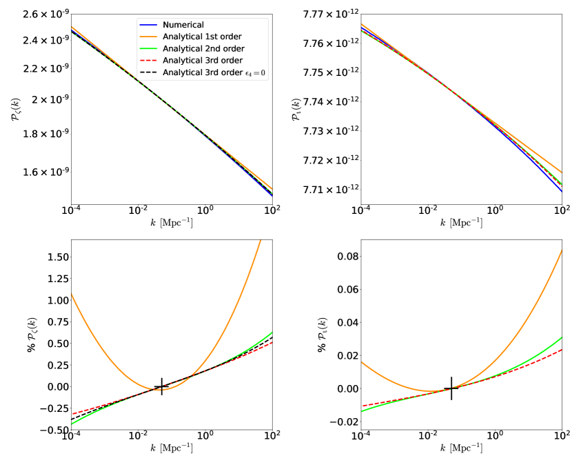
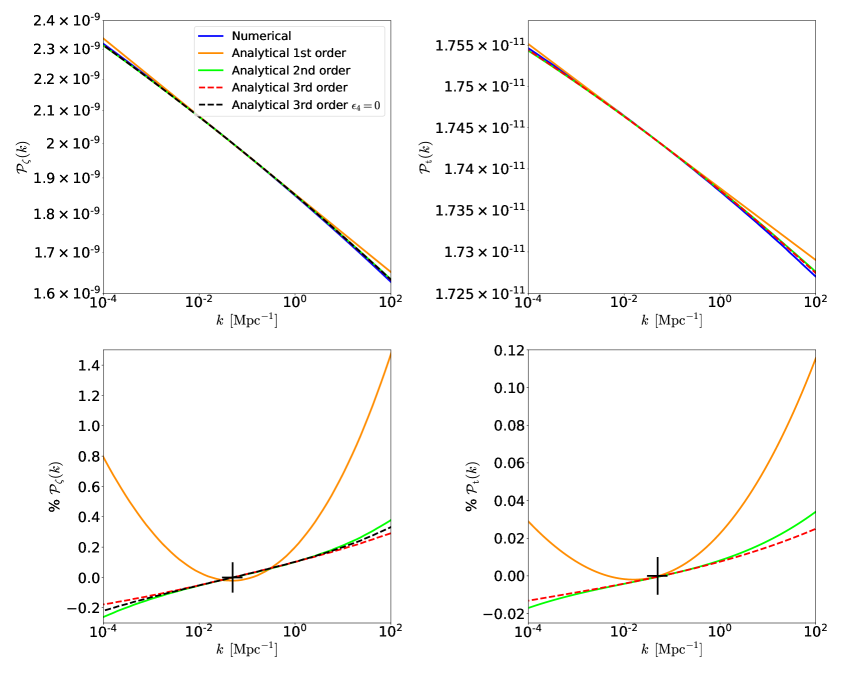
In figs.1 and 2, we present the results for the T-model of -attractor inflation with
, while in figs.3 and 4 we present the results for KKLT inflation with .
We compare the numerical results with respect to the analytical results calculated at first, second, and third-order slow-roll
expansion in the range . Moreover, we also show the comparison for third-order
with . We recall that the amplitudes are normalised in order to obtain the value for the
dimensionless scalar PPS at .
Figure 1: Scalar (left panels) and tensor (right panels) error curves for the T-model -attractor
inflation with . The pivot scale crosses the Hubble horizon 55 e-folds before the end of inflation.
We show on the upper panels the dimensionless PPS and on the lower panels the relative differences of the
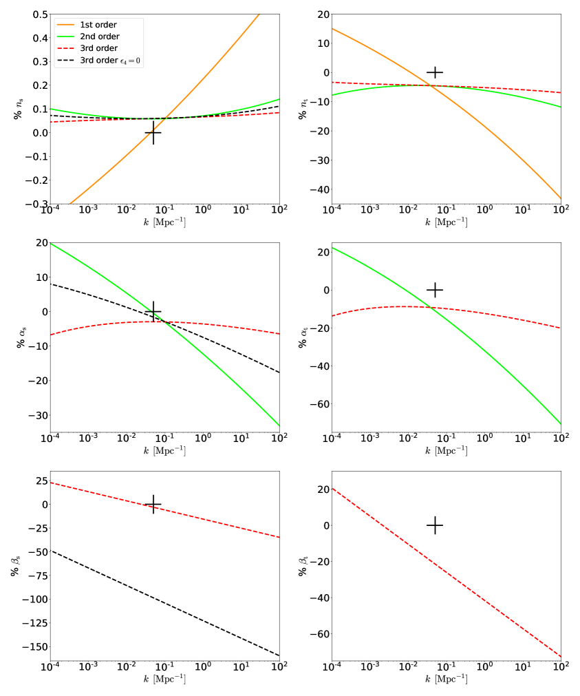
analytic spectra compared to the numerical solution.Figure 2: Relative differences with respect to the numerical solution for the spectral index (upper panels),
running of the spectral index (central panels), and running of the running of the spectral index (lower panels)
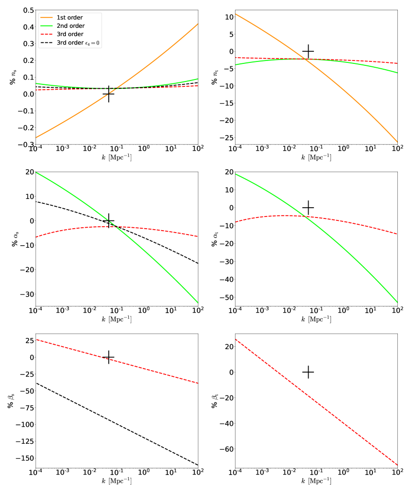
T-model -attractor inflation with .Figure 3: Same as fig.1 but for KKLT inflation for .Figure 4: Same as fig.2 but for KKLT inflation for .
In figs.1 and 3, we present the power spectra comparisons together with the corresponding relative
differences of the analytical results with respect to the numerical solutions. In figs.2 and 4,
we present the relative differences of the spectral indices and , their runnings and , and the runnings of the
running and .
For a certain quantity , where , the
corresponding relative difference is defined as follows
(3.20)
As we can observe in figs.1 and 3, the relative differences on the tensor PPS are one order of
magnitude lower than those of the scalar PPS. We also observe that, on the entire range, the relative errors follow the expected
perturbative hierarchy, i.e. the higher the order, the lower the errors. It is also useful to point out that the third-order case with
acts as a mid-case between the second- and pure third-order. For both models, we observe that around the pivot scale
the second- and third-order PPS relative differences are nearly identical and match the numerical results thanks to the
normalisation performed. Small differences between the second and third order start to appear around of
the order of 0.1% and the curves visibly separate from each other at reaching a maximum difference of
0.5% and 0.3%, for T-model and KKLT inflation respectively. For the tensor PPS, small differences between second and third order
start to arise at , where the relative errors are of the order of 0.01%, and they increase at higher
reaching 0.02% at .
In figs.2 and 4, we present the relative differences for , , and
, for T-model and KKLT inflation, respectively. In general, we find larger differences for the tensor quantities,
however, associated usually to larger observational uncertainties.
For the spectral indexes and , we find that around the pivot scale the relative differences are nearly identical, they
start to differ from . On the other hand, when is lower than the pivot scale, the differences start
to appear from . Including corrections at the second and third order, the relative differences for
in both the models are always at most equal or lower than 0.1%, while for they are always at most equal or lower than
10% (in terms of absolute value). For the runnings of the spectral indexes and , we observe increasing differences between
the second and the third order moving away from the pivot scale; in both cases these differences are always of the order of
around the pivot scale and they increase reaching the order of .
The third-order relative differences for and are consistently around for both the models on the range of
scales probed by CMB measurements; far from the pivot scale the errors are larger. When we consider the case third-order corrections
and , exhibits significantly larger differences compared to the numerical result: these errors start to be
approximately at and increase up to at .
Moreover, we also repeated the comparison for larger values of the inflationary parameters, for T-model inflation and
for KKLT inflation. We observe no significant difference with respect the case presented here for and .
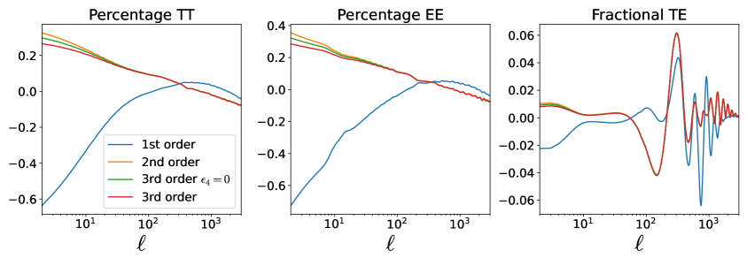
We conclude this section showing in fig.5 the percentage differences on the TT and EE CMB angular power spectra and
the absolute differences on the TE spectrum for T-model -attractor inflation with . The size of the differences
is compatible to the one of the scalar PPS shown in fig.1.
Figure 5: Differences with respect to the numerical solution for the CMB temperature and E-mode polarisation
lensed angular power spectra for the T-model -attractor inflation with .
4 Data Analysis and Cosmological Constraints
In this section, we calculate the uncertainties on the HFFs considering different truncation of the PPS expansion at first
, second , and third order .
We use CosmoMC [53]222https://github.com/cmbant/CosmoMC connected to our modified version
of the code CAMB [54, 55].333https://github.com/cmbant/CAMB
For the Markov chain Monte Carlo (MCMC) analysis, we vary the standard cosmological parameters for a flat CDM
concordance model , , , , and ,444Note that
sampling on the amplitude of the scalar PPS rather that sampling directly on the amplitude
of the scalar field potential allows to overcome some uncertainties on the determination of the end of inflation for which
the slow-roll approximation breaks down; see Ref. [56] for analytic advances. plus the HFFs . We
vary also nuisance and foreground parameters for likelihood considered. We assume two massless neutrino with ,
and a massive one with fixed minimum mass .
We focus our analysis on comparing different cosmological datasets of primary CMB measurements, i.e. temperature and polarisation.
We also consider the case adding non-primary CMB datasets. We therefore consider the following datasets:
•
P18 refers to Planck PR3 primary CMB data [57]. Low-multipole data () consists to the
commander likelihood for temperature and SimAll for the E-mode polarisation. On high multipoles (),
we use the Plik likelihood including CMB temperature up to , E-mode polarisation and
temperature-polarisation cross correlation up to .555https://pla.esac.esa.int/pla/#cosmology
•
ACT refers to ACT DR4 TT, EE, TE power spectra [58, 39] covering the multipole range .
When combining ACT with Planck data we remove temperature data at a certain threshold to avoid for the unaccounted correlation
between the two datasets. We consider two multipole cuts: in the first case we remove Planck data in temperature above
and in the second case we remove ACT data in temperature below .
•
SPT refers to SPT-3G 2018 TT, EE, TE power spectra covering the angular multipole range
[40]. Combining SPT and Planck data we do not consider any cut on the multipole range since data Planck cover a large amount of sky not observed by SPT.
•
BK18 refers B-mode polarisation spectrum for from BICEP2, Keck Array, and BICEP3 observations up to
2018 [41].
•
ext (external) refers to the combination of late-time probes and non-primary CMB data. We include measurements of
baryon acoustic oscillations (BAO) and redshift space distortions (RSD) at low redshift from SDSS-I and -II
sample as Main Galaxy Sample (MGS), BOSS DR12 galaxies over the redshift interval , eBOSS luminous red
galaxies (LRG) and quasars , and Lyman- forest samples [see 59, for details and
references].666https://svn.sdss.org/public/data/eboss/DR16cosmo/tags/v1_0_1/likelihoods/BAO-plus/
We include the Pantheon catalogue of uncalibrated Type Ia Supernovae (SNe) over the redshift range
[60].777https://github.com/dscolnic/Pantheon/ Finally we also include CMB lensing data
from Planck PR3 considering the conservative multipole range [61].
When considering ACT and SPT data not combined with Planck data, we include the Planck low- E-mode polarisation
likelihood SimAll in order to provide information on the optical depth to avoid the use of a Gaussian Planck-inspired
prior on it. We consider P18+BK18, ACT+BK18, SPT+BK18, P18+ACT+BK18, P18+SPT+BK18, and all these combinations also adding the external
datasets.
Mean values and uncertainties on the parameters reported, as well as the contours plotted, have been obtained using GetDist
[62].888https://github.com/cmbant/getdist
Prior ranges on the cosmological parameters are collected on table1. We assume uniform priors an all the HFF parameters
. In Refs. [27, 63] has been sampled with a log-uniform prior corresponding to
sampling the tensor-to-scalar ratio with a logarithmic prior; see Refs. [64, 65] for an extended
discussion on the use of different prior for the tensor-to-scalar ratio.
Parameter
Uniform prior
[0.019, 0.025]
[0.095, 0.145]
[1.03, 1.05]
[0.01, 0.4]
[2.5, 3.7]
[-0.1, 0.1]
[-0.5, 0.5]
[-1, 1]
[-1, 1]
Table 1: Prior ranges for cosmological parameters used in the Bayesian analysis.
4.1 Results
We first present the constraints on slow-roll parameters obtained through the analytic perturbative expansion in terms of the HFFs
for the primordial spectra of cosmological fluctuations during slow-roll inflation. When restricting to first-order
expansion, we obtain
(4.1)
(4.2)
(4.3)
(4.4)
(4.5)
(4.6)
When second-order contributions in the HFFs are included, we obtain
(4.7)
(4.8)
(4.9)
(4.10)
(4.11)
(4.12)
(4.13)
(4.14)
(4.15)
Including third-order contributions in the HFFs, we find close results to the second-order ones with unconstrained,
see table2. The addition of external datasets, which are BAO and RSD measurements, SNe, and CMB lensing, leads to slightly
tighter uncertainties and consistent mean values for and , see table3.
P18 + BK18
ACT + BK18
SPT + BK18
FIRST ORDER
(at 95% CL)
(at 95% CL)
SECOND ORDER
(at 95% CL)
(at 95% CL)
(at 95% CL)
Table 2: Constraints on the main (inflationary related) parameters and derived ones (at 68% CL if not otherwise stated) considering
P18+BK18, ACT+BK18, and SPT+BK18.
P18 + BK18 + ext
ACT + BK18 + ext
SPT + BK18 + ext
FIRST ORDER
(at 95% CL)
(at 95% CL)
SECOND ORDER
(at 95% CL)
(at 95% CL)
(at 95% CL)
Table 3: Same as table2 in combination with the external datasets, which are BAO and RSD measurements, SNe, and CMB
lensing.
The upper limit on , as well as the derived constraint on ( at 95% CL), is almost unchanged among
the different combination of datasets and different truncation being dominated by BK18 data which are always included. On the other
hand, we find different results for and moving from Planck to ACT data. This difference comes from the
almost tension between Planck and ACT data on the inferred value of the scalar spectral index . While the result
from Planck (combining temperature, E-mode polarisation, and lensing) [66] agrees with
the prediction of simplest single-field slow-roll inflationary models, the result from ACT [39] points to
(999Quantified as
;
we perform the analogous estimation for the running of the scalar spectral index .) compatible with a scale invariant
Harrison-Zel’dovich (HZ) primordial power spectrum [67, 68, 69]. We find that Planck ( at 68% CL) and ACT ( at 68% CL) results have a on the inferred
value of when considering primary CMB only at first order in slow-roll expansion, see table2. This number does not
change when the external data are included, see table3.
The discrepancy between Planck and ACT data at the level of scalar PPS parameters persists also when allowing a running of the
scalar spectral index [68, 69]; in our case when we move to the second-order expansion case.
Despite the discrepant results, while Planck is consistent with a zero running at 68% CL
[66] (and with slow-roll single-field inflation predictions, see Ref. [63]), on the contrary ACT
data point to a preference for a positive running [39]. We find a discrepancy on
the inferred value of of with primary CMB alone and in combination with external datasets; larger
numbers compared to the ones obtained considering only second-order terms. We find that Planck ( at
68% CL) and ACT ( at 68% CL) results have a discrepancy on the inferred value of
both considering primary CMB only and in combination with external datasets at second order in slow-roll expansion,
see tables2 and 3.
SPT data agrees with Planck findings but with lager error bars.
4.2 Combined Results
We present here the results for the two combined cases P18+ACT+BK18, assuming two different multiple cut, and the combination
P18+SPT+BK18. When restricting to first-order expansion, we obtain
(4.16)
(4.17)
(4.18)
(4.19)
(4.20)
(4.21)
When second-order contributions in the HFFs are included, we obtain
(4.22)
(4.23)
(4.24)
(4.25)
(4.26)
(4.27)
(4.28)
(4.29)
(4.30)
Also in this case, we find small differences between the second-order and the third-order case and again with
unconstrained, see table4 and table5 for the results including the external datasets. We report the
full results for the third-order case only for the combined datasets with the addition of external data; see table5.
P18 () + ACT
P18 + ACT ()
P18 + SPT
+ BK18
+ BK18
+ BK18
FIRST ORDER
(at 95% CL)
(at 95% CL)
SECOND ORDER
(at 95% CL)
(at 95% CL)
Table 4: Constraints on the main (inflationary related) parameters and derived ones (at 68% CL if not otherwise stated) considering
the combination P18+ACT+BK18 with two different multipole cuts, and P18+SPT-3G+BK18.
P18 () + ACT
P18 + ACT ()
P18 + SPT
+ BK18 + ext
+ BK18 + ext
+ BK18 + ext
FIRST ORDER
(at 95% CL)
(at 95% CL)
SECOND ORDER
(at 95% CL)
(at 95% CL)
THIRD ORDER
(at 95% CL)
(at 95% CL)
Table 5: Same as table4 in combination with the external datasets, which are BAO and RSD measurements, SNe, and CMB
lensing.
The combination P18+ACT is closer to the Planck alone results for both the two multipole cut applied in temperature. While the
case with the cut on ACT data, with , at 68% CL () agrees well
with Planck results, the case cutting Planck temperature data, with , gives
at 68% CL () when considering primary CMB only; we find and
including second-order corrections, respectively.
Results for the scalar running for which the combination P18+ACT with are loser to the constraints
obtained with Planck data alone; we find with the cut on ACT data and
by cutting Planck data, both at 68% CL.
The combination P18+SPT agrees with Planck findings but with tighter error bars.
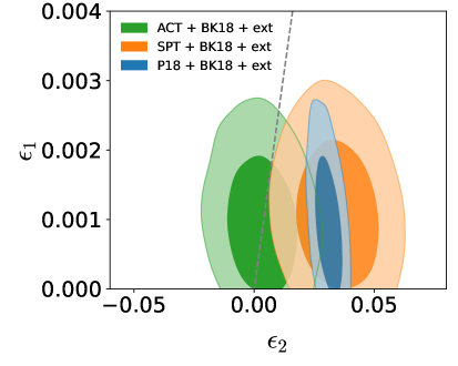
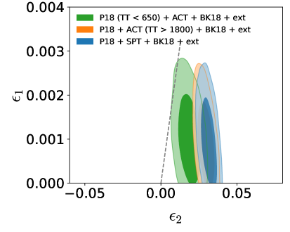
In fig.6, we show the 68% CL and 95% CL of the HFFs obtained for the first-order analysis both for Planck, ACT, and
SPT alone and their combinations. Our findings are consistent with the global picture that CMB data prefer potentials which are
concave, i.e. , in the observable window, with exception of the ACT+BK18 case.
Figure 6: Marginalised joint confidence contours for the first two HFF parameters and assuming first-order
slow-roll predictions. The grey dashed line divide the parameter space from convex (left side) to concave (right side) single-field
slow-roll potentials.
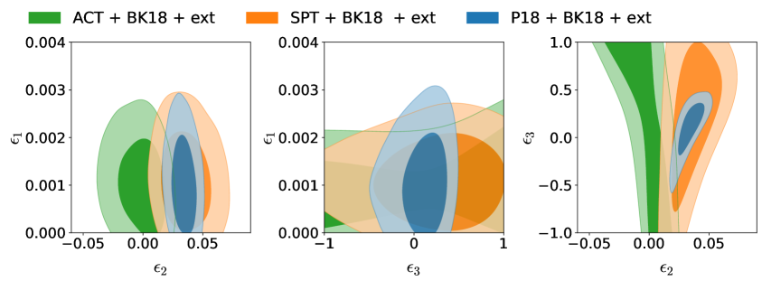
In fig.7, we show the 68% CL and 95% CL of the HFFs obtained for the second-order analysis both for Planck, ACT, and
SPT alone on the left and their combinations on the right.
Figure 7: Marginalised joint confidence contours for the first two HFF parameters , , and assuming
second-order slow-roll predictions.
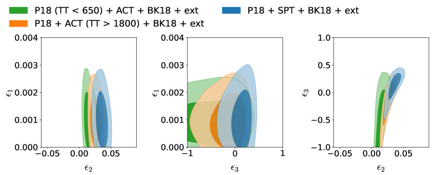
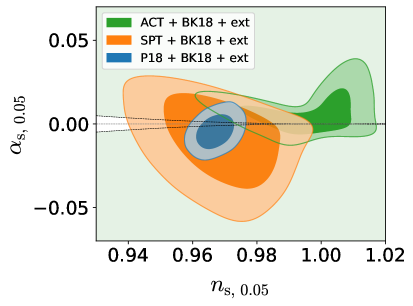
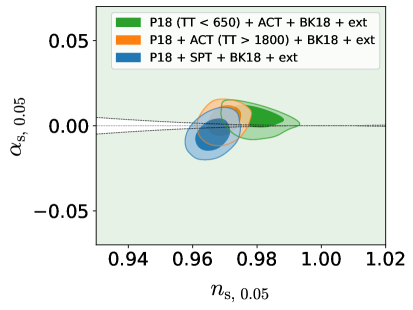
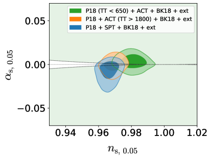
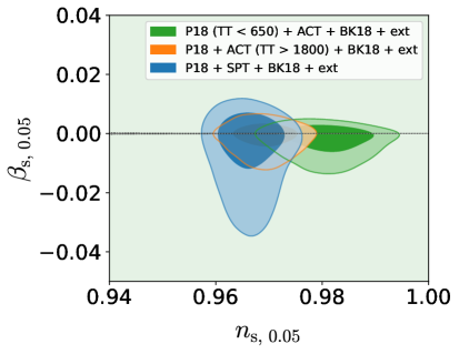
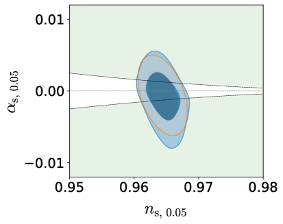
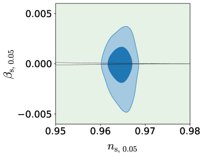
Finally, we show the 68% CL and 95% CL marginalised constraints on the scalar inflationary parameters, derived
using eqs.C.20, C.21 and C.22, that are for the second-order HFF expansion the scalar spectral index and its running
in fig.8 while for the third-order expansion include also the running of the running of the scalar spectral
index , see fig.8.
Although current constraints are consistent with small values for , , and as predicted by single-field slow-roll
inflationary models, much larger values are still allowed by current CMB measurements. Here the light shaded region corresponds to
for which we have qualitatively violation of the single-field slow-roll predictions and analogously
.
Figure 8: Marginalised joint confidence contours for the scalar spectral index and its running assuming second-order
slow-roll predictions (upper panels) and for the scalar spectral index , its running , and the running of the running
assuming third-order slow-roll predictions (lower panels).
4.3 Future CMB Constraints
In this subsection, we explore the forecasted capabilities of a concept for a future CMB space mission. Assuming that CMB
anisotropies follow a Gaussian distribution and are statistically isotropic, we use the following Gaussian likelihood
[70, 71]
(4.31)
where denote the theoretical data covariance matrices
(4.32)
and are the fiducial data covariance matrices
(4.33)
Noise power spectra for the temperature and polarisation angular power spectra account for isotropic noise deconvolved with the
instrumental Gaussian beam as
(4.34)
We assume an effective noise variance and
and an effective beam resolution of
over 70% of the sky considering the multipole range . These
instrumental specifications corresponds to a CMB experiment cosmic-variance limited up to in temperature,
in E-mode polarisation, and in the gravitational lensing over almost the full sky.
Together with the primary temperature and polarisation anisotropy signal, we also take into account information from CMB weak
lensing, considering the power spectrum of the CMB lensing potential . For the CMB lensing noise power spectrum,
we adopt the minimum-variance quadratic estimator for the lensing reconstruction [72] in the range
, combining the TT, EE, BB, TE, TB, and EB estimators and applying iterative lensing reconstruction
according to Refs. [73, 74].
Finally, we consider internal delensing [75, 76, 77], with the above
specifications, of the B-mode angular power spectrum in order to reduce the non-primordial contribution induced by lensing.
We implement the delensing removing the lensing contribution to the B-mode angular power spectra and adding an error contribution
to the instrumental noise .
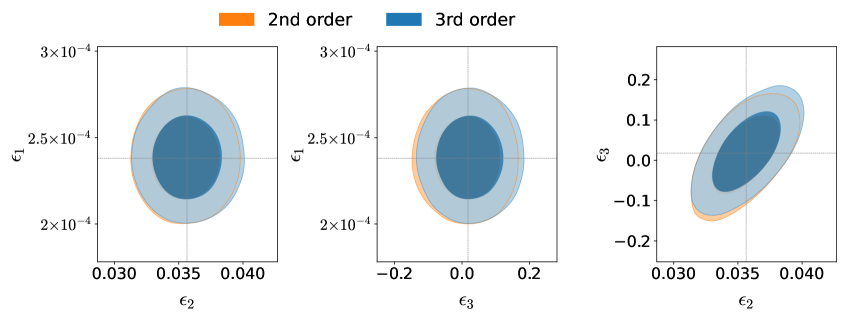
Figure 9: Marginalised joint confidence contours for the first two HFF parameters , , and
assuming second-and third-order slow-roll predictions (upper panels). Marginalised joint confidence contours for the scalar spectral
index and its running assuming second- and third-order slow-roll predictions (lower left panel) and for the scalar
spectral index , its running of the running assuming third-order slow-roll predictions (lower right
panel).
We assume a flat Universe with a cosmological constant, two massless neutrino with , and a massive one with
fixed minimum mass . To generate the fiducial angular power spectra, we have fixed the HFFs to the
expected numbers for T-model of -attractor inflation with assuming at .
This corresponds to , , , and .
On these simulated measurements, we analyse the PPS equations at second order, with and no correction at third
order, and the full third-order expressions. The results are shown in fig.9. We conclude that for a futuristic
CMB experiment alone:
•
HFFs are well recovered without any bias or significant change in the uncertainties stopping at second order;
•
the fourth HFF remains unconstrained;
•
uncertainties on the HFFs are significantly reduced with a high significance statistical detection of
(for this specific fiducial also is well measured). For these case, we obtain
, , and at 68% CL consistently with Ref. [78].
5 Conclusions
In this paper, we conducted an extensive analysis of the primordial power spectra (PPS) for both scalar and tensor perturbations,
focusing on the higher-order corrections within the slow-roll inflationary framework. By utilising Green’s function techniques to
solve the Mukhanov-Sasaki equation and its tensor counterpart, we were able to extend our analytical calculations up to third-order
corrections, thereby refining the perturbative expansion in terms of slow-roll parameters.
Our results demonstrate that higher-order corrections significantly enhance the accuracy of the predicted power spectra, spectral
indices, and their derivatives. However going from the second to the third-order expansion, the improvement becomes appreciable at
very small scales leaving almost unaffected the CMB angular power spectra,
see figs.1, 2, 3 and 4.
Since the accuracy requirement for tensor quantities is less than on the scalars, it is the scalars upon which attention should be
focused.
We investigated the constraints on the first four HFFs obtained from CMB anisotropy measurements in combination with late-time
cosmological observations such as uncalibrated Type Ia Supernovae from the Pantheon catalogue, baryon acoustic oscillations and
redshift space distortions from SDSS/BOSS/eBOSS.
Regarding the CMB datasets considered, we study the impact of different combination of temperature and E-mode polarisation data from
Planck, ACT, and SPT. We always included in our analysis B-mode polarisation measurements from BICEP/Keck. Our analysis yields a
stringent upper limit for the first HFF, at 95% CL, primarily constrained by BICEP/Keck data. This
result underscores the robustness of across various combinations of observational datasets. By combining data from
Planck with late-time cosmological observations, we derived at 68% CL when considering only
first-order corrections. Including second- and third-order corrections broadens this constraint to
at 68% CL. For the third HFF, our findings indicate a value of at 95% CL, which remains consistent
across second- and third-order corrections. The fourth HFF , however, remains unconstrained by current data as shown also
in Ref. [28].
We then add small scale CMB measurements from ACT and SPT to the Planck data. Our combination of Planck data with measurements
from ACT (were we removed the temperature data below as recommended from the ACT collaboration to avoid correlations
between the two datasets) and from SPT led to consistent results with slightly more stringent constraints on and
. ACT data alone results and the combination of ACT with Planck temperature data removed above , lead to
shifts in the mean values of and , which suggest a preference for higher values of the scalar spectral index
and positive values for the running of the scalar spectral index.
We studied the case of a futuristic CMB experiments with realistic and almost cosmic-variance limited specifications.
These results show that second-order equations are accurate enough to describe slow-roll physics, see fig.9.
remains unconstrained also for future CMB measurements.
In conclusion, future small-scale CMB measurements from ACT, SPT, and Simons Observatory will be crucial to further test high-order
terms in the slow-roll expansion and the validity of slow-roll inflation. In addition, future data over a wider range of scales such
as large-scale structure (LSS) measurements from Euclid [79], CMB spectral distorsions [80],
21 cm experiments [81], and on smaller scales abundance of primordial black holes can offer useful constraints on the
primordial curvature power spectrum [82]. These additional cosmological probes will enable us to confirm
slow-roll inflation, for instance through a detection of the running of the scalar spectral index
[79, 83, 84], or to falsify it.
Acknowledgments
MB and SSS acknowledge financial support from the INFN InDark initiative.
MB also acknowledges financial support from the COSMOS network (www.cosmosnet.it) through the ASI (Italian Space Agency)
Grants 2016-24-H.0, 2016-24-H.1-2018, 2020-9-HH.0 (participation in LiteBIRD phase A) and by “Bando Giovani anno 2023 per
progetti di ricerca finanziati con il contributo 5x1000 anno 2021”.
SSS acknowledges that this publication was produced while attending the PhD program in Space Science and Technology at the University of Trento, Cycle XXXVIII, with the support of a scholarship co-financed by the Ministerial Decree no. 351 of 9th April 2022, based on the NRRP - funded by the European Union - NextGenerationEU - Mission 4 ”Education and Research”, Component 2 ”From Research to Business”, Investment 3.3. SSS acknowledges that this article/publication is based upon work from COST Action CA21136 – “Addressing observational tensions in cosmology with systematics and fundamental physics (CosmoVerse)”, supported by COST (European Cooperation in Science and Technology).
Appendix A Useful Integrals
Here some useful integrals used to manipulate the solutions entering in the third-order Green’s function solution eq.2.27.
(A.1a)
(A.1b)
(A.1c)
(A.2a)
(A.2b)
(A.2c)
(A.3a)
(A.3b)
(A.3c)
(A.4a)
(A.4b)
(A.5a)
(A.5b)
(A.5c)
(A.6a)
(A.6b)
(A.6c)
(A.7a)
(A.7b)
(A.7c)
(A.8a)
(A.8b)
(A.9a)
(A.9b)
(A.9c)
(A.10a)
(A.10b)
(A.11a)
(A.11b)
(A.11c)
Appendix B Super-Hubble Limits for the Integrals
We report here the asymptotic solutions, calculated in the super-Hubble limit, of the integrals appearing
in eqs.2.28, 2.30a, 2.30b, 2.33, 2.36 and 2.38 required to compute the primordial power spectra of scalar and
tensor perturbations.
(B.1)
(B.2)
(B.3)
(B.4)
(B.5)
(B.6)
Appendix C Parameterisation of the Power Spectra
The power spectra of scalar and tensor perturbations can be estimated through analytical methods. Typically, this involves expanding
the power spectra around a specific wavenumber, denoted as , and then determining the coefficients through a slow-roll expansion
or another suitable approximation technique. Because the analysis must span multiple orders of magnitude in , the most effective
expansion variable is . In this regard, two expansions have been proposed in the literature [20]. The first one
consists in expanding directly the power spectrum in , leading to
(C.1)
where and
(C.2)
Therefore, the coefficients and at third order are respectively
(C.3)
(C.4)
(C.5)
(C.6)
(C.7)
(C.8)
(C.9)
(C.10)
Alternatively, it is possible to expand the logarithm of the power spectrum in as
(C.11)
and the coefficients and at third order are respectively
(C.12)
(C.13)
(C.14)
(C.15)
(C.16)
(C.17)
(C.18)
(C.19)
Using the latter parameterisation, it is possible to write both the scalar and tensor spectral indices, runnings, and runnings of
the running with respect to the coefficients as follows
(C.20)
(C.21)
(C.22)
(C.23)
(C.24)
(C.25)
References
[1]
A.A. Starobinsky, A new type of isotropic cosmological models without singularity, Physics Letters B91 (1980) 99.
[2]
A.H. Guth, Inflationary universe: A possible solution to the horizon and flatness problems, Phys. Rev. D23 (1981) 347.
[3]
A.D. Linde, A new inflationary universe scenario: A possible solution of the horizon, flatness, homogeneity, isotropy and primordial monopole problems, Physics Letters B108 (1982) 389.
[4]
A. Albrecht and P.J. Steinhardt, Cosmology for Grand Unified Theories with Radiatively Induced Symmetry Breaking, Phys. Rev. Lett.48 (1982) 1220.
[5]
S.W. Hawking, I.G. Moss and J.M. Stewart, Bubble collisions in the very early universe, Phys. Rev. D26 (1982) 2681.
[7]
V.F. Mukhanov, Gravitational instability of the universe filled with a scalar field, Soviet Journal of Experimental and Theoretical Physics Letters41 (1985) 493.
[9]
Planck Collaboration, P.A.R. Ade, N. Aghanim, C. Armitage-Caplan, M. Arnaud, M. Ashdown et al., Planck 2013 results. XXII. Constraints on inflation, A&A571 (2014) A22 [1303.5082].
[10]
Planck Collaboration, P.A.R. Ade, N. Aghanim, M. Arnaud, F. Arroja, M. Ashdown et al., Planck 2015 results. XX. Constraints on inflation, A&A594 (2016) A20 [1502.02114].
[11]
Planck Collaboration, Y. Akrami, F. Arroja, M. Ashdown, J. Aumont, C. Baccigalupi et al., Planck 2018 results. X. Constraints on inflation, A&A641 (2020) A10 [1807.06211].
[13]
A.A. Starobinskiǐ, Spectrum of relict gravitational radiation and the early state of the universe, Soviet Journal of Experimental and Theoretical Physics Letters30 (1979) 682.
[14]
V.F. Mukhanov, Quantum theory of gauge-invariant cosmological perturbations, Soviet Journal of Experimental and Theoretical Physics67 (1988) 1297.
[15]
E.D. Stewart and D.H. Lyth, A more accurate analytic calculation of the spectrum of cosmological perturbations produced during inflation, Physics Letters B302 (1993) 171 [gr-qc/9302019].
[17]
T.T. Nakamura and E.D. Stewart, The spectrum of cosmological perturbations produced by a multi-component inflaton to second order in the slow-roll approximation, Physics Letters B381 (1996) 413 [astro-ph/9604103].
[31]
K. Abazajian, G. Addison, P. Adshead, Z. Ahmed, S.W. Allen, D. Alonso et al., CMB-S4 Science Case, Reference Design, and Project Plan, arXiv e-prints (2019) arXiv:1907.04473 [1907.04473].
[32]
K. Abazajian, G.E. Addison, P. Adshead, Z. Ahmed, D. Akerib, A. Ali et al., CMB-S4: Forecasting Constraints on Primordial Gravitational Waves, ApJ926 (2022) 54 [2008.12619].
[35]
L. Amendola, S. Appleby, A. Avgoustidis, D. Bacon, T. Baker, M. Baldi et al., Cosmology and fundamental physics with the Euclid satellite, Living Reviews in Relativity21 (2018) 2 [1606.00180].
[36]
Euclid Collaboration, A. Blanchard, S. Camera, C. Carbone, V.F. Cardone, S. Casas et al., Euclid preparation. VII. Forecast validation for Euclid cosmological probes, A&A642 (2020) A191 [1910.09273].
[37]
Euclid Collaboration, S. Ilić, N. Aghanim, C. Baccigalupi, J.R. Bermejo-Climent, G. Fabbian et al., Euclid preparation. XV. Forecasting cosmological constraints for the Euclid and CMB joint analysis, A&A657 (2022) A91 [2106.08346].
[38]
Planck Collaboration, N. Aghanim, Y. Akrami, F. Arroja, M. Ashdown, J. Aumont et al., Planck 2018 results. I. Overview and the cosmological legacy of Planck, A&A641 (2020) A1 [1807.06205].
[40]
L. Balkenhol, D. Dutcher, A. Spurio Mancini, A. Doussot, K. Benabed, S. Galli et al., Measurement of the CMB temperature power spectrum and constraints on cosmology from the SPT-3G 2018 T T , T E , and E E dataset, Phys. Rev. D108 (2023) 023510 [2212.05642].
[41]
P.A.R. Ade, Z. Ahmed, M. Amiri, D. Barkats, R.B. Thakur, C.A. Bischoff et al., Improved Constraints on Primordial Gravitational Waves using Planck, WMAP, and BICEP/Keck Observations through the 2018 Observing Season, Phys. Rev. Lett.127 (2021) 151301 [2110.00483].
[42]
V.F. Mukhanov and G.V. Chibisov, Quantum fluctuations and a nonsingular universe, Soviet Journal of Experimental and Theoretical Physics Letters33 (1981) 532.
[54]
A. Lewis, A. Challinor and A. Lasenby, Efficient Computation of Cosmic Microwave Background Anisotropies in Closed Friedmann-Robertson-Walker Models, ApJ538 (2000) 473 [astro-ph/9911177].
[57]
Planck Collaboration, N. Aghanim, Y. Akrami, M. Ashdown, J. Aumont, C. Baccigalupi et al., Planck 2018 results. V. CMB power spectra and likelihoods, A&A641 (2020) A5 [1907.12875].
[58]
S.K. Choi, M. Hasselfield, S.-P.P. Ho, B. Koopman, M. Lungu, M.H. Abitbol et al., The Atacama Cosmology Telescope: a measurement of the Cosmic Microwave Background power spectra at 98 and 150 GHz, J. Cosmology Astropart. Phys.2020 (2020) 045 [2007.07289].
[59]
S. Alam, M. Aubert, S. Avila, C. Balland, J.E. Bautista, M.A. Bershady et al., Completed SDSS-IV extended Baryon Oscillation Spectroscopic Survey: Cosmological implications from two decades of spectroscopic surveys at the Apache Point Observatory, Phys. Rev. D103 (2021) 083533 [2007.08991].
[60]
D.M. Scolnic, D.O. Jones, A. Rest, Y.C. Pan, R. Chornock, R.J. Foley et al., The Complete Light-curve Sample of Spectroscopically Confirmed SNe Ia from Pan-STARRS1 and Cosmological Constraints from the Combined Pantheon Sample, ApJ859 (2018) 101 [1710.00845].
[61]
Planck Collaboration, N. Aghanim, Y. Akrami, M. Ashdown, J. Aumont, C. Baccigalupi et al., Planck 2018 results. VIII. Gravitational lensing, A&A641 (2020) A8 [1807.06210].
[64]
L.T. Hergt, W.J. Handley, M.P. Hobson and A.N. Lasenby, Bayesian evidence for the tensor-to-scalar ratio and neutrino masses : Effects of uniform vs logarithmic priors, Phys. Rev. D103 (2021) 123511 [2102.11511].
[65]
G. Galloni, S. Henrot-Versillé and M. Tristram, Robust constraints on tensor perturbations from cosmological data: a comparative analysis from Bayesian and frequentist perspectives, arXiv e-prints (2024) arXiv:2405.04455 [2405.04455].
[66]
Planck Collaboration, N. Aghanim, Y. Akrami, M. Ashdown, J. Aumont, C. Baccigalupi et al., Planck 2018 results. VI. Cosmological parameters, A&A641 (2020) A6 [1807.06209].
[67]
J.-Q. Jiang and Y.-S. Piao, Toward early dark energy and ns=1 with P l a n c k , ACT, and SPT observations, Phys. Rev. D105 (2022) 103514 [2202.13379].
[68]
E. Di Valentino, W. Giarè, A. Melchiorri and J. Silk, Quantifying the global ’CMB tension’ between the Atacama Cosmology Telescope and the Planck satellite in extended models of cosmology, MNRAS520 (2023) 210 [2209.14054].
[69]
W. Giarè, F. Renzi, O. Mena, E. Di Valentino and A. Melchiorri, Is the Harrison-Zel’dovich spectrum coming back? ACT preference for ns 1 and its discordance with Planck, MNRAS521 (2023) 2911 [2210.09018].
[76]
M. Kesden, A. Cooray and M. Kamionkowski, Separation of Gravitational-Wave and Cosmic-Shear Contributions to Cosmic Microwave Background Polarization, Phys. Rev. Lett.89 (2002) 011304 [astro-ph/0202434].
[80]
G. Cabass, E. Di Valentino, A. Melchiorri, E. Pajer and J. Silk, Constraints on the running of the running of the scalar tilt from CMB anisotropies and spectral distortions, Phys. Rev. D94 (2016) 023523 [1605.00209].
[82]
G. Sato-Polito, E.D. Kovetz and M. Kamionkowski, Constraints on the primordial curvature power spectrum from primordial black holes, Phys. Rev. D100 (2019) 063521 [1904.10971].
[83]
B. Bahr-Kalus, D. Parkinson and R. Easther, Constraining cosmic inflation with observations: Prospects for 2030, MNRAS520 (2023) 2405 [2212.04115].
[84]
R. Easther, B. Bahr-Kalus and D. Parkinson, Running primordial perturbations: Inflationary dynamics and observational constraints, Phys. Rev. D106 (2022) L061301 [2112.10922].