$SL(2,\mathbb{Z})$ Cosmological Attractors

Abstract

We study cosmological theory where the kinetic term and potential have $SL(2,\mathbb{Z})$ symmetry. Potentials have a plateau at large values of the inflaton field where the axion forms a flat direction, a saddle point at $\tau=i$, and a minimum at $\tau=e^{2\pi i\over 3}$. Due to the underlying hyperbolic geometry, the theory exhibits an $\alpha$-attractor behavior: its cosmological predictions are stable with respect to certain modifications of the $SL(2,\mathbb{Z})$ invariant potentials. We present a supersymmetric version of this theory in the framework of $\overline{D3}$ induced geometric inflation. The choice of $\alpha$ is determined by underlying string compactification. For example, in a CY compactification with $T^{2}$, one has $3\alpha=1$, the lowest discrete Poincaré disk target for LiteBIRD.

1 Introduction

It was proposed in Casas:2024jbw to approach inflationary cosmology from the quantum gravity/string theory perspective and view the modular invariant effective potential $V(\tau,\bar{\tau})$ as the one which already includes all relevant corrections such as higher powers of the curvature corrections to the action. The proposal also includes a requirement that the modular invariant effective potential $V(\tau,\bar{\tau})$ as a function of large ${\rm Im}(\tau)$ has a plateau so that a long period of inflation is possible in agreement with the cosmological observations.

Here we will construct general $SL(2,\mathbb{Z})$ invariant theories and study their cosmological properties. They depend on a single complex field $\tau=\tau_{1}+i\tau_{2}$

$${{\cal L}(\tau,\bar{\tau})\over\sqrt{-g}}={R\over 2}+{3\alpha\over 4}\,{\partial\tau\partial\bar{\tau}\over({\rm Im}\tau)^{2}}-V(\tau,\bar{\tau})$$ (1)

The scalar kinetic term has an unbroken $SL(2,\mathbb{R})$ symmetry whereas the potential breaks it to $SL(2,\mathbb{Z})$ symmetry. The questions we would like to address here are:

1. Is this kinetic term unique as long as we request only $SL(2,\mathbb{Z})$ symmetry, i.e. we allow $SL(2,\mathbb{R})$ of the scalar kinetic term to be broken to $SL(2,\mathbb{Z})$?

2. What kind of potentials with $SL(2,\mathbb{Z})$ symmetry are possible, and under what conditions do they agree with the cosmological observations?

We will give examples of such potentials and will find that the relevant cosmological models have features closely related to cosmological $\alpha$-attractor models introduced earlier Kallosh:2013yoa ; Galante:2014ifa ; Kallosh:2015zsa . $SL(2,\mathbb{R})$ symmetry of the kinetic terms of the cosmological $\alpha$-attractor models was discussed in details in Kallosh:2013yoa ; Galante:2014ifa ; Kallosh:2015zsa ; Carrasco:2015uma ; Carrasco:2015rva ; Carrasco:2015pla both in half-plane variables $\tau$ as well as in disk variables $z={\tau-i\over\tau+i}$. Their specific features related to hyperbolic geometry were described in Achucarro:2017ing ; Linde:2018hmx where it was found that even if the axion, the superpartner of the inflaton, is light, it effectively freezes during inflation and is not harmful for successful inflation. This freezing is due to the kinetic term of the axion is hyperbolic geometry

$${3\alpha\over 4}\,{\partial\tau\partial\bar{\tau}\over({\rm Im}\tau)^{2}}=-{1\over 2}(\partial\varphi)^{2}-{3\alpha\over 4}e^{2\sqrt{2\over 3\alpha}\varphi}(\partial\theta)^{2}$$ (2)

In evolution equations one finds that during inflation $\dot{\theta}$ is suppressed with respect to $\dot{\varphi}$ by the factor of $e^{-\sqrt{2\over 3\alpha}\,\varphi}$.

The supersymmetric version of the $SL(2,\mathbb{R})$ symmetric models (1) will be given in the framework of $\overline{D3}$-induced geometric inflation Kallosh:2017wnt ; McDonough:2016der which depends on superpotential, on Kähler potential and on a new real function which is a moduli dependent metric of the nilpotent superfield $X$

$$W(\tau)\,,\qquad K(\tau,\bar{\tau})\,,\qquad G_{X\bar{X}}(\tau,\bar{\tau})\ .$$ (3)

The nilpotent superfield $X^{2}=0$ represents the upliting effect of $\overline{D3}$ brane in supergravity. Our new models are defined by a choice of $SL(2,\mathbb{Z})$ invariant new function $G_{X\bar{X}}(\tau,\bar{\tau})$. In the language of the “liberated supergravity” Farakos:2018sgq , supergravity potential includes a new arbitrary function in addition to F- and D-terms potentials so that ${\cal V}_{lib}={\cal V}_{F}+{\cal V}_{D}+{\cal U}(\tau,\bar{\tau})$ and $G^{X\bar{X}}(\tau,\bar{\tau})=e^{-K}{\cal U}(\tau,\bar{\tau})$, under certain conditions. This new function is also related to the metric of the nilpotent superfield. In our new cosmological models, we take this additional function describing the potential to be an $SL(2,\mathbb{Z})$ invariant.

Thus, we will describe supersymmetric $SL(2,\mathbb{Z})$ models where the light axion is frozen in hyperbolic geometry, as in models studied in Achucarro:2017ing ; Linde:2018hmx .

The importance of these new cosmological models is that they are relevant to the targets for the CMB future LiteBIRD experiment LiteBIRD:2022cnt , known as Poincaré disks Ferrara:2016fwe ; Kallosh:2021vcf , see Fig. 2 in LiteBIRD:2022cnt . These are $\alpha$-attractors with integer values of $3\alpha=1,2,3,4,5,6,7$. The new $SL(2,\mathbb{Z})$ invariant models under certain conditions give the same predictions as the models with Poincaré disks.

2 Warm up: $\alpha$-attractor models

Consider the following theory

$${{\cal L}\over\sqrt{-g}}={R\over 2}-{3\alpha\over 4}\,{(\partial\rho)^{2}\over\rho^{2}}-V(\rho)\ .$$ (4)

where the potentials $V(\rho)$ are non-singular near the pole at $\rho=0$, and can be expanded in series

$$V=V_{0}\left(1-c\rho+{\cal O}(\rho^{2})\right)$$ (5)

with $c>0$. Since the kinetic term is invariant with respect to the rescaling of $\rho$, one can replace $\rho\to\rho/c$. In these rescaled variables, the potential in the vicinity of the pole acquires the universal form

$$V=V_{0}(1-\rho+\cdots)$$ (6)

assuming that $\rho^{n}$ with $n\geq 2$ can be neglected. One can represent ${\cal L}$ in canonical variables $\varphi$, where $\rho=e^{-\sqrt{2\over 3\alpha}\,\varphi}$. This yields

$${{\cal L}\over\sqrt{-g}}={R\over 2}-{1\over 2}(\partial\varphi)^{2}-V(e^{-\sqrt{2\over 3\alpha}\varphi}).$$ (7)

At large values of $\varphi$, such that $e^{-\sqrt{2\over 3\alpha}\varphi}\ll 1$, the potential is

$$V=V_{0}\left(1-e^{-\sqrt{2\over 3\alpha}\varphi}+{\cal O}(e^{-2\sqrt{2\over 3\alpha}\varphi})\right)\ .$$ (8)

During inflation at $\varphi\gg\sqrt{3\alpha\over 2}$ the potential is determined by the first two terms in the expansion, containing only two parameters, $V_{0}$ and $\alpha$. In this approximation, one can calculate the total expansion of the universe $e^{N_{e}}$ during inflation when the field rolls down from $\varphi=\varphi_{N_{e}}$:

$$e^{-\sqrt{2\over 3\alpha}\varphi_{N}}={3\alpha\over 8N_{e}}.$$ (9)

Therefore, the amplitude of inflationary perturbations generated at large values of the field $\varphi$ corresponding to $N_{e}\sim 55$ and $\alpha\lesssim O(1)$ does not depend on higher order terms in the expansion (8). In particular, the amplitude of inflationary perturbations $A_{s}$, the spectral index $n_{s}$, and the tensor to scalar ratio $r$ in the large $N_{e}$ limit are given by Kallosh:2013yoa ; Galante:2014ifa ; Kallosh:2021mnu

$$A_{s}={V_{0}\,N_{e}^{2}\over 18\pi^{2}\alpha}\ ,\qquad n_{s}=1-{2\over N_{e}}\ ,\qquad r={12\alpha\over N^{2}_{e}}\ .$$ (10)

Since these predictions depend only on $V_{0}$ and $\alpha$ and do not depend on many other features of the original potential $V(\rho)$, we called these models $\alpha$-attractors.

Some of the simplest $\alpha$-attractor potentials are E-models

$$V=V_{0}\left(1-\rho\right)^{2n}=V_{0}\left(1-e^{-\sqrt{2\over 3\alpha}\varphi}\right)^{2n}\$$ (11)

These potentials have an inflationary plateau at $\varphi\gg\sqrt{3\alpha\over 2}$, and they blow up at large negative values of $\varphi$. For $n=1$ and $\alpha=1$ the potential (LABEL:EE) coincides with the potential of the Starobinsky model. In general, $\alpha$ can take any value, which allows to describe observational data with any $r$, all the way down to zero. On the other hand, in models based on maximal supergravity, $3\alpha$ may take 7 integer values, $3\alpha=1,2,...,7$ Ferrara:2016fwe ; Kallosh:2021vcf .

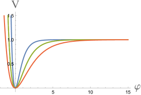
Figure 1: E-model potential (LABEL:EE) for $V_{0}=1$, $n=1$, $3\alpha=1$ (blue line), $3\alpha=3$ (green line, Starobinsky model), and $3\alpha=7$ (red line). The potential blows up at large negative values of $\varphi$ and has a plateau at large positive $\varphi$.

As a preview to $SL(2,\mathbb{Z})$ cosmological $\alpha$-attractors consider the T-models with the potential

$$V=V_{0}\left({1-\rho\over 1+\rho}\right)^{2n}=V_{0}\tanh^{2n}{\varphi\over\sqrt{6\alpha}}\ .$$ (12)

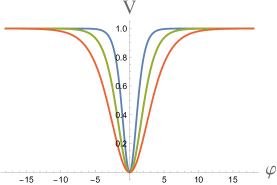
Figure 2: T-model potential (12) for $V_{0}=1$, $3\alpha=1$ (blue line), $3\alpha=3$ (green line), and $3\alpha=7$ (red line).

This potential has the expansion

$$V=V_{0}(1-4n\rho+{\cal O}(\rho^{2}))$$ (13)

near the pole at $\rho=0$. Thus this model belongs to the general class of $\alpha$-attractors and has the same cosmological predictions for $N_{e}\gg 1$ and $\alpha\lesssim O(5)$ as the ones in eq. (10). These predictions depend only on $V_{0}$ and $\alpha$.

The theory (4) with this potential has the inversion symmetry

$$\rho\to\rho^{-1}\,,\qquad\varphi\to-\varphi$$ (14)

Therefore the potential of this model (12) looks like letter T: It has two symmetric plateaus, shoulders of the same height at $|\varphi|\gg\sqrt{3\alpha\over 2}$. These versions of $\alpha$-attractors are called T-models Kallosh:2013hoa ; Kallosh:2013yoa . We show these potential for $V_{0}=1$ and $3\alpha=1,3,7$ in Fig. 2. Cosmological predictions of these models are compatible with all presently available CMB-related observational data for $\alpha\lesssim O(5)$ Kallosh:2021mnu , see Fig. 3.

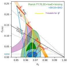
Figure 3: The figure shows the main results of the BICEP/Keck BICEPKeck:2021gln superimposed with the predictions of $\alpha$-attractor T-models with the potential $\tanh^{2n}{\varphi\over\sqrt{6\alpha}}$ Kallosh:2013yoa ; Kallosh:2015zsa ; Kallosh:2021mnu . At $\alpha\gg 1$, these models have different predictions corresponding to different potentials $\phi^{n}$ (at $\alpha\rightarrow\infty$), but with a decrease of $\alpha$, these predictions converge in the dark blue area favored by CMB observations.

3 Symmetries: $SL(2,\mathbb{R})$ and $SL(2,\mathbb{Z})$

Here we study the action in eq. (1) which depends on modulus $\tau(x)$ where the field $\tau$ is defined in Poincaré upper half-plane such that

$${\cal H}=\{\tau\in\mathbb{C},{\rm Im}\,\tau>0\}$$ (15)

and $\tau=\tau_{1}+i\tau_{2}$ is a complex modulus. A kinetic term for scalar fields $\tau$ in eq. (1) of the form ${\partial\tau\partial\bar{\tau}\over({\rm Im}\tau)^{2}}$, has an $SL(2,\mathbb{R})$ symmetry. The action of $SL(2,\mathbb{R})$ maps the upper half-plane to itself and

$$(\Gamma\cdot\tau)\equiv\frac{a\tau+b}{c\tau+d},\quad{\rm where}\,\,\Gamma=\begin{pmatrix}a&b\\ c&d\end{pmatrix}\,,\quad\det\Gamma=ad-cb=1$$ (16)

All parameters $a,b,c,d$ of $SL(2,\mathbb{R})$ symmetry are real numbers. The symmetries can be described as follows

• Translation:   $\tau\to\tau+b/d$  , $\Gamma_{transl}=\begin{pmatrix}d&b\\ 0&d\end{pmatrix}$

• Dilatation of the entire plane:      $\tau\to a^{2}\tau$  , $\Gamma_{dil}=\begin{pmatrix}a&0\\ 0&1/a\end{pmatrix}$

• Inversion:    $\tau\to-{1\over c^{2}\tau}$  , $\Gamma_{inv}=\begin{pmatrix}0&-1/c\\ c&0\end{pmatrix}$

The $SL(2,\mathbb{Z})$ symmetry has only integer parameters and is usually described by the action of two generators

• Translation:    $\tau\to\tau+1$  , $\Gamma_{transl}=\begin{pmatrix}1&1\\ 0&1\end{pmatrix}$

• Inversion:   $\tau\to-{1\over\tau}$  , $\Gamma_{inv}=\begin{pmatrix}0&-1\\ 1&0\end{pmatrix}$

Note that the dilatation symmetry is not present anymore, since in the matrix $\Gamma_{dil}=\begin{pmatrix}a&0\\ 0&1/a\end{pmatrix}$ both $a$ and $1/a$ must be integers, and only trivial dilatation is possible $\tau\to a^{2}\tau$ where $a^{2}=1$.

There are two special (self-dual) points points for $SL(2,\mathbb{Z})$ symmetry with $|\tau|=1$

$$|\tau|=1:\qquad\tau=i\,\,\,(\tau_{1}=0,\tau_{2}=1)$$ (17)

and

$$\,\,\,\,\,|\tau|=1:\qquad\tau=e^{{2\pi i\over 3}}=-{1\over 2}+i\sqrt{3/4}$$ (18)

We will find out that our $SL(2,\mathbb{Z})$ invariant potentials have a saddle point at $\tau=i$ and a minimum at $\tau=e^{{2\pi i\over 3}}$.

4 Kinetic term universality

A standard $SL(2,\mathbb{R})$ invariant supergravity kinetic term for $\tau=iT$ is

$$-{3\alpha\over 4}\,{\partial\tau\partial\bar{\tau}\over({\rm Im}\tau)^{2}}=-{3\alpha\over 4}\,{\partial T\partial\bar{T}\over({\rm Re}T)^{2}}$$ (19)

follows from the Kähler potential $K=-3\alpha\log(T+\bar{T}))$. There are corrections to Kähler   potentials due to various string theory corrections, which were discussed in the literature. In the case of one modulus, the detailed study was performed in Broy:2015qna . In the case of both the string 1-loop and the leading ${\cal O}(\alpha^{\prime})^{3}$-corrections to the type IIB volume moduli Kähler potential the study of the effect of these corrections on the pole inflation in $\alpha=1$ case is

$$K+\delta K=-3\log(T+\bar{T}))-{\xi\over(T+\bar{T})^{3/2}}-{C\over(T+\bar{T})}-{D\over(T+\bar{T})^{2}}$$ (20)

and we define

$$\delta K=\delta K_{3/2}+\delta K_{1}+\delta K_{2}$$ (21)

We would like to find out how these additional terms affect the kinetic term. We compute the Kähler metric to find

$$\partial_{T}\partial_{\bar{T}}\delta K_{l}=l(l+1){\delta K_{l}\over(T+\bar{T})^{2}}$$ (22)

It means that the kinetic terms of the form

$${\partial T\partial\bar{T}\over(T+\bar{T})^{7/2}},\,\qquad{\partial T\partial\bar{T}\over(T+\bar{T})^{3}}\,,\qquad{\partial T\partial\bar{T}\over(T+\bar{T})^{4}}$$ (23)

are added to the original kinetic term of the form ${\partial T\partial\bar{T}\over(T+\bar{T})^{2}}$. Corrections to kinetic term preserve $SL(2,\mathbb{Z})$ translation symmetry $T\to T-i$, however, they break inversion $T\to{1\over T}$. We conclude that the requirement of $SL(2,\mathbb{Z})$ inversion excludes these corrections.

This observation is consistent with the fact that in supersymmetric theories quantum corrections do not involve terms like $R^{2}$ and $R^{3}$ and gauge-invariant corrections usually start with terms like $R^{4}$ and higher. These should not affect the kinetic terms but might affect the potentials.

Thus, we conclude that the requirement of $SL(2,\mathbb{Z})$ symmetry of the kinetic term preserves the classical Kähler potential for one modulus. It is interesting that by requiring $SL(2,\mathbb{Z})$ symmetry of the kinetic term we have actually preserved the classical kinetic term which has an unbroken $SL(2,\mathbb{R})$ symmetry. Namely, our $SL(2,\mathbb{Z})$-invariant kinetic term in eq. (1) has a bonus symmetry, a continuous dilatation symmetry

$$T\to a^{2}T\,,\qquad a\in\mathbb{R}$$ (24)

since it is $SL(2,\mathbb{R})$ and not just $SL(2,\mathbb{Z})$ invariant. This bonus symmetry will play an important role in the attractor properties of our new cosmological models where the potential has an exact $SL(2,\mathbb{Z})$ symmetry without dilatation present in $SL(2,\mathbb{R})$ symmetry.

5 $SL(2,\mathbb{Z})$ invariants

We may represent $\tau$ as $\tau_{1}+\tau_{2}=\tau_{1}+ie^{\sqrt{2\over 3\alpha}\varphi}$.

1. One $SL(2,\mathbb{Z})$ invariant can be given is the form depending on ${\bf j}$-invariant

$$j(\tau)=12^{3}J(\tau)$$ (25)

where $J(\tau)$ is known as Felix’s Klein Absolute Invariant with the properties $J(i)=1$, $J(e^{2\pi i/3})=0$.

$$j(\tau)=q^{-1}+\sum_{n=0}c_{n}q^{n}\,,\qquad q=e^{2\pi i\tau}$$ (26)

At large $\tau_{2}$ when $q=e^{2\pi in\tau}\to e^{-2\pi\tau_{2}}$

$$j(\tau)|_{\tau_{2}\to\infty}=e^{2\pi\tau_{2}}$$ (27)

At the point $\tau=i$ the function is $j(i)=12^{3}$, and at

$$j(e^{i\pi\over 3})=0\,,$$ (28)

i.e. it vanishes $\tau={1\over 2}(-1+i\sqrt{3})=0$. It is negative at the points $\tau={1\over 2}(1+i\sqrt{-H})$, for the Hegner numbers $H=-7,-11,-11,-19,-43,-67,-163$. We note that the function $|j(\tau)|^{2}\equiv j(\tau)\bar{j}(\bar{\tau})\geq 0$ and define a “shifted” function so that it has no zeros at $\tau=e{i\pi\over 3}$.

$$|j(\tau)|^{2}_{shift}=|j(\tau)|^{2}+\beta^{2}$$ (29)

where $\beta>1$ is some constant so that $|j(\tau)|^{2}_{shift}>1$ is positive and has no zeros and we can use the logarithm of it.

$$L_{j}(\tau,\bar{\tau})\equiv{1\over 4\pi}\log(|j(\tau))|^{2}+\beta^{2})\ .$$ (30)

At large $\tau_{2}$

$$L_{j}(\tau,\bar{\tau})|_{\tau_{2}\to\infty}\to\tau_{2}$$ (31)

Note that in the limit ${\rm Im}(\tau)=e^{\sqrt{2\over 3\alpha}\varphi}\to\infty$, $\varphi\to+-\infty$ this function does not depend on axions. Meanwhile in the limit ${\rm Im}(\tau)\to 0$, $\varphi\to-\infty$ there is a significant dependence on axions $\tau_{1}$. We will see in the plots of $SL(2,\mathbb{Z})$ invariant inflationary potentials that at large positive $\varphi$ axions form a flat direction, however, at large negative $\varphi$, $\tau_{2}\to 0$ there is a significant dependence on axions as one can see from (26).

2. Here we use the automorphic form, known as a regularized non-holomorphic Eisenstein series of order 1, studied in the cosmological context in Casas:2024jbw

$$\hat{E}_{1}(\tau,\bar{\tau})\equiv-\pi\,\log({\rm Im}(\tau)|\eta^{2}(\tau)|^{2})\ .$$ (32)

where $\eta(\tau)$ is the Dedekind function

$$\eta(\tau)=q^{1/24}\prod_{n=1}^{\infty}(1-q^{n})\,,\qquad q=e^{2\pi i\tau}$$ (33)

This function has the properties

$$\eta(\tau+1)=e^{{i\pi\over 12}\tau}\,\eta(\tau)\,\qquad\eta\left(-{1\over\tau}\right)=\sqrt{-i\tau}\,\eta(\tau)$$ (34)

Thus ${\rm Im}(\tau)$ and $\eta(\tau)\bar{\eta}(\bar{\tau})$ are invariant under $\tau\to\tau+1$. Under inversion $\tau\to-{1\over\tau}$

$${\rm Im\tau}\to{1\over\tau\bar{\tau}}{\rm Im\tau}\,\qquad|\eta^{2}(\tau)|^{2}\to\tau\bar{\tau}|\eta^{2}(\tau)|^{2}$$ (35)

An important property of the Dedekind function derived in Atiyah1987 is

$$\log\eta(\tau)\to-{\pi\over 12}{\rm Im}(\tau)+{\cal O}(e^{2\pi i\tau})\,\qquad{\rm as}\qquad{\rm Im}(\tau)\to\infty$$ (36)

Here again at ${\rm Im}(\tau)=e^{\sqrt{2\over 3\alpha}\varphi}\to\infty$, $\varphi\to\infty$ the limit does not depend on axions, but a limit to ${\rm Im}(\tau)\to 0$, $\varphi\to-\infty$ depends on axions significantly. Thus, these flat axion directions during inflation, which we will see in all our examples, follow directly from the result in Atiyah1987 .

We define

$$L_{\eta}(\tau,\bar{\tau})\equiv{3\over\pi^{2}}\hat{E}_{1}(\tau,\bar{\tau})=-{3\over\pi}\,\log({\rm Im}(\tau)|\eta^{2}(\tau)|^{2}))=-{3\over\pi}\,\log(|\eta^{2}(\tau)|^{2})-{3\over\pi}\,\log({\rm Im}(\tau))\$$ (37)

Thus, according to Atiyah1987 as shown in eq. (36) at ${\rm Im}(\tau)\to\infty$

$$L_{\eta}(\tau,\bar{\tau})\equiv{3\over\pi^{2}}\hat{E}_{1}(\tau,\bar{\tau})\to\tau_{2}-{3\over\pi}\,\log(\tau_{2})+{3\over\pi^{2}}{\cal O}(e^{-2\pi\tau_{2}})$$ (38)

In the past the $SL(2,\mathbb{Z})$ invariant $-\log({\rm Im}(\tau)|\eta^{2}(\tau)|^{2})$ was derived in Dixon:1990pc in the computations of the moduli dependence of string loop corrections to gauge coupling constants where the moduli dependent correction to ${1\over g^{2}}$ was proportional to $\hat{E}_{1}(\tau,\bar{\tau})$. More recently the same $SL(2,\mathbb{Z})$ invariant was studied in Green:2010wi where it was related to the presence of a logarithmic singularity in the one-loop graviton scattering amplitude in 8-dimensional supergravity.

At large $\tau_{2}$ it is safe to ignore in (38) the terms ${3\over\pi^{2}}{\cal O}(e^{-2\pi\tau_{2}})$, however, the second term requires attention.

$${3\over\pi^{2}}\hat{E}_{1}(\tau,\bar{\tau})|_{\tau_{2}\to\infty,\tau_{1}=0}\simeq\tau_{2}\left(1-{3\over\pi}\,{\log(\tau_{2})\over\tau_{2}}\right)$$ (39)

Thus the deviation from the simple T-models involves the factor

$${3\over\pi}\,{\log(\tau_{2})\over\tau_{2}}\simeq\Big{(}\varphi_{{}_{N_{e}}}\sqrt{2\over 3\alpha}\Big{)}e^{-\sqrt{2\over 3\alpha}\varphi_{{}_{N_{e}}}}$$ (40)

Using (9) we find that for example, at $N_{e}=55$ and $3\alpha=1$ the correction term in eq. (39) during inflation is still quite small , even in presence of a factor $\log(\tau_{2})$.

$${3\over\pi}\,{\log(\tau_{2})\over\tau_{2}}\approx 10^{-2}$$ (41)

3. Another $SL(2,\mathbb{Z})$ invariant used in Casas:2024jbw involves an almost holomorphic modular form of weight 2 known as $\tilde{G}_{2}=G_{2}-{\pi\over\tau_{2}}$, where $G_{2}=-4\pi i\partial_{\tau}\log\eta(\tau)$

$$L_{G_{2}}(\tau,\bar{\tau})\equiv{3^{2}\over\pi^{2}}|\tau_{2}\tilde{G}_{2}|^{2}={3^{2}\over\pi^{2}}\left({\tau_{2}G_{2}\over\pi}-1\right)\left({\tau_{2}\bar{G}_{2}\over\pi}-1\right)$$ (42)

At ${\rm Im}(\tau)=\tau_{2}\to\infty$

$$L_{G_{2}}(\tau,\bar{\tau})\to{3^{2}\over\pi^{2}}\left(1-{\tau_{2}}{\pi\over 3}\right)^{2}\to{3^{2}\over\pi^{2}}\tau_{2}^{2}\Big{(}{\pi\over 3}-{1\over\tau_{2}}\Big{)}^{2}$$ (43)

since $G_{2}\to{\pi^{2}\over 3}$ at ${\rm Im}(\tau)\to\infty$.

Thus we propose to use the action which has an $SL(2,\mathbb{Z})$ symmetry. We suggest to look for potentials depending on $SL(2,\mathbb{Z})$ invariants

$$\boxed{\left({\cal L}(\tau,\bar{\tau})\over\sqrt{-g}\right)^{SL(2,\mathbb{Z})}={R\over 2}+{3\alpha\over 4}\,{\partial\tau\partial\bar{\tau}\over({\rm Im}\tau)^{2}}-V\Big{(}L_{j}(\tau,\bar{\tau}),L_{\eta}(\tau,\bar{\tau}),L_{G_{2}}(\tau,\bar{\tau}),\dots\Big{)}}$$ (44)

Here $\dots$ include other $SL(2,\mathbb{Z})$ invariants, which we have not discussed here.

If the candidate for potentials $V\Big{(}L_{j}(\tau,\bar{\tau}),L_{\eta}(\tau,\bar{\tau}),L_{G_{2}}(\tau,\bar{\tau}),\dots\Big{)}$ have the expansion at ${\rm Im}(\tau)\to 0$ of the form $V_{0}(1-{c\over{\rm Im}(\tau)})$, neglecting terms ${\cal O}({1\over{\rm Im}(\tau)})^{2}$, the dependence on $c$ will be absorbed into a redefinition of the kinetic term, thanks to bonus symmetry (24). Therefore the theory in the inflationary regime will depend only on $\alpha$ and $V_{0}$, as in case of the pole inflation Galante:2014ifa , and as explained in details in Sec. 2.

We will give examples below of the general formula in eq. (44). Clearly more of the $SL(2,\mathbb{Z})$ invariant potentials can be constructed which will be the same near the attractor point.

6 Examples of $SL(2,\mathbb{Z})$ invariant potentials

6.1 Examples with $j$-function

We will introduce two potentials

$$V_{1}^{n}(\tau,\bar{\tau})=V_{0}\Big{(}{I(\tau,\bar{\tau})-1\over I(\tau,\bar{\tau})+1}\Big{)}^{n}\ ,$$ (45)

$$V_{2}^{n}(\tau,\bar{\tau})=V_{0}\Big{(}1-{I(\tau,\bar{\tau})^{-1}}\Big{)}^{n}\ ,$$ (46)

where

$$I(\tau,\bar{\tau})\equiv{\log(|j(\tau))|^{2}+(j(i)^{2})\ ,\over\log|j^{2}(i)+j^{2}(e^{2\pi i/3})|},$$ (47)

and $j(i)=12^{3}$ and $j(e^{2\pi i/3})=0$. Here the function $I(\tau,\bar{\tau})$, in terms of which the potentials are simple, is proportional to the function $L_{j}(\tau,\bar{\tau})$ introduced earlier in eq. (30), and we now made a choice $\beta=j(i)$. $L_{j}(\tau,\bar{\tau})$ at large $\tau_{2}$ behaves as $\tau_{2}$.

Our function at $\tau=i,e^{2\pi i/3}$ has the properties

$$I(\tau,\bar{\tau})|_{\tau=i}={\log|2j(i))|\over\log|j(i)|}>1\,,\qquad I(\tau,\bar{\tau})|_{\tau=e^{2\pi i/3}}={\log|j(i))|\over\log|j(i)|}=1\ .$$ (48)

Therefore both potentials $V_{k}$, $k=1,2$ are positive at $\tau=i$

$$V_{k}(\tau,\bar{\tau})|_{\tau=i}>0$$ (49)

and vanish at $\tau=e^{2\pi i/3}$.

$$V_{k}(\tau,\bar{\tau})|_{\tau=e^{2\pi i/3}}=0$$ (50)

If we would make a choice of a constant $\beta$ in eq. (30) different from $j(i)$, which we made in our example here, we would change the height of the de Sitter saddle point at $\tau=i$. As long as an evolution from de Sitter to a minimum at $\tau=e^{2\pi i/3}$ is not along a steep curve, if $V_{dS}$ is close to Minkowski minimum, it will not affect inflationary predictions. The cases with high de Sitter saddle points require an additional study.

At large $\tau_{2}$, according to (27) $j(\tau)|_{\tau_{2}\to\infty}=e^{2\pi\tau_{2}}$

$$I(\tau,\bar{\tau})|_{\tau_{2}\to\infty}={\log|e^{2\pi\tau_{2}})|^{2}\over\log|j(i)|^{2}}={4\pi\over\log|j(i)|^{2}}\tau_{2}\equiv c\tau_{2}$$ (51)

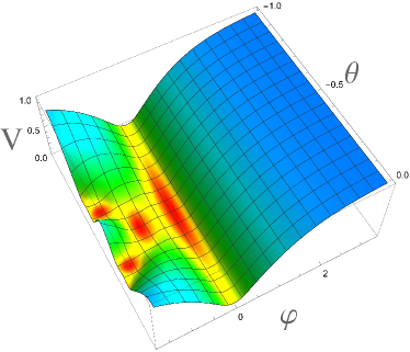
Figure 4: Potential (45) for $V_{0}=1$, $\tau_{2}=e^{\sqrt{2}\varphi}$ and $\tau_{1}=\theta$, $\alpha=1/3$, $n=1$. The potential is positive. The height of the potential is color-coded, from blue to red. The blue plateau approaches $V_{0}=1$ at large $\varphi\to+\infty$. Red corresponds to areas with $V\ll 1$ close to the minima of the potential.

In this limit, both potentials have a plateau behavior

$$V_{T}^{n}(\tau,\bar{\tau})|_{\tau_{2}\to\infty}=V_{0}\Big{(}{c\tau_{2}-1\over c\tau_{2}+1}\Big{)}^{n}\approx V_{0}(1-{4n\over c}{1\over\tau_{2}}+\cdots)$$ (52)

and

$$V_{E}^{n}(\tau,\bar{\tau})|_{\tau_{2}\to\infty}=V_{0}\Big{(}1-{1\over c\tau_{2}}\Big{)}^{n}\approx V_{0}(1-{2n\over c}{1\over\tau_{2}}+\cdots)$$ (53)

All properties of the potentials are confirmed in the plots below.

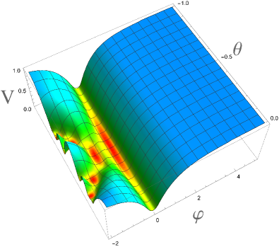
Figure 5: Potential (46) for $\tau_{2}=e^{\sqrt{2}\varphi}$ and $\tau_{1}=\theta$, $\alpha=1/3$, $n=1$.

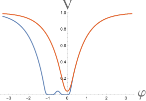
Figure 6: 2D slice of the otential (46) for $\tau_{2}=e^{\sqrt{2}\varphi}$ and $\tau_{1}=\theta=0$ (red curve), $\alpha=1/3$, and $\tau_{1}=\theta=-0.5$ (blue curve). The red curve coincides with the blue one at increasing values of $\varphi$. The unstable de Sitter saddle point can be seen here at $\tau=i$, i.e. at $\phi=0,\theta=0$, in the red curve at $V=4\times 10^{-2}$. The blue curve shows that at $\theta=-0.5,e^{{\sqrt{2}}\varphi}={\sqrt{3}\over 2}$ potential has a minimum.

By looking at these 3D and 2D potentials one can see that starting at some large positive $\phi$ at the plateau and some $\theta$ the cosmological evolution will proceed as follows. For a while, the axion $\theta$ remains close to its initial value whereas the inflaton moves towards smaller values of $\phi$. At $\tau=\theta+i,\phi=0$ the minimum is not reached yet. The evolution will continue near the exit in the direction of the minimum at $\tau=e^{2\pi i/3}$.

6.2 Examples with $\eta$-function

Consider the automorphic form $\hat{E}_{1}(\tau,\bar{\tau})$ defined in eq. (32) and normalize it at $|\tau|=1$. $I(\tau,\bar{\tau})$ here is proportional to $L_{\eta}$

$$I(\tau,\bar{\tau})\equiv{\hat{E}_{1}(\tau,\bar{\tau})\over E^{0}}\,,\qquad\hat{E}_{1}(\tau,\bar{\tau})|_{|\tau|=1}\equiv E^{0}\,,\qquad I(\tau,\bar{\tau})_{|\tau|=1}=1$$ (54)

At large $\tau_{2}$ and vanishing $\tau_{1}$ the properties of $\hat{E}_{1}(\tau,\bar{\tau})$ are given in eq. (36) so that

$$I(\tau,\bar{\tau})|_{\tau_{2}\to\infty,\tau_{1}=0}\to{\pi^{2}\over 3E^{0}}\tau_{2}\equiv c\tau_{2}$$ (55)

Our examples will depend on $SL(2,\mathbb{Z})$ invariant $I(\tau,\bar{\tau})$ in eq. (54).

The $SL(2,\mathbb{Z})$ invariant potentials are

$$V_{1}^{n}(\tau,\bar{\tau})=V_{0}\,\left({I(\tau,\bar{\tau})-1\over I(\tau,\bar{\tau})+1}\right)^{n}\,,\qquad V_{2}^{n}=V_{0}\left(1-I^{-1}(\tau,\bar{\tau})\right)^{n}$$ (56)

These potentials vanish at the point $|\tau|=1$ when $\tau=\pm{1\over 2}+i\sqrt{3/4}$. For $n>1$ we see that the potential has a minimum at $|\tau|=1$ when $\tau=\pm{1\over 2}+i\sqrt{3/4}$.

At large $\tau_{2}$ with the account of eq. (55)

$$V_{1}^{n}(\tau,\bar{\tau})|_{\tau_{2}\to\infty}\to V_{0}\left({c\tau_{2}-1\over c\tau_{2}+1}\right)^{n}$$ (57)

and

$$V_{2}(\tau,\bar{\tau})|_{\tau_{2}\to\infty}=V_{0}\Big{(}1-{1\over c\tau_{2}}\Big{)}^{n}$$ (58)

We recognize the attractor pattern studied before. The plots are very similar to the plots of the potentials with $j$-function, see e.g. Fig. 7 which shows the potential $V_{2}$ (56) for $n=1$.

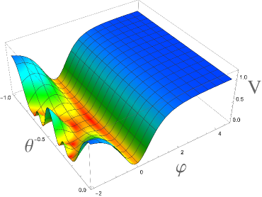
Figure 7: Potential $V_{2}$ (56) for $V_{0}=1$, $n=1$, $\alpha=1/3$, $\tau_{2}=e^{\sqrt{2}\varphi}$ and $\tau_{1}=\theta$.

6.3 Casas-Ibanez potential Casas:2024jbw and higher powers of it

The example already given in Casas:2024jbw depends on the ratio of two $SL(2,\mathbb{Z})$ invariants defined earlier:

$$V_{CI}=V_{0}{L_{G_{2}}(\tau,\bar{\tau})\over(2\pi L_{\eta}(\tau,\bar{\tau})+\tilde{N}_{0})^{2}}\ .$$ (59)

At ${\rm Im}(\tau)\to\infty$, assuming that the terms ${\log\tau_{2}\over\tau_{2}}$ in eq. (39) can be ignored during inflation,

$$V_{CI}\to V_{0}\Big{(}{\pi\over 3}-{1\over\tau_{2}}\Big{)}^{2}\ .$$ (60)

We have now confirmed that ignoring terms ${\log\tau_{2}\over\tau_{2}}$ during inflation is consistent, see eqs. (40), (41). The parameter $a$ in Casas:2024jbw is related to $\alpha$ in eq. (70) as

$$a^{2}={2\over 3\alpha}$$ (61)

The cosmological analysis in Casas:2024jbw of the model (59) was performed by arguing that one can ignore the effect of $\tau_{1}$ at large $\tau_{2}$. Therefore the computation of inflationary slow roll parameters was performed at $\tau_{1}=0$. We present the plot of such potentials in Fig. 8.

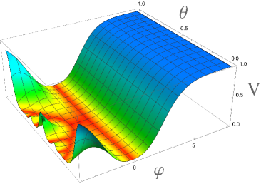
Figure 8: The figure presents the potential (59) for $\alpha=1$, $\tau_{2}=e^{\sqrt{2\over 3}\varphi}$, $\tilde{N}_{0}=25$ and $\tau_{1}=\theta$

Higher powers of the potential (59) such as

$$V_{CI}^{n}=V_{0}\Big{(}{L_{G_{2}}(\tau,\bar{\tau})\over(2\pi L_{\eta}(\tau,\bar{\tau})+\tilde{N}_{0})^{2})}\Big{)}^{n}\,,\qquad n>1$$ (62)

are also $SL(2,\mathbb{Z})$ invariant and inflationary predictions do not depend on $n$ for sufficiently small $\alpha$ and large $N_{e}$. In fact, the cosmological predictions of this model with $n=1$ were derived in Casas:2024jbw for various $a^{2}={2\over 3\alpha}$, not only for $a^{2}={2\over 3}$. They coincide with general $\alpha$-attractor predictions Kallosh:2013yoa ; Galante:2014ifa ; Kallosh:2021mnu given in (10).

7 General features of inflation in $SL(2,\mathbb{Z})$ invariant models

Plots of all $SL(2,\mathbb{Z})$ invariant potentials discussed in Section 6 show that at large $\varphi>0$ the axion $\theta=\tau_{1}$ forms a flat direction. As we already explained in Sec. 5, this is a general feature of such potentials that stems from the properties of the $j$- and $\eta$-functions. This fact significantly simplifies the investigation of inflation in such models.

An additional simplification follows from the properties of the hyperbolic geometry (2) Achucarro:2017ing ; Linde:2018hmx . It was found there that the axion field $\theta$ tends to freeze during inflation at large $\varphi$. To understand the origin of this effect, remember that the action of the scalar fields $\varphi$ and $\theta$ in hyperbolic geometry (2) is given by

$$\int d^{4}x\sqrt{-g}\left(-\frac{1}{2}\partial^{\mu}\varphi\partial_{\mu}\varphi-\frac{3\alpha}{4}e^{2\sqrt{\frac{2}{3\alpha}}\varphi}\partial_{\mu}\theta\partial^{\mu}\theta-V(\varphi,\theta)\right)\ .$$ (63)

The equations of motion for the homogeneous fields $\varphi$ and $\theta$ are

$$\ddot{\varphi}+3H\dot{\varphi}-\sqrt{\frac{3\alpha}{2}}e^{2\sqrt{\frac{2}{3\alpha}}\varphi}\,\dot{\theta}^{2}+V_{\varphi}=0\ ,$$ (64)

$$\ddot{\theta}+3H\dot{\theta}+2\sqrt{\frac{2}{3\alpha}}\dot{\varphi}\dot{\theta}+\frac{2}{3\alpha}e^{-2\sqrt{\frac{2}{3\alpha}}\varphi}V_{\theta}=0\ .$$ (65)

At $\varphi\gg\sqrt{\alpha}$ in the slow-roll approximation one has

$$3H\dot{\varphi}-\sqrt{\frac{3\alpha}{2}}e^{2\sqrt{\frac{2}{3\alpha}}\varphi}\dot{\theta}^{2}+V_{\varphi}=0\ ,$$ (66)

$$3H\dot{\theta}+\frac{2}{3\alpha}e^{-2\sqrt{\frac{2}{3\alpha}}\varphi}V_{\theta}=0\ .$$ (67)

Investigation of such potentials for $\alpha$-attractors shows that the value of $\dot{\theta}$ typically is suppressed by the factor of $e^{-\sqrt{2\over 3\alpha}\varphi}$ with respect to $\dot{\varphi}$. This is especially true for the models under consideration where the potentials are essentially flat in the $\theta$ direction. Moreover, investigation of such models performed in Achucarro:2017ing ; Linde:2018hmx have shown that perturbations of the field $\theta$ generated at early stages of inflation with $\varphi\gg\sqrt{\alpha}$ do not contribute to the resulting amplitude of adiabatic perturbations of metric. The conclusion was that there is a universality on multi-field attractors: general inflationary predictions of the new class of models coincide with general predictions of single-field $\alpha$-attractors for a large number of e-foldings $N$: $n_{s}=1-{2\over N}$, $r={12\alpha\over N^{2}}$. Thus, it is possible to have light fields on a hyperbolic manifold, which do not affect inflationary predictions since the light field $\theta$ practically does not move at the early stages of inflation.

Our preliminary investigation shows that this conclusion is also valid for the examples of the $SL(2,\mathbb{Z})$ invariant potentials presented above.

In application to the models studied in the previous section, this qualitative analysis suggests the following inflationary behavior. A long stage of inflation begins at large positive values of $\varphi$. As one can see from our general analysis and from Fig. 6, the behavior of the inflaton potential for all $\varphi\gg\sqrt{\alpha}$ does not depend on $\theta$ in the full range of initial values of $\theta$. Therefore the axion field practically does not change during inflation.

This means that if inflation begins at $\theta=0.5$, the field $\varphi$ rolls down to its global minimum with $\theta=0.5$ and a small negative value of $\varphi$, and inflation ends. However, for a full investigation of this regime, one may need a full numerical investigation. In particular, Fig. 6 shows that the potential has not one but two closely positioned Minkowski minima with $V=0$ at $\theta=0.5$. Thus inflation may end up in any of these two minima.

On the other hand, if inflation begins with $\theta=0$, the field $\varphi$ moves down to the shallow saddle point $\varphi=0,\theta=0$ where the potential has a tiny but positive value, and then the field eventually falls down to the same global minimum at $\tau=e^{2\pi i/3}$. A preliminary analysis of this second stage tells that this stage is very short and non-inflationary, and it does not affect inflationary predictions.

A qualitative analysis of the inflationary behavior of all models studied in Section 6 leads to very similar conclusions. However, the situation may change if one makes significant changes of the parameters. For example, we found that for some (fine-tuned) values of the parameters the height of the saddle point of the potential at $\varphi=\theta=0$ becomes very high, which may lead to a short secondary stage of inflation when the field $\theta$ rolls down to the minimum at $V=0$ at $\theta=0.5$. This regime resembles what happens in the two-field hybrid attractor models, where the combination of the two different inflationary regimes may lead to a copious production of primordial black holes, see e.g. Kallosh:2022vha ; Braglia:2022phb .

For completeness, we should say a few words on the properties of the potential at large negative values of $\varphi$, to make a more detailed comparison of the $SL(2,\mathbb{Z})$ attractors and the previously known classes of $\alpha$-attractors. As we discussed in Section 2, there are two qualitatively different classes of $\alpha$-attractors: E-model and T-models.

Potentials of the E-models have a plateau at large positive values of $\varphi$, and they blow up at large negative $\varphi$, see Fig. 1. At $\alpha=0$ these potentials coincide with the potential of the Starobinsky model. On the other hand, the potentials of the T-models depend on the absolute value of the field $\varphi$ and have two symmetric plateaus at large values of $\varphi$, see Fig. 2.

All $SL(2,\mathbb{Z})$ potentials are symmetric with respect to the change $\varphi\to-\varphi$ at $\tau_{1}\equiv\theta=0$. This is a direct consequence of the inversion symmetry at $\tau_{1}=0$. This means that they definitely do not belong to the class of E-models, and it would be very tempting to associate them with T-models. However, even though the $SL(2,\mathbb{Z})$ potentials at $\tau_{1}\equiv\theta=0$ are indeed very similar to the potentials of T-models shown in Fig. 2, the symmetry between the branches with positive and negative $\varphi$ is lost at $\theta\not=0$.

To explain it, in Fig. 9 we show the same potential (46) as in Fig. 4, but we show its part at large negative $\varphi$ and in a narrow interval of $\theta$ near $\theta=0$. This potential indeed has a plateau at large $|\varphi|$, $\theta=0$, but it is unstable for $\varphi<0$. This instability does not support inflation beginning at $\varphi<0$. That is why in our investigation we were analyzing inflation at $\varphi>0$.

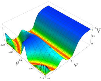
Figure 9: The figure presents the potential (59) for $\alpha=1$, $\tau_{2}=e^{\sqrt{2\over 3}\varphi}$, $\tilde{N}_{0}=25$ and $\tau_{1}=\theta$. This figure illustrates the behavior of the potential at large negative $\varphi$ in a narrow interval of $\theta$ near $\theta=0$.

8 Supersymmetric $SL(2,\mathbb{Z})$ models

In the framework of $\overline{D3}$ induced geometric inflation Kallosh:2017wnt ; McDonough:2016der supergravity is defined by a function $\mathcal{G}=K+\log|W|^{2}$ which includes in addition to our single superfield $T=-i\tau=e^{{\sqrt{2\over 3\alpha}}}-i\theta$ also a superfield $X$, which is nilpotent, i.e. $X^{2}=0$. It is a supergravity version of the uplifting $\overline{D3}$ brane which supports de Sitter vacuum in supergravityBergshoeff:2015tra ; Hasegawa:2015bza .

For a half-plane variable $T$, we consider the following Kähler invariant function $\mathcal{G}$

$$\mathcal{G}= -3\alpha\log(T+\bar{T})+G_{X\bar{X}}(T,\bar{T})X\bar{X}+\log|W_{0}+F_{X}\,X|^{2}$$ (68)

Here $X$ is a nilpotent superfield, $W_{0}$ is a constant defining the mass of gravitino, and $F_{X}$ is a constant, defining the auxiliary field vev. Following specific examples valid in $3\alpha=1$ case in Achucarro:2017ing and $\alpha<1$ case in Yamada:2018nsk ; Linde:2018hmx , in Kallosh:2022vha we proposed for the case $\alpha\leq 1$ the choice

$$G_{X\bar{X}}(T,\bar{T})=\frac{|F_{X}|^{2}}{(T+\bar{T})^{3\alpha}[\Lambda+V(T,\bar{T})]+3|W_{0}|^{2}(1-\alpha)}\,,\qquad\Lambda=F_{X}^{2}-3W_{0}^{2}$$ (69)

In this case, the bosonic action following from this supersymmetric construction is

$${{\cal L}(T,\bar{T})\over\sqrt{-g}}={R\over 2}-{3\alpha\over 4}\,{\partial T\partial\bar{T}\over({\rm Re}\,T)^{2}}-[\Lambda+V(T,\bar{T})]$$ (70)

If $\Lambda=|F_{X}|^{2}-3|W_{0}|^{2}>0$ and at the end of inflation $V(T,\bar{T})=0$ there is an exit into a de Sitter vacuum. The condition $\alpha\leq 1$ keeps the metric $G_{X\bar{X}}$ positive.

Now we take the bosonic model in eq. (44) and see that we have provided a supersymmetric version of it with the choice of the function $G_{X\bar{X}}$ defining the relevant $V(T,\bar{T})$. In this way, we have also embedded the bosonic theory into a version of supergravity with de Sitter exit of inflation. This gives us a supersymmetric generalization of the bosonic theories we constructed and studied in this paper and applied to cosmology.

9 Summary

Supergravity theories have various duality symmetries with continuous parameters, for example, $SL(2,\mathbb{R})$ symmetry. It is believed that non-perturbative quantum effects break these continuous symmetries to their discrete subgroups, $SL(2,\mathbb{Z})$ in our example. Therefore there was a strong interest to modular inflation over the years. Significant progress was achieved in Casas:2024jbw when the idea of $SL(2,\mathbb{Z})$ symmetry was first time implemented in a plateau potential with a particular choice of automorphic forms.

The $SL(2,\mathbb{Z})$ symmetric potentials as a function of the complex field $\tau=\theta+ie^{\sqrt{2\over 3\alpha}\varphi}$ have the following symmetry under inversion and translation

$$V(\tau,\bar{\tau})=V\Big{(}-{1\over\tau},-{1\over\bar{\tau}}\Big{)}\,,\qquad V(\tau,\bar{\tau})=V(\tau+1,\bar{\tau}+1)\ .$$ (71)

There are special self-dual points of the inversion symmetry when

$$|\tau|=1={1\over|\tau|}:\qquad\tau=i,\qquad\tau=e^{2\pi i\over 3}$$ (72)

In this work, we have found that there are many different $SL(2,\mathbb{Z})$ symmetric plateau potentials with various choices of automorphic forms. We have observed that in modular potentials a de Sitter saddle point at $\tau=i$ and a Minkowski minimum at $\tau=e^{2\pi i/3}$ are generic. This feature is particularly easy to see analytically in the example of a potential depending on a modular $j$-function, see Sec. 6.1. All 3D plots show this feature as well as the plateau at $\phi\to\infty$ with a flat axion direction as predicted by the properties of the modular functions. For example, properties of a logarithm of a Dedekind function derived in Atiyah1987 , see eq. (36) and properties of a logarithm of a shifted $|j|^{2}$-function as given in eqs. (30), (31), help to understand why these potentials have a plateau.

As long as they have an exponential approach to the plateau, as in earlier $\alpha$-attractor models Kallosh:2013yoa ; Galante:2014ifa ; Kallosh:2015zsa ; Carrasco:2015uma ; Carrasco:2015rva ; Carrasco:2015pla , i.e.

$$V\to V_{0}(1-e^{-\sqrt{2\over 3\alpha}\varphi}+\dots)$$ (73)

they give universal predictions for inflationary observables, depending only on $V_{0}$ and $\alpha$ shown in eq. (10).

The issue of the flat axion direction at the plateau, present in modular models here, was studied in the earlier $\alpha$-attractor models Achucarro:2017ing ; Linde:2018hmx . We have used this analysis here, based on hyperbolic geometry. We have described the general features of inflation in $SL(2,\mathbb{Z})$ invariant models in Sec. 7 and presented its supersymmetric version in Sec. 8.

References

- (1) G.F. Casas and L.E. Ibáñez, Modular Invariant Starobinsky Inflation and the Species Scale, 2407.12081.
- (2) R. Kallosh, A. Linde and D. Roest, Superconformal Inflationary -Attractors, JHEP 11 (2013) 198 [1311.0472].
- (3) M. Galante, R. Kallosh, A. Linde and D. Roest, Unity of Cosmological Inflation Attractors, Phys. Rev. Lett. 114 (2015) 141302 [1412.3797].
- (4) R. Kallosh and A. Linde, Escher in the Sky, Comptes Rendus Physique 16 (2015) 914 [1503.06785].
- (5) J.J.M. Carrasco, R. Kallosh, A. Linde and D. Roest, Hyperbolic geometry of cosmological attractors, Phys. Rev. D92 (2015) 041301 [1504.05557].
- (6) J.J.M. Carrasco, R. Kallosh and A. Linde, Cosmological Attractors and Initial Conditions for Inflation, Phys. Rev. D92 (2015) 063519 [1506.00936].
- (7) J.J.M. Carrasco, R. Kallosh and A. Linde, -Attractors: Planck, LHC and Dark Energy, JHEP 10 (2015) 147 [1506.01708].
- (8) A. Achúcarro, R. Kallosh, A. Linde, D.-G. Wang and Y. Welling, Universality of multi-field -attractors, JCAP 1804 (2018) 028 [1711.09478].
- (9) A. Achúcarro, A. Linde, D.-G. Wang, Y. Welling and Y. Yamada, Hypernatural inflation, JCAP 1807 (2018) 035 [1803.09911].
- (10) R. Kallosh, A. Linde, D. Roest and Y. Yamada, induced geometric inflation, JHEP 07 (2017) 057 [1705.09247].
- (11) E. McDonough and M. Scalisi, Inflation from Nilpotent Kähler Corrections, JCAP 1611 (2016) 028 [1609.00364].
- (12) F. Farakos, A. Kehagias and A. Riotto, Liberated = 1 supergravity, JHEP 06 (2018) 011 [1805.01877].
- (13) LiteBIRD collaboration, Probing Cosmic Inflation with the LiteBIRD Cosmic Microwave Background Polarization Survey, PTEP 2023 (2023) 042F01 [2202.02773].
- (14) S. Ferrara and R. Kallosh, Seven-disk manifold, -attractors, and modes, Phys. Rev. D94 (2016) 126015 [1610.04163].
- (15) R. Kallosh, A. Linde, T. Wrase and Y. Yamada, IIB String Theory and Sequestered Inflation, 2108.08492.
- (16) R. Kallosh and A. Linde, BICEP/Keck and cosmological attractors, JCAP 12 (2021) 008 [2110.10902].
- (17) R. Kallosh and A. Linde, Universality Class in Conformal Inflation, JCAP 1307 (2013) 002 [1306.5220].
- (18) BICEP/Keck collaboration, Improved Constraints on Primordial Gravitational Waves using Planck, WMAP, and BICEP/Keck Observations through the 2018 Observing Season, Phys. Rev. Lett. 127 (2021) 151301 [2110.00483].
- (19) B.J. Broy, M. Galante, D. Roest and A. Westphal, Pole inflation — Shift symmetry and universal corrections, JHEP 12 (2015) 149 [1507.02277].
- (20) M. Atiyah, The logarithm of the dedekind n-function., Mathematische Annalen 278 (1987) 335.
- (21) L.J. Dixon, V. Kaplunovsky and J. Louis, Moduli dependence of string loop corrections to gauge coupling constants, Nucl. Phys. B 355 (1991) 649.
- (22) M.B. Green, J.G. Russo and P. Vanhove, Automorphic properties of low energy string amplitudes in various dimensions, Phys. Rev. D 81 (2010) 086008 [1001.2535].
- (23) R. Kallosh and A. Linde, Dilaton-axion inflation with PBHs and GWs, JCAP 08 (2022) 037 [2203.10437].
- (24) M. Braglia, A. Linde, R. Kallosh and F. Finelli, Hybrid -attractors, primordial black holes and gravitational wave backgrounds, JCAP 04 (2023) 033 [2211.14262].
- (25) E.A. Bergshoeff, D.Z. Freedman, R. Kallosh and A. Van Proeyen, Pure de Sitter Supergravity, Phys. Rev. D92 (2015) 085040 [1507.08264].
- (26) F. Hasegawa and Y. Yamada, Component action of nilpotent multiplet coupled to matter in 4 dimensional supergravity, JHEP 10 (2015) 106 [1507.08619].
- (27) Y. Yamada, U(1) symmetric -attractors, JHEP 04 (2018) 006 [1802.04848].