A hybrid SIAC – data-driven post-processing filter for discontinuities in solutions to numerical PDEs

Abstract

We introduce a hybrid filter that incorporates a mathematically accurate moment-based filter with a data driven filter for discontinuous Galerkin approximations to PDE solutions that contain discontinuities. Numerical solutions of PDEs suffer from an $\mathcal{O}(1)$ error in the neighborhood about discontinuities, especially for shock waves that arise in inviscid compressible flow problems. While post-processing filters, such as the Smoothness-Increasing Accuracy-Conserving (SIAC) filter, can improve the order of error in smooth regions, the $\mathcal{O}(1)$ error in the vicinity of a discontinuity remains. To alleviate this, we combine the SIAC filter with a data-driven filter based on Convolutional Neural Networks. The data-driven filter is specifically focused on improving the errors in discontinuous regions and therefore only includes top-hat functions in the training dataset. For both filters, a consistency constraint is enforced, while the SIAC filter additionally satisfies $r-$moments. This hybrid filter approach allows for maintaining the accuracy guaranteed by the theory in smooth regions while the hybrid SIAC-data-driven approach reduces the $\ell_{2}$ and $\ell_{\infty}$ errors about discontinuities. Thus, overall the global errors are reduced. We examine the performance of the hybrid filter about discontinuities for the one-dimensional Euler equations for the Lax, Sod, and sine-entropy (Shu-Osher) shock-tube problems.

1 Introduction

In this article, we develop a hybrid filter that allows for filtering both smooth and discontinuous regions. This is motivated by the need to approximate solutions to nonlinear systems such as the Euler equations. Computing solutions to inviscid flow problems such as the Euler equations is challenging due to shock waves that arise. Techniques to solve this system fall into two categories: shock-fitting and shock-capturing. While the shock-fitting method relies on the Rankine-Hugoniot conditions to introduce the shock into the solution, the shock-capturing method solves the Euler equations in conservative form and computes the shocks or discontinuities as part of the solution [25, 45] and are the focus herein. Shock-capturing methods suffer from spurious oscillations due to Gibbs phenomenon in the presence of shocks. As a consequence, shock-capturing solutions are accurate in smooth regions or near weak shocks but suffer from the unphysical oscillations and instabilities due to strong shocks. This yields an $\mathcal{O}(1)$ error in the neighborhood of a discontinuity that pollutes the quality of the solution throughout the domain [17]. The $\mathcal{O}(1)$ error in the neighborhood of a discontinuity for numerical solutions to PDEs can be avoided when the discontinuity is placed at an element interface in a discontinuous Galerkin (DG) approximation. Traditionally, filters can be applied to the solution to reduce the errors in smooth regions, which in this work is done via Smoothness-Increasing Accuracy-Conserving (SIAC) filtering. Here, the focus is on filtering for discontinuous regions. This is done via a data-driven filter that allows for reducing the error in the discontinuous region.

The mechanisms to recover accuracy away from discontinuities, such as filters, post-process the numerical solution in order to recover accuracy away from discontinuites and reduce spurious oscillations near the discontinuity. They can also extract more resolution for enhanced accuracy. This is especially necessary when numerical data suffers from aliasing error, reduced pointwise error due to discretization, Gibbs phenomenon, or other artefacts [9, 16, 17, 34, 41, 47]. Filters aim to recover uniform convergence in the approximation, but improvement results are limited to smooth regions. If discontinuities arise in a $\mathcal{C}^{\infty}$ smooth solution to a PDE, the piecewise $\mathcal{C}^{\infty}$ solution cannot be recovered with that same order because of errors due to discontinuities polluting the approximation globally. Mock and Lax [32] showed that by post-processing the numerical approximation, the exact solution and its derivatives can be recovered with an order $\nu-\delta$, where $\delta$ depends on the number of vanishing moments of the post-processing kernel filter. This relies however on suitable pre-processing of data. Post-processing kernels have since achieved up to an order $2\nu-1$ for the SIAC kernel [41] or a user-specified order for the exponential kernel, which technically does not satisfy the definition of a filter given in [47]. These enhanced orders of accuracy are restricted to smooth regions only, with the error in the neighborhood about a discontinuity remaining at order one [17]. The numerical solution in the region about a shock or contact discontinuity can only converge to the average of the left and right limits of the discontinuity [17, 32].

Convolutional filters using convolutional neural networks (CNNs) have enabled a data-driven approach to post-processing and filtering numerical data. CNNs have been widely used for the fields of visual tracking and recognition [6, 13, 46]. In addition, CNNs have been combined with other filtering and NN techniques to extract spatial and temporal frequency information from data with different frequencies [18]. While CNNs have been used to learn time-dependent PDEs from limited data [37], the post-processing of numerical PDE solutions using CNNs has not yet been considered.

Other machine learning approaches to solve PDEs to resolve challenges from traditional PDE solving methods have been implemented, such as the physics-informed neural network (PINN) as introduced by Raissi et al. [38], which can solve both the forward and inverse problems of PDEs and has been used to solve the Euler equations. Mao et al. [28] solved the Euler equations using PINNs and demonstrated that PINNs are not as accurate as traditional numerical methods in the forward problem but are more superior for the inverse problems. Specifically, smooth problems were well approximated but problems with discontinuities were more sensitive to the position of the learning point in the domain, with better accuracy when learning points were more clustered near the discontinuities. Splitting the training between continuous and discontinuous sub-domains has been done in [19]. In addition, Liu et al. calculate discontinuities more accurately by deviating the training to smooth regions only by using a weighted equation method that recognizes discontinuities are not captured by the strong form of the PDEs nor do NNs have theoretical guarantees to approximate first-order discontinuities [27]. More recently, in Liang et al.’s study [26] of continuous and discontinuous compressible flows in a converging-diverging channel demonstrated that default settings of PINNs failed to resolve discontinuities even with more training points and epochs, or would yield trivial solutions. Instead, they relied on adapting the weights on the momentum loss and fixing the Dirichlet boundary conditions as hard constraints.

Consequentially, improving errors about discontinuities in the solutions of Euler equations where shock waves arise remains an active area of research and has been the motivation when developing a filter for discontinuities. Given that post-processing filters alone, or PINNs as a direct numerical simulation tool, can still be further improved, the focus is combining machine learning with the SIAC filter to create a hybrid SIAC – data-driven filter to reduce error about discontinuities. Data-driven techniques may provide enhancements to analytical methods where they fall short. For example, the physics-informed neural network (PINN) [38] is more superior than traditional numerical methods when solving the inverse Euler problem, but when used for the forward Euler problem, PINNs still have issues tracking the discontinuities accurately [28, 19, 27, 26]. While a neural network (NN)-based troubled cell detector [39, 40, 51] has been introduced as a machine learning tool for numerical PDEs, other efforts to leverage the power of data and computation to learn patterns within numerical PDE solutions have not yet been explored. To our knowledge, combining learned convolutional filters with traditional filters for post-processing numerical PDE solutions to improve the approximation about a discontinuity has not yet been investigated.

This work establishes a novel hybrid, data-driven SIAC filter, where the SIAC filter is initially applied globally followed by an adapted SIAC–data-driven filter with Hermite interpolation in the regions about discontinuities. We contribute a data-driven filter that is based on an output-constrained CNN whose outputs satisfy the kernel consistency constraint, which ensures the data-driven filters can reproduce constant data [41]. The SIAC filter achieves superconvergence by reducing errors and increasing convergence rates in the smooth regions [9, 41], while the combination of the adapted SIAC filter, data-driven filter, and Hermite polynomial interpolation reduces the $\mathcal{O}(1)$ error about the discontinuities. In order to construct an effective discontinuity-targeted hybrid filter, we establish 1) a training dataset that captures the discontinuities that arise in the Euler problem, 2) consistency as a hard constraint, and 3) a discontinuity window detection approach that captures the neighborhood about a discontinuity. These are extensive challenges in developing this novel hybrid data-driven SIAC filter that reduces the error at discontinuities and thus the initial scope of this work is limited to one-dimensional data.

The remainder of this paper is organized as follows. Following the relevant background presented in Section 2, we present the development of a hybrid data-driven filter (Section 3) and the setup for numerical experiments (Section 4). Finally, the article concludes with the results (Section 5) and a discussion (Section 6).

2 Background

2.1 Filters

An overview on the theory of filters is presented below in Section 2.1.1 in the context of spectral filters. This is then followed by a discussion of the SIAC kernel in Section 2.1.2.

2.1.1 Spectral Filters

To illustrate how filters work in the context of a spectral approximation, a truncated Fourier series representation is considered for the approximation to the solution to a PDE, $u\in\Omega\subset{\mathbb{R}}$. The truncated Fourier series sum with $M$ Fourier modes $\mathcal{P}_{M}u$ is defined as

$$\mathcal{P}_{M}u=\sum_{m=-M/2}^{M/2}\hat{u}_{m}e^{i\frac{2\pi m}{|\Omega|}x},$$ (1)

and the Fourier modes or coefficients are computed as

$$\hat{u}_{m}=\frac{1}{|\Omega|}\int_{\Omega}u(x)e^{-i\frac{2\pi m}{|\Omega|}\pi x}.$$ (2)

Now, consider an approximation with a discontinuity. The error at the discontinuity will remain large, and even if the resolution is increased, the error at the discontinuity is not improved. The error between the exact solution $u$ and the approximation $\mathcal{P}_{M}u$ is up to order $1/\sqrt{M}$. While the function may be smooth away from the discontinuity and periodic, the global rate of convergence is governed by the presence of the discontinuity due to the global expansion basis. The approximation converges in the mean, but it is not uniformly convergent due to the presence of the discontinuity. The slow convergence away from a discontinuity and the non-uniform convergence near the discontinuity constitute the behavior in Gibbs phenomenon [17]. Gibbs oscillations pollute the numerical approximation over the entire domain. Filtering is then utilized to recover spectral accuracy away from the discontinuity [47].

The Gibbs behavior is exhibited in the slow decay of the expansion coefficients. Filtering aims to modify the expansion coefficients so that they have a faster rate of decay. A well-designed filter will accelerate the convergence away from a discontinuity and will not alter the non-uniform convergence near a shock [17]. As defined in [47], a filter of order $q$ is a real and even function, $\sigma(\eta)\in\mathcal{C}^{q-1}(-\infty,\infty)$, with the following properties:

$$\sigma(\eta) =0,\quad|\eta|\geq 1$$ (3a)

$$\sigma(0) =1,$$ (3b)

$$\sigma^{(i)}(0)=\sigma^{(i)}(1) =0,\quad i=1,2,\ldots,q-1.$$ (3c)

A truncated continuous polynomial approximation can be filtered by altering the continuous expansion coefficients $\hat{u}_{m}$ by $\sigma(|m|/(M/2))$. The filtered approximation is then defined as

$$\mathcal{P}_{M}^{\sigma}u(x)=u_{M}^{\sigma}(x)=\sum_{m=-M/2}^{M/2}\sigma\left(\frac{|m|}{M/2}\right)\hat{u}_{m}e^{-i\frac{2\pi m}{|\Omega|}x}.$$ (4)

Note that this is equivalent to convolutional filtering for a non-Fourier series representation. By definition, a filter will not modify the mean of the solution, but will dampen the higher modes as $\sigma\left(\frac{|m|}{M/2}\right)\rightarrow 0$ smoothly when $|m|\rightarrow\frac{M}{2}$. If the high modes were to be removed abruptly, the convergence rate in smooth regions will not be improved. Properties (3b-3c) are proven in [47] to be the necessary conditions for $|u(x)-u_{M}^{\sigma}(x)|=\mathcal{O}(M^{1/2-q})$, when $u$ has at least one discontinuity.

Designing effective filters continues to be a challenge. Some traditional filters include the Cesáro, raised cosine, Lanczos, and exponential filters. While the Cesáro kernel is of order 1 and does not regain accuracy in smooth regions, both the raised cosine and Lanczos filters are second order and reduce error away from the discontinuity, with slightly less improvement for the Lanczos filter. The exponential filter, although not satisfying property 3c, allows for adjustable order and is popular for nonlinear PDEs, where the growing Gibbs oscillations may lead to scheme instability [17]. However, the exponential filter can be overly dissipative.

2.1.2 The SIAC Kernel

The SIAC filter was developed as a post-processing tool to extract accuracy and increase smoothness in DG methods for hyperbolic equations [41, 5]. This filter is based on the earlier work done by Bramble and Schatz [1] and Cockburn et al. [3]. The SIAC filter achieves superconvergence by reducing errors and increasing convergence rates given polynomial reproduction in the SIAC kernel construction. A DG numerical approximation of order $p+1$ can achieve up to $2p+1\ (2\nu-1=2p+1)$ order of accuracy in the $L^{2}$ norm after SIAC post-processing for linear hyperbolic equations [41, 9]. The SIAC filter has been adapted for nonuniform meshes [5], multi-dimensional problems using tensor products [5], line filtering [8, 9], and hexagonal splines [31], as well as enhanced multiresolution analysis [34].

The SIAC kernel is constructed as a weighted average of central B-splines,

$$K^{(r+1,k+1)}(\bar{x})=\sum_{\gamma=0}^{r}c_{\gamma,\bar{x}}B^{(k+1)}(\bar{x}-x_{\gamma}),$$ (5)

where $\bar{x}$ is the evaluation point (kernel center) and $B^{(k+1)}(\bar{x}-x_{\gamma})$ is a B-spline of order $k+1$ centered at the point $x_{\gamma}$, and $r$ is the number of moments the kernel satisfies. For the symmetric kernel, $x_{\gamma}=-\frac{r}{2}+\gamma$, the coefficients $c_{\gamma,\bar{x}}$ are solved to satisfy consistency, $\int_{\mathbb{R}}K(x)dx=1$, and polynomial reproduction of the kernel, namely, $K\ast x^{p}=x^{p}$ or $\int_{\mathbb{R}}K(x-y)y^{p}dy=x^{p}$ for $p=0,\ldots,r$ [41, 9]. Polynomial reproduction is equivalent to satisfying moments. In the case where the kernel is symmetric, the coefficients do not rely on the evaluation point.

The SIAC filtered approximation is applied as a convolution in physical space. Although this may vary from the presentation on the spectral filters in Section 2.1.1, they are equivalent in Fourier space. The SIAC filtered approximation is defined as follows,

$$u_{h}^{*}(x,T) =(K_{H}\ast u_{h})(x,t)=\int_{\mathbb{R}}K_{H}^{(r+1,k+1)}(x-\xi)u_{h}(\xi,t)d\xi,$$ (6a)

$$=\frac{1}{H}\int_{\mathbb{R}}K^{(r+1,k+1)}\left(\frac{x-\xi}{H}\right)u_{h}(\xi,t)d\xi,$$ (6b)

where $H$ is the SIAC kernel scaling that ensures the filtered solution is only utilizing the nearest neighbors. The kernel scaling $H$ is taken to be the element size $h$ for uniform meshes [9] but other $H$ values have been studied [7]. Generally, a SIAC kernel of $2p+1$ B-splines of order $p+1$ is considered for a sample that is approximated using a DG degree $p$. Henceforth, we will synonymously use the terms “filter” and “kernel”.

2.2 Euler equations

This work examines the performance of the hybrid filter on numerical solutions to the Euler equations, which are known for the shock waves that arise. For the Euler equations for compressible gas dynamics, the three equations include the conservation of mass, momentum, and energy. In conservative form, the Euler equations are presented as

$$\boldsymbol{u}_{t}+\boldsymbol{f}(\boldsymbol{u})_{x}=0$$ (7)

with $\boldsymbol{u}=(\rho,\rho u,E)^{T}$ and $\boldsymbol{f}(\boldsymbol{u})=\left(\rho u,\rho u^{2}+p,(E+p)u\right)^{T}$, where the conservative variables are density $\rho$, momentum $\rho u$, and energy $E$, while the primitive variables are density $\rho$, velocity $u$, and pressure $p$. The total energy $E$ constitutes the kinetic and internal energy, or $E=\frac{1}{2}\rho u^{2}+\rho e$, with $e$ being the specific internal energy or the internal energy per unit mass [25]. We can replace the internal energy by the term $p/(\gamma-1)$ to result in the equation of state

$$E=\frac{p}{\gamma-1}+\frac{1}{2}\rho u^{2},$$ (8)

where, in this context, $\gamma$ is the ratio of specific heats at constant pressure and volume, $c_{p}/c_{v}$. For an ideal gas, which will be considered here, we know that $\gamma=1.4$. The conservative form of the Euler equations (Eq. 7) is solved numerically using the modal discontinuous Galerkin (DG) method [2, 4].

We can also re-write the equations Eq. 7 in terms of the primitive variables, as follows,

$$\boldsymbol{q}_{t}+A(\boldsymbol{q})\boldsymbol{q}_{x}=0,$$ (9)

where

$$A(\boldsymbol{q})=\left(\begin{matrix}u&\rho&0\\ 0&u&1/\rho\\ 0&\gamma p&u\end{matrix}\right).$$

Eigenvalue decomposition can be used to solve the system, which provides the same eigenvalues as those of the flux Jacobian in Eq. 7, i.e. $\lambda=\{u-c,u,u+c\}$, where $c=\sqrt{\frac{\gamma p}{\rho}}$ is the speed of sound in the medium. These eigenvalues are real and thus the Euler system is hyperbolic. As $A=A(\boldsymbol{q})$, the system is quasilinear and thus Eq. 9 is also called the quasilinear form of the Euler equations [21].

While “shock” is often interpreted as any type of discontinuity, we clarify the distinction between the different discontinuities in these invsicid compressible flow problems, as derived by Jeffrey [20]. The contact discontinuity occurs when the jump about the density profile is non-zero, whereas those of the pressure and the fluid velocity vectors are zero. On the other hand, a shock discontinuity results in discontinuities about the density, velocity, and pressure profiles. Additionally, the rarefaction wave is another discontinuity type. We focus herein on the contact and shock discontinuities that produce the $\mathcal{C}^{0}$ discontinuity conducive to the $\mathcal{O}(1)$ error profile that is most challenging to tackle in post-processing methods.

2.3 Initial Conditions

In the numerical experiments, we consider the following standard test problems for the one-dimensional Euler system: Sod [44], Lax [24], and Shu-Osher [43]. These test problems represent different initial conditions of the ideal, compressible gas in a one-dimensional shock tube.

The Sod shock tube initial condition for the one-dimensional Euler system of equations is defined on $\Omega=[-5,5]$ with the following two-state initial condition,

$$(\rho_{0},u_{0},p_{0})=\begin{cases}(1,0,1),&x<0,\\ (0.125,0,0.1),&x\geq 0,\end{cases}$$ (10)

with Dirichlet boundary conditions. This test case is evolved until final time $T_{f}=2$ at which point it develops a rarefaction wave and contact and shock discontinuities in the density profile.

A similar shock tube initial condition is the Lax problem, which includes the same domain and boundary conditions, but the two states at initial time are defined as

$$(\rho_{0},u_{0},p_{0})=\begin{cases}(0.445,0.698,3.528),&x<0,\\ (0.5,0,0.571),&x\geq 0.\end{cases}$$ (11)

This problem is time-evolved to final time $T_{f}=1.3$, which also develops the same discontinuities as in the Sod problem. However, the contact and shock discontinuities are much sharper and thus more susceptible to error and spurious oscillations.

Finally, the sine-entropy or Shu-Osher problem [43] presents non-constant states in $\Omega=[-5,5]$ and is given as

$$(\rho_{0},u_{0},p_{0})=\begin{cases}(3.857143,2.629369,10.33333),&x<-4,\\ (1+0.2\sin(5x),0,1)&x\geq-4,\end{cases}$$ (12)

with Dirichlet boundary conditions enforced. The problem is evolved to $T_{f}=1.8$ and demonstrates both weak and strong shocks about the sinusoidal density profile.

The exact reference solutions for the primitive variables for the Lax, Sod, and sine-entropy problems are shown in Fig. 1, where the Clawpack solver as used in [21] is used to solve the Riemann Lax and Sod exact solutions, while the exact reference for the sine-entropy problem is computed with $N=30,000$ elements and degree $p=0$. Both the Sod and Lax plots include rarefaction, contact, and shock discontinuities, as appearing in the domain from left to right. Whereas the rarefaction discontinuity has a $\mathcal{C}^{1}$ discontinuity, the contact and shock discontinuities are the $\mathcal{C}^{0}$ discontinuities that are the primary focus of this work. The sine-entropy problem includes a strong sinusoidal shock near $x=2.4$ and weaker shocks, but only the strong shock is examined herein.

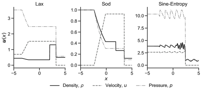
Figure 1: The Euler exact reference solutions for the Lax, Sod, and sine-entropy (Shu-Osher) test problems at their respective benchmark final times, $T_{f}=\{1.3,2,1.8\}$. Note the different data ranges for each of the problems.

3 A Hybrid SIAC – Data-Driven Filter

The main contribution of this work is the development of a hybrid data-driven filter. This requires balancing a filter that minimizes the pollution arising from the discontinuity in smooth regions with the challenge of improving the errors near a discontinuity through a data-driven technique. In order to fuse these filters, we additionally utilize interpolation techniques. After first presenting the data-driven filter (Section 3.1), the construction of the hybrid filter is presented in Section 3.2 followed by the setup for the discontinuity windows (Section 3.3).

Algorithm 1 CNN Forward Step

1:function forward($u_{h}^{\ast}$):

2:     compute NN-filtered data: $u_{h}^{\ast_{NN}}=K_{\Theta}\ast u_{h}^{\ast}$

3:     compute normalizing constant: $c_{\Theta}=\frac{1}{N}\sum K_{\Theta}\ast\mathbf{1}^{N}$

4:     return output: $u_{h}^{\ast_{NN}}/{c_{\Theta}}$

5:end function

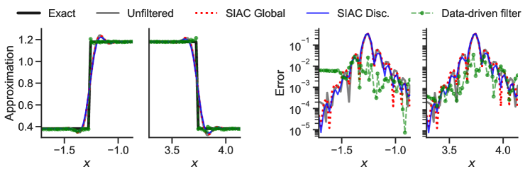
Figure 2: SIAC filtering and data-driven filtering with a global SIAC filter with full kernel support and order-2 B-splines (red dotted), an adapted SIAC filter for the discontinuities with a single order-1 B-spline (blue), and the data-driven filter (green dashed). The left two plots show the approximations of a contact and shock discontinuity of a training sample of DG degree 3, while the right two plots include their respective pointwise error.

3.1 The data-driven filter

Our data-driven filter is comprised of a residual CNN that satisfies a kernel consistency constraint. In particular, we train a kernel $K_{\Theta}$ through the following constrained optimization problem,

$$\min_{\Theta}\frac{1}{M}\sum_{j=1}^{M}\|K_{\Theta}*(K_{H}\ast u_{j,h})-u_{j}\|_{2}^{2}\quad\text{subject to}\quad\int_{\mathbb{R}}K_{\Theta}(x)dx=1,$$ (13)

where $u_{j}\in\mathcal{U}$ is the exact solution for sample $j$; $\mathcal{U}$ is the class of functions that includes solutions to $u_{t}=\mathcal{N}(u)$, where $\mathcal{N}$ is a nonlinear differential operator whose solution develops $\mathcal{C}^{0}$ discontinuities in time (although other types of discontinuities and differential operators may be considered); $u_{j,h}$ is the numerical approximation to $u_{j}$ for a given discretization $h$; $K_{H}$ is the SIAC kernel as defined in Section 2.1.2 with a kernel scaling of $H$; and $M$ is the total number of samples in the training dataset. The input data to the CNN, $K_{H}\ast u_{j,h}$, and its true output, $u_{j}$, are defined at a window about a discontinuity. Given the lack of continuity in those regions and failure to reproduce higher-order moments, we consider an adapted SIAC kernel $K_{H}$ for discontinuity data that preserves consistency alone. Here, the objective function is a sample average approximation of the expectation of the random variable consisting of DG solutions to hyperbolic PDEs about discontinuities, and the constraint enforces consistency, which is necessary in order to preserve the information of the underlying data [41, 9].

The constraints are enforced by computing the normalizing constant

$$c_{\Theta}=\int_{\mathbb{R}}K_{\Theta}(x)dx.$$ (14)

We leverage automatic differentiation in PyTorch [22] to backpropagate through the normalized output. While deep learning architectures such as implicit networks [11, 29, 30, 15] are able to provide hard constraints on their outputs, the proposed constraint is simple to implement in a way that does not require making the network implicit. The pseudocode, presented in Algorithm 1, indicates how the normalizing constant $c_{\Theta}$ in Eq. 14 is computed in the network forward step.

3.2 Constructing the Hybrid Filter Solution

Importantly, we emphasize that using only the SIAC-filtered approximation does not reduce the errors about the discontinuities. As an example with a degree-3 DG approximation in Fig. 2, we show the data post-processed with two SIAC filters. The “SIAC Global” filter includes a full kernel support and order-2 B-splines, while “SIAC Disc.” is a consistency-only SIAC filter for the discontinuity region including one single order-1 B-spline, or a moving average kernel. For both SIAC-filtered approximations, even when the kernel support and order of the B-spline shrink, the error at the two discontinuities maintain the underlying $\mathcal{O}(1)$ error band of the unfiltered DG data, although the consistency-only SIAC filter yields lower error values slightly farther from the discontinuity location. The training process for the data-driven filter leverages such large errors and as a consequence, trains for the parameters $\Theta$ such that the errors are reduced about the discontinuity window, with the largest error at the point of discontinuity. This is shown in the data-driven filtered approximation in Fig. 2, which shows a reduction of the $\mathcal{O}(1)$ error at the contact and shock discontinuities for this sample drawn from the training data distribution. The data-driven filter maintains the low error within the neighborhood of the discontinuity, but the error hits a floor for data with an underlying error of less than $10^{-3}$.

We can construct our hybridized filter to build on the SIAC filter at the discontinuity. The hybridized filter merges the consistency-only SIAC filter, which is applied to the discontinuity window, with the data-driven filter applied to the SIAC data at the cell where the discontinuity is located. The data-driven filter reduces the error for both the unfiltered and SIAC-filtered approximations for the degree-3 training sample shown in Fig. 2, but its performance may vary depending on the DG degree and sample distribution. As such, we apply the data-driven filter to the cell with the discontinuity location, where the error is largest. To fuse the two filtering methods, Hermite polynomial interpolation is applied to the cells adjacent to the discontinuity cell. The SIAC filter uses $K_{H}$ as defined in Section 2.1.2 with kernel scaling $H=h$ and one single order-1 B-spline, or a moving average filter. This choice of SIAC filter reduces the over-smoothing that may arise for SIAC kernels with higher-order B-splines that are more advantageous to use in smoother regions in order to extract superconvergence properties [9]. A SIAC filter that preserves consistency alone is in fact accuracy-conserving for discontinuity data, and thus at most constant data can be reproduced to the left and right of the discontinuity. With such an adapted SIAC filter, the polluted error about the discontinuity is less spread across neighboring cells given a more localized kernel support due to the single B-spline. The data-driven filter uses the learned residual convolutional network $K_{\Theta}$, and it is applied to the element with the discontinuity. To maintain smoothness about such data-driven filtered data and the underlying SIAC data about the discontinuity, Hermite polynomial interpolation with degree $\min(2,p)$ is applied to the adjacent cells to the discontinuity in order to preserve pointwise data evaluation and their derivatives [10]. This varies from the Hermite WENO (HWENO) method [35], which uses a Hermite polynomial fit about a 3-cell stencil to limit troubled cell data in Runge-Kutta DG (RKDG) schemes. Here, Hermite interpolation is only used to update adjacent cells to the discontinuity while leveraging the data-driven filter for sub-cell feature extraction of the discontinuity location, which is not achieved in the HWENO results to the Lax problem in [35].

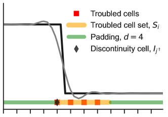
Figure 3: Demonstration of the discontinuity window about a shock discontinuity with an unfiltered DG approximation (gray) and its exact solution (black), where the following are shown: troubled cells (red squares at the left boundary of the cell/element), the grouping of all troubled cells into set $S_{i}$ (yellow), and the padding of $d=4$ elements (green) to the left and right of set $S_{i}$, and the cell where the discontinuity is located (black diamond).

The proposed hybrid filtered approximation provides error reduction in all regions of the domain. This is achieved by targeting the hybrid, SIAC – data-driven filter about discontinuities to reduce the global $\ell_{\infty}$ error of $\mathcal{O}(1)$. Additionally, post-processing with a general SIAC kernel that satisfies higher-order moments globally yields error reduction and accuracy extraction in smooth regions away from discontinuities. We emphasize that the moment or polynomial reproduction constraints only need to be enforced in the smooth regions. The choice of a consistency-only SIAC filter for the hybrid filter about discontinuities remedies the over-smoothing and the accuracy-conserving needed in the region where continuity breaks. Similarly, given that our data-driven filter is only applied about discontinuities, we do not enforce moment or polynomial reproduction constraints in the output of the CNN and only enforce consistency. Finally, Hermite interpolation is used to minimize any compromised continuity from merging our data-driven technique with the consistency-only SIAC filter.

3.3 Discontinuity Windows

The hybrid filter relies on an appropriate identification of the discontinuity location. We use troubled cell indication [36, 49, 50, 39, 40] to detect the region near discontinuities, but other discontinuity detection methods may be considered. Troubled cells for a given discontinuity are grouped into sets $S_{i}$, with the criterion that adjacent troubled cells that are at most $n$ cells apart identify the same discontinuity. These troubled cell sets are then padded by $d$ number of elements, i.e. discontinuity windows spanning $[\min(S_{i})-d,\max(S_{i})+d]$ as demonstrated in Fig. 3. Within such discontinuity window $[\min(S_{i})-d,\max(S_{i})+d]$, the precise cell with the discontinuity, $I_{j^{\dagger}}$, is located using forward differences, as identified by a black diamond at the cell’s leftmost boundary in Fig. 3. This additional step is necessary given that troubled cell indication captures the neighborhood about a discontinuity due to the polluted error from Gibbs phenomenon spreading beyond the exact location of the discontinuity. The consistency-only SIAC filter is applied to the entire discontinuity window, whereas the data-driven filter is applied to cell $I_{j^{\dagger}}$ and Hermite interpolation to cells $I_{j^{\dagger}\pm 1}$.

4 Procedure

In this section, we present the procedure to build and implement the hybrid filter, which includes the training details of the data-driven filter (Section 4.1) and the construction of the hybrid filtered solution (Section 4.2).

4.1 Training the Data-driven filter

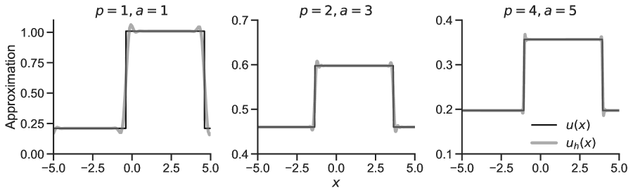
Figure 4: Tophat samples with varying degree $p$ and wave speed $a$, as indicated, generated for $\mathcal{C}^{0}$ discontinuity data with numerical DG approximations $u_{h}$ with their respective exact solutions $u$. Note the different vertical axis ranges.

We train the data-driven filter on linear, synthetic data as the nonlinear Euler test data is computationally expensive to solve. To remedy the differences in data distributions between the linear training and nonlinear test data, we cross-validate on a limited number of Euler samples that are time-evolved before the benchmark final times of the Euler test problems. The training data for the data-driven filter includes $\mathcal{C}^{0}$ discontinuities to represent the similar discontinuity types that arise in contact and shock discontinuities in Euler shock waves. The discontinuity data is extracted from DG numerical solutions to the linear advection equation, $u_{t}+au_{x}=0,\ u(x,0)=u_{0}(x)$, with wave speeds $a\in[1,5]$ and the top-hat or box wave initial condition,

$$u_{0}(x)=\begin{cases}\alpha+\delta,&x\in[-2.5,2.5]\\ \alpha,&\text{else}\end{cases},\quad x\in[-5,5].$$ (15)

A third-order strong stability-preserving Runge-Kutta scheme  [12, 42] is used to time-evolve the semi-discrete modal DG variational formulation [2, 4] of the linear PDE. The chosen wave speed values fall within the range of eigenvalues, $\lambda=\{u-c,u,u+c\}$, of the Euler test problems, as defined previously in Section 2.3. The numerical and exact solutions, $u_{h}$ and $u$, are generated for samples drawn uniformly from the following parameters: bias term $\alpha\in[0.1,0.5)$, jump parameter $\delta\in[0.1,1)$, DG degree $p\in\{1,2,3,4\}$, and final time $T_{f}\in\frac{|\Omega|}{a}\cdot[1.1,1.3)$. For this study, the training data includes a fixed discretization of $N=128$ elements ($h=\Delta x=10/128$) for $\Omega=[-5,5]$. Samples generated from this training data distribution are visualized in Fig. 4.

The training discontinuity data is extracted using troubled cell indication on the SIAC-filtered numerical solutions, $K_{H}\ast u_{h}=u_{h}^{\ast}$. We choose the threshold multiwavelet-based troubled cell indicator with a threshold value of $C=0.4$ [49, 48] to detect the discontinuity regions from the SIAC-filtered data. We note that other techniques may be used for troubled cell identification. The discontinuity training data comprises of the flagged troubled cell $TC_{i}$ and 4 cells to the left and right to define a troubled cell window $[TC_{i}-4,TC_{i}+4]$, as shown in the left of Fig. 5 for the samples from Fig. 4. Distinct troubled cells may flag the same discontinuity and thus the troubled cell window data is sorted to avoid discontinuities found at the edge of the troubled cell window and to also eliminate any troubled cells whose windows do not include $\mathcal{C}^{0}$ discontinuities. We evaluate the filtered data pointwise at 4 Gauss-Legendre quadrature nodes per element for all elements $[TC_{i}-4,TC_{i}+4]$, for an input data dimension of $36$ for the CNN. Quadrature nodes, rather than equispaced nodes, are chosen for the potential to extract DG modal information of the filtered data, with four quadrature nodes allowing data up to a degree-7 piecewise polynomial. A normalizing step is applied similar to what was done in [51], except that we normalize by the input data rather than the exact data, as the exact solution may not always be known in test data. For demonstration, the sorted, normalized discontinuity data is shown in Fig. 5 (right) and represent training data samples for the data-driven filter. The corresponding exact solution $u$ at those nodes is the true data to which the filtered output is compared, as in the objective function in Eq. 13. For this hybrid filter application, the training simulations include 900 top-hat samples with 100 samples for each wave speed $a\in\{1,1.5,2,\ldots,4.5,5\}$. With two discontinuities for each top-hat sample, and at least one troubled cell per discontinuity, the training data for the data-driven filter consists of 1,138 discontinuity window samples.

Figure 5: (Left) Window about troubled cell data including cells $[TC_{i}-4,TC_{i}+4]$ about 21 troubled cells $TC_{i}$ flagged from samples in Fig. 4 and (right) sorted and normalized discontinuity data to be used for NN training data.

A fixed network architecture along with one set of training parameters are used to determine $K_{\Theta}$. Five hidden convolutional layers are considered along with one input layer and one output layer with a kernel stencil of size 7. In addition, the layers are mapped to a hidden channel dimension of 128 and the activation function for each layer is the leaky ReLU, with a negative slope of 0.1. An Adam optimizer with a fixed learning rate of $10^{-4}$ is used to perform the stochastic gradient descent on the training data with a batch size of 200 [22]. The parameters $\Theta$ that achieve the lowest mean-squared error (MSE) loss on the validation dataset are the ones that are saved for $K_{\Theta}$. The validation dataset consists of 50 discontinuity samples from Euler Lax density samples from $T_{f}\in[0.7,1]$ and Sod density samples from $T_{f}\in[1,1.5]$. We note these do not lie in the training set distribution but are similar yet different from the testing set, which has samples drawn from later final times and includes the velocity and pressure variables as well as the sine-entropy initial condition. The reason for this choice of validation data is to ensure that there is no overfitting to the linear training data in order to have a a generalized filter that improves the approximation in discontinuous regions for the nonlinear test data. The limited sample size is due to the computational cost of the Euler simulations and also represents limited experimental data. The exact reference solutions for these Euler simulation samples are computed using the Clawpack Riemann solver, as used in [21].

4.2 The hybrid filtered approximation

As mentioned in Section 3.3, the hybrid filter is applied about troubled cell set windows that capture the discontinuity and its neighborhood. We consider troubled cell groupings $S_{i}$ with cells that are at most $n=4$ cells apart and padding by $d=4$ cells, as demonstrated in Fig. 3. Given the hybrid filter construction in Section 4.2, the hybrid filtered approximation comprises of a consistency-only SIAC filter about the discontinuity window $[\min(S_{i})-4,\ \max(S_{i})+4]$, except for the discontinuity cell $I_{j^{\dagger}}$, which is updated using the data-driven filter as follows,

$$K_{\Theta}\ast u_{h}^{*}\biggr{|}_{I_{j^{\dagger}}}=K_{\Theta}\ast(K_{H}\ast u_{h})\biggr{|}_{I_{j^{\dagger}}},$$

and its two adjacent cells $I_{j^{\dagger}\pm 1}$ are fitted using Hermite polynomial interpolation of degree $p^{H}=\min(p,2)$ using one data point from the discontinuity cell and $p^{H}$ data points from the neighboring cell $I_{j^{\dagger}\pm 2}$.

4.2.1 Hybrid-filtering Euler data

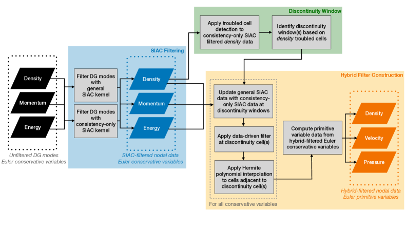
Figure 6: Process flow chart demonstrating the hybrid filter post-processing of solutions to Euler equations, from unfiltered conservative variable inputs to hybrid-filtered primitive variable outputs.

For solutions to Euler equations, the hybrid filter is applied to the conservative variables, which are then later used to determine the filtered primitive variables. The hybrid filter process for filtering the global solutions to Euler equations is demonstrated in Fig. 6, where first SIAC filtering is applied to the conservative variables. Next, the discontinuity windows are determined based on the consistency-only SIAC-filtered density variable. Density alone is found to be sufficient for multiwavelets-based troubled cell indication in [49], although other troubled cell indication methods require density and entropy or density and energy [36]. Hybrid-filtered entropy results can be found in Appendix A. While the density shock discontinuity yields $\mathcal{C}^{0}$ discontinuities for all Euler quantities, the density contact discontinuity yields smooth velocity and pressure profiles [20]. For all conservative variables (density, momentum, and energy), the global SIAC-filtered data is updated at the same discontinuity window(s) by the consistency-only SIAC-filtered data. Next, the data-driven filter is applied at the discontinuity cells $I_{j^{\dagger}}$, followed by Hermite polynomial interpolation in cells $I_{j^{\dagger}\pm 1}$. The filtered primitive variables (density, velocity, and pressure) are then computed using the hybrid filtered conservative variables in order to preserve the location of the contact and shock discontinuities.

5 Numerical Results

Table 1: The Lax grid $\ell_{2}$ and $\ell_{\infty}$ error quartiles for the unfiltered, SIAC moving average, and hybrid filter approximations about discontinuity windows from 84 Lax simulations drawn with final time $T_{f}\in[1,1.3]$, resulting in 142 discontinuity window samples, $[\min(S_{i})-4,\ \max(S_{i})+4]$. Hybrid filtered error values that are lower than the unfiltered data are shown in bold. Note: the velocity and pressure profiles are filtered in smooth regions where the density contact discontinuity is flagged as discontinuous.

Variable	Quartile	$\ell_{2}$ Error			$\ell_{\infty}$ Error
		Unfiltered	SIAC	Hybrid	Unfiltered	SIAC	Hybrid
Density	75%	2.01e-01	2.12e-01	1.81e-01	4.56e-01	4.50e-01	4.78e-01
	Median	1.68e-01	1.74e-01	4.80e-02	4.20e-01	4.16e-01	9.51e-02
	25%	1.48e-01	1.57e-01	2.36e-02	3.74e-01	3.75e-01	4.96e-02
Velocity	75%	3.25e-01	3.69e-01	8.76e-02	9.01e-01	9.70e-01	2.10e-01
	Median	2.73e-01	3.16e-01	4.65e-02	7.14e-01	8.11e-01	9.54e-02
	25%	9.06e-03	4.45e-03	5.19e-03	8.92e-03	5.09e-03	6.44e-03
Pressure	75%	3.41e-01	3.68e-01	8.01e-02	9.23e-01	9.14e-01	1.39e-01
	Median	2.90e-01	3.32e-01	3.43e-02	7.52e-01	7.64e-01	6.90e-02
	25%	1.35e-02	5.37e-03	6.24e-03	1.57e-02	5.89e-03	7.53e-03

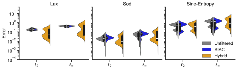
Figure 7: Euler density violinplots for the grid $\ell_{2}$ and $\ell_{\infty}$ error for the (left to right) Lax, Sod, and sine-entropy (Shu-Osher) datasets. In addition to the traditional box-and-whisker plot with the median shown in white, the violinplot shows the density of the errors by the width of the distribution plot, which is computed using a kernel density estimate.

The hybrid filter is tested on the following Euler problems: Lax [24], Sod [44], and sine-entropy or Shu-Osher [43] problems, as introduced in Section 2.3. All simulations, regardless of approximation order, are done using $N=128$ elements in $\Omega=[-5,5]$ up to or near the benchmark final times. Given the spurious oscillations that arise about the discontinuities in the three test problems, it is inevitable to consider troubled cell detection and slope limiting for the numerical solution to remain bounded. A TVB troubled cell detector [36] along with the Krivodonova moment limiter [23] are applied to the numerical simulations, though other choices are possible. Problem-dependent TVB parameters are considered to prevent instabilities in the numerical solutions, while keeping some spurious oscillations to test the effectiveness of the proposed filter. The simulation data are thus representative of noisy experimental data, with the proposed hybrid filter representing a post-processed solution of the experimental data.

Euler test data include single samples at final time and a compilation of simulation samples leading up to final time for the three benchmark problems. The Euler simulations include 84 Lax samples time-evolved to $T_{f}\in[1,1.3]$, 65 Sod samples with $T_{f}\in[1.5,2]$, and 84 sine-entropy (Shu-Osher) samples with $T_{f}\in[1,1.2]$. These were computed using a discontinuous Galerkin method on a mesh consisting of $N=128$ elements for polynomial degrees $p=1-4$ ($256,\,384,\,512,$ and $640$ degrees of freedom, respectively). The discontinuity detection method used herein results in 142 Lax, 85 Sod, and 91 sine-entropy discontinuity windows for each of the density, velocity, and pressure variables, which are then filtered using the hybrid filter as discussed in Section 4.2.1. For applications of the hybrid filter on the Euler entropy variable as well as different resolutions, the reader is directed to Appendix A-B, respectively.

We start off by presenting the performance of the hybrid filter across many samples in Section 5.1 to assess the overall effectiveness in reducing the error about discontinuities. In Sections 5.2-5.4, the hybrid filter is examined for individual samples of the Euler benchmark problems at final time. Specifically, we examine the filtered approximation about the discontinuity profiles and 1) how well the filter can resolve the location of the contact or shock discontinuity and 2) the error comparison to the unfiltered $\mathcal{O}(1)$ error band about the discontinuity.

5.1 Performance Assessment

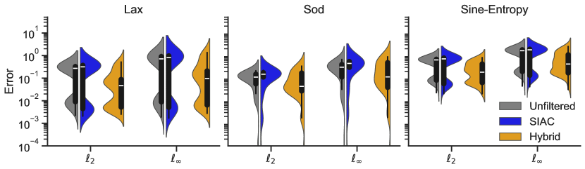
Figure 8: Euler velocity violinplots for the grid $\ell_{2}$ and $\ell_{\infty}$ error for the (left to right) Lax, Sod, and sine-entropy (Shu-Osher) datasets. In addition to the traditional box-and-whisker plot with the median shown in white, the violinplot shows the density of the errors by the width of the distribution plot, which is computed using a kernel density estimate.

Figure 9: Euler pressure violinplots for the grid $\ell_{2}$ and $\ell_{\infty}$ error for the (left to right) Lax, Sod, and sine-entropy (Shu-Osher) datasets. In addition to the traditional box-and-whisker plot with the median shown in white, the violinplot shows the density of the errors by the width of the distribution plot, which is computed using a kernel density estimate.

The performance of the proposed hybrid filter is first examined for discontinuity windows from the Euler test datasets. The filtered Lax data is presented in Table 1, which includes the quartiles for the grid $\ell_{2}$ and $\ell_{\infty}$ error for the unfiltered, SIAC-averaged or consistency-only SIAC filter, and the hybrid filter. The error quartiles for the hybrid filter that are lower than the unfiltered counterparts are reported in bold, highlighting an improvement for all quantities except for the 75th percentile for the density $\ell_{\infty}$ error. All median error values across density, velocity, and pressure variables are lowered with the hybrid filter.

To visualize the distribution of the error across all three Euler test datasets, violinplots are presented in Fig. 7-9 for density, velocity, and pressure, respectively. The violinplots include the traditional box-and-whisker plot with the median or 50% quartile shown in white inside the box, along with a kernel density estimate (KDE) or a kernel-smoothened probability density estimation of the underlying distribution of the error data. Across all figures (Fig. 7-9) capturing three test problems and three variables, the median is lower for the hybrid filtered data compared to the unfiltered and SIAC-filtered approximations. The KDE highlights a lower error distribution for all Lax samples (left plots in Fig. 7-9). For the Sod problem (center plots), there is a smaller shift towards lower error values compared to the unfiltered and SIAC-filtered data, as shown by the KDE, but it is worth noting that the unfiltered error is lowest compared to the Lax and sine-entropy problems. Other than the velocity profile, the Sod error is in the order of $10^{-1}$ and not $\mathcal{O}(1)$, as is common for $\mathcal{C}^{0}$ discontinuities. The sine-entropy density profile is the most challenging discontinuity, with a shock about high-to-low frequency sinusoidals. While the hybrid filter reduces the median error for such a complex discontinuity, it particularly improves on the velocity and pressure shocks, which include a discontinuity about piecewise sinusoidal to constant data.

5.2 Lax Samples at Final Time

The Lax problem includes two discontinuities of interest: the density contact discontinuity about $x=2$ and the density shock discontinuity about $x=3.1$. The former is challenging to resolve given the large discontinuity jump in the density approximation, which is often poorly resolved in existing numerical methods. The application of our hybrid filtered approach at this contact discontinuity is shown in Fig. 10 for a DG degree 2 approximation. The hybrid filter precisely locates the contact discontinuity, and this is also achieved for the degree 4 approximation as noted by the significant reduction in the $\ell_{\infty}$ error in Table 2. While the contact discontinuity is not detected for the degree 3 approximation, which relies on the troubled-cell indicator, all other degree approximations are improved in the $\ell_{2}$ error and degrees $p>2$ reduce the $\ell_{\infty}$ error. The $\mathcal{O}(1)$ error band, as shown on the right of Fig. 10, is flattened, yielding errors of $\mathcal{O}(10^{-1})$. The Lax shock discontinuity for the degree 2 approximation is presented in Fig. 11, which also shows precise location extraction. In contrast to the contact discontinuity, the hybrid filter applied to the degree 1 approximation yields an $\ell_{\infty}$ error reduction that is close to one order of magnitude, from $3.75\times 10^{-1}$ down to $6.78\times 10^{-2}$, as listed in Table 2. Although the hybrid filtered degree 2-4 approximations have less significant error reduction compared to degree 1, they achieve lower errors when compared to the reference solution in the location of the shock.

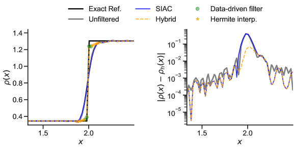
Figure 10: Lax density contact discontinuity at final time $T_{f}=1.3$ with DG degree 2 data: (right) unfiltered (gray), SIAC moving average filter (blue), and hybrid filter (yellow dashed) approximations, including where the data-driven filter (green dots) and Hermite polynomial interpolation (yellow stars) are applied. The left plot shows the pointwise error for the respective filtered approximations.

Table 2: Lax density grid $\ell_{2}$ and $\ell_{\infty}$ error for the density contact and shock discontinuities at final time $T_{f}=1.3$ about discontinuity windows, $[\min(S_{i})-4,\ \max(S_{i})+4]$.

Degree	Approx.	Contact		Shock
		$\ell_{2}$	$\ell_{\infty}$	$\ell_{2}$	$\ell_{\infty}$
$p=1$	Unfiltered	2.62e-01	4.55e-01	1.50e-01	3.75e-01
	SIAC	2.64e-01	4.55e-01	1.53e-01	3.89e-01
	Hybrid	2.25e-01	7.30e-01	3.75e-02	6.78e-02
$p=2$	Unfiltered	1.93e-01	3.99e-01	1.44e-01	3.86e-01
	SIAC	2.03e-01	3.97e-01	1.60e-01	4.15e-01
	Hybrid	3.99e-02	6.64e-02	1.06e-01	3.75e-01
$p=3$	Unfiltered	-	-	1.50e-01	3.92e-01
	SIAC	-	-	1.60e-01	4.17e-01
	Hybrid	-	-	1.20e-01	4.27e-01
$p=4$	Unfiltered	1.84e-01	3.81e-01	1.53e-01	3.87e-01
	SIAC	1.94e-01	3.84e-01	1.63e-01	4.14e-01
	Hybrid	3.82e-02	5.88e-02	9.57e-02	3.37e-01

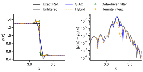
Figure 11: Lax density shock discontinuity at final time $T_{f}=1.3$ with DG degree 2 data: (right) unfiltered (gray), SIAC moving average filter (blue), and hybrid filter (yellow dashed) approximations, including where the data-driven filter (green dots) and Hermite polynomial interpolation (yellow stars) are applied. The left plot shows the pointwise error for the respective filtered approximations.

5.3 Sod Samples at Final Time

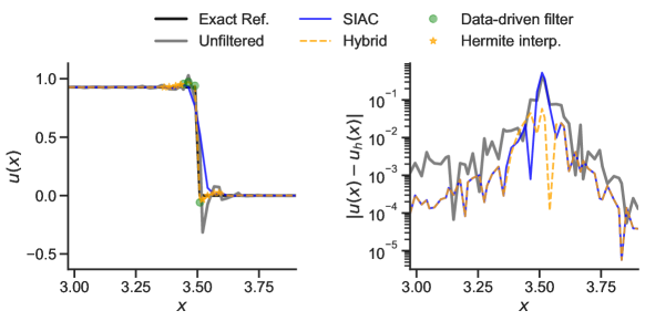
Figure 13: Sod velocity at the density shock discontinuity at final time $T_{f}=2$ with DG degree 2 data: (right) unfiltered (gray), SIAC moving average filter (blue), and hybrid filter (yellow dashed) approximations, including where the data-driven filter (green dots) and Hermite polynomial interpolation (yellow stars) are applied. The left plot shows the pointwise error for the respective filtered approximations.

For the Sod problem, we examine the hybrid filter performance on the velocity data. Although the contact discontinuity represents a $\mathcal{C}^{0}$ discontinuity for the density profile alone, we present the hybrid filtered approximation about the smooth, constant velocity data where the density contact is located to illustrate the filter’s capacity to reproduce constant data, as enforced by the consistency constraint. Figure 12 shows that the hybrid filter maintains the constant data and additionally reduces the error. In fact, the error in Table 3 shows that the hybrid filter can maintain the SIAC filtered $\ell_{2}$ and $\ell_{\infty}$ error and the SIAC filter performs better for this contact discontinuity. As for the Sod shock discontinuity, the velocity profile has a $\mathcal{C}^{0}$ discontinuity, which benefits from the hybrid filter which can extract the precise location of the shock as shown by the degree 2 data in Fig. 13. The shock $\ell_{2}$ and $\ell_{\infty}$ error values, as shown in Table 3, are reduced by about one order of magnitude with the hybrid filter for all degree approximations.

5.4 Sine-Entropy (Shu-Osher) Samples at Final Time

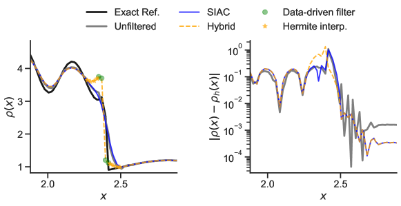
Figure 14: Sine-entropy (Shu-Osher) density at the density shock discontinuity at final time $T_{f}=1.8$ with DG degree 2 data: (right) unfiltered (gray), SIAC moving average filter (blue), and hybrid filter (yellow dashed) approximations, including where the data-driven filter (green dots) and Hermite polynomial interpolation (yellow stars) are applied. The left plot shows the pointwise error for the respective filtered approximations.

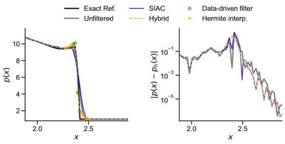
Figure 15: Sine-entropy (Shu-Osher) pressure at the density shock discontinuity at final time $T_{f}=1.8$ with DG degree 2 data: (right) unfiltered (gray), SIAC moving average filter (blue), and hybrid filter (yellow dashed) approximations, including where the data-driven filter (green dots) and Hermite polynomial interpolation (yellow stars) are applied. The left plot shows the pointwise error for the respective filtered approximations.

The sine-entropy or Shu-Osher problem has a strong shock, which we demonstrate here for both the density and pressure profiles. The discontinuity for the density profile includes a shock about high-to-low frequency sinusoidal waves, with the degree 2 results presented in Fig. 14. The $\ell_{2}$ and $\ell_{\infty}$ errors included in Table 4 show that the SIAC filter performs better than the hybrid filter in reducing the $\ell_{\infty}$ error across all degrees and the unfiltered density data has the lowest $\ell_{2}$ error. However, the hybrid-filtered data presented in Fig. 14 is more accurate to the right of the shock given that the data-driven filter resolves the bottom of the shock. In addition, the sine-entropy simulations are coarser than what would typically be considered ($N=128$ elements instead of $N=256$), but these filtered outcomes show that more details can be extracted from the coarse data of the shock discontinuity. We expect the performance to be further improved with better resolution, as presented in the multi-resolution Lax filter results in Appendix B. The pressure profile for the sine-entropy problem is piecewise sinusoidal to constant, as shown in Fig. 15, which shows that the location of the discontinuity is resolved. The error values in Table 4 indicate that the hybrid filter performs well in the $\ell_{2}$ and $\ell_{\infty}$ error for the degree 2 and 3 approximations while the SIAC filter improves the $\ell_{\infty}$ error for the other degrees.

6 Discussion and Future Work

In this work, we present a hybrid filter for discontinuities using an adapted SIAC kernel fused with data-driven and interpolation methods. This hybrid post-processing filter reduces the $\mathcal{O}(1)$ error about $\mathcal{C}^{0}$ discontinuities, which have thus far not been possible with post-processing filter techniques. Specifically, this discontinuity-targeted hybrid filter is able to locate the vertical slope in the data by learning on simply top-hat data for $\mathcal{C}^{0}$ discontinuity profiles. The Lax and Sod shock discontinuities are precisely located across all variables (density, velocity, and pressure) except for the Lax density shock which is partially resolved, allowing for sub-cell feature extraction. The contact discontinuity is well captured for the Lax problem, which is the most challenging discontinuity to refine, and the Sod contact discontinuity for the constant velocity data highlights the enforced consistency constraint for the data-driven filter. Additionally, the complex sinusoidal shock in the sine-entropy (Shu-Osher) problem is improved to the right of the shock discontinuity with this hybrid filter method, despite the nonlinear nature and coarse simulation data. Generally, the hybrid filter performs better for higher-order data, but all data experience narrowing or flattening of the $\mathcal{O}(1)$ error band near discontinuities.

Future work involves improving the hybrid, SIAC – data-driven filter to be effective across different problems. This includes low-order and high-order approximations as well as the discontinuity precision for the sine-entropy problem. Additionally, while this particular hybrid filter application is for final time post-processing, this hybrid filter can be applied at each time step in a time-evolving scheme for a more robust limiter application. The methods used herein to identify the discontinuity windows and to merge hybrid techniques to extract accuracy at the discontinuity can be leveraged to improve the numerical approximation at each time step. Finally, since our current architecture only allows for kernel consistency constraints, we will explore the use of optimization-based implicit neural network architectures [14] to embed additional physical constraints.

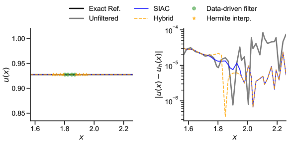
Figure 12: Sod velocity at the density contact discontinuity at final time $T_{f}=2$ with DG degree 2 data: (right) unfiltered (gray), SIAC moving average filter (blue), and hybrid filter (yellow dashed) approximations, including where the data-driven filter (green dots) and Hermite polynomial interpolation (yellow stars) are applied. The left plot shows the pointwise error for the respective filtered approximations.

Table 3: Sod velocity grid $\ell_{2}$ and $\ell_{\infty}$ error for the density contact and shock discontinuities at final time $T_{f}=2$ about discontinuity windows, $[\min(S_{i})-4,\ \max(S_{i})+4]$. Note: the Sod velocity profile has a $\mathcal{C}^{0}$ discontinuity at the shock and not at the density contact discontinuity; the error values at the contact are thus shown in italics.

Degree	Approx.	Contact		Shock
		$\ell_{2}$	$\ell_{\infty}$	$\ell_{2}$	$\ell_{\infty}$
$p=1$	Unfiltered	5.73e-05	6.88e-05	1.78e-01	5.37e-01
	SIAC	5.49e-05	6.43e-05	1.85e-01	4.80e-01
	Hybrid	5.90e-05	7.18e-05	3.66e-02	4.88e-02
$p=2$	Unfiltered	5.78e-05	8.37e-05	1.54e-01	4.04e-01
	SIAC	2.55e-05	3.06e-05	1.87e-01	5.29e-01
	Hybrid	2.63e-05	3.06e-05	2.76e-02	5.84e-02
$p=3$	Unfiltered	-	-	1.50e-01	4.45e-01
	SIAC	-	-	2.00e-01	5.60e-01
	Hybrid	-	-	1.72e-02	4.69e-02
$p=4$	Unfiltered	8.58e-03	1.02e-02	8.44e-02	2.67e-01
	SIAC	2.21e-03	3.03e-03	2.05e-01	5.71e-01
	Hybrid	1.97e-03	3.03e-03	1.69e-02	3.73e-02

Appendix A Filtering the Entropy Variable

The entropy variable is another key Euler quantity that can be further examined and utilized for discontinuity detection [48]. Similar to the primitive variables (velocity and pressure), filtering of the entropy variable can be achieved by first filtering the conservative variables and then evaluating the related quantities, as demonstrated in Section 4.2.1. The following entropy variable is considered,

$$S=\frac{p}{\rho^{\gamma}}.$$

To examine the filtered entropy data, first filtering of density $\rho$, momentum $\rho u$, and energy $E$ is applied, then the filtered pressure $p=(\gamma-1)(E-\frac{1}{2}\rho u^{2})$ is evaluated from the filtered conservative variables, and finally filtered entropy $S$ can be computed. The Lax entropy data is examined herein at the density contact and shock discontinuities.

The entropy data has an error profile of $\mathcal{O}(10)$ at the density contact discontinuity, as shown in the DG degree 2 data in Fig. 16 and in Table 5. Despite the hybrid filter’s capacity to handle smaller error profiles, the hybrid filtered entropy data shows the precise discontinuity location, as shown in Fig. 16.

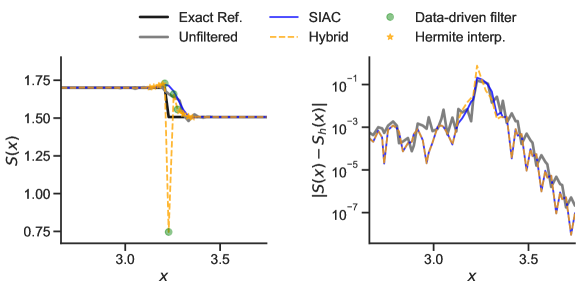
Figure 17: Lax entropy at the density shock discontinuity at final time $T_{f}=1.3$ with DG degree 2 data: (right) unfiltered (gray), SIAC moving average filter (blue), and hybrid filter (yellow dashed) approximations, including where the data-driven filter (green dots) and Hermite polynomial interpolation (yellow stars) are applied. The left plot shows the pointwise error for the respective filtered approximations.

In contrast, the entropy data for the shock discontinuity is of $\mathcal{O}(10^{-1})$, 100$\times$ smaller than entropy at the density contact discontinuity. While the location of the discontinuity at the shock is extracted, there are more significant undershoots of the data, as shown in Fig. 17, resulting in the larger $\ell_{2}$ and $\ell_{\infty}$ error, as reported in Table 5. The SIAC filter performs better for most cases and [33] shows that it is promising for entropy correction.

Appendix B Multi-resolution Hybrid Filters

Although the hybrid filter was constructed for DG numerical data evaluated at $N=128$ elements in a domain $\Omega=[-5,5]$, we test the performance of the hybrid filter at coarser ($N=64$) and finer ($N=256$) resolutions for the Lax problem. We expect the Sod problem to be similar, but the Lax problem poses more challenging discontinuities and so does the sine-entropy problem. Similar to Section 5.2, we present here the filter results for the Lax density data at the contact and shock discontinuities. The discontinuity windows (Section 3.3) for coarser data with $N=64$ elements were adapted to group troubled cells that are at most $n=2$ cells apart and with padding by $d=2$ cells on each side for a filter evaluation window of $[\min(S_{i})-2,\ \max(S_{i})+2]$. The discontinuity window parameters for finer data with $N=256$ elements were the same as those with $N=128$ elements. The hybrid filter construction is the same as defined in Section 4.2.

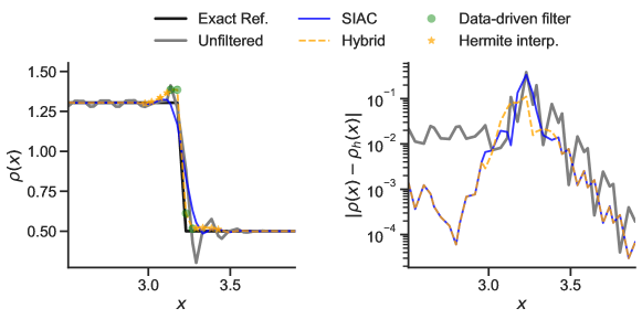
Figure 19: Coarser ($N=64$) Lax density shock discontinuity at final time $T_{f}=1.3$ with DG degree 2 data: (right) unfiltered (gray), SIAC moving average filter (blue), and hybrid filter (yellow dashed) approximations, including where the data-driven filter (green dots) and Hermite polynomial interpolation (yellow stars) are applied. The left plot shows the pointwise error for the respective filtered approximations.

For coarse data, the degree 2 filtered results for the contact discontinuity are presented in Fig. 18 and the shock discontinuity are presented in Fig. 19. Both filtering outputs show an error reduction of the $\mathcal{O}(1)$ error band. The grid $\ell_{2}$ and $\ell_{\infty}$ errors (Table 6) are improved for degree 2. The hybrid filter improves the $\ell_{2}$ and $\ell_{\infty}$ error for the shock discontinuity for the degree 1-3 approximations but only improves the contact discontinuity in the $\ell_{2}$ error for degree 1 and in the $\ell_{2}$ and $\ell_{\infty}$ error for degree 2.

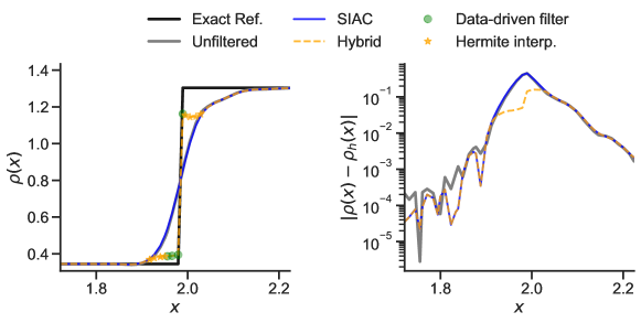
Figure 20: Finer ($N=256$) Lax density contact discontinuity at final time $T_{f}=1.3$ with DG degree 2 data: (right) unfiltered (gray), SIAC moving average filter (blue), and hybrid filter (yellow dashed) approximations, including where the data-driven filter (green dots) and Hermite polynomial interpolation (yellow stars) are applied. The left plot shows the pointwise error for the respective filtered approximations.

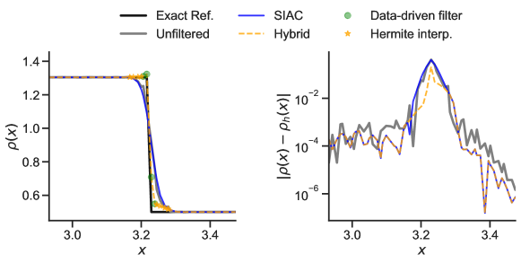
Figure 21: Finer ($N=256$) Lax density shock discontinuity for DG degree 2 data: (right) unfiltered (gray), SIAC moving average filter (blue), and hybrid filter (yellow dashed) approximations, including where the data-driven filter (green dots) and Hermite polynomial interpolation (yellow stars) are applied. The left plot shows the pointwise error for the respective filtered approximations.

A resolution with $N=256$ elements is considered to examine the performance of the hybrid filter at finer resolutions. The degree 2 filtered data demonstrates precise contact (Fig. 20) and shock (Fig. 21) discontinuity location and feature extraction. Additionally, the $\ell_{2}$ and $\ell_{\infty}$ error values in Table 7 demonstrate an error reduction for all degrees 1-4 where the discontinuities are detected.

Table 4: Sine-entropy (Shu-Osher) density and pressure grid $\ell_{2}$ and $\ell_{\infty}$ error for the strong shock discontinuity at final time $T_{f}=1.8$ about discontinuity window, $[\min(S_{i})-4,\ \max(S_{i})+4]$.

Degree	Approx.	Density		Pressure
		$\ell_{2}$	$\ell_{\infty}$	$\ell_{2}$	$\ell_{\infty}$
$p=1$	Unfiltered	3.98e-01	9.75e-01	1.03e+00	3.21e+00
	SIAC	4.10e-01	8.40e-01	1.20e+00	3.10e+00
	Hybrid	5.81e-01	1.36e+00	1.24e+00	4.13e+00
$p=2$	Unfiltered	4.18e-01	1.09e+00	1.26e+00	3.77e+00
	SIAC	4.39e-01	1.02e+00	1.40e+00	3.66e+00
	Hybrid	5.47e-01	1.33e+00	7.66e-01	2.35e+00
$p=3$	Unfiltered	4.08e-01	1.15e+00	1.22e+00	3.88e+00
	SIAC	4.16e-01	9.80e-01	1.36e+00	3.58e+00
	Hybrid	5.28e-01	1.24e+00	7.89e-01	2.66e+00
$p=4$	Unfiltered	3.80e-01	1.12e+00	1.12e+00	3.74e+00
	SIAC	4.00e-01	9.63e-01	1.31e+00	3.50e+00
	Hybrid	5.20e-01	1.23e+00	1.28e+00	4.51e+00

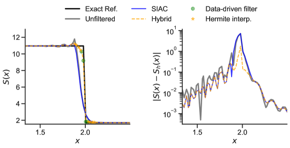
Figure 16: Lax entropy at the density contact discontinuity at final time $T_{f}=1.3$ with DG degree 2 data: (right) unfiltered (gray), SIAC moving average filter (blue), and hybrid filter (yellow dashed) approximations, including where the data-driven filter (green dots) and Hermite polynomial interpolation (yellow stars) are applied. The left plot shows the pointwise error for the respective filtered approximations.

Table 5: Lax $\boldsymbol{N=128}$ entropy grid $\ell_{2}$ and $\ell_{\infty}$ error for the density contact and shock discontinuities at final time $T_{f}=1.3$ about discontinuity windows, $[\min(S_{i})-4,\ \max(S_{i})+4]$.

Degree	Approx.	Contact		Shock
		$\ell_{2}$	$\ell_{\infty}$	$\ell_{2}$	$\ell_{\infty}$
$p=1$	Unfiltered	5.35e+00	7.52e+00	6.35e-02	1.81e-01
	SIAC	5.00e+00	7.58e+00	9.96e-02	2.33e-01
	Hybrid	3.99e+00	8.72e+00	6.85e-02	2.19e-01
$p=2$	Unfiltered	3.02e+00	7.17e+00	7.30e-02	1.53e-01
	SIAC	3.15e+00	7.22e+00	8.81e-02	2.08e-01
	Hybrid	5.71e-01	1.78e+00	2.18e-01	7.61e-01
$p=3$	Unfiltered	-	-	7.50e-02	1.85e-01
	SIAC	-	-	9.39e-02	2.23e-01
	Hybrid	-	-	2.24e-01	7.75e-01
$p=4$	Unfiltered	2.83e+00	7.09e+00	7.48e-02	1.80e-01
	SIAC	2.98e+00	7.11e+00	9.12e-02	2.22e-01
	Hybrid	4.86e-01	1.68e+00	1.99e-01	6.88e-01

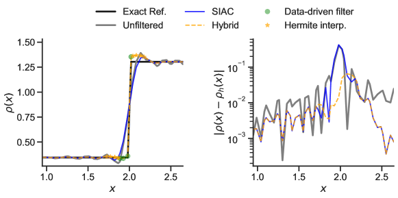
Figure 18: Coarser ($N=64$) Lax density contact discontinuity at final time $T_{f}=1.3$ with DG degree 2 data: (right) unfiltered (gray), SIAC moving average filter (blue), and hybrid filter (yellow dashed) approximations, including where the data-driven filter (green dots) and Hermite polynomial interpolation (yellow stars) are applied. The left plot shows the pointwise error for the respective filtered approximations.

Table 6: Coarser ($N=64$) Lax density grid $\ell_{2}$ and $\ell_{\infty}$ error for the density contact and shock discontinuities at final time $T_{f}=1.3$ about discontinuity windows, $[\min(S_{i})-2,\ \max(S_{i})+2]$.

Degree	Approx.	Contact		Shock
		$\ell_{2}$	$\ell_{\infty}$	$\ell_{2}$	$\ell_{\infty}$
$p=1$	Unfiltered	3.48e-01	4.93e-01	1.91e-01	3.75e-01
	SIAC	3.53e-01	4.94e-01	1.71e-01	3.47e-01
	Hybrid	3.34e-01	7.93e-01	7.62e-02	9.91e-02
$p=2$	Unfiltered	2.30e-01	4.06e-01	1.85e-01	3.84e-01
	SIAC	2.40e-01	4.23e-01	1.55e-01	3.38e-01
	Hybrid	5.45e-02	6.46e-02	7.10e-02	1.12e-01
$p=3$	Unfiltered	-	-	1.82e-01	3.80e-01
	SIAC	-	-	1.71e-01	3.68e-01
	Hybrid	-	-	1.13e-01	2.62e-01
$p=4$	Unfiltered	2.69e-01	4.72e-01	1.91e-01	4.61e-01
	SIAC	2.83e-01	4.50e-01	2.11e-01	4.39e-01
	Hybrid	2.77e-01	6.81e-01	3.03e-01	7.62e-01

Table 7: Finer ($N=256$) Lax density grid $\ell_{2}$ and $\ell_{\infty}$ error for the density contact and shock discontinuities at final time $T_{f}=1.3$ about discontinuity windows, $[\min(S_{i})-4,\ \max(S_{i})+4]$.

Degree	Approx.	Contact		Shock
		$\ell_{2}$	$\ell_{\infty}$	$\ell_{2}$	$\ell_{\infty}$
$p=1$	Unfiltered	2.11e-01	4.82e-01	1.07e-01	4.18e-01
	SIAC	2.14e-01	4.83e-01	1.11e-01	3.98e-01
	Hybrid	1.33e-01	3.02e-01	3.83e-02	1.77e-01
$p=2$	Unfiltered	1.81e-01	4.49e-01	1.09e-01	4.14e-01
	SIAC	1.86e-01	4.50e-01	1.17e-01	4.05e-01
	Hybrid	8.33e-02	1.59e-01	4.45e-02	2.09e-01
$p=3$	Unfiltered	-	-	1.07e-01	4.12e-01
	SIAC	-	-	1.15e-01	4.07e-01
	Hybrid	-	-	4.98e-02	2.37e-01
$p=4$	Unfiltered	1.78e-01	4.54e-01	1.10e-01	4.16e-01
	SIAC	1.84e-01	4.60e-01	1.16e-01	4.08e-01
	Hybrid	8.42e-02	1.65e-01	4.92e-02	2.33e-01

References

- [1] J. H. Bramble and A. H. Schatz, Higher order local accuracy by averaging in the finite element method, Mathematics of Computation, 31 (1977), pp. 94–111.
- [2] B. Cockburn, Discontinuous Galerkin Methods for Convection-Dominated Problems, Springer Berlin Heidelberg, Berlin, Heidelberg, 1999, pp. 69–224.
- [3] B. Cockburn, M. Luskin, C.-W. Shu, and E. Süli, Enhanced accuracy by post-processing for finite element methods for hyperbolic equations, Mathematics of Computation, 72 (2003), pp. 577–606.
- [4] B. Cockburn and C.-W. Shu, Runge–Kutta discontinuous Galerkin methods for convection-dominated problems, Journal of Scientific Computing, 16 (2001), p. 173–261.
- [5] S. Curtis, R. M. Kirby, J. K. Ryan, and C.-W. Shu, Postprocessing for the discontinuous Galerkin method over nonuniform meshes, SIAM Journal on Scientific Computing, 30 (2008), pp. 272–289.
- [6] M. Danelljan, A. Robinson, F. Shahbaz Khan, and M. Felsberg, Beyond correlation filters: Learning continuous convolution operators for visual tracking, in Computer Vision – ECCV 2016, B. Leibe, J. Matas, N. Sebe, and M. Welling, eds., Cham, 2016, Springer International Publishing, pp. 472–488.
- [7] A. Dedner, J. Giesselmann, T. Pryer, and J. Ryan, Residual estimates for post-processors in elliptic problems, SIAM Journal on Scientific Computing, 88 (2021).
- [8] J. Docampo-Sánchez, J. K. Ryan, M. Mirzargar, and R. M. Kirby, Multi-dimensional filtering: Reducing the dimension through rotation, SIAM Journal on Scientific Computing, 39 (2017), pp. A2179–A2200.
- [9] J. Docampo-Sánchez, G. Jacobs, X. Li, and J. Ryan, Enhancing accuracy with a convolution filter: What works and why!, Computers & fluids, 213 (2020), pp. 104727–.
- [10] R. L. Dougherty, A. Edelman, and J. M. Hyman, Nonnegativity-, monotonicity-, or convexity-preserving cubic and quintic hermite interpolation, Math. Comput.; (United States), 52 (1989), pp. 471–494.
- [11] S. W. Fung, H. Heaton, Q. Li, D. McKenzie, S. Osher, and W. Yin, Jfb: Jacobian-free backpropagation for implicit networks, in Proceedings of the AAAI Conference on Artificial Intelligence, vol. 36, 2022, pp. 6648–6656.
- [12] S. Gottlieb and C.-W. Shu, Total variation diminishing Runge-Kutta schemes, Mathematics of Computation, 67 (1998), pp. 73–85.
- [13] K. Han, Y. Wang, C. Xu, C. Xu, E. Wu, and D. Tao, Learning versatile convolution filters for efficient visual recognition, IEEE Transactions on Pattern Analysis and Machine Intelligence, 44 (2022), pp. 7731–7746.
- [14] H. Heaton and S. W. Fung, Explainable AI via learning to optimize, arXiv preprint arXiv:2204.14174, (2022).
- [15] H. Heaton, S. Wu Fung, A. Gibali, and W. Yin, Feasibility-based fixed point networks, Fixed Point Theory and Algorithms for Sciences and Engineering, 2021 (2021), pp. 1–19.
- [16] J. Hesthaven, Chapter 17 - Spectral Methods for Hyperbolic Problems, in Handbook of Numerical Methods for Hyperbolic Problems, R. Abgrall and C.-W. Shu, eds., vol. 17 of Handbook of Numerical Analysis, Elsevier, 2016, pp. 441–466.
- [17] J. S. Hesthaven, S. Gottlieb, and D. Gottlieb, Spectral Methods for Time-Dependent Problems, Cambridge Monographs on Applied and Computational Mathematics, Cambridge University Press, 2007.
- [18] X. Hu, W. Liu, and H. Huo, An intelligent network traffic prediction method based on butterworth filter and cnn–lstm, Computer Networks, 240 (2024), p. 110172.
- [19] A. D. Jagtap, E. Kharazmi, and G. E. Karniadakis, Conservative Physics-Informed Neural Networks on discrete domains for conservation laws: Applications to forward and inverse problems, Computer Methods in Applied Mechanics and Engineering, 365 (2020), p. 113028.
- [20] A. Jeffrey, A note on the derivation of the discontinuity conditions across contact discontinuities, shocks and phase fronts, Journal of Applied Mathematics and Physics (ZAMP), 15 (1964), p. 68–71.
- [21] D. I. Ketcheson, R. J. LeVeque, and M. J. del Razo, Riemann Problems and Jupyter Solutions, Society for Industrial and Applied Mathematics, Philadelphia, PA, 2020.
- [22] D. P. Kingma and J. Ba, Adam: A method for stochastic optimization, arXiv preprint arXiv:1412.6980, (2014).
- [23] L. Krivodonova, Limiters for high-order discontinuous Galerkin methods, Journal of Computational Physics, 226 (2007), pp. 879–896.
- [24] P. D. Lax, Weak solutions of nonlinear hyperbolic equations and their numerical computation, Communications on Pure and Applied Mathematics, 7 (1954), pp. 159–193.
- [25] R. J. LeVeque, Numerical Methods for Conservation Laws, Lectures in Mathematics, Birkhäuser, Basel, 2 ed., 1992.
- [26] H. Liang, Z. Song, C. Zhao, and X. Bian, Continuous and discontinuous compressible flows in a converging–diverging channel solved by Physics-Informed Neural Networks without exogenous data, Scientific Reports, 14 (2024).
- [27] L. Liu, S. Liu, H. Xie, F. Xiong, T. Yu, M. Xiao, L. Liu, and H. Yong, Discontinuity computing using Physics-Informed Neural Network, arXiv:2206.03864, (2022).
- [28] Z. Mao, A. D. Jagtap, and G. E. Karniadakis, Physics-Informed Neural Networks for high-speed flows, Computer Methods in Applied Mechanics and Engineering, 360 (2020), p. 112789.
- [29] D. McKenzie, S. W. Fung, and H. Heaton, Faster predict-and-optimize with three-operator splitting, arXiv preprint arXiv:2301.13395, (2023).
- [30] D. McKenzie, H. Heaton, Q. Li, S. Wu Fung, S. Osher, and W. Yin, Three-operator splitting for learning to predict equilibria in convex games, SIAM Journal on Mathematics of Data Science, 6 (2024), pp. 627–648.
- [31] M. Mirzargar, A. Jallepalli, J. K. Ryan, and R. M. Kirby, Hexagonal smoothness-increasing accuracy-conserving filtering, J. Sci. Comput., 73 (2017), p. 1072–1093.
- [32] M. S. Mock and P. D. Lax, The computation of discontinuous solutions of linear hyperbolic equations, Communications on Pure and Applied Mathematics, 31 (1978), pp. 423–430.
- [33] M. J. Picklo and A. K. Edoh, High-order entropy correction with siac filters, 2023.
- [34] M. J. Picklo and J. K. Ryan, Enhanced multiresolution analysis for multidimensional data utilizing line filtering techniques, SIAM Journal on Scientific Computing, 44 (2022), pp. A2628–A2650.
- [35] J. Qiu and C.-W. Shu, Hermite WENO schemes and their application as limiters for Runge–Kutta discontinuous Galerkin method: one-dimensional case, Journal of Computational Physics, 193 (2004), pp. 115–135.
- [36] J. Qiu and C.-W. Shu, A comparison of troubled-cell indicators for Runge–Kutta discontinuous Galerkin methods using weighted essentially nonoscillatory limiters, SIAM Journal on Scientific Computing, 27 (2005), pp. 995–1013.
- [37] J. Qu, W. Cai, and Y. Zhao, Learning time-dependent PDEs with a linear and nonlinear separate convolutional neural network, Journal of Computational Physics, 453 (2022), p. 110928.
- [38] M. Raissi, P. Perdikaris, and G. Karniadakis, Physics-Informed Neural Networks: A deep learning framework for solving forward and inverse problems involving nonlinear partial differential equations, Journal of Computational Physics, 378 (2019), pp. 686–707.
- [39] D. Ray and J. S. Hesthaven, An artificial neural network as a troubled-cell indicator, Journal of Computational Physics, 367 (2018), pp. 166 – 191.
- [40] D. Ray and J. S. Hesthaven, Detecting troubled-cells on two-dimensional unstructured grids using a neural network, Journal of Computational Physics, 397 (2019), p. 108845.
- [41] J. Ryan, C.-W. Shu, and H. Atkins, Extension of a post processing technique for the discontinuous Galerkin method for hyperbolic equations with application to an aeroacoustic problem, SIAM Journal on Scientific Computing, 26 (2005), pp. 821–843.
- [42] C.-W. Shu and S. Osher, Efficient implementation of essentially non-oscillatory shock-capturing schemes, Journal of Computational Physics, 77 (1988), pp. 439–471.
- [43] C.-W. Shu and S. Osher, Efficient implementation of essentially non-oscillatory shock-capturing schemes, ii, Journal of computational physics, 83 (1989), pp. 32–78.
- [44] G. A. Sod, A survey of several finite difference methods for systems of nonlinear hyperbolic conservation laws, Journal of Computational Physics, 27 (1978), pp. 1–31.
- [45] E. F. Toro, Riemann Solvers and Numerical Methods for Fluid Dynamics: A Practical Introduction, Springer, Berlin, Heidelberg, 3 ed., 2009.
- [46] S. ur Rehman, S. Tu, M. Waqas, Y. Huang, O. ur Rehman, B. Ahmad, and S. Ahmad, Unsupervised pre-trained filter learning approach for efficient convolution neural network, Neurocomputing, 365 (2019), pp. 171–190.
- [47] H. Vandeven, Family of spectral filters for discontinuous problems, Journal of Scientific Computing, 6 (1991), pp. 159–192.
- [48] M. J. Vuik, Multiwavelets and outlier detection for troubled-cell indication in discontinuous Galerkin methods, Ph.D. dissertation, Delft University of Technology, 2017.
- [49] M. J. Vuik and J. K. Ryan, Multiwavelet troubled-cell indicator for discontinuity detection of discontinuous Galerkin schemes, Journal of Computational Physics, 270 (2014), pp. 138–160.
- [50] M. J. Vuik and J. K. Ryan, Automated parameters for troubled-cell indicators using outlier detection, SIAM Journal on Scientific Computing, 38 (2016), pp. A84–A104.
- [51] X. Wen, W. S. Don, Z. Gao, and J. Hesthaven, An edge detector based on artificial neural network with application to hybrid compact-WENO finite difference scheme, Journal of Scientific Computing, 83 (2020).