Beyond Closure Models: Learning Chaotic-Systems via Physics-Informed Neural Operators

Abstract

Accurately predicting the long-term behavior of chaotic systems is crucial for various applications such as climate modeling. However, achieving such predictions typically requires iterative computations over a dense spatiotemporal grid to account for the unstable nature of chaotic systems, which is expensive and impractical in many real-world situations. An alternative approach to such a full-resolved simulation is using a coarse grid and then correcting its errors through a closure model, which approximates the overall information from fine scales not captured in the coarse-grid simulation. Recently, ML approaches have been used for closure modeling, but they typically require a large number of training samples from expensive fully-resolved simulations (FRS). In this work, we prove an even more fundamental limitation, i.e., the standard approach to learning closure models suffers from a large approximation error for generic problems, no matter how large the model is, and it stems from the non-uniqueness of the mapping. We propose an alternative end-to-end learning approach using a physics-informed neural operator (PINO) that overcomes this limitation by not using a closure model or a coarse-grid solver. We first train the PINO model on data from a coarse-grid solver and then fine-tune it with (a small amount of) FRS and physics-based losses on a fine grid. The discretization-free nature of neural operators means that they do not suffer from the restriction of a coarse grid that closure models face, and they can provably approximate the long-term statistics of chaotic systems. In our experiments, our PINO model achieves a 120x speedup compared to FRS with a relative error $\sim 5\%$. In contrast, the closure model coupled with a coarse-grid solver is $58$x slower than PINO while having a much higher error $\sim 205\%$ when the closure model is trained on the same FRS dataset.

1 Introduction

Predicting long-term behavior is an important task in many physical systems, e.g., climate modeling, aircraft design, and plasma evolution in nuclear fusion [1, 2, 3, 4, 5]. This can be framed as estimating statistics of a system in its dynamical equilibrium. To reduce costly or even impractical physical experiments, simulations are widely adopted for estimating such long-term statistics. However, one major challenge for numerical simulations is that many physical systems are chaotic and have extreme sensitivity to perturbations [6, 7, 8, 9]. Small errors accumulate over time, leading to large divergences in trajectories in chaotic systems.

To account for the unstable nature of chaotic systems, high-fidelity simulations have to be carried out on extremely fine spatiotemporal grids to make discretization errors sufficiently small so that the overall error along the trajectory does not grow rapidly. This makes fully-resolved simulations (FRS), e.g. direct numerical simulations (DNS) in turbulence, prohibitively expensive in terms of both computation time and memory. As an example, the FRS simulation of a small region in the atmosphere takes several months and petabytes of memory [10, 11].

Given the computation cost of FRS in chaotic dynamics and the fact that the ultimate goal is to evaluate the long-term statistics instead of tracking any individual trajectory, many works have been exploring ways to give a good estimate of such statistics with simulations only conducted on coarse spatial grids, e.g., large-eddy simulation (LES) [12, 13] for turbulent flows. To correct the errors introduced by LES or other coarse-grid solvers in calculating long-term statistics of chaotic systems, a popular approach is to use a closure model in conjunction with the solver [14, 15, 16]. This approach is also known as coarse-grained modeling [17] or renormalization groups in some disciplines [18].

There are multiple approaches to designing closure models. The traditional framework is based on physical intuition, which requires substantial domain expertise or derived by mathematical simplification for which strong modeling assumptions are needed. Hence, such approaches are typically inaccurate for real-world systems [19, 20, 21].

To improve the expressivity of closure models and reduce modeling errors, this past decade has witnessed extensive development of machine-learning methods for closure modeling [22, 23, 24, 25, 26]. While such learned closure models represent an improvement over traditional hand-crafted approaches, they still suffer from some fundamental limitations in estimating long-term statistics of chaotic systems. The learned closure model is constrained to be on the same coarse spatial grid as the numerical solver that iteratively evolves with relatively small time steps. In fact, some closure modeling methods further require the coarse-grid simulation to start from a downsampled version of a high-fidelity simulation close to its dynamical equilibrium to obtain accurate results. Moreover, these learning-based closure models [27, 28, 29, 30] often rely on a large amount of high-fidelity training data generated from expensive FRS, which may even be impossible to generate for many problems of interest.

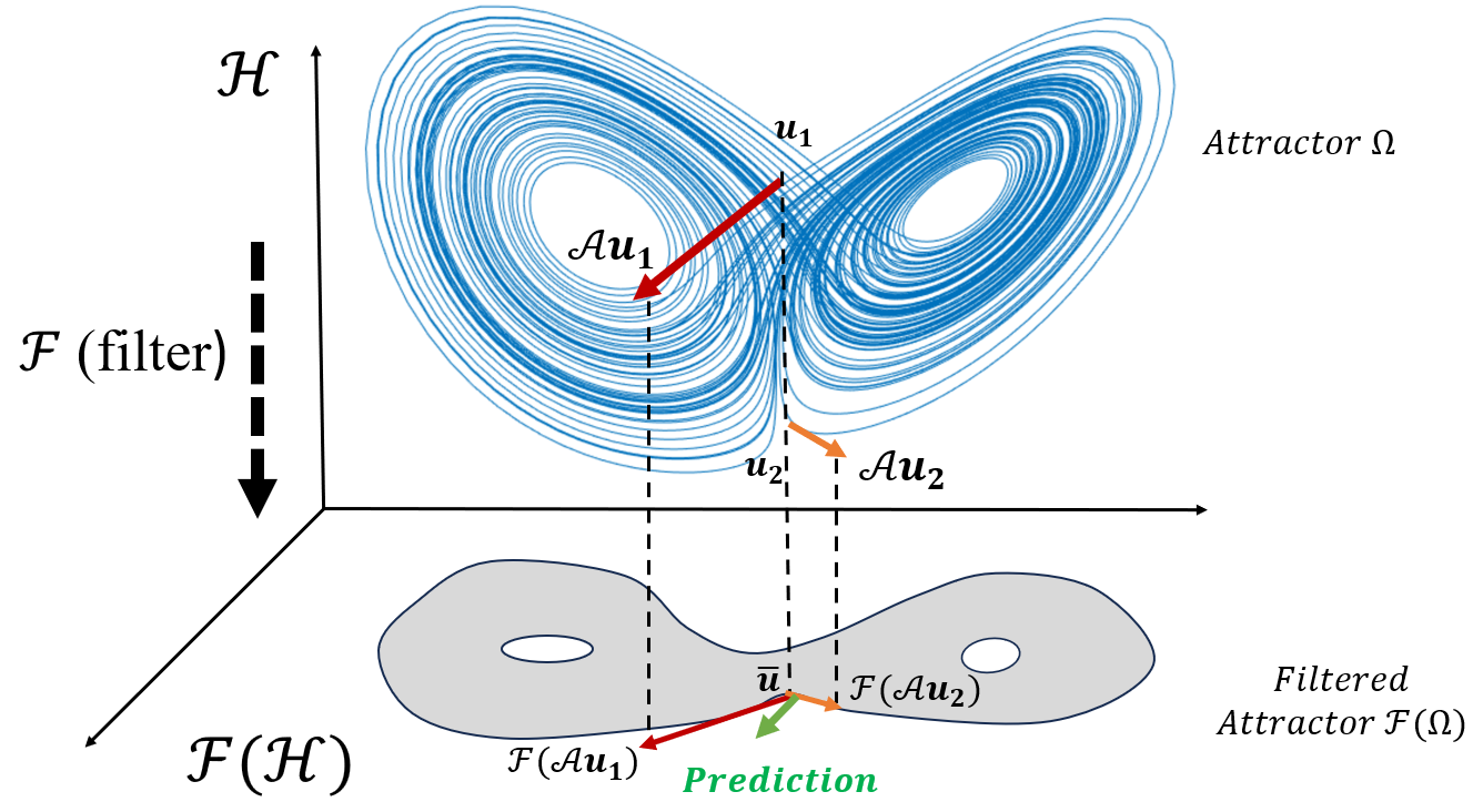
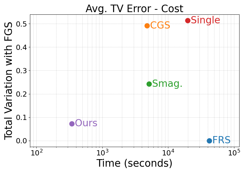
Figure 1: Left: Many points (e.g., $u_{1}$ and $u_{2}$) of the ground-truth attractor $\Omega$ (i.e., equilibrium state, blue) map to the same filtered (e.g., downsampled) value $\overline{u}$ (gray), making it impossible for the closure model to identify the correct dynamics ($\mathcal{F}(\mathcal{A}u_{1})$ and $\mathcal{F}(\mathcal{A}u_{2})$) in the filtered space $\mathcal{F}(\mathcal{H})$. By minimizing the loss function, the model learns to predict an average of these multiple choices (green arrow), which leads the simulation to wrongly diverge from the filtered attractor. Right: Total variation distance from ground-truth invariant measure versus computation cost. ‘FRS’(blue line): gold-standard fully-resolved simulations. ‘CGS’: coarse-grid simulation without closure model. ‘Smag.’: Smagorinsky model.‘Single’: learning-based single-state model. Our method is the fastest and closest to ground truth (‘FRS’) among all coarse-grid methods (‘CGS’, ‘Smag.’, ‘Single’).

Our Approach: In this work, we provide a new theoretical understanding of estimating long-term statistics of a chaotic system. We formally prove in Theorem 3.1 that for generic problems, previous learning methods based on closure models are fundamentally ill-posed since they are constrained to be on the same coarse grid as the solver, and they cannot accurately approximate the underlying chaotic system. Specifically, we prove that the mapping that closure models attempt to learn in a reduced space (coarse grid) is non-unique, i.e., there are multiple potential outputs for a given input (fig. 1, left). Hence, the standard approach to learning closure models under such non-uniqueness results in the average of possible outputs, and that cannot accurately approximate the long-term statistics of a chaotic system, no matter how large or expressive the closure model is.

We further propose an alternative end-to-end ML framework to mitigate this issue of non-uniqueness with closure models. We remove the constraint that the learned model is on a coarse grid and instead employ a grid-free approach to learning. It is based on neural operators [31, 32], which learn mappings between function spaces, as opposed to standard neural networks that are limited to a fixed grid. In a neural operator, inputs of different resolutions are viewed as different discretizations of the same function on a continuous domain, thus ensuring consistency between coarse and fine grids.

We train a neural operator model first, on data obtained from coarse-grid solvers. Since such solvers are relatively cheap to run, we can obtain sufficient data to train the neural operator to accurately emulate the coarse-grid solver. However, this is not sufficient, since our goal is to obtain the accuracy of FRS. To do this, instead of employing a separate closure model, we fine-tune the neural operator, already trained on a coarse-grid solver, using (a small amount of) FRS data and physics-based losses defined on a fine grid. Since neural operators can operate on any grid, we can employ the same model to train on data from both coarse and fine-grid solvers. The addition of physics-based losses on a fine grid further reduces the FRS data requirement and improves generalization, in line with what has been seen in prior works on physics-informed learning [33].

Table 1: Comparison between different approaches for predicting long-term statistics of Navier-Stokes equations. The Reynolds number $Re$ is large in most applications. The top two are classical approaches, and the rest are machine learning approaches. Training data is counted in the number of snapshots and trajectories. The complexity takes into account both spatial grids and temporal grids. Our approach is even cheaper than coarse-grid simulations because ours can evolve with $O(1)$ time step instead of small time-grids following the CFL condition, as is the case for other methods utilizing a coarse solver. $\delta t$ is the time-grid size for latent SDE in [34].

Method	Optimal	High-res. training data	Complexity
	statistics	FRS Snapshots | Trajs.
Fully-resolved Simulation, e.g., DNS [35, 36]	✓	-	$Re^{3.52}$
Coarse-grid Simulation, e.g., LES [35, 36]	✗	-	$Re^{2.48}$
Single-state model [30]	✗	24000 | 8	$Re^{2.48}$
History-aware model[37]	✗	250000 | 50	$Re^{2.48}$
Latent Neural SDE[34]	✗	179200 | 28	$\frac{1}{\delta t}Re^{1.86}$
Online Learning [38]	✗	-	$Re^{3.52}$
Physics-Informed Operator Learning (Ours)	✓	00110 | 1	$Re^{1.86}$

The class of neural operators has been previously established as universal approximations in function spaces [32, 39], meaning they can accurately approximate any continuous operator. We further strengthen this result here and prove in 3.1 that a neural operator that approximates the underlying ground-truth solution operator can provide sufficiently accurate estimates of the long-term statistics of a chaotic system, and there is no catastrophic build-up of errors over long rollouts. We derive all the above theoretical results through the lens of measure flow in function spaces, introducing a novel theoretical framework, viz., functional Liouville flow.

We test the performance of our approach in several instances from fluid dynamics. Our PINO model achieves 120x speedup with a relative error $\sim 5\%$ compared to FRS. In contrast, the closure model coupled with a coarse-grid solver is $58$x slower than PINO while having a much higher error $\sim 205\%$. More details about the speed-accuracy performance of different approaches are shown in figure 1.

The closure model has a significantly higher error under our setup compared to prior works [30, 29, 40]. This is because we assume that only a few FRS samples are available for training, both for PINO and the closure model, viz., just 110-time steps from a single FRS trajectory. In contrast, prior works on closure models assume thousands of time steps over hundreds of FRS trajectories. In particular, we show that to mitigate the non-unique issue of closure models mentioned above, previous methods have to resort to the closeness between the limit distribution in the original dynamics and the empirical measure of training data. Moreover, prior works assume starting the simulation close to the dynamical equilibrium of the chaotic system, whose estimation requires long rollouts of FRS, which is not realistic. Instead, we randomly initialize both PINO and closure models without any prior knowledge, and measure their performance.

An illustrative comparison between our method and representative existing methods can be found in Table 1. Our contributions are summarized as follows.

• We propose a novel framework based on functional Liouville flow, to theoretically analyze the problem of estimating long-term statistics of chaotic systems with coarse-grid simulations.

• We formally prove that restricting the learning object in the reduced space, as existing closure models do, suffers from the non-uniqueness of the learning target.

• We leverage physics-informed neural operator as an alternative approach that combines learning on data from both coarse and fine-grid solvers, and physics-based losses. We provide both theoretical and empirical evidence of its superiority.

2 Background and Existing Methods

We formally introduce the problem setting of evaluating long-term statistics as well as existing numerical and machine learning methods. We will show the potential shortcomings of previous learning methods and state some of our theoretical results. See Appendix A for more backgrounds.

2.1 Problem Background

Consider an evolution partial differential equation (PDE) that governs a (nonlinear) dynamical system in the function space,

$$\begin{cases}\partial_{t}u(x,t)=\mathcal{A}u(x,t)\\ u(x,0)=u_{0}(x),\ u_{0}\in\mathcal{H},\end{cases}$$ (1)

where $u_{0}$ is the initial value and $\mathcal{H}$ is a function space containing functions of interests, e.g., fluid field, temperature distribution, etc; see Section A.4 for further assumptions. This equation naturally induces a semigroup $\{S(t)\}_{t\geq 0}$ defined as the mapping from the initial state to the state at time $t$, $S(t):u_{0}\to u(\cdot,t)$. We refer to the set $\{S(t)u_{0}\}_{t\geq 0}$ as trajectory from $u_{0}$.

Attractor, invariant measure, long-term statistics: The (global) attractor of the dynamics is defined as the maximal invariant set of $\{S(t)\}_{t}$ towards which all trajectories converge over time. For many relevant systems, the existence of a compact attractor is either rigorously proved[41, 42] or demonstrated by extensive experiments[43, 44, 45]. The invariant measure is the time average of any trajectory, independent of initial value as long as the system is ergodic,

$$\mu^{*}:=\lim_{T\to\infty}\frac{1}{T}\int_{t=0}^{T}\delta_{S(t)u}dt,\ u\in\mathcal{H},\ a.e.$$ (2)

where $\delta$ is the Dirac measure. $\mu^{*}$ is a measure of functions and is supported on the attractor. Intuitively, the invariant measure captures the system’s long-term behavior when it reaches a dynamical equilibrium. The long-term statistics are expectations of functionals on the invariant measure. The most straightforward approach to estimate statistics is to run an accurate simulation of trajectory and compute following the definition. In practice, we first fix a sufficiently large $T$ and then choose spatiotemporal grid size accordingly so that the overall error of the simulation within $[0,T]$ remains small. We will refer to this approach as high-fidelity simulations or FRS.

Chaotic systems, characterized by positive Lyapunov exponents [46], are known for their extreme sensitivity to perturbations and catastrophic accumulation of small errors over time. To account for the unstable nature of chaotic systems, high-fidelity simulations have to be carried out on very dense spatiotemporal grids to make discretization errors small enough so that the overall error along the trajectory does not grow rapidly. This makes the FRS approach prohibitively expensive.

2.2 Coarse-grid Simulation and Closure Modeling

Given the computation cost of FRS and the fact that the ultimate goal is to evaluate the statistics instead of any individual trajectory, many works have been exploring ways to give good estimations of statistics with simulations only conducted on coarse grids. We will refer to this approach as coarse-grid simulation (CGS). It serves as the core focus of this work. Let us formalize it as follows.

Denote by $D$ the set of grid points used in FRS and $D^{\prime}$ that in CGS, with $|D^{\prime}|\ll|D|$. Simulating on $D^{\prime}$ could be viewed as evolving a filtered function $\overline{u}$ defined as $\overline{u}=\mathcal{F}u$, where $\mathcal{F}$ is a linear filtering operator. For instance, $\mathcal{F}$ is a spatial convolution for cases like down-sampling in the finite difference method and Fourier-mode truncation in the spectral method.

Theoretically, the evolution of $\overline{u}$ is governed by $\partial_{t}\overline{u}=\mathcal{F}\mathcal{A}u=\mathcal{A}\overline{u}+(\mathcal{F}\mathcal{A}-\mathcal{A}\mathcal{F})u$, where $\mathcal{F}$ and $\mathcal{A}$ are not commuting due to the nonlinearity of $\mathcal{A}$. However, the commutator $(\mathcal{F}\mathcal{A}-\mathcal{A}\mathcal{F})u$ is intractable if restricted to $D^{\prime}$ since $u$ is underresolved. To account for the effect of small scales not captured by $D^{\prime}$, in many CGS methods an adjusting term ${clos}(\overline{u};\theta)$ ($\theta$ denotes the model parameters), known as closure model, is added to the equation as a tractable surrogate model of $(\mathcal{F}\mathcal{A}-\mathcal{A}\mathcal{F})u$. The CGS trajectory is derived by simulating

$$\begin{cases}\partial_{t}{v}(x,t)=\mathcal{A}{v}(x,t)+{clos}({v};\theta),\ x\in D^{\prime}\\ {v}(x,0)=\overline{u}_{0}(x),\ \overline{u}_{0}\in\mathcal{F}(\mathcal{H}),\end{cases}$$ (3)

and the statistics are estimated as the time average of the corresponding functionals with ${v}(\cdot,t)$ input. We use the notation $v$ instead of $\overline{u}$ here to underscore the difference between coarse-grid trajectories and filtered fully-resolved trajectories, as they follow different dynamics in general.

Classical Closure Models: Closure modeling is a classical and relevant topic in computational methods for science and engineering, with rich literature available [19, 20]. Despite their wide application in numerous scenarios, the design of closure models is more of an art than science. Many existing methods are grounded in physical intuition or derived by mathematical simplifications that incorporate strong assumptions, which often do not hold up under general conditions. Additionally, selecting parameters in these closure models typically requires substantial domain expertise. Nevertheless, for several practical applications, such simple modeling assumptions are not sufficient to capture the complex optimal closure [21].

In recent years, there has been a growing interest in leveraging machine learning tools to design closure models (see [24] for survey). We summarize the mainstream methodologies as follows, along with the informal version of our theoretical results, which reveals their potential shortcomings.

Learning single-state closure model: Broadly speaking, neural network-represented closure models ${clos}(v;\theta)$ are proposed with various ansatz and neural network architectures, and they are trained by minimizing an a priori loss function aiming at fitting the commutator [24],

$$J_{ap}(\theta;\mathfrak{D})=\frac{1}{|\mathfrak{D}|}\sum\limits_{i\in\mathfrak{D}}\|clos(\overline{u}_{i};\theta)-(\mathcal{F}\mathcal{A}-\mathcal{A}\mathcal{F})u_{i}\|^{2},$$ (4)

where the training data $u_{i}$ come from snapshots of FRS trajectories, i.e., $S(t)u_{0}$ for particular $t$.

This methodology appears unconvincing when we scrutinize the input and output of the model. Due to the dimension reduction nature of filter $\mathcal{F}$, there are multiple FRS snapshots $u_{i}\in\mathcal{H}$ that end up in the same state in the reduced space $\mathcal{F}(\mathcal{H})$ (or functions restricted on $D^{\prime}$, equivalently). However, the filtering of the original vector field $\mathcal{A}u$ (describing the moving direction for the next time step), differs at these $u_{i}$. Together with the $\mathcal{A}v$ term in (3), the closure model plays the role of assigning a unique moving direction in the filtered space $\mathcal{F}(\mathcal{H})$ for each state $\overline{u}$. By minimizing the training loss (4), the model typically learns to predict the reduced vector field at $\overline{u}$ as the average (in some sense) of all these $\mathcal{F}(\mathcal{A}u_{i})$, which might not make sense. An illustration is shown in Fig. (1). To clarify, we point out the difference between our problem and many problems in inverse problems and linear regression where making an averaging prediction is logical. Model predictions need to adhere to the manifold structure characterized by physical trajectories.

There are also extensions of the learning framework above. Some works proposed to add a posterior loss into the training object [47, 48],

$$J_{post}(\theta;\mathfrak{D})=J_{ap}(\theta)+\frac{1}{|\mathfrak{D}|}\sum\limits_{i\in\mathfrak{D}}\|v_{i}(\cdot,\Delta t;\theta)-\mathcal{F}(S(\Delta t)u_{i})\|^{2},$$ (5)

where $v_{i}$ comes from evolving (3) with $\mathcal{F}u_{i}$ initialization for a time period $\Delta t$. Clearly, this modification still suffers from the issue resulting from the underdeterminancy discussed above, not to mention its heavy load of backpropagation through the numerical solver during training.

Learning history-aware closure model: As shown above, the main issue of learning a single-state closure model (i.e., the output of the closure model only depends on $\overline{u}$) is that the ‘mapping’ from $\overline{u}$ to $u$ and correspondingly $(\mathcal{F}\mathcal{A}-\mathcal{A}\mathcal{F})u$ is not a well-defined mapping, where multiple outputs are related to one single input. To handle this issue, some works [40, 37] propose to take account of history information in the reduced space, namely a closure model whose input is $\{\overline{u}(x_{i},t-s)\}_{x_{i}\in D^{\prime},\ 0<s\leq t_{0}}$ at the moment $t$, where $t_{0}$ is a model parameter.

Stochastic formulation of closure model: Another direction to handle the ill-posed issue is to replace the deterministic closure model with a stochastic one [34, 49]. This line of work is inspired by [50], which shows that the optimal choice of closure model has the form of a conditional expectation.

However, we prove that none of these approaches resolve the non-uniqueness issue. We informally summarize our results as follows.

Theorem 2.1.

(i) In general, the mapping of closure models $\overline{u}\to(\mathcal{F}\mathcal{A}-\mathcal{A}\mathcal{F})u$ is not well-defined. Consequently, the approximation error has a lower bound independent of the model complexity.
(ii) For any $u$ and finite $\tau$, there exist infinite $u^{\prime}\in\mathcal{H}$ such that $\mathcal{F}S(t)u^{\prime}=\mathcal{F}S(t)u$ for all $t\in[0,\tau)$.
(iii) One cannot obtain the best approximation of $\mu^{*}$ among distributions supported in the reduced space if there is randomness in the evolution of dynamics.

The proof can be found in Appendix C. For our second claim, since $\{\mathcal{F}S(t)u\}_{x\in D^{\prime},\ t<\tau}$ contains the entire information that could be used to predict the closure term at time $\tau$, and $\overline{u}^{\prime}(\cdot,t)$ will deviate dramatically from $\overline{u}(\cdot,t)$ in a chaotic system, the under-determinancy issue remains unsolved with history-aware models. We remark here that there have been some theoretical results stating historical information in the reduced space suffices to recover the underlying true trajectory[51], but they are all derived in ODE systems and highly rely on the finite-dimensionality of ODE systems. For our third claim, as an implication, the parameters related to randomness in the stochastic closure model will be close to zero after training. Thus, introducing randomness in the model might be redundant.

Besides the three mainstream learning-based closure modeling we loosely classified above, there are other approaches that resort to an interactive use of fine-grid simulators [52, 53] and leveraging online learning algorithms[54, 38, 23, 47]. However, calling and auto-differentiating along fully-resolved simulations make the training of this approach prohibitively expensive.

2.3 Perspective through Liouville Flow in Function Space

We have demonstrated that existing learning methods target a non-unique mapping, resulting in an average of all possible outputs, which can be undesirable. Despite this, these methods still manage to achieve competitive performance. In this section, we show that their empirical result heavily relies on the availability of a large amount of FRS training data. This dependency is a significant limitation, as FRS data are typically scarce. If a sufficient amount of FRS data were already available for training, we could directly compute the statistics using the data, eliminating the need for training a closure model or running coarse-grid simulations.

Our analysis investigates the evolution of the distribution (or measure) to determine whether it converges to $\mu^{*}$. In terms of finite-dimensional dynamical systems (ODEs), the evolution of distribution is governed by the Liouville equation. This observation motivates us to generalize the Liouville equation into function space and conduct our study therein. Rigorous definitions of related notions and detailed proofs for all claims made in this section can be found in Appendix B.

Functional Liouville Flow: If we expand functions onto an orthonormal basis, $u=\sum_{i}z_{i}\psi_{i}$, a PDE system (of $u$) can be viewed as an infinite-dimensional ODE (of ${\mathbf{z}}$). In this way, we yield the functional version of the Liouville equation describing how the probability density of $u$ evolves. Under this framework, we only need to check the stationary Liouville equation to obtain the limit invariant distribution of a dynamical system and compare it with $\mu^{*}$.

In the coarse-grid setting, we similarly derive the evolution of the density of $\overline{u}$ and yield the optimal dynamics of $v\in\mathcal{F}(\mathcal{H})$ (different from CGS in eq. 3), $v$ is exactly the same as $\overline{u}$ here),

$$\partial_{t}v=\mathbb{E}_{u\sim\mu_{t}}[\mathcal{F}\mathcal{A}u|\mathcal{F}u=v],$$ (6)

where $\mu_{t}$ is the distribution of $u\in\mathcal{H}$ following the original dynamics at time $t$ and this expectation is conditioned on the samplings of $u$ satisfying $\mathcal{F}u=v$. Here we arrive at the same result in [50]. Unfortunately, $\mu_{t}$ depends on $t$ and the initial distribution of $u\in\mathcal{H}$, which is underdetermined and will suffer from non-unique issues if restricted to a coarse-grid system, similar to what is discussed in the previous section. In practice, one can only fix one particular $\hat{\mu}$, a distribution in $\mathcal{H}$, and assign the dynamics in reduced space as $\partial_{t}v=\mathbb{E}_{u\sim\hat{\mu}}[\mathcal{F}\mathcal{A}u|\mathcal{F}u=v]$. Checking the resulting Liouville equation, we show that $\mu^{*}$ is the choice for $\hat{\mu}$ to guarantee convergence towards $\mathcal{F}_{\#}\rho^{*}$, the optimal approximation of $\mu^{*}$ in $\mathcal{F}(\mathcal{H})$. Back to the learning methods listed in Section 2.2, due to the $L^{2}$ variational characterization of conditional expectation, the underlying choice of $\hat{\mu}$ is the empirical measure of those training data coming from FRS, ideally $\mu^{*}$. Consequently, one has to use numerous FRS training data due to the slow convergence of empirical measures for high-dimensional distribution.

As is the case, these learning methods often rely on a large amount of fine-grid data coming from one long FRS trajectory or multiple FRS trajectories which are expensive. Furthermore, most methods still rely on a coarse-grid solver that iteratively evolves with relatively small time steps, and some methods require that the coarse simulation starts from a downsampled version of high-fidelity data close to the attractor. These aspects hinder the further application of these methods.

3 Methodology: Physics-Informed Operator Learning

From previous sections, we see that restricting the learning object in the filtered space and explicitly learning the closure model would always suffer from the non-uniqueness of this target. In light of that, we propose to extend the learning task into function space $\mathcal{H}$ and directly deal with the solution operator $S(t)$ of PDE governing the dynamics, which is a well-defined mapping.

Operator Learning: The goal of operator learning[31, 32, 55] is to approximate mappings between function spaces rather than vector spaces. One of the representatives is Fourier Neural Operator (FNO) [31], whose architecture can be described as:

$$\mathcal{G}_{FNO}:=\mathcal{Q}\circ({W}_{L}+\mathcal{K}_{L})\circ\cdots\circ\sigma({W}_{1}+\mathcal{K}_{1})\circ\mathcal{P},$$ (7)

where $\mathcal{P}$ and $\mathcal{Q}$ are pointwise lifting and projection operators. The intermediate layers consist of an activation function $\sigma$, pointwise operators $W_{\ell}$ and integral kernel operators $K_{\ell}:\ u\to\mathscr{F}^{-1}(R_{\ell}\cdot\mathscr{F}(u))$, where $R_{\ell}$ are weighted matrices and $\mathscr{F}$ denotes Fourier transform.

With FNO, we learn the mapping $u\to\{S(t)u\}_{t\in[0,h]}$, where $h$ is a model parameter. It has two main advantages: (1) Resolution-Invariance: The model supports input from different resolutions (grid sizes), and inputs are all viewed as discretization of an underlying function. Consequently, when we feed a coarse-grid initial state to the well-trained model and roll out to generate a CGS trajectory, there exists an FRS trajectory such that the CGS trajectory we obtain is its filtering. This CGS trajectory matches the optimal coarse-grid dynamics discussed in Section 2.3. (2) Faster Convergence: The burning time $T_{burn}$ is the moment when a trajectory approaches the attractor close enough. For previous methods, after the learning-based closure models are trained, they are merged into a coarse-grid solver and evolve iteratively with relatively small time steps. In operator learning where $h$ is usually of $O(1)$ magnitude, the simulation arrives at $T_{burn}$ more quickly.

It remains to overcome the lack of FRS training data in realistic situations. Note that the PDE(1) contains all the information of the dynamical system. We adopt physics-informed methodologies[56] to remove the reliance on data. To be specific, the operator model $\mathcal{G}_{\theta}$ is trained by minimizing the physics-informed loss function:

$$J_{pde}(\theta;\mathfrak{D})=\frac{1}{|\mathfrak{D}|}\sum_{i\in\mathfrak{D}}\|(\partial_{t}-\mathcal{A})\mathcal{G}_{\theta}u_{0i}(x)\|_{L^{2}(\Omega\times[0,h])},$$ (8)

where the initial values $u_{0i}$ in the loss function could be any fine-grid functions and do not have to come from FRS trajectories. $\Omega$ is the spatial domain of these functions.

Practical Algorithm: In practice, the optimization of physics-informed loss is hard [57] and might encounter some abnormal functions with small loss but large errors [58]. To face these challenges, we pre-train the model via supervised learning with a data loss function to achieve a good initialization of the model parameters for $J_{pde}$ optimization:

$$J_{data}(\theta;\mathfrak{D})=\frac{1}{|\mathfrak{D}|}\sum_{i\in\mathfrak{D}}\|\mathcal{G}_{\theta}u_{i}-S([0,h])u_{i}\|.$$ (9)

To enhance the limited FRS training data available, we pre-train with $J_{data}$ using plenty of CGS data first and then add FRS data into the loss function. After that, we gradually decrease the weight of CGS data loss in the loss function since CGS data is potentially incorrect. After warming up with data loss, we further train our model with physics-informed loss. The formalized algorithm and its implementation details can be found in Appendix F.

Provable Convergence to Long-term Statistics: The universal approximation capability of FNO has been proved[32, 39]. Some might doubt that since small errors will rapidly escalate over time in chaotic systems, we have to train an FNO that perfectly fits the ground truth, which would be unrealistic. However, we have the following result. Intuitively, we show that there exists a true trajectory (from a different initial value) that is consistently close to the simulation we get with approximate FNO. Since the invariant measure is independent of the initial condition, we obtain a good approximation of the (filtered) invariant measure.

Theorem 3.1.

For any $h>0$, denote $\hat{\mu}_{h,\theta}:=\lim\limits_{N\to\infty}\frac{1}{N}\sum\limits_{n=1}^{N}\delta_{\mathcal{G}_{\theta}^{n}v_{0}(x)},$ any $v_{0}(x)$ with $x\in D^{\prime}$. For any $\epsilon>0$, there exists $\delta>0$ s.t. as long as $\|(\mathcal{G}_{\theta}u)(\cdot,h)-S(h)u\|_{\mathcal{H}}<\delta,\forall u\in\mathcal{H}$, we have $\mathcal{W}_{\mathcal{H}}(\hat{\mu}_{h,\theta},\mathcal{F}_{\#}\mu^{*})<\epsilon,$ where $\mathcal{W}_{\mathcal{H}}$ is a generalization of Wasserstein distance in function space.

The proof can be found in Appendix D. Details about $\mathcal{W}_{\mathcal{H}}$ can be found in Section A.2. These results show that even if the trained operator jumps a large step $h$ in time and has errors as is in practice, we can still obtain a good estimation of statistics by rolling it out and computing the time average. In practice, a $10\%\sim 20\%$ relative error of single-step prediction suffices.

4 Experiments

We verify our algorithm with two equations from fluid dynamics, 1D Kuramoto-Sivashinsky (KS) and 2D Navier-Stokes (NS). We use one NVIDIA 4090 GPU for all experiments.

For our method, we adopt FNO as the model architecture and predict the mapping from $u_{0}$ to $\{S(t)u_{0}\}_{t\in[0,h]}$, where $h$ is of $O(1)$ magnitude. We compare our estimation of long-term statistics with gold-standard ground truth from fully resolved simulations (FRS), and several baselines. (1) CGS: coarse-grid simulation without any closure model. (2) Classical closure model: Smagorinsky model [14] is the most classical and popular closure model applied in computational fluid dynamics. We compare with Smagorinsky model for NS and its counterpart eddy-viscosity model for KS[59]. We have selected the best-performing parameter in these models. (3)  Single-state model: its methodology is showcased in Section 2.2. To leverage the up-to-date machine learning toolkits, we replace the convolution neural network (CNN) model in original papers [30] with a transformer-based model. The implementation details, hyperparameters, and data generation can be found in Appendix G and Appendix E.

(a) Energy Spectrum

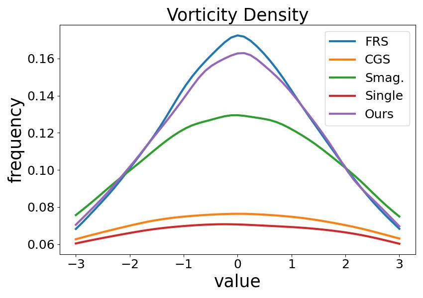
(b) Histogram of Vorticity

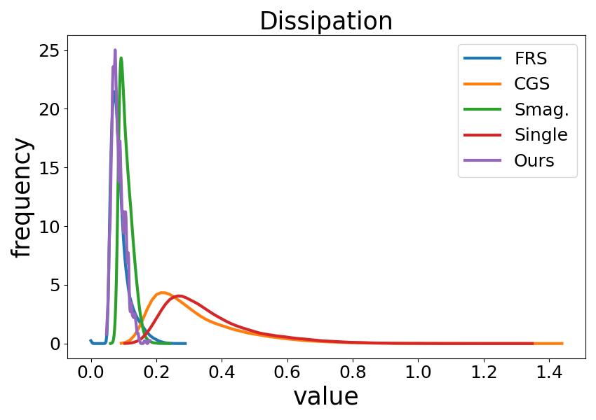
(c) Dissipation

Figure 2: Results for Navier-Stokes. (a) Energy spectrum, (b) histogram of vorticity, (c) histogram of dissipation. In the label, ‘FRS’(blue line) refers to gold-standard fully-resolved simulations. ‘CGS’: coarse-grid simulation without closure model. ‘Smag.’: Smagorinsky model. ‘Single’: single-state learning-based model. Our method is closest to ground truth (‘FRS’) among all coarse-grid methods (‘CGS’, ‘Smag.’, ‘Single’).

Kuramoto–Sivashinsky Equation We consider the one-dimensional KS equation for $u(x,t)$,

$$\partial_{t}u+u\partial_{x}u+\partial_{xx}u+\nu\partial_{xxxx}u=0,\ \ \quad(x,t)\in[0,6\pi]\times\mathbb{R}_{+},$$ (10)

with periodic boundary conditions. The positive viscosity coefficient $\nu$ reflects the traceability of this equation. The smaller $\nu$ is, the more chaotic the system is. We study the case for $\nu=0.01$.

For our model, we choose $h=0.1$. The total amount of FRS training data is 105 snapshots coming from 3 trajectories. When we complete the training, the $L^{2}$ relative error of our model on the test set is $12\%$. To make a fair comparison, other learning-based methods are restricted to the same amount of training data. This setting will be the same for NS.

Navier-Stokes Equation We consider two-dimensional Kolmogorov flow (a form of the Navier-Stokes equations) for a viscous incompressible fluid (fluid field) ${\mathbf{u}}(x,y,t)\in\mathbb{R}^{2}$,

$$\partial_{t}{\mathbf{u}}=-({\mathbf{u}}\cdot\nabla){\mathbf{u}}-\nabla p+\frac{1}{Re}\Delta{\mathbf{u}}+(\sin(4y),0)^{T},\quad\nabla\cdot{\mathbf{u}}=0,\quad(x,y,t)\in[0,2\pi]^{2}\times\mathbb{R}_{+},$$ (11)

with periodic boundary conditions. The function $p$ is a known pressure. The positive coefficient $Re$ is Reynolds number. The larger $Re$ is, the more chaotic the system is. We consider the case $Re=100$.

For our model, we choose $h=1$. The total amount of FRS training data is 110 snapshots coming from 1 trajectory. When we complete the training, the $L^{2}$ relative error on the test set is $19\%$.

Table 2: Experiment Results for Navier-Stokes Equation. Left: Errors on different statistics, i.e., average total variation (‘Avg. TV’), energy spectrum (‘Energy’), TV error for vorticity distribution (‘Vorticity’), and velocity variance (‘Variance’). Percentages refer to average relative errors. Other numbers refer to TV distances (ranging $[0,1]$) between ground truth and prediction. Right: Comparison of the inference time (seconds) of one trajectory for $t\in[0,100]$. Best results are marked bold.

Method	Avg. TV	Energy	Vorticity	Variance
CGS (No closure)	0.4914	178.4651%	0.1512	253.4234%
Smagorinsky [14]	0.2423	52.9511%	0.0483	20.1740%
Single-state [30]	0.5137	205.3709%	0.1648	298.2027%
Our Method	0.0726	5.3276%	0.0091	2.8666%

FRS	39.70
CGS (No closure)	4.50
Smagorinsky	4.81
Single-state	18.57
Ours	0.32

Evaluation: Inspired by Section 2.3 where we analyze through the viewpoint of probability distributions, we propose to compare the predicted invariant measure and ground truth directly, in that we can get a good estimation of any statistics as long as we estimate the distribution well. To be specific, we compute the total variation (TV) distance between marginal distributions of every $z_{i}$ component(Section 2.3). To give a more convincing comparison, we also check useful statistics like energy spectrum, auto-correlation, variance, velocity and vorticity density, kinetic energy and dissipation rate. Due to the space limit, a comprehensive comparison of error and visualization of these statistics, along with their definitions, are presented in Appendix G. We also refer the readers to the appendix for details on how we compute the statistics and results for the KS equation.

For NS equation, we average over 400 trajectories from $t\in[1800,3000]$ to compute the statistics. The error of some statistics (compared with FRS) and the running time of a single trajectory for $t\in[0,100]$ are shown in Table 2. Visualization for the prediction of these three statistics is shown in Figure 2. A cost-error (in terms of average total variation distance from ground-truth invariant measure for among all $z_{i}$) summary is presented in fig. 1 right.

From the result, we see that even though using a very limited number of FRS training data, our method manages to estimate long-term statistics accurately and efficiently, much better than all the baselines. We also see that previous learning-based methods perform quite badly when restricted to a realistic usage of FRS data, much worse than reported in original papers where they use thousands of data or hundreds of trajectories for training.

An ablation study to demonstrate the effect of data-loss pretraining is carried out in section G.3.

5 Conclusions

In this work, we study the problem of estimating long-term statistics in chaotic systems with only coarse-grid simulations. We propose a new theoretical framework, functional Liouville flow, to analyze this problem. We rigorously demonstrate the inherent shortcomings of existing learning methods. Also inspired by our theoretical result, we leverage physics-informed neural operators to give an efficient and provably accurate estimation of long-term statistics with very limited fine-resolution data usage during training. As evaluated in the experiments, our method has the potential to address the challenging tasks regarding chaotic systems arising in various physical sciences. The implication of this work is not restricted to the specific task of estimating long-term statistics. This work exhibits the benefit of going beyond the finite grid system and understanding problems through a function space viewpoint. Functional Liouville flow would be useful in investigating image generation tasks, by viewing images as functions represented on pixels.

Acknowledgements

A. Anandkumar is supported in part by Bren endowed chair, ONR (MURI grant N00014-18-12624), and by the AI2050 senior fellow program at Schmidt Sciences. J. Berner acknowledges support from the Wally Baer and Jeri Weiss Postdoctoral Fellowship. C. Wang hopes to thank Andrew Stuart, Ricardo Baptista, and Arushi Gupta for helpful discussions.

Appendix

In this appendix, we will first provide detailed proofs of our theoretical results (A-D), and then present implementation details and more experiment results (E-G). The structure of the appendix is as follows.

• Appendix A provides a list of notations, along with an introduction of important background conceptions, preliminary results, and basic assumptions in this paper.

• Appendix B first formally introduces functional Liouville flow, and then presents a detailed version of Section 2.3.

• Appendix C provides the proof of the three claims in 2.1.

• Appendix D provides the proof of 3.1.

• Appendix E contains information about the dataset in the experiments and a visualization of the Navier-Stokes dataset.

• Appendix F provides the implementation details for our method and baseline methods.

• Appendix G first formally introduces the statistics we consider, followed by the full experiment results (table and plots) and ablation studies.

Appendix A Notations, Auxiliary Results, and Basic Assumptions

In this section, we first summarize the notations in this paper, then review and define some of the important concepts, and finally state the basic assumptions in this work. We would encourage the readers to always check this section when they have any confusion regarding the proof.

A.1 Notations

Table 3: List of Notations

Notation	Description
$\mu$	Distributions.
$F_{\#}$	Push-forward of a mapping $F$. If $y=F(x)$ and the distribution of $x$ is $\mu_{x}$, then the distribution of $y$ is $F_{\#}\mu_{x}$.
$F^{\#}$	Pull-back of a mapping $F$. If $y=F(x)$ and the distribution of $y$ is $\mu_{y}$, then the distribution of $x$ is $F^{\#}\mu_{y}$.
$\mathcal{H}$	(Original) Function Space, see eq. 1.
$\mathcal{A}$	The operator of the dynamics, see eq. 1.
$S(t)$	Semigroup induced by eq. 1.
$u$	Functions in $\mathcal{H}$.
$\mathcal{F}$	Filter. $\mathcal{F}:\mathcal{H}\to\mathcal{H}$. The image space is finite-rank and denoted as $\mathcal{F}(\mathcal{H})$.
$D$	The set of grids in fully-resolved simulations. The number of grids is $|D|$.
$D^{\prime}$	The set of grids in coarse-grid simulations. The number of grids is $|D^{\prime}|$.
$\mathscr{P}(\Omega)$	The set of all probability distributions supported on a set $\Omega$.
$\mathcal{W}_{\mathcal{H}}$	The Wasserstein distance for measures in $\mathcal{H}$, with $\|\cdot\|_{\mathcal{H}}$ being the cost function.
$\langle\cdot,\cdot\rangle$	The pair of linear functionals and elements in a Banach space $\mathscr{X}$. Specifically, for $x\in\mathscr{X},\ f\in\mathscr{X}^{*}$, its dual space, $\langle f,x\rangle:=f(x)$. Thanks to Riesz Representation Theorem, we will also use this notation for inner products in Hilbert space.
$\otimes$	For a Hilbert space $\mathcal{H}$, $u\in\mathcal{H}$, $v\in\mathcal{H}$, $u\otimes v$ is defined as the linear operator $w\to\langle v,w\rangle u,\ w\in\mathcal{H}$.
$\oplus$	$u\oplus v:=(u,v)$.
$C_{0}$	Continuous function space, equipped with $L^{\infty}$ norm.
$C_{c}^{\infty}$	Smooth and compactly-supported functions.
$d\mathcal{G}(u,v)$	The Gateaux derivative of operator $\mathcal{G}$ at $u$ in the direction of $v$.
$\aleph_{0}$	Aleph-zero, countably infinite.
$[n]$	$\{1,2,...n\}$
$D_{T}$	The set of time-grids.
$M_{D_{T}}(u_{0})$	The set of functions that are indistinguishable from $u_{0}$ merely based on values on spatiotemporal grid $D^{\prime}\times D_{T}$, see C.5.
$I_{x},\ I$	(Spatial) Grid-measurement operators, see C.1.
$\mathfrak{F}_{D_{T}},\ \mathfrak{F}$	Spatiotemporal grid-measurement operators, see C.2.
$w.r.t.$	with regard to
$wlog$	without loss of generality

A.2 Optimal Transport in Function Space

Given a Banach space $\mathscr{X}$ and two distributions $\mu_{1},\mu_{2}\in\mathscr{P}(\mathscr{X})$, we want to measure the closeness of these two distributions.

Recall that in finite-dimensional $\mathscr{X}$, the (Monge formulation of) $c-Wasserstein$ distance is defined as

$$\mathcal{W}_{c}(\mu_{1},\mu_{2}):=\inf_{T}\int_{\mathscr{X}}c(x,Tx)\mu_{1}(dx),\quad s.t.\ T_{\#}\mu_{1}=\mu_{2},$$ (12)

where $T$ is a measurable mapping from $\mathscr{X}$ to $\mathscr{X}$, and $c=c(x,y)$ is non-negative bi-variate function known as cost function.

We could naturally generalize this concept into measures in arbitrary Banach space $\mathscr{X}$ and define the Wasserstein distance correspondingly. In particular, we use the metric in $\mathscr{X}$ as cost function and define

$$\mathcal{W}_{\mathscr{X}}(\mu_{1},\mu_{2}):=\inf_{T}\int_{\mathscr{X}}\|Tx-x\|\mu_{1}(dx),\quad s.t.\ T_{\#}\mu_{1}=\mu_{2}.$$ (13)

For more backgrounds and rigorous definitions of concepts appeared above, [60, 61] are standard references for optimal transport, and [62, 63] are good references for measure theory (and probability) in function space.

A.3 Dynamical Systems

We would like to refer the readers to classical textbooks on dynamical systems [64, 65] and ergodic theorems [66] for detailed proofs of lemmas stated in this subsection.

A.3.1 Discrete Time System

Let $X$ be a compact metric space and $f:X\to X$ be a continuous map. The generic form of discrete-time dynamical system is written as $x_{n+1}=f(x_{n}),\ n\in\mathbb{N}$ or $n\in\mathbb{Z}$ (if $f$ is a homeomorphism).

Definition A.1.

$\Lambda\subsetneqq X$ is an invariant set of $f$ if $f(\Lambda)=\Lambda$.

In the following discussion, we further assume $X$ to be a $C^{\infty}$ Riemannian manifold without boundary.

Definition A.2.

An invariant set $\Lambda\subsetneqq X$ of $f$ is hyperbolic if for each $x\in\Lambda$, the tangent space $T_{x}X$ splits into a direct sum

$$T_{x}X=E^{s}(x)\oplus E^{u}(x),$$ (14)

invariant in the sense that

$$Tf(E^{s}(x))=E^{s}(f(x)),\ Tf(E^{u}(x))=E^{u}(f(x)),$$ (15)

such that, for some constant $C\geq 1$ and $\lambda\in(0,1)$, the following uniform estimates hold:

$$|Tf^{n}(v)|\leq C\lambda^{n}|v|,\ \forall x\in\Lambda,\ v\in E^{s}(x),\ n\geq 0,$$ (16)

$$|Tf^{n}(v)|\geq\frac{1}{C}\lambda^{-n}|v|,\ \forall x\in\Lambda,\ v\in E^{u}(x),\ n\geq 0.$$ (17)

Lemma A.3.

(Shadowing Lemma) Let $\Lambda\subset X$ be a hyperbolic set of $f$. For any $\epsilon>0$, there is $\eta_{0},\eta_{1}>0$ such that for any $\{x_{n}\}_{n\in\mathbb{N}}$ satisfying (i) $d(x_{n},\Lambda)<\eta_{0}$; (ii) $|x_{n+1}-f(x_{n})|<\eta_{1}$ for all $n$, there exists $y\in X$ such that $|x_{n}-f^{(n)}y|<\epsilon,\ \forall n.$

A.3.2 Continuous Time System

Recall that the dynamical system we consider is

$$\begin{cases}\partial_{t}u(x,t)=\mathcal{A}u(x,t)\\ u(x,0)=u_{0}(x),\ u_{0}\in\mathcal{H},\end{cases}$$ (18)

where $u_{0}$ is the initial value and $\mathcal{H}$ is a function space containing functions of interests. We will occasionally refer to $\mathcal{A}u$ as vector field governing the dynamics. This dynamics induced a semigroup $\{S(t)\}_{t\geq 0}$.

Definition A.4.

Given a measure $\mu\in\mathscr{P}(\mathcal{H})$, the system is mixing if for any measurable set $A,\ B\subset\mathcal{H}$, $\lim\limits_{t\to\infty}\mu(A\cap S(t)(B))=\mu(A)\mu(B).$

Definition A.5.

A measure $\mu\in\mathscr{P}(\mathcal{H})$ is said to be an invariant measure of this system if $S(t)_{\#}\mu=\mu$ for all $t>0.$

Lemma A.6.

If a system is mixing, then it is ergodic.

For ergodic systems, there is an invariant measure independent of the initial condition, defined as

$$\mu^{*}:=\lim_{T\to\infty}\frac{1}{T}\int_{t=0}^{T}\delta_{S(t)u}dt,\ u\in\mathcal{H},\ a.e.$$ (19)

where $\delta$ is the Dirac measure.

Definition A.7.

The semigroup is said to be uniformly compact for t large, if for every bounded set $B\subset\mathcal{H}$ there exists $t_{0}$ which may depend on $B$ such that $\cup_{t\geq t_{0}}S(t)B$ is relatively compact in $\mathcal{H}$.

Lemma A.8.

If S(t) is uniformly compact, then there is a compact attractor in this system.

A.4 Assumptions

Without loss of generality, we carry out our discussion in the regime where $\mathcal{H}$ is a separable Hilbert space to make the proof more readable and concise. We also make the following technical assumptions.

Assumption A.9.

$\mathcal{H}$ can be compactly embedded into $C_{0}$.

Assumption A.10.

The system eq. 18 is mixing. The semigroup is uniformly compact.

Assumption A.11.

The attractor and invariant measure are unique.

Assumption A.12.

The attractor is hyperbolic w.r.t $S(t)$ for any $t>0$.

We remark that these assumptions are either proved or supported by experimental evidence in many real scenarios [67, 68, 43, 69].

For brevity, we will ignore the difference between fully-resolved simulation (FRS) and the exact solution to eq. 18 in the following discussions.

Appendix B Formal Introduction of Functional Liouville Flow

In this section, we first formally introduce functional Liouville flow in Section B.1. Based on this theoretical framework, we will reformulate the task of estimating long-term statistics of dynamical systems with coarse-grid simulations in Section B.2. Finally, we will provide in Section B.3 a detailed version of the discussion in Section 2.3.

B.1 Framework of Functional Liouville Flow for studying Invariant Measure

Functions as vectors:

As a corollary of Hahn-Banach theorem, we could always construct a set of orthonormal basis $\{\psi_{i}\}_{i}$ of $\mathcal{H}$ such that the filtered space $\mathcal{F}(\mathcal{H})=\mathrm{span}\{\psi_{1},...\psi_{n}\}$, where we usually have $n=|D^{\prime}|$. For any function $u\in\mathcal{H}$, there exists a unique decomposition $u(x)=\sum_{i=1}^{\infty}z_{i}\psi_{i}(x)$ with $z_{i}=\langle u,\psi_{i}\rangle$. This canonically induces an isometric isomorphism:

$$\mathcal{T}:\ \mathcal{H}\to\ell^{2},\quad u\mapsto{\mathbf{z}}=(z_{1},z_{2},...).$$ (20)

By this means, we can rewrite the original PDE(18) into an ODE in $\ell^{2}$, denoted by

$$\frac{d{\mathbf{z}}}{dt}=f({\mathbf{z}}),\ \mathrm{where}\ f({\mathbf{z}})\in\ell^{2},\ f({\mathbf{z}})_{i}=\langle\psi_{i},\mathcal{A}\circ\mathcal{T}^{-1}{\mathbf{z}}\rangle,$$ (21)

where $\langle,\rangle$ is the inner product in $\mathcal{H}$.

Example B.1.

For Kuramoto–Sivashinsky Equation

$$\partial_{t}u+u\partial_{x}u+\partial_{xx}u+\partial_{xxxx}u=0,\ \ \quad(x,t)\in[0,2\pi]\times\mathbb{R}_{+},$$ (22)

if we choose $\{\psi_{k}\}$ as the Fourier basis $\{e^{ikx}\}_{k\in\mathbb{Z}}$, then $z_{k}$ is the coefficient of $k$-th Fourier mode and the ODE for ${\mathbf{z}}$ is (component-wise),

$$\frac{dz_{k}}{dt}=(-k^{4}+k^{2})z_{k}-\frac{ik}{2}\sum_{j+l=k}z_{j}z_{l}.$$ (23)

One could further make $z_{k}$ real numbers by choosing $\sin,\ \cos$ basis.

Functional Liouville flow:

Recall that in ODE system $\frac{dx}{dt}=f(x),\ x\in\mathbb{R}^{d}$, if the initial state $x_{0}$ follows the distribution $\mu_{0}$ whose probability density is $\rho_{0}(x)$, then the probability density of $x(t)$, denoted by $\rho(x,t)$, satisfies the Liouville equation,

$$\partial_{t}\rho=-\nabla\cdot(f\rho).$$ (24)

Now we want to generalize this result into function space. We need to address the issue that there is in general no probability density function for measures in function space. We will show that it is reasonable to carry on our study by fixing a sufficiently large $N$ and investigating the truncated system of the first $N$ basis, and viewing the densities as the (weak-)limit when $N\to\infty$.

Proposition B.2.

For any $\mu$ supported on a bounded set $B\subset\mathcal{H}$ and any $\epsilon>0$, there exsits $t_{0}$ and $N$ s.t. for any $u_{0}\sim\mu$ and any $t>t_{0}$, if we write $S(t)u_{0}$ as $\sum_{i=0}^{\infty}z_{i}\psi_{i}$, then $\|\sum_{i>N}z_{i}\psi_{i}\|<\epsilon$.

Proof.

Define $Q_{m}:=\sum_{i>m}\psi_{i}\otimes\psi_{i}$. Then the statement is equivalent to $\|Q_{N}S(t)u_{0}\|<\epsilon,\$for all $u\in B,t>t_{0}.$

Due to A.10, there exists $t_{0}$ such that $\cup_{t>t_{0}}S(t)B$ is relatively compact. This implies that there exists finite (denoted by $N_{1}$) points $\{u_{i}\}$ satisfying that for any $u_{0}\in B,\ t>t_{0}$, there exists $i\leq N_{1}$ s.t. $\|S(t)u_{0}-u_{i}\|<\frac{\epsilon}{3}$. We define $M_{i}:=\min_{j}\{j|\|Q_{j}u_{i}\|<\frac{\epsilon}{5}\}$. We have $M_{i}<\infty,\ \forall i.$ Choosing $N$ as $\max\limits_{i\leq N_{1}}M_{i}$ completes the proof. ∎

Remark B.3.

We can always restrict our discussion within distributions supported on bounded set whose complement occurs with a probability smaller than machine precision.

Back to the dynamics eq. 18 or the equivalent ODE eq. 21, we first make a generalization. Since the invariant measure is independent of initial condition, we know that for any distribution $\mu_{0}\in\mathscr{P}(\mathcal{H})$(instead of only delta distributions at $u_{0}$) from which we sample random initial conditions $u_{0}\sim\mu_{0}$ and evolve these functions, the long-term average $\lim\limits_{T\to\infty}\frac{1}{T}\int_{t=0}^{T}\big{(}S(t)_{\#}\big{)}\mu_{0}dt$ will still converge to $\mu^{*}$. We will carry out our discussion in this generalized setting where the initial condition is sampled from a distribution $\mu_{0}$ in function space. We will denoted $\big{(}S(t)_{\#}\big{)}\mu_{0}$, the distribution at time $t$, as $\mu_{t}$, and denoted their density functions for corresponding ${\mathbf{z}}$ as $\rho(\cdot,t)$ (i.e., $\mu_{t}=\mathcal{T}^{\#}\rho(\cdot,t)$). For brevity, we will view $u\in\mathcal{H}$ and ${\mathbf{z}}\in\ell^{2}$ as the same and not mention $\mathcal{T}^{\#}$ or $\mathcal{T}_{\#}$ for $\mu_{t}$ and $\rho(\cdot,t)$.

If we use the component-form of $f$, $f=(f_{1},f_{2},....)$, with each $f_{i}$ a mapping from $\ell^{2}\to\mathbb{R}$, with exactly the same argument to derive eq. 24, we have

$$\partial_{t}\rho({\mathbf{z}},t)=-\sum_{i}^{\infty}\partial_{z_{i}}(f_{i}({\mathbf{z}})\rho({\mathbf{z}},t)):=-\nabla_{{\mathbf{z}}}\cdot(f\rho),\qquad\rho({\mathbf{z}},0)=\rho_{0}({\mathbf{z}}).$$ (25)

We will refer to this as functional Liouville flow, i.e., the Liouville equation in function space, and denote the R.H.S. operator $\rho\to-\nabla_{{\mathbf{z}}}\cdot(f\rho)$ as $\mathscr{L}\rho$.

Reinterpretation of Invariant Measure:

With functional Liouville flow, we obtain a new characterization of invariant measure $\mu^{*}$ (whose distribution is denoted as $\rho^{*}$).

Proposition B.4.

$\rho^{*}$ is the solution to stationary Liouville equation $\mathscr{L}\rho=0$.

Proof.

Denote $p({\mathbf{z}},t):=\frac{1}{t}\int_{s=0}^{t}\rho({\mathbf{z}},s)ds$, the finite-time average distribution.

Note that for any ${\mathbf{z}}$,

$$\rho({\mathbf{z}},t)= \rho({\mathbf{z}},0)+\int_{s=0}^{t}\partial_{t}\rho({\mathbf{z}},s)ds$$ (26)

$$= \int_{0}^{t}\mathscr{L}\rho({\mathbf{z}},s)ds+\rho({\mathbf{z}},0)$$ (27)

$$= \mathscr{L}\int_{s=0}^{t}\rho(z,s)ds+\rho({\mathbf{z}},0)=\mathscr{L}(tp({\mathbf{z}},t))+\rho({\mathbf{z}},0).$$ (28)

Also, we have $\rho({\mathbf{z}},t)=\partial_{t}(\int_{s=0}^{t}\rho({\mathbf{z}},s)ds)=\partial_{t}(tp({\mathbf{z}},t))$, we conclude that

$$\partial_{t}(tp({\mathbf{z}},t))=t\mathscr{L}p({\mathbf{z}},t)+\rho({\mathbf{z}},0).$$ (29)

From this, we yield

$$\partial_{t}p({\mathbf{z}},t)=\mathscr{L}p({\mathbf{z}},t)+\frac{1}{t}(\rho({\mathbf{z}},0)-p({\mathbf{z}},t)).$$ (30)

By definition we know $p({\mathbf{z}},t)\to\rho^{*}$ as $t\to\infty$, thus $\partial_{t}p\to 0$. The term $\frac{1}{t}(\rho({\mathbf{z}},0)-p({\mathbf{z}},t))$ will also tend to zero as $t\to\infty$ (recall that they are probability density and thus are uniformly bounded in $L^{1}$). Therefore, the limit density $\rho^{*}$ satisfies $\mathscr{L}\rho^{*}=0$. ∎

B.2 Reformulation of Estimating Long-term Statistics

We reformulate the problem of estimating long-term statistics with coarse-grid simulation with the help of functional Liouville flow. Recall that $D^{\prime}$ is the set of coarse grid points, and coarse-grid simulation (CGS) is equivalent to evolving functions in $\mathcal{F}(\mathcal{H})$, where $\mathcal{F}$ is the filter (see Section 2.2).

B.2.1 Notations

We start by defining several notations.

Define the orthonormal projection onto $\mathcal{F}(\mathcal{H})$ as ${P}=\sum\limits_{i=1}^{n}\psi_{i}\otimes\psi_{i}$. We remark here that in many situations, we have $P=\mathcal{F}$.

Let us decomposite ${\mathbf{z}}$ and $u$ into the resolved part and unresolved part,

$${\mathbf{z}} ={\mathbf{v}}\oplus{\mathbf{w}},\ {\mathbf{v}}:=(c_{1},c_{2},...c_{n}),\ {\mathbf{w}}:=(c_{n+1},c_{n+2},...);$$ (31)

$$u(x) =v(x)+w(x),\ v(x):=\mathcal{T}^{-1}{\mathbf{v}}=Pu,\ w(x):=\mathcal{T}^{-1}{\mathbf{w}}=(I-P)u.$$ (32)

In particular, $w\in\mathcal{F}(\mathcal{H})^{\perp}$ is the unresolved part in coarse-grid simulations. With this decomposition, we rewrite any density $\rho({\mathbf{z}})$ as a joint distribution $\rho({\mathbf{v}},{\mathbf{w}})$ and define marginal distribution for ${\mathbf{v}}$ as $\rho_{1}({\mathbf{v}})$, and the conditional distribution of ${\mathbf{w}}$ given ${\mathbf{v}}$ as $\rho({\mathbf{w}}|{\mathbf{v}})$. With a little abuse of notation, we will occasionally refer to the probability density as its distribution, and vice versa.

We will also divide the vector field $f$ into resolved part $f_{r}$ and unresolved part $f_{u}$, which are $(f_{1},f_{2},...,f_{n})$ and $(f_{n+1},f_{n+2},...)$ respectively.

B.2.2 Reformualtion of Coarse-grid Simulation

We first show that the optimal approximation of $\mu^{*}$ (or $\rho^{*}$) in the reduced space is its marginal distribution, if we construct densities with orthonormal basis, as is in eq. 20.

Proposition B.5.

$\rho_{1}^{*}=\operatorname*{arg\,min}\limits_{\mu\in\mathscr{P}(\mathcal{F}(\mathcal{H}))}\mathcal{W}_{\mathcal{H}}(\mu,\mu^{*})$.

Proof.

From the construction of $P$ and the definition of $\mathcal{W}_{\mathcal{H}}$, for any measurable mapping
$\mathfrak{T}:\mathcal{H}\to\mathcal{F}(\mathcal{H})$,

$$\int_{\mathcal{H}}\|\mathfrak{T}u-u\|\mu^{*}(du)\geq\int_{\mathcal{H}}\|Pu-u\|\mu^{*}(du).$$ (33)

Thus, for any $\mu\in\mathscr{P}(\mathcal{F}(\mathcal{H}))$,

$$\mathcal{W}_{\mathcal{H}}(\mu,\mu^{*})\geq\int_{\mathcal{H}}\|Pu-u\|\mu^{*}(du)=\mathcal{W}_{\mathcal{H}}(P_{\#}\mu^{*},\mu^{*}).$$ (34)

Note that $\rho_{1}^{*}=P_{\#}\mu^{*}$, this completes the proof. ∎

This result motivates us to check the evolution of $\rho_{1}({\mathbf{v}},t)$, which should achieve the optimal approximation $\rho^{*}_{1}$.

Note that by definition, for any distribution $\rho\in\mathscr{P}(\mathcal{H})$, $\rho_{1}({\mathbf{v}})=\int\rho({\mathbf{v}},{\mathbf{w}})d{\mathbf{w}}$. Combine this with eq. 25, we yield

$$\partial_{t}\rho_{1}({\mathbf{v}},t)= \int\partial_{t}\rho({\mathbf{v}},{\mathbf{w}},t)d{\mathbf{w}}$$ (35)

$$= -\int\nabla_{{\mathbf{v}}}\cdot(f_{r}({\mathbf{v}},{\mathbf{w}})\rho({\mathbf{v}},{\mathbf{w}},t))d{\mathbf{w}}-\int\nabla_{{\mathbf{w}}}\cdot(f_{u}({\mathbf{v}},{\mathbf{w}})\rho({\mathbf{v}},{\mathbf{w}},t))d{\mathbf{w}}$$ (36)

$$= -\nabla_{\mathbf{v}}\cdot\bigg{(}\frac{\rho_{1}({\mathbf{v}},t)}{\rho_{1}({\mathbf{v}},t)}\int f_{r}({\mathbf{v}},{\mathbf{w}})\rho({\mathbf{v}},{\mathbf{w}},t)d{\mathbf{w}}\bigg{)}-0$$ (37)

$$= -\nabla_{\mathbf{v}}\cdot\bigg{(}\rho_{1}({\mathbf{v}},t)\int f_{r}({\mathbf{v}},{\mathbf{w}})\frac{\rho({\mathbf{v}},{\mathbf{w}},t)}{\int\rho({\mathbf{v}},{\mathbf{w}}^{\prime},t)d{\mathbf{w}}^{\prime}}d{\mathbf{w}}\bigg{)}$$ (38)

$$= -\nabla_{\mathbf{v}}\cdot\big{(}\rho_{1}({\mathbf{v}},t)\mathbb{E}_{{\mathbf{w}}\sim\rho({\mathbf{w}}|{\mathbf{v}};t)}[f_{r}({\mathbf{v}},{\mathbf{w}})|{\mathbf{v}}]\big{)}.$$ (39)

where we use the divergence theorem for the second term in the second line.

The corresponding ODE dynamics for this Liouville equation eq. 39 is

$$\frac{d{\mathbf{v}}}{dt}=\mathbb{E}_{{\mathbf{w}}\sim\rho({\mathbf{w}}|{\mathbf{v}};t)}[f_{r}({\mathbf{v}},{\mathbf{w}})|{\mathbf{v}}].$$ (40)

If we transform it back into $\mathcal{H}$ space, it becomes (informally)

$$\partial_{t}v=\mathbb{E}_{u\sim\mu_{t}}[\mathcal{F}\mathcal{A}u|\mathcal{F}u=v],$$ (41)

as is presented in Section 2.3 in main text. This describes (one of) the optimal dynamics in the reduced space.

B.2.3 The Effect of Closure Modeling

Apart from the original motivation of closure modeling to approximate the commutator $\mathcal{F}\mathcal{A}-\mathcal{A}\mathcal{F}$, we alternatively interpret it as assigning a vector field $\mathcal{A}_{\theta}$ in the reduced space $\mathcal{F}(\mathcal{H})$ and accordingly the coarse-grid dynamics is

$$\partial_{t}v=\mathcal{A}_{\theta}v,$$ (42)

here $\mathcal{A}_{\theta}$ plays the role of $\mathcal{A}v+clos(v;\theta)$ in eq. 3.

We will refer to both $\mathcal{A}_{\theta}$ and $clos(\cdot;\theta)$ as the target of closure modeling for brevity.

As an application of Proposition B.4, we only need to check the solution to the stationary Liouville equation related to this dynamics to decide whether or not the resulting limit distribution is the optimal one $\rho_{1}^{*}$.

B.3 Detailes for Discussion in Section 2.3

The dynamics of the filtered trajectory in Equation 41 (we will refer to the equivalent version eq. 40 for convenience), which is also derived in [50], has inspired many works for the design of closure models. Unfortunately, we want to point out that it is impractical to utilize this result for closure model design.

The decision regarding subsequent motion at the state $({\mathbf{v}},t)$ have to made only based on information from the reduced space, which contains merely ${\mathbf{v}}$ itself and the distribution of ${\mathbf{v}}$. For any given ${\mathbf{v}}$, only one prediction can be made for the next time step. Similar to the non-uniqueness issue highlighted in Section 2, however, since $\rho({\mathbf{w}}|{\mathbf{v}};t)$ depends on $t$ and $\rho_{0}$(the initial distribution of $u\in\mathcal{H}$), typically there are multiple distinct $\rho({\mathbf{v}},{\mathbf{w}},t)$ with exactly the same ${\mathbf{v}}$ and marginal distribution in $\mathcal{F}(\mathcal{H})$.

In practice, if one hopes to follow the form of conditional expectation as in eq. 40, he can only fix one particular $q({\mathbf{v}},{\mathbf{w}})$, a distribution in $\mathcal{H}$, and assign the vector field in reduced space as $\mathbb{E}_{{\mathbf{w}}\sim q({\mathbf{w}}|{\mathbf{v}})}[f_{r}({\mathbf{v}},{\mathbf{w}})\big{|}{\mathbf{v}}]$.

Now, we check the limit distribution we will obtain with this dynamics. From Proposition B.4, we know that limit distribution $\hat{\rho}_{1}({\mathbf{v}})$ is the solution to (usually in weak sense)

$$\nabla_{\mathbf{v}}\cdot\bigg{(}\mathbb{E}_{{\mathbf{w}}\sim q({\mathbf{w}}|{\mathbf{v}})}[f_{r}({\mathbf{v}},{\mathbf{w}})\big{|}{\mathbf{v}}]\rho_{1}({\mathbf{v}})\bigg{)}=0.$$ (43)

Proposition B.6.

$\rho_{1}^{*}$ is the solution to eq. 43 if $q=\rho^{*}$.

Proof.

By definition, $\rho^{*}({\mathbf{v}},{\mathbf{w}})$ satisfies

$$\nabla_{{\mathbf{v}}}\cdot(f_{r}({\mathbf{v}},{\mathbf{w}})\rho^{*}({\mathbf{v}},{\mathbf{w}},t))+\nabla_{{\mathbf{w}}}\cdot(f_{u}({\mathbf{v}},{\mathbf{w}})\rho^{*}({\mathbf{v}},{\mathbf{w}},t))=0.$$ (44)

Integral over ${\mathbf{w}}$ and use divergence theorem, we yield

$$0 =\int\nabla_{\mathbf{v}}\cdot\big{(}f_{r}({\mathbf{v}},{\mathbf{w}})\rho^{*}({\mathbf{v}},{\mathbf{w}})\big{)}d{\mathbf{w}}+0$$ (45)

$$=\nabla_{\mathbf{v}}\cdot\int f_{r}({\mathbf{v}},{\mathbf{w}})\rho_{1}^{*}({\mathbf{v}})\rho^{*}({\mathbf{w}}|{\mathbf{v}})d{\mathbf{w}}$$ (46)

$$=\nabla_{\mathbf{v}}\cdot\bigg{(}\mathbb{E}_{{\mathbf{w}}\sim\rho^{*}({\mathbf{w}}|{\mathbf{v}})}[f_{r}({\mathbf{v}},{\mathbf{w}})\big{|}{\mathbf{v}}]\rho_{1}({\mathbf{v}})\bigg{)}$$ (47)

This gives the proof. ∎

Thus, we show that $\rho^{*}$ is the correct choice for $q$ to guarantee convergence towards $\rho_{1}^{*}$ in $\mathcal{F}(\mathcal{H})$. Back to the learning methods discussed in Section 2.2, if we follow the new interpretation in Section B.2.3, the loss function is

$$J_{ap}(\theta) =\mathbb{E}_{u\sim p_{data}}\|\mathcal{A}_{\theta}\mathcal{F}u-\mathcal{F}\mathcal{A}u\|^{2}$$ (48)

$$=\mathbb{E}_{({\mathbf{v}},{\mathbf{w}})\sim p_{data}({\mathbf{v}},{\mathbf{w}})}|f_{r}({\mathbf{v}};\theta)-f_{r}({\mathbf{v}},{\mathbf{w}})|^{2},$$ (49)

where we transform the original objective function into $\ell^{2}$ space of ${\mathbf{z}}$ in the second line, and $f_{r}(\cdot;\theta)$ is the counterpart of $\mathcal{A}_{\theta}$ in $\ell^{2}$, $p_{data}$ is the empirical measure of training data from fully-resolved simulations(FRS).

Due to the $L^{2}$ variational characterization of conditional expectation, the underlying choice of $q({\mathbf{v}},{\mathbf{w}})$ in those existing learning methods is ${p}_{data}$. Consequently, one has to use numerous FRS training data due to the slow convergence of empirical measure of the high-dimensional distribution $\rho^{*}$.

Appendix C Proof of Theorem 2.1

For the first claim in 2.1, it has already been shown in the main text that the mapping of closure model $\overline{u}\to(\mathcal{F}\mathcal{A}-\mathcal{A}\mathcal{F})u$ is not well-defined. We will make this claim more precise in Section C.1, and then give the proof for the second claim in Section C.2 and the proof for the third claim in Section C.3.

C.1 Proof of 2.1(i)

By transforming the original dynamics into the space of $\ell^{2}$, it is easier to see why the mapping of closure model is not well-defined. Since $\mathcal{A}\mathcal{F}u=\mathcal{A}\overline{u}$, we only need to show that $\overline{u}\to\mathcal{F}\mathcal{A}u$ is not well defined. The counterpart of this mapping in $\ell^{2}$ space is ${\mathbf{v}}\to f_{r}({\mathbf{v}},{\mathbf{w}})$. If it were a well-defined mapping, there would be a mapping $\tilde{f}_{r}({\mathbf{v}})$ such that $f_{r}({\mathbf{v}},{\mathbf{w}})\equiv\tilde{f}_{r}({\mathbf{v}})$ for all ${\mathbf{w}}$. In other words, the reduced system is independent of the unresolved part. This property rarely holds in most dynamical systems, except for a few trivial cases like the heat equation.

Next we show that the approximation error has a positive lower bound.

We could always construct $u_{1},u_{2}\in\mathcal{H}$ such that $\overline{u}_{1}=\overline{u}_{2}$ and $\mathcal{F}\mathcal{A}u_{1}\neq\mathcal{F}\mathcal{A}u_{2}$. Therefore, for any model $clos(\overline{u};\theta)$ the approximation error

$$\sup_{u\in\mathcal{H}}\|clos(\overline{u};\theta)-(\mathcal{F}\mathcal{A}-\mathcal{A}\mathcal{F})u\|_{\mathcal{H}}$$ (50)

$$\geq \sup_{u\in\{u_{1},u_{2}\}}\|clos(\overline{u};\theta)-(\mathcal{F}\mathcal{A}-\mathcal{A}\mathcal{F})u\|_{\mathcal{H}}$$ (51)

$$\geq \frac{1}{2}\big{(}||(\mathcal{F}\mathcal{A}-\mathcal{A}\mathcal{F})u_{1}-clos(\overline{u};\theta)||_{\mathcal{H}}+||clos(\overline{u};\theta)-(\mathcal{F}\mathcal{A}-\mathcal{A}\mathcal{F})u_{2}||_{\mathcal{H}}\big{)}$$ (52)

$$\geq \frac{1}{2}||(\mathcal{F}\mathcal{A}-\mathcal{A}\mathcal{F})u_{1}-(\mathcal{F}\mathcal{A}-\mathcal{A}\mathcal{F})u_{2}||_{\mathcal{H}}$$ (53)

$$= \frac{1}{2}\|\mathcal{F}(\mathcal{A}u_{1}-\mathcal{A}u_{2})\|_{\mathcal{H}}$$ (54)

has a lower bound independent of the model, where we apply the fact that $\mathcal{F}u_{1}=\mathcal{F}u_{2}=\overline{u}$ in the last line.

C.2 Proof of Theorem 2.1(ii)

Notations: Recall that $\mathcal{H}$ is the function space, and $D^{\prime}$ is the set of coarse grid points,
$D^{\prime}=\{x_{1},x_{2},...,x_{n}\}$. The filtered value of two functions being the same is equivalent to the fact that these two functions have the same values on the grid points in $D^{\prime}$.

Definition C.1.

Define grid-measurement operator (at $x_{0}$)

$$I_{x_{0}}:\ \mathcal{H}\to\mathbb{R}:\ u\mapsto u(x_{0})$$ (55)

For brevity, we will use $I_{j}$ for $I_{x_{j}}$. We further define $I_{D^{\prime}}$ (abbreviated as $I$ if there is no ambiguity),

$$I_{D^{\prime}}:\ \mathcal{H}\to\mathbb{R}^{n},\ u\mapsto(u(x_{1}),u(x_{2}),...u(x_{n}))^{T}.$$ (56)

Before we delve into the details of the proof, we would like to remind the readers of heat equation as an concrete and easy-to-check example where our result holds.

Our original theorem is stated for a continuous time interval. We first prove its finite version.

Theorem C.2.

Given $D_{T}$ the set of time grids, with $|D_{T}|=N$ and $D_{T}=\{t_{1},t_{2},...t_{N}\}$, for any $r\in\mathbb{N}$, any function $u_{0}\in\mathcal{H}\cap C_{0}$, there exists an $r$-dimensional manifold $M_{r}\subset\mathcal{H}\cap C_{0}$ such that

$$IS(t)u^{\prime}=IS(t)u_{0},\ \forall t\in D_{T},\ \forall u^{\prime}\in M_{r}.$$ (57)

Proof.

For $m\in\mathbb{N}$, given $m$ linearly independent functions $\{\phi_{i}\}_{1\leq i\leq m}\subset\mathcal{H}$, we can construct an affine manifold $A:=u_{0}+\operatorname{span}\{\phi_{1},...\phi_{m}\}$ and define the following mapping (spatiotemporal grid-measurement operator):

$$\mathfrak{F}=\mathfrak{F}_{D_{T}}:\ A\to\mathbb{R}^{nN}$$ (58)

$$v\ \mapsto\ \mathop{\bigoplus_{j=1}^{N}}IS(t_{j})v.$$ (59)

Note that we have a canonical coordinate system for $A$:

$$\ A\ \leftrightarrow\mathbb{R}^{m}$$ (60)

$$v=u_{0}+\sum_{i=1}^{m}c_{i}\phi_{i}\ \leftrightarrow(c_{1},...c_{m}),$$ (61)

thus, $\mathfrak{F}$ is a mapping between finite-dimensional manifolds, and we can compute its Jacobian
$\mathcal{J}(v)\in\mathbb{R}^{m\times Nn}$, whose elements consist of the grid-measurement of Gateaux derivatives, $I_{j}dS(t_{k})(v,\phi_{l}),\ j\in[n],\ k\in[N],\ l\in[m]$.

By a generalization of Sard’s theorem for Banach manifold [70], we know that for any $u_{0}$, any $r$, there exists $m=Nn+r$ linearly independent functions $\{\phi_{i}\}_{i=1}^{m}$ such that the Jacobian is everywhere full-rank (i.e., rank$=Nn$) in the affine manifold $A$. By pre-image theorem, since $\mathfrak{F}^{-1}\{\mathfrak{F}u_{0}\}$ is non-empty (for at least $\mathfrak{F}u_{0}$ is in this set), it is an $m-Nn=r$ dimensional manifold. This gives the proof. ∎

Corollary C.3.

Given $D_{T}$ the set of time grids, with $|D_{T}|=N$ and $D_{T}=\{t_{1},t_{2},...t_{N}\}$, for any $r\in\mathbb{N}$, any function $u_{0}\in\mathcal{H}\cap C_{0}$, there exists infinite $u^{\prime}\in\mathcal{H}$ such that $IS(t)u^{\prime}=IS(t)u_{0}$ for all $t\in D_{T}$.

Proof.

For any $r\geq 1$, there are infinite points in the manifold we yield in the theorem above. ∎

Remark C.4.

We require $u\in C_{0}$ only to exclude the artificial case of modifying the function value on a zero-measure set.

From the result above, we see that for any $u_{0}$ and finite time-grid set $D_{T}$, $\mathfrak{F}^{-1}\{\mathfrak{F}u_{0}\}$ is an infinite-dimensional manifold. To complete our proof, we make two technical assumptions. One can check these assumptions for specific dynamical systems to derive the final result. We also remark that they are not the weakest set of assumptions to guarantee the final result, we adopt them here primarily to keep the proof concise.

For a time-grid set $D_{T}$, and a function $u_{0}$, we denote as $M_{D_{T}}(u_{0})$ the set of all functions $u^{\prime}$ that $IS(t)u^{\prime}=IS(t)u_{0},\ \forall t\in D_{T}$.

Assumption C.5.

For every $u_{0}$ and finite $D_{T}$, the infinite-dimensional manifold $M_{D_{T}}(u_{0})$ is unbounded.

Assumption C.6.

Given any finite $\tau$, and an arbitrary bounded set $\Omega\subset\mathcal{H}$, we could assign a sequence of linearly independent functions $\{\phi_{i;u}\}_{i=1}^{\infty}\subset\mathcal{H}$ for each $u\in\mathcal{H}$ such that for any functions $u,\ v$, any subset $B\subset\mathbb{N}$, and any finite subset $D_{T}$ of $[0,\tau]$, there exists a continuous mapping

$$G:\ M_{D_{T}}(u)\bigcap\big{\{}u+\operatorname{span}\{\phi_{i;u}\mid i\in B\}\big{\}}\to M_{D_{T}}(v)\bigcap\big{\{}v+\operatorname{span}\{\phi_{i;v}\mid i\in B\}\big{\}}$$ (62)

depending only on $u,\ v,\ B,\ D_{T}$, such that

$$\sup\limits_{w\in\Omega\cap M_{D_{T}}(u)}\|Gw-w\|\leq C_{\Omega}\|u-v\|,$$ (63)

where the constant $C_{\Omega}$ only depends on $\Omega$ and $\tau$, and not on $u,\ v,\ B,\ D_{T}$.

Before moving on, we first review a classical result.

Lemma C.7.

There exists a bijection between $\mathbb{N}$ and $\mathbb{N}^{2}$.

Proof.

This is a standard result in set theory, and its proof can be found in many textbooks.

We give an example on how to construct such a bijection (see Figure 3). We write 1,2,3,4,… zigzaggingly to fill the $\mathbb{N}^{2}$ plane. In this way, we construct a mapping $\iota:\mathbb{N}^{2}\to\mathbb{N}$, with $\iota(i,j)$ defined as the value written at $(i,j)$-position in the $\mathbb{N}^{2}$ plane. Clearly, $\iota$ is a bijection. ∎

With $\iota$, we can partition $\mathbb{N}$ into $\aleph_{0}$(countably infinite) disjoint subsequences, $\{\iota(i,j)\}_{j\in\mathbb{N}}$ for each $i$.

Figure 3: Illustration of a bijection between $\mathbb{N}$ and $\mathbb{N}^{2}$ using a zigzag numbering scheme.

We are finally ready for the proof of 2.1(ii).

Theorem C.8.

For any $u\in\mathcal{H}$ and finite $\tau$, there exist infinite $u^{\prime}\in\mathcal{H}$ such that $\mathcal{F}S(t)u^{\prime}=\mathcal{F}S(t)u$ for all $t\in[0,\tau)$.

Proof.

Let $\mathcal{K}$ be a dense Hilbert subspace of $\mathcal{H}$ that can compactly embedded into $\mathcal{H}$, with norm $\|\cdot\|_{\mathcal{K}}$. For instance, if $\mathcal{H}=H^{k}$, the Sobolev space $W^{2,k}$, then we can choose $\mathcal{K}$ as $H^{k+1}$.

Step 1: We first deal with the case when $u\in\mathcal{K}$.

Define a sequence of time-grid set $D_{j}$ as $\{\frac{i}{2^{j}}\tau|0\leq i<2^{j}\}$. Similar to the argument in C.2, we can construct a sequence $\{\phi_{i}\}_{i=1}^{\infty}\subset\mathcal{K}$ satisfying the following properties.

1. They are linearly independent.

2. For any $j\in\mathbb{N}$, $m>2^{j}$, $B\subset\mathbb{N}$ with $|B|=m$, the spatiotemporal grid-measurement $\mathfrak{F}$ for $D^{\prime}\times D_{j}$ has full-rank Jacobian everywhere in the affine manifold $u+\operatorname{span}\{\phi_{k}:\ k\in B\}.$

Based on the $\mathbb{N}-\mathbb{N}^{2}$ bijection $\iota$, we define the following subspaces:

$$E_{k}:=\operatorname{span}\{\phi_{\iota(k,i)}:\ i\in\mathbb{N}\}.$$ (64)

There are $\aleph_{0}$ such subspaces in total, we will next find a point $u^{\prime}$ in each $E_{k}$ such that
$IS(t)u^{\prime}=IS(t)u$ for all $t\in[0,\tau)$.

WLOG, we will only show how to construct $u^{\prime}$ in $E_{1}$.

We denote

$$M_{j}=E_{1}\cap M_{D_{j}}(u).$$ (65)

By the construction of $D_{j}$ we have $M_{1}\supset M_{2}\supset M_{3}\supset...$.

We first fix three constants $0<B_{0}<B_{1},\ B_{2}>0$ and and construct a sequence of $\{u_{i}\}\subset E_{1}$ such that

1. $u_{i}\in M_{i}$.

2. $B_{0}<\|u_{i}-u\|_{\mathcal{H}}<B_{1}$.

3. $\|u_{i}\|_{\mathcal{K}}<B_{2}$.

This construction is achievable due to C.5 and the fact that $u\in\mathcal{K}$.

Since $\mathcal{K}$ can be compactly embedded into $\mathcal{H}$, there there exists a subsequence $\{u_{i_{j}}\}$ of $\{u_{i}\}$ that is convergent in $\mathcal{H}$. We denote its limit as $u_{\infty}$. From (ii), we have $\|u_{\infty}\|_{\mathcal{H}}<\infty$ and $u_{\infty}\neq u$.

Due to A.9, we have $u_{i_{j}}\to u_{\infty}$ in $C_{0}$, which implies that for any $D_{j}$, $\mathfrak{F}_{D_{j}}u_{\infty}=\mathfrak{F}_{D_{j}}u$.

Because of the continuity of the mapping $t\mapsto I_{x}S(t)v$ for any $x\in D^{\prime},\ v\in\mathcal{H}$, we know that $IS(t)u^{\prime}=IS(t)u$ for all $t\in[0,\tau)$.

To conclude, for each $E_{k}$, there exists $u^{\prime}\in E_{k}$ that is not distinguishable from $u$ merely based on function values restricted to the grid $D^{\prime}\times D_{T}$. Recall that for any $j\neq k$, by construction we have $E_{j}\cap E_{k}=\{u\}$, thus these $u^{\prime}$ in different $E_{k}$ are mutually different. This completes the proof for the case $u\in\mathcal{K}$.

Step 2 Now we give the proof for general $u\in\mathcal{H}$.

Since $\mathcal{K}$ is dense in $\mathcal{H}$, there exists a sequence $\{u^{n}\}\subset\mathcal{K}$ such that $\|u^{n}-u\|_{\mathcal{H}}<\frac{1}{2^{n}}$. We keep using the constant $B_{0},B_{1},B_{2}$ and define $\Omega:=\{v\in\mathcal{H}\mid\|v-u\|_{\mathcal{H}}<B_{1}+1\}$. Following C.6, we obtain the constant $C_{\Omega}$ and linearly independent set $\{\phi_{i;u^{n}}\}_{i=1}^{\infty}$ for each $n$. Following the first part of this proof, we define

$$E_{k}^{n}:=\operatorname{span}\{\phi_{\iota(k,i);u^{n}}\mid i\in\mathbb{N}\}\quad M_{j,k}^{n}:=E_{k}^{n}\cap M_{D_{j}}(u^{n}),$$ (66)

and again we only need to consider the case when $k=1$, and thus abbreviate $M_{j,k}^{n}$ as $M_{j}^{n}$.

We will restrict our discussion within $n>n_{0}:=\bigg{\lceil}\max\{\log_{2}\frac{6(C_{\Omega}+1)}{B_{0}},\log_{2}3(C_{\Omega}+1)\}\bigg{\rceil}+1$.

We inductively construct a sequence (indexed by $n$) of sequence $\{u_{j}^{n}\}_{j}\subset E_{1}^{n}$ as follows:

(I) For $n=n_{0}$, we construct $\{u^{n}_{j}\}_{j}$ the same as the first part of the proof.

1. $u_{j}^{n}\in M_{j}^{n}$.

2. $B_{0}<\|u_{j}^{n}-u^{n}\|_{\mathcal{H}}<B_{1}$.

3. $\|u_{j}^{n}\|_{\mathcal{K}}<B_{2}$.

(II) Now suppose we have constructed $\{u^{n}_{j}\}_{j}$, we apply C.6 for $u^{n},\ u^{n+1}$,
$B=\{\iota(1,i)\mid i\in\mathbb{N}\}$ and $D_{j}$ and obtain a continuous mapping $G$. We choose $u^{n+1}_{j}$ as $Gu_{j}^{n}$.

Next, we give some estimations for $u_{j}^{n+1}$.

First, note that we have

$$\|u^{n}-u^{n+1}\|_{\mathcal{H}}\leq\|u^{n}-u\|_{\mathcal{H}}+\|u-u^{n+1}\|_{\mathcal{H}}<\frac{3}{2^{n+1}},$$ (67)

and thus $\|u_{j}^{n}-u_{j}^{n+1}\|_{\mathcal{H}}\leq C_{\Omega}\frac{3}{2^{n+1}}$ by construction. Based on this, we have

$$\|u_{j}^{n+1}-u^{n+1}\|_{\mathcal{H}} \geq\|u_{j}^{n}-u^{n}\|_{\mathcal{H}}-\|u_{j}^{n}-u_{j}^{n+1}\|_{\mathcal{H}}-\|u^{n}-u^{n+1}\|_{\mathcal{H}}$$ (68)

$$\geq\|u_{j}^{n}-u^{n}\|_{\mathcal{H}}-\frac{3(C_{\Omega}+1)}{2^{n+1}}.$$ (69)

By induction, we have

$$\|u_{j}^{n+1}-u^{n+1}\|_{\mathcal{H}}\geq\|u_{j}^{n_{0}}-u^{n_{0}}\|_{\mathcal{H}}-\sum_{n>n_{0}}\frac{3(C_{\Omega}+1)}{2^{n+1}}>\frac{B_{0}}{2}.$$ (70)

We also have

$$\|u_{j}^{n+1}-u^{n+1}\|_{\mathcal{H}} \leq\|u_{j}^{n}-u^{n}\|_{\mathcal{H}}+\|u_{j}^{n}-u_{j}^{n+1}\|_{\mathcal{H}}+\|u^{n}-u^{n+1}\|_{\mathcal{H}}$$ (71)

$$\leq\|u_{j}^{n}-u^{n}\|_{\mathcal{H}}+\frac{3(C_{\Omega}+1)}{2^{n+1}}.$$ (72)

By induction, we have

$$\|u_{j}^{n+1}-u^{n+1}\|_{\mathcal{H}}\leq\|u_{j}^{n_{0}}-u^{n_{0}}\|_{\mathcal{H}}+\sum_{n>n_{0}}\frac{3(C_{\Omega}+1)}{2^{n+1}}<B_{1}+\frac{1}{2}.$$ (73)

Similar to what is done in the first part of the proof, we can choose $v^{n_{0}}$ as one of the limit points of $\{u^{n_{0}}_{j}\}_{j}$. Inductively, we can construct a sequence of $v^{n}$ such that

1. $v^{n}$ is one of the limit points of $\{u^{n}_{j}\}_{j}$

2. $\|v^{n}-v^{n-1}\|_{\mathcal{H}}\leq\frac{3C_{\Omega}+1}{2^{n}}$.

Thus, $\{v^{n}\}_{n}$ is a Cauchy sequence in $\mathcal{H}$ and we denote its limit as $v$. Because of A.9, we have that $IS(t)v=IS(t)u,\ \forall t\in[0,\tau)$. It is also clear that

$$v\in M_{[0,\tau)}(u)\cap\big{\{}u+\operatorname{span}\{\phi_{\iota(1,i);u}\mid i\in\mathbb{N}\}\big{\}},$$ (74)

and

$$\|v-u\|_{\mathcal{H}}=\|\lim\limits_{n\to\infty}(v^{n}-u^{n})\|_{\mathcal{H}}\geq\liminf_{n\to\infty}\|u^{n}-v^{n}\|_{\mathcal{H}}\geq\frac{B_{0}}{2}.$$ (75)

With exactly the same argument as in the first step, we construct infinite mutually-different functions that are not distinguishable from $u$ on $D^{\prime}\times[0,\tau)$. This completes the proof. ∎

C.3 Proof of Theorem 2.1(iii)

Theorem C.9.

One cannot obtain the $\rho_{1}^{*}$ if there is randomness in the evolution of dynamics.

Proof.

Our proof will be carried out for a more general setting.

Consider two dynamics

$$\frac{d{\mathbf{v}}}{dt}=b_{1}({\mathbf{v}})$$ (76)

$$d{\mathbf{v}}=b_{2}({\mathbf{v}})dt+\sigma({\mathbf{v}})dW.$$ (77)

The first one corresponds to the deterministic motion as is in the original dynamical system (transformed into $\ell^{2}$). Either $\rho^{*}$ it $\rho^{*}_{1}$ is the limit distribution of certain deterministic dynamics. The second one corresponds to the dynamics of the stochastic closure model. Here $dW$ is a $d$ dimensional Brownian motion where $d$ is the latent dimension of the model.

From Appendix B, we know that the limit distribution of eq. 76 is the solution to stationary Liouville equation,

$$\nabla\cdot(b_{1}\rho)=0.$$ (78)

As for eq. 77, similar to how we handle deterministic systems in Appendix B and how we derive the Fokker-Planck equation in finite-dimensional systems, we can generalize Fokker-Planck equation into function space and yield that the limit distribution of eq. 77 is the solution to stationary Fokker-Planck equation,

$$\nabla\cdot(b_{2}\rho)-\frac{1}{2}\nabla^{2}:(\sigma\sigma^{T}\rho)=0.$$ (79)

Next, we argue by contradiction to show that $\rho_{1}^{*}$ or $\rho^{*}$ will not satisfy eq. 79.

Suppose $\rho_{1}^{*}$ is the solution to both eq. 78 and eq. 79. We then have that for any $k\in\mathbb{R}$, $\rho_{1}^{*}$ is the solution to

$$\nabla\cdot(kb_{1}+b_{2}\rho)-\frac{1}{2}\nabla^{2}:(\sigma\sigma^{T}\rho)=0.$$ (80)

We can expand this equation and write it in the following form

$$A({\mathbf{v}}):\nabla^{2}\rho+B_{k}({\mathbf{v}})\cdot\nabla\rho+C_{k}({\mathbf{v}})\rho=0,$$ (81)

in particular, $A=-\frac{1}{2}\sigma\sigma^{T}$ and $C_{k}({\mathbf{v}})$ has the form $C({\mathbf{v}})+k\nabla\cdot b_{1}$.

Recall that $\rho_{1}^{*}$ is supported on the compact attractor(denoted as $\Omega$) of the original dynamical system. Now let us consider the maximum point of $\rho_{1}^{*}$ in $\Omega$. If there exists local maximum point ${\mathbf{v}}_{0}\in\Omega^{\circ}$(its interior), then the Hessian of $\rho^{*}_{1}$ at ${\mathbf{v}}_{0}$ is semi-negative-definite and $\nabla\rho_{1}^{*}({\mathbf{v}}_{0})=0$. Thus we have

$$C_{k}({\mathbf{v}}_{0})\rho_{1}^{*}({\mathbf{v}}_{0})=-A({\mathbf{v}}):\nabla^{2}\rho_{1}^{*}({\mathbf{v}}_{0})\geq 0.$$ (82)

We could always choose $k$ such that the L.H.S. has a negative value. Contradiction!

This suggests that there is no local maxima of $\rho^{*}_{1}$ in $\Omega^{\circ}$. Thus, the maxima of $\rho^{*}_{1}$ is on the boundary. However, $\rho_{1}^{*}\big{|}_{\partial\Omega}=0$. This suggests $\rho_{1}^{*}=0$. Contradiction!

This completes the proof.

∎

Appendix D Proof of Theorem3.1

As a preliminary result, we show the following properties of the dynamical systems under consideration.

Lemma D.1.

For any $h>0$, any initial condition $u_{0}\in\mathcal{H}$, $\lim\limits_{N\to\infty}\frac{1}{N}\sum\limits_{n=1}^{N}\delta_{S(nh)u_{0}}=\mu^{*}.$

Proof.

Denote $G:=S(h)$. From A.10, we know that for any measurable set $A,\ B\subset\mathcal{H}$, $\lim\limits_{t\to\infty}\mu(A\cap S(t)(B))=\mu(A)\mu(B).$ In particular $\lim\limits_{n\to\infty}\mu(A\cap S(nh)(B))=\mu(A)\mu(B).$ This suggests that the system defined by

$$u_{n+1}=Gu_{n}$$ (83)

is mixing.

From Lemma A.6, this system is ergodic, thus having an invariant measure w.r.t $G$. Since $G_{\#}\mu^{*}=\mu^{*}$, due to the uniqueness of invariant measure, we derive the proof. ∎

In the following proof, we will use the notation $G:=S(h)$, which is the learning target (ground-truth operator), and $\hat{G}$ for the approximate operator we obtain after training. By the design of the neural operator, the input of $\hat{G}$ can be vectors in $\mathbb{R}^{d}$ for any dimensionality $d$, serving as various discretizations of a particular function from $\mathcal{H}$. Here we violate the concepts a little bit by denoting $\hat{G}$ as a mapping from $\mathcal{H}$ to $\mathcal{H}$ (approximating $S(h)$) instead of $\mathcal{H}$ to $\mathcal{H}\times[0,h]$(approximating $u\to\{S(t)u\}_{t\leq h}$) as is in our algorithm in main. In practice, we only use the last element of the output sequence, corresponding to the prediction for $S(h)u$, for estimating statistics. To be specific, to estimate long-term statistics in coarse-grid systems with learned operator $\hat{G}$, we use as input a function in reduced space $v(x)\in\mathcal{F}(\mathcal{H}),\ x\in D^{\prime}$ (equivalent to an $\mathbb{R}^{|D^{\prime}|}$ vector consisting of the function values on the grids), and autoregressively compute $\hat{G}^{(n)}v,\ n\in\mathbb{N}$. The invariant measure is estimated by

$$\hat{\mu}_{D^{\prime}}:=\lim\limits_{N\to\infty}\frac{1}{N}\sum_{n=1}^{N}\delta_{\hat{G}^{(}n)v}.$$ (84)

We first remind readers of the following fact.

Fact D.2.

For any function $u_{0}\in\mathcal{H}$, let $\vec{u}:=(u_{0}(x_{1}),...u_{0}(x_{n}))^{T},\ n=|D^{\prime}|$, be the discretization of $u_{0}$ in the coarse-grid system. There exists $u\in\mathcal{H}$ (possibly different from $u_{0}$) such that

$$\vec{u}=I_{D^{\prime}}u^{\prime},\quad\hat{G}(\vec{u})=I_{D^{\prime}}\hat{G}u.$$ (85)

Now, we prove our main result.

Theorem D.3.

For any $h>0$ and any $\epsilon>0$, there exists $\delta>0$ such that, as long as
$\|\hat{G}u-Gu\|_{\mathcal{H}}<\delta,\ \forall u\in\mathcal{H}$, we will have $\mathcal{W}_{\mathcal{H}}(\hat{\mu}_{D^{\prime}},\rho_{1}^{*})<\epsilon$.

Proof.

We will first deal with dynamics in the original space $\mathcal{H}$. We have two dynamics, the exact one and the approximate one,

$$u^{n+1} =Gu^{n},\ u^{0}=u_{0}\in\mathcal{H};$$ (86)

$$\hat{u}^{n+1} =\hat{G}\hat{u}^{n},\ \hat{u}^{0}=u_{0}\in\mathcal{H}.$$ (87)

Both dynamics will converge to an attractor, $\Omega$ and $\hat{\Omega}$, respectively.

With Lemma A.3, we know that there exists $\eta_{0},\eta_{1}>0$ such that for any $\{u_{n}\}_{n\in\mathbb{N}}\subset\mathcal{H}$ satisfying
(i) $d(u_{n},\Omega)<\eta_{0}$; (ii) $\|u_{n+1}-G(u_{n})\|<\eta_{1}$ for all $n$, there exists $\tilde{u}\in\mathcal{H}$ such that

$$\|u_{n}-G^{(n)}\tilde{u}\|<\epsilon,\ \forall n\in\mathbb{N}.$$ (88)

From Therorem 1.2 in Chapter 1 of [67], we know that there exists $\eta_{2}>0$ such that

$$\|Gu-\hat{G}u\|<\eta_{2},\ \forall u\in\mathcal{H}\Rightarrow\ dist(\Omega,\hat{\Omega})<\frac{\eta_{0}}{5}.$$ (89)

Now we choose $\delta$ as $\min\{\eta_{1},\eta_{2}\}$ and define the approximate operator $\hat{G}$ as well as dynamics and attractor accordingly.

We next choose $n_{0}\in\mathbb{N}$ such that $\sup_{n\geq n_{0}}dist(\hat{u}^{n},\hat{\Omega})<\frac{\eta_{0}}{5}$. This implies that $\sup_{n\geq n_{0}}dist(\hat{u}^{n},{\Omega})<\frac{3\eta_{0}}{5}$. We apply Lemma A.3 to obtain a function $\tilde{u}\in\mathcal{H}$ such that

$$\|u^{n}-G^{(n-n_{0})}\tilde{u}\|<\epsilon,\ \forall n\geq n_{0}.$$ (90)

For any $N\in\mathbb{N}$, we define

$${\mu}_{N}: =\frac{1}{N}\sum_{n=0}^{N}\delta_{G^{(n)}\tilde{u}}$$ (91)

$$\hat{\mu}_{N}: =\frac{1}{N}\sum_{n=n_{0}}^{n_{0}+N}\delta_{\hat{u}^{n}}.$$ (92)

By constructing the transport mapping $T:u^{n}\mapsto G^{(n-n_{0})}\tilde{u},\ n_{0}\leq n\leq n_{0}+N$, we have that

$$\mathcal{W}_{\mathcal{H}}(\hat{\mu}_{N},\mu_{N})<\epsilon.$$ (93)

Note that $\hat{\mu}_{N}\to\hat{\mu}_{D}$(estimated invariant measure with fine-grid simulations) as $N\to\infty$, we derive

$$\mathcal{W}_{\mathcal{H}}(\hat{\mu}_{D},\mu^{*})\leq\epsilon.$$ (94)

Recall that $P$ is the orthonormal projection towards $\mathcal{F}(\mathcal{H})$ and that $\|Pu-Pu^{\prime}\|\leq\|u-u^{\prime}\|$ for any $u,u^{\prime}\in\mathcal{H}$. In light of D.2, we derive $\mathcal{W}_{\mathcal{H}}(\hat{\mu}_{D^{\prime}},\rho_{1}^{*})\leq\epsilon$. ∎

Appendix E Experiment Setup and Data Generation

E.1 Kuramoto–Sivashinsky Equation

We consider the following one-dimensional KS equation for $u(x,t)$,

$$\partial_{t}u+u\partial_{x}u+\partial_{xx}u+\nu\partial_{xxxx}u=0,\ \ \quad(x,t)\in[0,L]\times\mathbb{R}_{+},$$ (95)

with periodic boundary conditions. The positive viscosity coefficient $\nu$ reflects the traceability of this equation. The smaller $\nu$ is, the more chaotic the system is. We study the case for $\nu=0.01,\ L=6\pi$.

FRS is conducted with exponential time difference 4-order Runge-Kutta (ETDRK4)[71] with 1024 uniform spatial grid and $10^{-4}$ time grid. The CGS is conducted with the same algorithm except with 128 uniform spatial grids and $10^{-3}$ timegrid. We choose $h=0.1$ for our model.

Dataset

The training dataset for the neural operator consists of two parts, the CGS data and FRS data. The CGS dataset contains 6000 snapshots from 100 CGS trajectories. Snapshots are collected from time $t=20+k$, $k=1,2....60$. The data appears as input-label pairs $(v(\cdot,t),v(\cdot,t+h))$, where $h=0.1$ for KS. The FRS dataset contains 105 snapshots from 3 FRS trajectories. Snapshots are collected from $t=20+2k$, $k=1,2,...35$. The data appears as input-label pairs
$(u(\cdot,t),\{u(\cdot,t+\frac{k}{4}h)|k=1,2,3,4\})$.

As for input functions of PDE loss, they come from adding Gaussian random noise to FRS data.

Estimating Statistics

For all methods in this experiment, statistics are computed by averaging over $t\in[20,150]$ and 400 trajectories with random initializations.

E.2 Navier-Stokes Equation

We consider two-dimensional Kolmogorov flow (a form of the Navier-Stokes equations) for a viscous incompressible fluid (fluid field) ${\mathbf{u}}(x,y,t)\in\mathbb{R}^{2}$,

$$\partial_{t}{\mathbf{u}}=-({\mathbf{u}}\cdot\nabla){\mathbf{u}}-\nabla p+\frac{1}{Re}\Delta{\mathbf{u}}+(\sin(4y),0)^{T},\quad\nabla\cdot{\mathbf{u}}=0,\quad(x,y,t)\in[0,L]^{2}\times\mathbb{R}_{+},$$ (96)

with periodic boundary conditions. In the experiment, we deal with the vorticity form of this equation.

$$\partial_{t}w=-{\mathbf{u}}\cdot\nabla w+\frac{1}{Re}\Delta w+\nabla\times(\sin(4y),0)^{T},$$ (97)

where $w=\nabla\times{\mathbf{u}}$. The positive coefficient $Re$ is the Reynolds number. The larger $Re$ is, the more chaotic the system is. We consider the case $Re=100,\ L=2\pi$.

FRS is conducted with pseudo-spectral split-step [72] with $128*128$ uniform spatial grid and self-adaptive time grid. The CGS is conducted with the same algorithm except with $16*16$ uniform spatial grids. For our model, we choose $h=1$.

Dataset

The training dataset for the neural operator consists of two parts, the CGS data and FRS data. The CGS dataset contains 8000 snapshots from 80 CGS trajectories. Snapshots are collected from time $t=80+4k$, $k=1,2....100$. The data appears as input-label pairs $(u(\cdot,t),\{u(\cdot,t+\frac{k}{16}h)|k\in[16]\})$., where $h=0.1$ for KS. The FRS dataset contains 110 snapshots from 1 FRS trajectories. Snapshots are collected from $t=50+3k$, $k=1,2,...110$. The data appears as input-label pairs
$(u(\cdot,t),\{u(\cdot,t+\frac{k}{16}h)|k\in[16]\})$.

As for input functions of PDE loss, they come from adding Gaussian random noise to FRS data.

Estimating Statistics

For all methods in this experiment, statistics are computed by averaging over $t\in[1800,3000]$ and 400 trajectories with random initializations.

Appendix F Implementation Details

F.1 Physics-Informed Operator Learning

Algorithm 1 Multi-stage Physics-Informed Operator Learning

Input: Neural operator $\mathcal{G}_{\theta}$; training data set $\mathfrak{D}_{c}$(CGS), $\mathfrak{D}_{f}$(FRS), $\mathfrak{D}_{p}$(randomly sampled).
  Hyper-parameters: Training iterations $N_{i}(i=1,2,3)$. Weights combining two loss $\lambda_{i}(t)\\ (i=1,2)$, which decay as $t$ increases. Parameters regarding optimizer.

1:for $t=1,\cdots,N_{1}$ do

2:     Minimize $J(\theta;\mathfrak{D}_{c})$

3:for $t=1,\cdots,N_{2}$ do

4:     Minimize $\lambda_{1}(t)J_{data}(\theta;\mathfrak{D}_{c})+J_{data}(\theta;\mathfrak{D}_{f})$

5:for $t=1,\cdots,N_{3}$ do

6:     Minimize $\lambda_{2}(t)J_{data}(\theta;\mathfrak{D}_{f})+J_{pde}(\theta;\mathfrak{D}_{p})$

7:return $\mathcal{G}_{\theta}$

Following the notations in the main, we formally summarize our algorithm as in Algorithm 1.

For input initial value $u_{0}$ (function restricted on the grid, which is a 1D tensor for KS and 2D tensor for NS), we repeat $u_{0}$ $T$ times to make it a 2D tensor or 3D tensor $(u_{0},u_{0},...u_{0})$, respectively, where $T$ is a hyperparameter. For the implementations, the neural operator will learn to predict the mapping

$$(u_{0},u_{0},...u_{0})\to\mathop{\bigoplus_{j=1}^{T}}S\left(\frac{j}{T}h\right)u_{0},$$ (98)

which is a discretization of $\{S(t)u_{0}\}_{t\in[0,h]}$.

KS Equation

Following the architecture in the original FNO paper[31], our model is a 4-layer FNO with 32 hidden channels and 64 projection channels. We choose $h=0.1$, $T=64$. The data loss will only be computed for the time grid where there is label information.

We first train the model with CGS data, we use ADAM for optimization, with learning rate 5e-2, scheduler gamma 0.7 and scheduler stepsize 100. We train with batchsize 32 for 1000 epochs.

Then we train the model with CGS data and FRS data. $\lambda_{1}(0)=1$ and halves every $100$ epochs. We train with batchsize 32 for 250 epochs.

Finally, we train the model with PDE loss. We train with batch size 8 for 1487 epochs. Each batch contains 4 functions for computing the data loss and 4 functions for computing the PDE loss. $\lambda_{2}(t)$ decreases by 1.7 for every 500 epochs.

When we finish training, the $L^{2}$ relative error on the FRS test set is $\sim 12\%$.

NS Equation

Our model is a 4-layer FNO, with 32 hidden channels and 64 projection channels. We choose $h=1$, $T=32$. The data loss will only be computed for time grid where there is label information.

We first train the model with CGS data, we use ADAM for optimization, with learning rate 4e-3, scheduler gamma 0.6 and scheduler stepsize 50. We train with batch size 32 for 60 epochs.

Then we train the model with CGS data and FRS data. $\lambda_{1}(t)=\textbf{1}_{t\leq 20}$ and halves every $100$ epochs. We train with batch size 8 for 53 epochs.

Finally, we train the model with PDE loss. We train with batch size 16 for 1530 epochs. Each batch contains 8 functions for computing data loss and 8 functions for computing PDE loss. $\lambda_{2}(t)$ decreases by 1.8 for every 60 epochs.

When we finish training, the $L^{2}$ relative error on the FRS test set is $\sim 19\%$. The training takes $\sim 40$ minutes to complete.

F.2 Baseline Method: Single State Closure Model

The network follows the Vision Transformer [73] architecture. For KS equation, the input was partitioned into $1\times 4$ patches, with 2 transformer layers of 6 heads. The hidden dimension is 96 and the MLP dimension is 128. For NS equation, the input was partitioned into $4\times 4$ patches, with 2 transformer layers of 6 heads. The hidden dimension is 96 and the MLP dimension is 128. For both experiments, we use AdamW optimizer [74] with learning rate $1e-4$ and weight decay $1e-4$.

Appendix G More Experiment Results and Visualizations

G.1 Statistics

We formally introduce the statistics we consider.

Total Variation for Invariant Measures

As is mentioned in the main text, we propose to directly compare the estimated invariant measure resulting from the time average of simulations and that of ground truth.

Recall that we have expanded $u\in\mathcal{H}$ onto orthonormal basis $u=\sum_{i=1}^{\infty}z_{i}\psi_{i}$. In particular, for $v\in\mathcal{F}(\mathcal{H})$, $v\in\operatorname{span}\{\psi_{i}:i\leq|D^{\prime}|\}$. We compute the total variation(TV) distance for the (marginal) distribution of each $v_{i}$, where TV distance of two distributions (probability densities) $\nu,\ \mu$ is defined as

$$d_{TV}(\mu,\nu)=\frac{1}{2}\int|\mu(x)-\nu(x)|dx.$$ (99)

For experiments we consider in this work, a natural choice of $\psi_{i}$ is the Fourier basis functions, $\{e^{i\frac{2k\pi}{L}x}\}_{k\in\mathbb{Z}}$ for 1D KS and $\{e^{i\frac{2\pi}{L}(kx+jy)}\}_{k,j\in\mathbb{Z}^{2}}$ for 2D NS.

With a little abuse of definition, the corresponding $z_{i}$ are complex numbers. [75] shows that the limit distribution of $Argz_{i}$ is uniform distribution on $[0,2\pi]$. Thus, it suffices to check the distribution of mode length $|z_{i}|$.

Other Statistics

In the following, we use $\hat{u}_{k}$ to denote the $k$-th Fourier mode of $u$. When $u$ is a multi-variate function, $k$ is a tuple.

• Energy Spectrum.

  $O_{e}(u;k)=|\hat{u}_{k}|^{2}$ (1D), $O_{e}(u;k_{0})=\sum_{|k|_{1}=k_{0}}|\hat{u}_{k}|^{2}$ (general).

  The $k_{0}$-th energy spectrum is $\mathscr{O}_{e}(k):=\mathbb{E}_{u\sim\mu^{*}}O_{e}(u;k_{0})$.

• Spatial Correlation.

  $O_{s}(u;h)=\int u(x)u(x+h)dx$. The $h$ spatial correlation is $\mathscr{O}_{s}(h):=\mathbb{E}_{u\sim\mu^{*}}O_{s}(u;h)$.

• Auto Correlation Coefficient.

  Note that $\mathscr{O}_{s}$ is a function of $h$.

  The $k$-th Auto Correlation Coefficient is $\mathscr{O}_{a}(k):=|(\hat{\mathscr{O}_{s}})_{k}|^{2}$.

• The distribution of Vorticity ($w(x)$ for NS) and Velocity ($u(x)$ for KS).

• The variance of the function value.

• Dissipation Rate: $\frac{1}{Re}\displaystyle\int\!\!\!\!\!\!-u(x)^{2}dx$, where $\displaystyle\int\!\!\!\!\!\!-$ refers to averaged integral

  $$\int\!\!\!\!\!\!-_{\Omega}f(x)dx:=\frac{\int_{\Omega}f(x)dx}{\int_{\Omega}dx}.$$ (100)

  In practice, we usually check the distribution of this quantity.

• Kinetic Energy: $\displaystyle\int\!\!\!\!\!\!-(u-\bar{u})^{2}dx$ where $\bar{u}(x):=\lim\limits_{T\to\infty}\frac{1}{T}\int_{0}^{T}u(x,t)dt$. In practice, we usually check the distribution of this quantity.

Table 4: Error on Different Statistics: KS equation Header: From left to right: Average relative error on energy spectrum, max relative error on energy spectrum, average relative error on auto-correlation coefficient, max error on auto-correlation coefficient, total variation distance from (ground truth) velocity distribution, average component-wise TV distance(error), and max component-wise TV distance(error).

Method	Avg. Eng.	Max Eng.	Avg. Cor.	Max Cor.	Velocity	Avg. TV	Max TV
CGS (No closure)	12.5169%	77.8223%	13.1275%	80.5793%	0.0282	0.0398	0.2097
Eddy-Viscosity [59]	7.6400%	48.3684%	8.7583%	56.5878%	0.0276	0.0282	0.1462
Single-state [30]	12.5323%	78.6410%	13.1052%	81.2461%	0.0280	0.0410	0.2111
Our Method	7.4776%	20.4176%	7.8706%	22.7046%	0.0284	0.0272	0.0849

Table 5: Error on Different Statistics: NS equationHeader: From left to right: Average relative error on energy spectrum, max relative error on energy spectrum, total variation distance from (ground truth) vorticity distribution, average component-wise TV distance(error), max component-wise TV distance(error), and variance of vorticity.

Method	Avg. Eng.	Max Eng.	Vorticity	Avg. TV	Max TV	Variance
CGS (No closure)	178.4651%	404.9923%	0.1512	0.4914	0.8367	253.4234%
Smagorinsky [14]	52.9511%	120.0723%	0.0483	0.2423	0.9195	20.1740%
Single-state [30]	205.3709%	487.3957%	0.1648	0.5137	0.8490	298.2027%
Our Method	5.3276%	8.9188%	0.0091	0.0726	0.2572	2.8666%

G.2 Experiment Results

The error of all statistics we considered for KS equation is listed in Table 4 and plotted in Figure 4.

The error of all statistics we considered for NS equation is listed in Table 5 and plotted in Figure 7.

The visualization of TV error for each (marginal) distribution is shown in Figure 5 and its log scale visualization is shown in Figure 6.

(a) Energy Spectrum

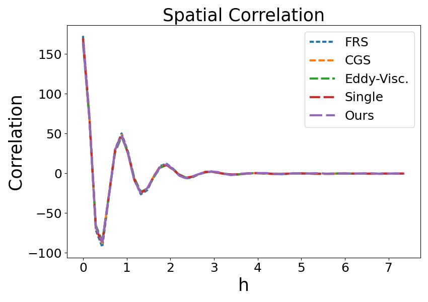
(b) Spatial Correlation

(c) Auto Correlation Coefficient

Figure 4: Experiment Results for KS Equation ’FRS’(blue line) refers to fully-resolved simulation, and serves as ground truth. ’CGS’: coarse-grid simulation(no closure model). ’Eddy-Visc.’: classical eddy-viscosity model. ’Single’: learning-based single-state closure model. Our method (purple) is closest to ground truth among all coarse-grid methods.

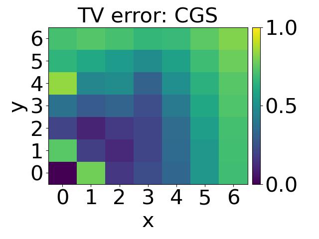
(a) Coarse-grid Simmulation (no closure model)

(b) CGS with Smagorinsky model

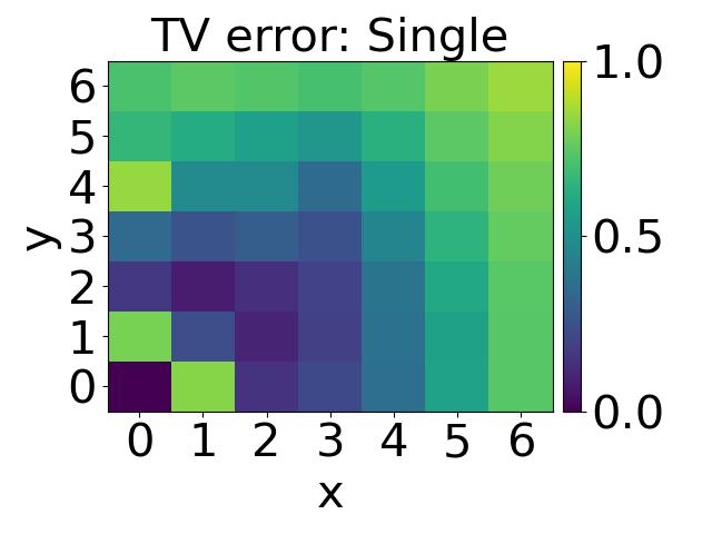
(c) Learning-based single-state model

(d) Our method

Figure 5: TV error for NS Equation The $(k,j)$-element represents the TV error regarding the distribution of the mode length of $(k,j)$ Fourier basis $e^{i\frac{2\pi}{L}(kx+jy)}$.

(a) Coarse-grid Simulation (no closure model))

(b) CGS with Smagorinsky model

(c) Learning-based single-state model

(d) Our method

Figure 6: log-scale TV error for NS Equation The $(k,j)$-element represents the logarithm of TV error regarding the distribution of the mode length of $(k,j)$ Fourier basis $e^{i\frac{2\pi}{L}(kx+jy)}$.

(a) Energy Spectrum

(b) Dissipation Distribution

(c) Vorticity Distribution

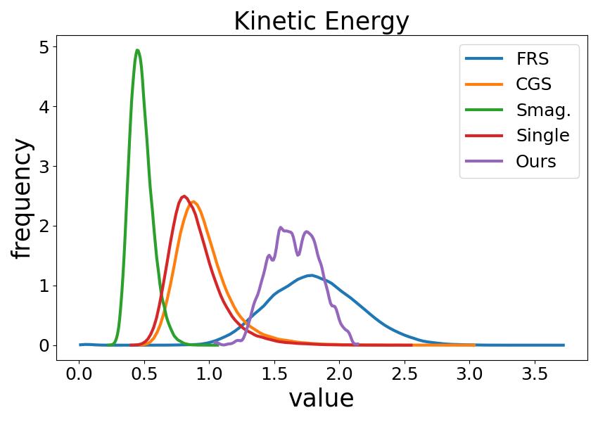
(d) Kinetic Energy Distribution

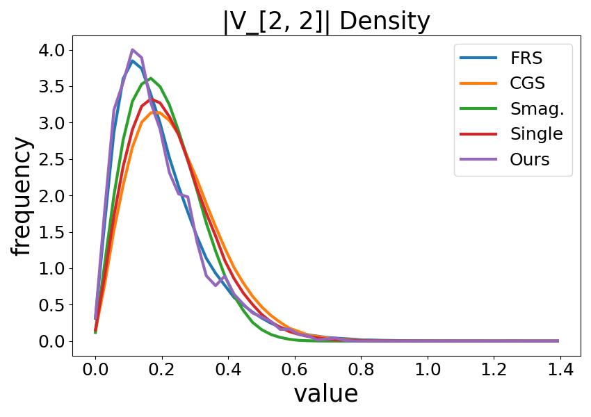
(e) Distribution of component for $(2,2)$ Fourier basis

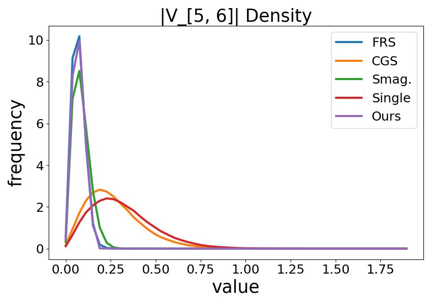
(f) Distribution of component for $(5,6)$ Fourier basis

Figure 7: Experiment Results for NS Equation ’FRS’(blue line) refers to fully-resolved simulation, and serves as ground truth. ’CGS’: coarse-grid simulation(no closure model). ’Smag.’: classical Smagorinsky model. ’Single’: learning-based single-state closure model. Our method (purple) is closest to ground truth among all coarse-grid methods.

G.3 Ablation Study

We carry out an ablation study for KS equation to verify the effect of pertaining with data loss and CGS data loss. The training dataset is described in Appendix E. The results are as in Figure 8.

We conclude that pretraining with data loss is beneficial to the optimization of the PDE loss function and that pretraining with CGS data can improve the generalization property of the model. Even though CGS data is potentially incorrect, it is utilizable for training because they contain some information of the underlying PDE.

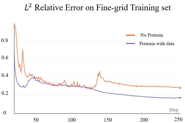
(a)

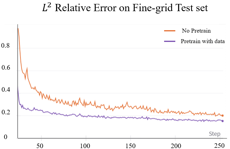
(b)

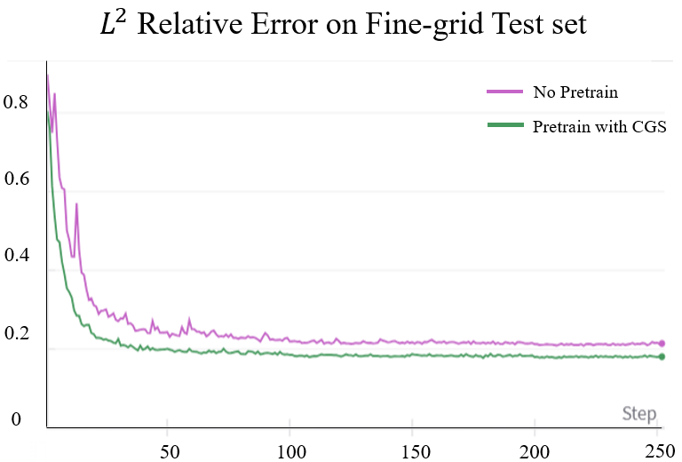
(c)

Figure 8: Experiment Results during training for KS Equation (a)$L^{2}$ relative error on training set for PDE-loss minimization. The optimization achieves a smaller loss when the model has been pre-trained with data loss(purple curve). (b)$L^{2}$ relative error on the test set for PDE-loss minimization. The model achieves a smaller error when it has been pre-trained with data loss(purple curve). (c) $L^{2}$ relative error on the test set for FRS data-loss minimization. The model has better generalization if it has been pre-trained with CGS data loss (green curve).

References

- [1] JAS Lima, R Silva Jr, and Janilo Santos. Plasma oscillations and nonextensive statistics. Physical Review E, 61(3):3260, 2000.
- [2] Gregory Flato, Jochem Marotzke, Babatunde Abiodun, Pascale Braconnot, Sin Chan Chou, William Collins, Peter Cox, Fatima Driouech, Seita Emori, Veronika Eyring, et al. Evaluation of climate models. In Climate change 2013: the physical science basis. Contribution of Working Group I to the Fifth Assessment Report of the Intergovernmental Panel on Climate Change, pages 741–866. Cambridge University Press, 2014.
- [3] Stephen H Schneider and Robert E Dickinson. Climate modeling. Reviews of Geophysics, 12(3):447–493, 1974.
- [4] Jeffrey P Slotnick, Abdollah Khodadoust, Juan Alonso, David Darmofal, William Gropp, Elizabeth Lurie, and Dimitri J Mavriplis. CFD vision 2030 study: a path to revolutionary computational aerosciences. Technical Report CR-2014–21817, NASA, 2014.
- [5] David M Wootton and David N Ku. Fluid mechanics of vascular systems, diseases, and thrombosis. Annual Review of Biomedical Engineering, 1(1):299–329, 1999.
- [6] Julio M Ottino. Mixing, chaotic advection, and turbulence. Annual Review of Fluid Mechanics, 22(1):207–254, 1990.
- [7] Gerald Jay Sussman and Jack Wisdom. Chaotic evolution of the solar system. Science, 257(5066):56–62, 1992.
- [8] Henri Korn and Philippe Faure. Is there chaos in the brain? ii. experimental evidence and related models. Comptes Rendus Biologies, 326(9):787–840, 2003.
- [9] Steven H Strogatz. Nonlinear dynamics and chaos: with applications to physics, biology, chemistry, and engineering. CRC press, 2018.
- [10] Kiran Ravikumar, David Appelhans, and PK Yeung. Gpu acceleration of extreme scale pseudo-spectral simulations of turbulence using asynchronism. In Proceedings of the International Conference for High Performance Computing, Networking, Storage and Analysis, pages 1–22, 2019.
- [11] Tapio Schneider, João Teixeira, Christopher S Bretherton, Florent Brient, Kyle G Pressel, Christoph Schär, and A Pier Siebesma. Climate goals and computing the future of clouds. Nature Climate Change, 7(1):3–5, 2017.
- [12] Javier Jimenez and Robert D Moser. Large-eddy simulations: where are we and what can we expect? AIAA journal, 38(4):605–612, 2000.
- [13] Stephen B Pope. Ten questions concerning the large-eddy simulation of turbulent flows. New Journal of Physics, 6(1):35, 2004.
- [14] Joseph Smagorinsky. General circulation experiments with the primitive equations: I. the basic experiment. Monthly Weather Review, 91(3):99–164, 1963.
- [15] Yupeng Zhang and Kaushik Bhattacharya. Iterated learning and multiscale modeling of history-dependent architectured metamaterials. arXiv preprint arXiv:2402.12674, 2024.
- [16] Burigede Liu, Eric Ocegueda, Margaret Trautner, Andrew M Stuart, and Kaushik Bhattacharya. Learning macroscopic internal variables and history dependence from microscopic models. Journal of the Mechanics and Physics of Solids, 178:105329, 2023.
- [17] Valentina Tozzini. Coarse-grained models for proteins. Current Opinion in Structural Biology, 15(2):144–150, 2005.
- [18] Kenneth G Wilson. Renormalization group and strong interactions. Physical Review D, 3(8):1818, 1971.
- [19] Charles Meneveau and Joseph Katz. Scale-invariance and turbulence models for large-eddy simulation. Annual Review of Fluid Mechanics, 32(1):1–32, 2000.
- [20] Robert D Moser, Sigfried W Haering, and Gopal R Yalla. Statistical properties of subgrid-scale turbulence models. Annual Review of Fluid Mechanics, 53:255–286, 2021.
- [21] Di Zhou and H Jane Bae. Sensitivity analysis of wall-modeled large-eddy simulation for separated turbulent flow. Journal of Computational Physics, 506:112948, 2024.
- [22] Karthik Duraisamy, Gianluca Iaccarino, and Heng Xiao. Turbulence modeling in the age of data. Annual Review of Fluid Mechanics, 51:357–377, 2019.
- [23] Karthik Duraisamy. Perspectives on machine learning-augmented reynolds-averaged and large eddy simulation models of turbulence. Physical Review Fluids, 6(5):050504, 2021.
- [24] Benjamin Sanderse, Panos Stinis, Romit Maulik, and Shady E Ahmed. Scientific machine learning for closure models in multiscale problems: a review. arXiv preprint arXiv:2403.02913, 2024.
- [25] Suryanarayana Maddu, Scott Weady, and Michael J Shelley. Learning fast, accurate, and stable closures of a kinetic theory of an active fluid. Journal of Computational Physics, 504:112869, 2024.
- [26] Varun Shankar, Vedant Puri, Ramesh Balakrishnan, Romit Maulik, and Venkatasubramanian Viswanathan. Differentiable physics-enabled closure modeling for burgers’ turbulence. Machine Learning: Science and Technology, 4(1):015017, 2023.
- [27] Masataka Gamahara and Yuji Hattori. Searching for turbulence models by artificial neural network. Physical Review Fluids, 2(5):054604, 2017.
- [28] Andrea Beck, David Flad, and Claus-Dieter Munz. Deep neural networks for data-driven LES closure models. Journal of Computational Physics, 398:108910, 2019.
- [29] Romit Maulik, Omer San, Adil Rasheed, and Prakash Vedula. Subgrid modelling for two-dimensional turbulence using neural networks. Journal of Fluid Mechanics, 858:122–144, 2019.
- [30] Yifei Guan, Ashesh Chattopadhyay, Adam Subel, and Pedram Hassanzadeh. Stable a posteriori LES of 2D turbulence using convolutional neural networks: Backscattering analysis and generalization to higher re via transfer learning. Journal of Computational Physics, 458:111090, 2022.
- [31] Zongyi Li, Nikola Kovachki, Kamyar Azizzadenesheli, Burigede Liu, Kaushik Bhattacharya, Andrew Stuart, and Anima Anandkumar. Fourier neural operator for parametric partial differential equations. arXiv preprint arXiv:2010.08895, 2020.
- [32] Nikola Kovachki, Zongyi Li, Burigede Liu, Kamyar Azizzadenesheli, Kaushik Bhattacharya, Andrew Stuart, and Anima Anandkumar. Neural operator: Learning maps between function spaces with applications to PDEs. Journal of Machine Learning Research, 24(89):1–97, 2023.
- [33] Zongyi Li, Hongkai Zheng, Nikola Kovachki, David Jin, Haoxuan Chen, Burigede Liu, Kamyar Azizzadenesheli, and Anima Anandkumar. Physics-informed neural operator for learning partial differential equations. ACM/JMS Journal of Data Science, 2021.
- [34] Anudhyan Boral, Zhong Yi Wan, Leonardo Zepeda-Núñez, James Lottes, Qing Wang, Yi-fan Chen, John Roberts Anderson, and Fei Sha. Neural ideal large eddy simulation: Modeling turbulence with neural stochastic differential equations. arXiv preprint arXiv:2306.01174, 2023.
- [35] William C Reynolds. The potential and limitations of direct and large eddy simulations. In Whither Turbulence? Turbulence at the Crossroads: Proceedings of a Workshop Held at Cornell University, Ithaca, NY, March 22–24, 1989, pages 313–343. Springer, 2005.
- [36] Haecheon Choi and Parviz Moin. Grid-point requirements for large eddy simulation: Chapman’s estimates revisited. Physics of Fluids, 24(1), 2012.
- [37] Qian Wang, Nicolò Ripamonti, and Jan S Hesthaven. Recurrent neural network closure of parametric pod-galerkin reduced-order models based on the mori-zwanzig formalism. Journal of Computational Physics, 410:109402, 2020.
- [38] Justin Sirignano and Jonathan F MacArt. Dynamic deep learning LES closures: Online optimization with embedded DNS. arXiv preprint arXiv:2303.02338, 2023.
- [39] Samuel Lanthaler, Zongyi Li, and Andrew M Stuart. The nonlocal neural operator: Universal approximation. arXiv preprint arXiv:2304.13221, 2023.
- [40] Chao Ma, Jianchun Wang, et al. Model reduction with memory and the machine learning of dynamical systems. arXiv preprint arXiv:1808.04258, 2018.
- [41] Roger Temam. Infinite-dimensional dynamical systems in mechanics and physics, volume 68. Springer Science & Business Media, 2012.
- [42] John Milnor. On the concept of attractor. Communications in Mathematical Physics, 99:177–195, 1985.
- [43] Sergei P Kuznetsov. Dynamical chaos and uniformly hyperbolic attractors: from mathematics to physics. Physics-Uspekhi, 54(2):119, 2011.
- [44] Simona Dinicola, Fabrizio D’Anselmi, Alessia Pasqualato, Sara Proietti, Elisabetta Lisi, Alessandra Cucina, and Mariano Bizzarri. A systems biology approach to cancer: fractals, attractors, and nonlinear dynamics. Omics: a journal of integrative biology, 15(3):93–104, 2011.
- [45] Sui Huang, Ingemar Ernberg, and Stuart Kauffman. Cancer attractors: a systems view of tumors from a gene network dynamics and developmental perspective. In Seminars in cell & developmental biology, volume 20, pages 869–876. Elsevier, 2009.
- [46] Alfredo Medio and Marji Lines. Nonlinear dynamics: A primer. Cambridge University Press, 2001.
- [47] Justin Sirignano, Jonathan F MacArt, and Jonathan B Freund. Dpm: A deep learning pde augmentation method with application to large-eddy simulation. Journal of Computational Physics, 423:109811, 2020.
- [48] Björn List, Li-Wei Chen, and Nils Thuerey. Learned turbulence modelling with differentiable fluid solvers: physics-based loss functions and optimisation horizons. Journal of Fluid Mechanics, 949:A25, 2022.
- [49] Fei Lu, Kevin K Lin, and Alexandre J Chorin. Data-based stochastic model reduction for the kuramoto–sivashinsky equation. Physica D: Nonlinear Phenomena, 340:46–57, 2017.
- [50] Jacob A Langford and Robert D Moser. Optimal LES formulations for isotropic turbulence. Journal of Fluid Mechanics, 398:321–346, 1999.
- [51] Matthew Levine and Andrew Stuart. A framework for machine learning of model error in dynamical systems. Communications of the American Mathematical Society, 2(07):283–344, 2022.
- [52] Benedikt Barthel Sorensen, Alexis Charalampopoulos, Shixuan Zhang, Bryce Harrop, Ruby Leung, and Themistoklis Sapsis. A non-intrusive machine learning framework for debiasing long-time coarse resolution climate simulations and quantifying rare events statistics. arXiv preprint arXiv:2402.18484, 2024.
- [53] Vivek Oommen, Khemraj Shukla, Saaketh Desai, Remi Dingreville, and George Em Karniadakis. Rethinking materials simulations: Blending direct numerical simulations with neural operators. arXiv preprint arXiv:2312.05410, 2023.
- [54] Hugo Frezat, Guillaume Balarac, Julien Le Sommer, and Ronan Fablet. Gradient-free online learning of subgrid-scale dynamics with neural emulators. arXiv preprint arXiv:2310.19385, 2023.
- [55] Lu Lu, Pengzhan Jin, Guofei Pang, Zhongqiang Zhang, and George Em Karniadakis. Learning nonlinear operators via deeponet based on the universal approximation theorem of operators. Nature Machine Intelligence, 3(3):218–229, 2021.
- [56] George Em Karniadakis, Ioannis G Kevrekidis, Lu Lu, Paris Perdikaris, Sifan Wang, and Liu Yang. Physics-informed machine learning. Nature Reviews Physics, 3(6):422–440, 2021.
- [57] Pratik Rathore, Weimu Lei, Zachary Frangella, Lu Lu, and Madeleine Udell. Challenges in training pinns: A loss landscape perspective. arXiv preprint arXiv:2402.01868, 2024.
- [58] Chuwei Wang, Shanda Li, Di He, and Liwei Wang. Is physics informed loss always suitable for training physics informed neural network? Advances in Neural Information Processing Systems, 35:8278–8290, 2022.
- [59] Pritpal Matharu and Bartosz Protas. Optimal closures in a simple model for turbulent flows. SIAM Journal on Scientific Computing, 42(1):B250–B272, 2020.
- [60] Cédric Villani et al. Optimal transport: old and new, volume 338. Springer, 2009.
- [61] Filippo Santambrogio. Optimal transport for applied mathematicians. Birkäuser, NY, 55(58-63):94, 2015.
- [62] Michel Ledoux and Michel Talagrand. Probability in Banach Spaces: isoperimetry and processes. Springer Science & Business Media, 2013.
- [63] Nicholas Vakhania, Vazha Tarieladze, and S Chobanyan. Probability distributions on Banach spaces, volume 14. Springer Science & Business Media, 2012.
- [64] Michael Brin and Garrett Stuck. Introduction to dynamical systems. Cambridge university press, 2002.
- [65] Lan Wen. Differentiable dynamical systems, volume 173. American Mathematical Soc., 2016.
- [66] Isaac P Cornfeld, Sergej V Fomin, and Yakov Grigorevich Sinai. Ergodic theory, volume 245. Springer Science & Business Media, 2012.
- [67] Roger Temam. Navier-Stokes equations: theory and numerical analysis, volume 343. American Mathematical Soc., 2001.
- [68] Qiqi Wang, Rui Hu, and Patrick Blonigan. Least squares shadowing sensitivity analysis of chaotic limit cycle oscillations. Journal of Computational Physics, 267:210–224, 2014.
- [69] Sergey P Kuznetsov. Hyperbolic chaos. Springer, 2012.
- [70] Stephen Smale. An infinite dimensional version of Sard’s theorem. In The Collected Papers of Stephen Smale: Volume 2, pages 529–534. World Scientific, 2000.
- [71] Aly-Khan Kassam and Lloyd N Trefethen. Fourth-order time-stepping for stiff PDEs. SIAM Journal on Scientific Computing, 26(4):1214–1233, 2005.
- [72] Gary J Chandler and Rich R Kerswell. Invariant recurrent solutions embedded in a turbulent two-dimensional kolmogorov flow. Journal of Fluid Mechanics, 722:554–595, 2013.
- [73] Alexey Dosovitskiy, Lucas Beyer, Alexander Kolesnikov, Dirk Weissenborn, Xiaohua Zhai, Thomas Unterthiner, Mostafa Dehghani, Matthias Minderer, Georg Heigold, Sylvain Gelly, et al. An image is worth 1616 words: Transformers for image recognition at scale. arXiv preprint arXiv:2010.11929, 2020.
- [74] Ilya Loshchilov and Frank Hutter. Decoupled weight decay regularization. arXiv preprint arXiv:1711.05101, 2017.
- [75] J-P Eckmann and David Ruelle. Ergodic theory of chaos and strange attractors. Reviews of Modern Physics, 57(3):617, 1985.