Gravitational Waves and Dark Matter in the Gauged Two-Higgs Doublet Model
Abstract
We investigate the possibility of a strong first-order electroweak phase transition during the early universe within the framework of the gauged two-Higgs doublet model (G2HDM) and explore its detectability through stochastic gravitational wave signals. The G2HDM introduces a dark replica of the Standard Model electroweak gauge group, inducing an accidental symmetry which not only leads to a simple scalar potential at tree-level but also offers a compelling vectorial dark matter candidate. Using the high temperature expansion in the effective potential that manifests gauge invariance, we find a possible two-step phase transition pattern in the model with a strong first-order transition occurring in the second step at the electroweak scale temperature. Collider data from the LHC plays a crucial role in constraining the parameter space conducive to this two-step transition. Furthermore, satisfying the nucleation condition necessitates the masses of scalar bosons in the hidden sector to align with the electroweak scale, potentially probed by future collider detectors. The stochastic gravitational wave energy spectrum associated with the phase transition is computed. The results indicate that forthcoming detectors such as BBO, LISA, DECIGO, TianQin and Taiji could potentially detect the gravitational wave signals generated by the first-order phase transition. Additionally, we find that the parameter space probed by gravitational waves can also be searched for in future dark matter direct detection experiments, in particular those designed for dark matter masses in the sub-GeV range using the superfluid Helium target detectors.
I Introduction
Unraveling the thermal history of electroweak symmetry breaking is considered a crucial task in both particle physics and cosmology. In the Standard Model (SM), EW symmetry breaking proceeds through a smooth crossover as indicated by lattice simulations Kajantie et al. (1996a); Rummukainen et al. (1998); Laine and Rummukainen (1999); Aoki et al. (1999). However, a first-order electroweak phase transition (FOEWPT) can occur in many BSM theories, such as singlet scalar extensions McDonald (1994); Profumo et al. (2007); Cline et al. (2009); Espinosa et al. (2012a); Cline and Kainulainen (2013a); Alanne et al. (2014); Curtin et al. (2014); Profumo et al. (2015); Huang and Li (2015); Kotwal et al. (2016); Vaskonen (2017); Ghorbani (2017); Cline et al. (2017); Beniwal et al. (2017); Kurup and Perelstein (2017); Chiang et al. (2018); Carena et al. (2019, 2018); Grzadkowski and Huang (2018); Huang et al. (2018a); Alves et al. (2019); Ghorbani and Ghorbani (2020); Cheng and Bian (2018); Alanne et al. (2020); Gould et al. (2019); Carena et al. (2020); Li et al. (2019); Bell et al. (2019), triplet scalar extensions Inoue et al. (2016); Niemi et al. (2019); Chala et al. (2019); Zhou et al. (2019), two-Higgs doublet models Bochkarev et al. (1990); McLerran et al. (1991); Bochkarev et al. (1991); Turok and Zadrozny (1991); Cohen et al. (1991); Turok and Zadrozny (1992); Nelson et al. (1992); Funakubo et al. (1994); Davies et al. (1994); Cline et al. (1996); Funakubo et al. (1995, 1996); Cline and Lemieux (1997); Fromme et al. (2006); Cline et al. (2011); Dorsch et al. (2013); Cline and Kainulainen (2013b); Dorsch et al. (2014); Fuyuto and Senaha (2015); Chao and Ramsey-Musolf (2015); Fuyuto et al. (2016); Chiang et al. (2016); Haarr et al. (2016); Dorsch et al. (2017a); Basler et al. (2017); Fuyuto et al. (2018); Dorsch et al. (2017b); Cherchiglia and Nishi (2017); Basler et al. (2018); Andersen et al. (2018); Bernon et al. (2018); Huang and Yu (2018); Gorda et al. (2019); Basler and Mühlleitner (2019); Modak and Senaha (2019); Wang et al. (2019, 2020); Kainulainen et al. (2019); Paul et al. (2021); Su et al. (2021), supersymmetric models Apreda et al. (2002); Huber et al. (2016); Huber and Konstandin (2008a); Demidov et al. (2018), left-right symmetric models Brdar et al. (2019); Li et al. (2021), Pati-Salam model Huang et al. (2020), Georgi-Machacek model Chiang and Yamada (2014); Zhou et al. (2019), Zee-Babu model Phong et al. (2018, 2022), composite Higgs models Espinosa et al. (2012b); Chala et al. (2016, 2019); Bruggisser et al. (2018a, b); Bian et al. (2019); De Curtis et al. (2019); Xie et al. (2020), neutrino mass models Di Bari et al. (2021); Zhou et al. (2022) and hidden sector models involving scalars Schwaller (2015); Baldes and Garcia-Cely (2019); Breitbach et al. (2019); Croon et al. (2018); Baldes (2017); Croon et al. (2020); Hall et al. (2023, 2020); Chao et al. (2021); Dent et al. (2022), etc. In some cases, the FOEWPT can occur in multiple steps Weinberg (1974); Land and Carlson (1992); Patel and Ramsey-Musolf (2013); Patel et al. (2013); Blinov et al. (2015); Niemi et al. (2019); Croon and White (2018); Morais et al. (2020); Morais and Pasechnik (2020); Angelescu and Huang (2019); Friedrich et al. (2022).
Apart from being of interest in its own right, the occurrence of FOEWPT fulfills one of the conditions established by Sakharov Sakharov (1967) for the realization of the electroweak baryogenesis mechanism Trodden (1999); Cline (2006); Morrissey and Ramsey-Musolf (2012); White (2016); Garbrecht (2020) which accounts for the observed cosmological matter-antimatter asymmetry. A FOEWPT also admits a rich array of possible experimentally observable signatures. In particular, the presence of BSM physics related to a FOEWPT can have an impact on the properties of the Higgs boson and predicts the existence of new scalar particles with masses at or below the TeV scale, which may be probed by future collider experiments (see e.g. Ramsey-Musolf (2020); Carena et al. (2023); Wang et al. (2022); Zhang et al. (2023); Wang et al. (2023a) and references therein). Apart from undergoing a strong FOEWPT, these new physics models often provide candidates for dark matter (DM), see e.g. Chowdhury et al. (2012); Katz et al. (2015); Fabian et al. (2021); Bell et al. (2020); Chiang et al. (2021); Zhang et al. (2024). Furthermore, a FOEWPT can result in the formation of bubble nucleation, which can expand and collide, producing stochastic gravitational waves (GWs) (see Weir (2018) for a brief review). This GW signal is potentially within the reach of upcoming space-based laser interferometer GW detectors, such as LISA Amaro-Seoane et al. (2017); Robson et al. (2019), BBO Crowder and Cornish (2005), TianQin Luo et al. (2016); Hu et al. (2017), Taiji Hu and Wu (2017); Ruan et al. (2020) and DECIGO Kawamura et al. (2006, 2011); Musha (2017).
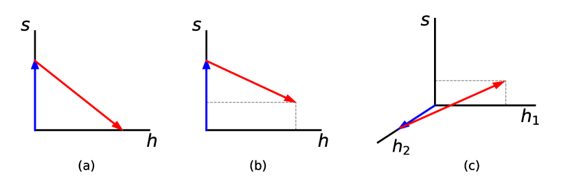
One of the most straightforward extensions to SM involves the presence of a real singlet scalar field alongside the SM Higgs doublet field, accompanied by the imposition of a discrete symmetry. In such the framework, it can admit a strong FOEWPT in the two-step phase transition as depicted in the left panel of Fig. 1 — where () represents classical background field of the singlet (SM doublet) Ghorbani (2021) 111Derived from an analysis of the high-temperature expansion of the thermal effective potential.. In the case of spontaneous breaking Carena et al. (2020), the inclusion of the cubic term () in the effective potential can allow for the occurrence of a FOEWPT through as depicted in the center panel of Fig. 1. However, it is worth noting that the presence of this cubic term is subject to the issue of gauge dependence Patel and Ramsey-Musolf (2011). Nevertheless, to facilitate these transitions, the mass of the singlet scalar must be confined to be light. In particular, necessitating the occurrence of a two-step EWPT like the left panel of Fig. 1 requires
| (1) |
where is the critical temperature in the first (second) step and is the temperature at electroweak (EW) scale. If the symmetry is preserved at zero temperature (left panel of Fig. 1), the scalar singlet acquires its mass solely from the SM VEV. The requirement in (1) sets the scalar singlet mass to be below 700 GeV Ramsey-Musolf (2020). On the other hand, for the spontaneous breaking case (center panel of Fig. 1), the scalar singlet mass is confined to below 50 GeV and the associated GW signals are typically too low to be probed by future GW detectors Carena et al. (2020).
Furthermore, for the symmetry preserving model, where the singlet scalar gets zero vacuum expectation value (VEV) at zero temperature, the singlet scalar can remain stable and serve as a DM candidate. This straightforward extension of SM incorporating a symmetric potential allows us to perform gauge-invariant and scale-invariant treatments of EWPT computation. However, except for small DM mass in the range of GeV that can be probed by future colliders, this scenario is ruled out by direct detection experiments Ghorbani (2021).
We thus ask following questions:
-
•
In what context the upper limit on the new scalar mass due to the requirement of the two-step FOEWPT can be relaxed?
-
•
Can such the model yield a DM candidate that satisfies the correct DM relic abundance and evades current DM direct detection constraints?
-
•
Can the GW signals generated from FOEWPT detectable at forthcoming GW detectors and how does it interplay with DM direct detection signals?
In this analysis, we address these questions within the framework of a simplified G2HDM Ramos et al. (2021a, b) which is based on the original version proposed in Huang et al. (2016a). In addition to the SM doublet and singlet scalars , this model incorporates an extra inert doublet . While inert at zero temperature, this inert doublet can develop a background field (i.e., VEV) at high temperature (high-T), resulting in rich phase transition patterns. Using the high-T expansion approximation in the effective potential that manifests gauge invariance, we find a particularly novel and interesting two-step phase transition, with the first step leading to the inert doublet vacuum and the subsequent step returning to the true EW vacuum with non-zero SM doublet and singlet scalar VEVs as depicted schematically in the right panel of Fig. 1. The first-order phase transition may take place in the second step. In the second step the singlet can develop a new VEV along with the SM VEV from , thereby providing additional contributions to the masses of new scalars. This can lead to a relaxation of the upper bounds on masses of extra scalars in the model while archiving the two-step FOEWPT.
Moreover, the model naturally accommodates a hidden -parity, if not spontaneously broken at zero temperature, ensuring that the lightest -parity odd particle serves as the DM candidate. The DM candidate in the model can be either a complex scalar Chen et al. (2020), a hidden heavy neutrino, or a non-abelian vector gauge boson — all of which are electrically neutral and possess odd -parity. In this work, we will focus on the hidden gauge bosons as the DM candidate Ramos et al. (2021a, b).
We demonstrate that the stochastic GW signals from the two-step FOEWPT in the simplified G2HDM can be probed in future GW experiments. The predictions of GW signals in this study are derived from the high-T expansion approximation in the one-loop effective potential, which preserves gauge invariance. To attain more accurate results and ensure a realistic perturbative treatment Patel and Ramsey-Musolf (2011), it is imperative to incorporate a two-loop finite temperature effective potential which has yet been computed for G2HDM. Our investigation reveals that the parameter space accessible through GWs can also be explored in upcoming DM direct detection experiments. Specifically, we highlight the relevance of experiments tailored for detecting DM with masses in the sub-GeV range, utilizing superfluid Helium target detectors.
The layout of this paper is as follows. In Sec. II, we will briefly review the simplified version of G2HDM and its phenomenological constraints. In Sec. III, after a succinct review of the current status of theoretical EWPT computation, we present our analysis in G2HDM using the high-T expansion of the finite temperature effective potential in order to maintain gauge invariance. We focus on the two-step transition pattern and identify parameter space where the desired pattern can occur. In Sec. IV, we present the stochastic GW prediction signals for the FOEWPT. In Sec. V, we discuss the DM direct detection probes. We conclude in Sec. VI. Six appendices are compiled for (A) field dependent masses, (B) thermal masses, (C) thermal integrals, (D) gauge invariant method beyond leading order computation and scale dependence of the effective potential at finite temperature, (E) critical temperatures, and (F) renormalization group equations.
II The Simplified G2HDM
In this section, we will briefly review the simplified version of G2HDM Ramos et al. (2021a, b). Unlike the original G2HDM presented in Huang et al. (2016a), the simplified version has omitted the triplet scalar , thereby simplifying the scalar potential. The scalar sector in the simplified G2HDM consists of the SM Higgs doublet and a second inert Higgs doublet of , as well as a hidden doublet of . Regarding the two doublets and , the model is different from the popular inert Higgs doublet model (IHDM) in that they are combined into a doublet of the hidden . Their extended electroweak quantum numbers and -parity are summarized in Table 1 for reference.
| Scalar | -parity | ||||
|---|---|---|---|---|---|
| 2 | |||||
| 1 | 2 | 0 |
We note that the model also consists of heavy hidden fermions for the cancellations of gauge and gravitational anomalies. The hidden doublet of can provide realistic Yukawa couplings and mass spectra for the extra fermions and vector bosons. The loop-induced flavor changing neutral current (FCNC) processes within the model have also been investigated Tran and Yuan (2023); Liu et al. (2024). Additionally, the G2HDM is capable of addressing the recent high precision measurement of the boson mass at the CDF II detector Tran et al. (2023). Many other phenomenological aspects of the model have been explored as well in Huang et al. (2016b); Arhrib et al. (2018); Huang et al. (2019, 2018b); Chen et al. (2019); Dirgantara and Nugroho (2022). A pure dark gauge-Higgs sector of with the dark gauge bosons implemented as a self-interacting DM candidate was recently pursued in Tran et al. (2024).
II.1 Higgs Potential and Spontaneous Symmetry Breaking
The most general Higgs potential which is invariant under the extended electroweak gauge group is given by
| (2) |
where (, , , ) and (, ) refer to the and indices respectively, all of which run from 1 to 2, and .
To study general spontaneous symmetry breaking (SSB) at finite temperature, we parameterize the fields according to standard practice
| (3) |
| (4) |
where and are the only nonvanishing temperature dependent classical background field components in and fields respectively. The temperature dependence in the background fields is implicit.
In terms of the background fields, the effective potential at tree level is
| (5) | |||||
Note that in the tree level effective potential, the term and all the terms involving the coupling are absent.
II.2 Mass spectrum and mixing at tree level
At zero temperature, the classical background fields are the constant vacuum expectation values (VEVs) i.e. and . Since is odd under -parity, it plays the role as the inert Higgs doublet at zero temperature, so . With this set up, a -parity protects the stability of DM candidate in the model Ramos et al. (2021a, b). The scalar potential at tree level given in Eq. (5) becomes
| (6) |
From the -parity assignment given in Table 1, we note that while there is no mixing between and , () can mix with the lower (upper) component of . Specifically, the neutral components and in and , respectively, are both even under -parity and can combine to form two observable Higgs fields, denoted as and . This mixing can be given as
| (7) |
where the mixing angle is given by
| (8) |
The masses of and are given by
| (9) | |||||
The observed Higgs boson (which we denote as ) at the LHC is either or , depending on their masses (9) determined by the underlying portal parameters in the scalar potential. Currently, the most precise determination of the Higgs boson mass is GeV, as reported in Ref. Sirunyan et al. (2020).
Furthermore, the -parity odd fields and can mix to produce two fields: a physical dark Higgs boson denoted as , and an unphysical Goldstone boson that gets absorbed by the boson. The mixing is given by
| (10) |
where the mixing angle satisfies
| (11) |
and the mass of is
| (12) |
is the Goldstone field associated with the gauge boson (). Its mass depends on the gauge fixings Ramos et al. (2021a). In Feynman-’t Hooft gauge it has the same mass as the (). In Landau and unitary gauge, its mass is zero and infinite respectively.
The charged Higgs , same as at zero temperature, is also -parity odd and has a mass
| (13) |
We note that the quartic coupling parameters in the scalar potential that determine the masses of -parity odd states and are different from those of -parity even states and .
The gauge bosons have a mass
| (14) |
where is the gauge coupling of . are both electrically neutral and odd under -parity. Therefore, they could potentially serve as dark matter candidates, provided that their mass is the lightest among all odd -parity particles.
Finally the SM boson mixes with the gauge field associated with the third generator of and the gauge field (see Ref. Ramos et al. (2021a, b) for the mass matrix). This leads to three physical fields for . We will identify with the neutral gauge boson resonance observed at LEP with a mass of 91.1876 GeV Zyla et al. (2020a), while the other two states can be identified as the dark photon () and the dark boson () with the ordering .
The fundamental parameters in the scalar potential can be expressed in terms of particle masses by performing an inversion, as demonstrated in Refs. Ramos et al. (2021a, b); Tran and Yuan (2023):
| (15) | |||||
| (16) | |||||
| (17) | |||||
| (18) | |||||
| (19) | |||||
| (20) |
From (14), we also obtain
| (21) |
Thus one can use , , , , and as input in our numerical scan. The additional free parameters in the model are the heavy hidden fermion mass , the gauge coupling and the Stueckelberg mass .
II.3 Constraints
The constraints on the model have been studied in Ramos et al. (2021a, b); Tran and Yuan (2023), taking into account the theoretical constraints on the scalar potential, as well as constraints from Higgs measurements at the LHC, electroweak precision data, dark photon and dark matter searches. Here we summarize these constraints as follows.
Theoretical constraints:
(a) Vacuum Stability: To ensure that the scalar potential has a minimum value, we adopt the copositivity conditions suggested by Arhrib et al. (2018), which provide the following set of constraints on the scalar potential parameters
| (22) |
where and with and .
(b) Perturbative Unitarity: The condition for perturbative unitarity, as presented in Arhrib et al. (2018); Ramos et al. (2021a, b), provides the following constraints
| (23) | |||
| (24) | |||
| (25) | |||
| (26) |
We note that the perturbativity bound can be crucial in some BSM Higgs scenarios, such as the real triplet scalar extension model Bell et al. (2020). However, to impose this constraint, two-loop renormalization group equations are required. We defer to future work an evaluation of the two-loop -functions and corresponding perturbativity constraints, keeping in mind that the latter may lead to further reductions in the viable parameter space.
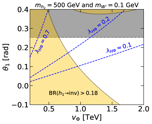
Higgs data constraints : The mixing between -parity even scalar bosons, (Higgs boson) and , results in modifications on the couplings between the Higgs boson and SM particles as compared with those in the SM. Moreover, in addition to contributions from the SM charged particles, the process receives contributions from hidden charged fermions and charged Higgs in the G2HDM. The analytical formulation of this 1-loop process is presented in Tran and Yuan (2023). Utilizing the Higgs signal strength data of the decays into and from CMS measurement CMS-Collaboration (2020), we derive a constraint on the mixing angle, finding that . When combining Higgs signal strength data from both CMS CMS-Collaboration (2020) and ATLAS ATL (2021), a more stringent limit of is established, which is depicted as a gray shaded area in Fig. 2.
We consider the gauge boson with a sub-GeV mass range as the DM candidate in the model, as studied in Ramos et al. (2021a, b). Therefore, (identified as here) can decay invisibly into a pair of . The invisible branching ratio can be given by
| (27) |
where is the total decay width of the 125.38 GeV Higgs boson, MeV is the SM decay width and is its invisible decay width. The latter is given by
| (28) |
with . Recently, CMS set a limit of at C.L., assuming that the Higgs boson production cross-section via vector boson fusion is comparable to the SM prediction Tumasyan et al. (2022). The exclusion region from the Higgs invisible decays is shown on the () plane as the yellow shaded region in Fig. 2.
Combining the constraints from the Higgs signal strengths and Higgs invisible width yields a lower bound on and an upper bound on the Higgs portal parameter , as illustrated in Fig. 2. Specifically, for fixed values of GeV and GeV, the collider data require GeV and .
As we will see later the Higgs portal parameter can have a significant impact on the tree-level effects of the first-order electroweak phase transition. A relatively large value of is required to have a substantial effect Blinov et al. (2015). By combining this requirement with the Higgs signal strength data, an upper bound on can be derived. For instance, our results show that if a first-order electroweak phase transition necessitates , it leads to a constraint of TeV, as demonstrated in Fig. 2.
Electroweak precision and dark photon/ measurements:
We consider constraints from electroweak precision measurements at the pole Zyla et al. (2020a), as well as from Aad et al. (2019) and dark photon physics (see Fabbrichesi et al. (2020) for a recent review). For the specific range of light dark photon and masses, i.e., , considered in this study, these constraints require the new gauge couplings and to be less than Ramos et al. (2021a, b). In this analysis, we also follow Ref. Tran and Yuan (2023) to take into account the recent boson mass measurement at the CDF II Aaltonen et al. (2022).
DM constraints:
(a) Relic density: The main annihilation process of a (sub-)GeV DM is via s-channel, mediated by and . However, due to the smallness of the gauge couplings and , the cross sections of such processes are typically suppressed except in the resonant regions where the mediator masses are approximately twice the DM mass, as discussed in Ramos et al. (2021a, b). In fact, the annihilation process with a heavier mediator near the resonance can account for the observed DM relic density, from the Planck Collaboration Aghanim et al. (2020). Here we utilize micrOMEGAs package Bélanger et al. (2018) to calculate the DM relic density.
(b) Direct detection: The DM can scatter off the target material in underground detectors resulting in a recoil energy that can be detected. The scattering cross section between the DM and the nucleon is dominated by the dark photon mediation process, as the dark photon is considered to have the lightest mass among the mediators Ramos et al. (2021a, b). We again use micrOMEGAs package to calculate the DM-nucleon scattering cross section. The results of the cross section are compared against recent upper limits from experiments including CRESST III Angloher et al. (2017), DarkSide-50 Agnes et al. (2018, 2023), XENON1T Aprile et al. (2018, 2019), XENONnT Aprile et al. (2023) , PandaX-4T Meng et al. (2021) and LZ Aalbers et al. (2023).
(c) Indirect detection and mono-jet: as shown in Ramos et al. (2021a, b), the results of electroweak precision measurements lead to a suppression of the new gauge couplings, resulting in a small DM annihilation cross section that easily satisfies the canonical limits set for various channels by Fermi-LAT data Ackermann et al. (2015); Albert et al. (2017). Furthermore, this suppression of the gauge couplings also leads to a minuscule production cross section for the mono-jet signal at the LHC Ramos et al. (2021a, b). Thus we do not include the constraints from indirect detection and mono-jet in this analysis.
III Electroweak Phase Transition
In the literature, a common approach to calculate the EWPT is through the use of perturbation theory. However, this method becomes unreliable at temperatures due to infrared (IR) bosonic contribution to thermal loops Linde (1980), which can cause a breakdown of the theory near the phase transition. Apart from this inherent shortcoming, the reliability of perturbative computations can be improved using the well-known daisy resummation Arnold (1992); Parwani (1992), though the convergence remains slow. Recent attempts to improve the thermal resummation have been performed in Refs. Curtin et al. (2018, 2024). Additionally, the conventional perturbative studies are often challenged by gauge dependence issues Patel and Ramsey-Musolf (2011); Wainwright et al. (2011). Efforts in Refs. Laine (1995); Patel and Ramsey-Musolf (2011) have been made to remove this gauge dependence which is guaranteed by the Nielsen identities Nielsen (1975); Fukuda and Kugo (1976). The choice of renormalization scheme and renormalization scale can also introduce additional uncertainties, leading to theoretical predictions that can vary significantly Croon et al. (2021); Gould and Tenkanen (2021); Athron et al. (2023).
A more systematic approach to include thermal resummation is through the use of the dimensionally reduced 3d effective field theory (EFT)Kajantie et al. (1996b); Farakos et al. (1995). Recently, an automated package has been developed for this Ekstedt et al. (2023). The use of the dimensional reduced 3d EFT in the calculation of the EWPT has been studied in models such as the triplet model Niemi et al. (2019); Friedrich et al. (2022). Efforts have also been made to combine thermal resummation with gauge invariance using the dimensional reduced 3d EFT Kainulainen et al. (2019); Croon et al. (2021); Niemi et al. (2021a); Gould and Tenkanen (2021); Schicho et al. (2022). Another combination of thermal resummation and gauge invariance has also been developed recently Ekstedt and Löfgren (2020), which uses the 4d perturbation theory with a consistent power counting. Ultimately, one must rely on non-perturbative (lattice) computations to fully include the important bosonic IR contributions. For recent studies of the EWPT using Monte Carlo simulations, see Refs. Gould et al. (2019); Niemi et al. (2021b); Gould et al. (2022); Niemi et al. (2024). Importantly, one requires such lattice studies to determine the parameter-space boundary between a bona fide phase transition and a smooth crossover. In what follows, we rely on perturbation theory to identify the potentially FOWEPT-viable regions of parameter space, and defer a complete non-perturbative study to the future.
III.1 One Loop Finite Temperature Effective Potential With Daisy Resummation
The one loop correction can be split into several pieces
| (30) | |||||
The first term is the Coleman-Weinberg effective potential Coleman and Weinberg (1973); Weinberg (1973) which is temperature independent, the second term is finite temperature correction, and the third term is the counter term. The Coleman-Weinberg effective potential in dimensional regularization can be expressed as
| (31) |
where denotes the field dependent mass (See Appendix A) of the particle with spin and number of degree of freedom ; for scalars and fermions and for gauge bosons;
| (32) |
with denotes the Euler-Mascheroni constant; is a renormalization scale (See Appendix F). The finite temperature correction piece is Dolan and Jackiw (1974); Weinberg (1974)
| (33) |
Here is the one loop thermal function (with daisy resummation) defined by (99) in Appendix C. In the G2HDM, we have to sum over the following 3 sets of particles inside the loop
| (34) |
| (35) |
| (36) |
In (34), and are the CP-even and CP-odd scalars respectively. In (35), are the mass eigenstates of the massive neutral gauge bosons. For the general mass spectra of the model, see Appendix A for details. The corresponding degrees of freedom are
We note that due to the thermal mass corrections for the scalars and the longitudinal gauge bosons, the summation in Eq. (33) has to be treated slightly different from the summation in Eq. (III.1) as given explicitly in (99). This is the result of the daisy resummation Arnold and Espinosa (1993); Carrington (1992).
In order to facilitate the analysis of the phase transition, we limit our consideration to the leading terms of the thermal correction functions and for the boson and fermion respectively. As a result, the thermal effective potential can be expressed in this high-T expansion as follows:
| (37) |
where , and are the thermal mass corrections for the scalar fields and their formulas are provided by (B), (87) and (88) respectively in Appendix B.
III.2 Thermal history
Given the three possible non-zero VEVs , there are eight combinations of possible extrema. To ensure the stability of the dark matter candidate, it is necessary that at zero temperature, thereby restoring the -parity in the model Ramos et al. (2021b, a). We first note that, with a high-T expansion of the effective potential given in Eq. (37), a single-step transition to the electroweak vacuum, i.e., , cannot be of first-order type. This is due to conflicting requirements that arise from the need for both and to be real and non-zero, as well as the positivity and minimum conditions of the scalar potential at zero temperature Ghorbani (2021).
After thoroughly scanning the parameter space in the model, we find a phase transition pattern that satisfies the electroweak vacuum requirement and leads to a strong first-order phase transition, as illustrated in the right panel of Fig. 1 where , and . This pattern involves two-steps: , where the first step is a second-order phase transition, and the second is a first-order phase transition. We note that other two-step transition patterns are possible; however, these patterns may not result in a strong first-order phase transition. For instance, for the transition patterns of and , the scalar potential in Eq. (37) can be reduced to the one that is the same as in a real singlet scalar extension model with symmetry, wherein the two-step transition ended up with two non-zero VEVs cannot generate a first-order phase transition Ghorbani (2021). We would like to mention that multiple-step transitions beyond two-step transitions can occur, and a first-order phase transition can arise among these steps. However, for this analysis, we have restricted ourselves to the two-step EWPT.
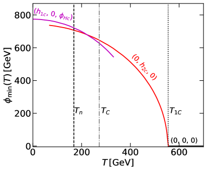
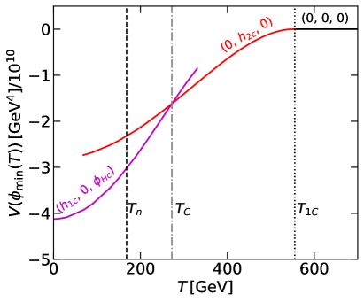
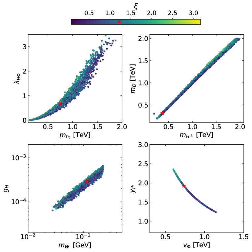
Fig. 3 illustrates the evolution of electroweak vacuum (left panel) and minimal of the effective potential (right panel) as functions of temperature. Here we introduce the quantity
| (38) |
to trace the evolution of the vacuum and fix the model parameter space as GeV, GeV, GeV, GeV, rad, rad, TeV, and GeV. One can see that so that the DM relic density satisfies the Planck observation through the resonant annihilation Ramos et al. (2021b, a); Tran et al. (2023). Hereafter, we label this benchmark point as BM. We use PhaseTracer package Athron et al. (2020) to find the phases and calculate the critical temperatures. At high-T, the stable vacuum is in a symmetric phase . As the temperature decreases, a continuous transition from the symmetric phase to phase occurs at , where from (87)
| (39) |
and determined by the tadpole condition at tree level. At this benchmark point, GeV, as indicated by the dotted line. Subsequently, a new minimum appears at GeV 222See Appendix E for the analytical expression of ., as indicated by the dash-dotted line. These two phases, and , are degenerate and separated by a barrier, which is a characteristic feature of a FOEWPT. As the temperature drops below , the system undergoes a phase transition through the formation of bubbles, with the stable vacuum inside the bubbles being , and the metastable vacuum outside being . The black dashed line in Fig. 3 represents the nucleation temperature, GeV, at which the formation rate of bubbles is about one per Hubble volume.
The -parity which was broken at the metastable vacuum at high-T has been restored at the stable electroweak vacuum at lower temperature. Thus one has realized symmetry anti-restoration of a discrete symmetry in the model. While the occurrence of symmetry restoration at high-T is quite common in spontaneously broken global and gauge theories, the possible occurrence of symmetry anti-restoration at lower temperature was first pointed out by Weinberg Weinberg (1974) (See also Mohapatra and Senjanovic (1979); Masiero et al. (1984); Salomonson and Skagerstam (1985); Kephart et al. (1990); Patel et al. (2013)) . It has been used to solve the magnetic monopole problem in grand unified models Langacker and Pi (1980); Farris et al. (1992). Here we have an instance of a discrete symmetry.
III.3 Numerical result for two-step phase transition
We investigate the parameter space of the model that gives rise to the two-step phase transition pattern, as depicted in the right panel of Fig. 1 where , and . We first explore the parameter region that satisfies all the theoretical and experimental constraints discussed in the previous section. Next, we utilize the PhaseTracer package Athron et al. (2020) to trace the minima of the effective potential as the temperature varies and to calculate the critical temperatures. To sample the parameter space in the model, we employ MCMC scans using emcee Foreman-Mackey et al. (2013). The scanning ranges of model parameters are set as follows,
| (40) | |||||
| (41) | |||||
| (42) | |||||
| (43) | |||||
| (44) | |||||
| (45) | |||||
| (46) |
and we fix TeV.
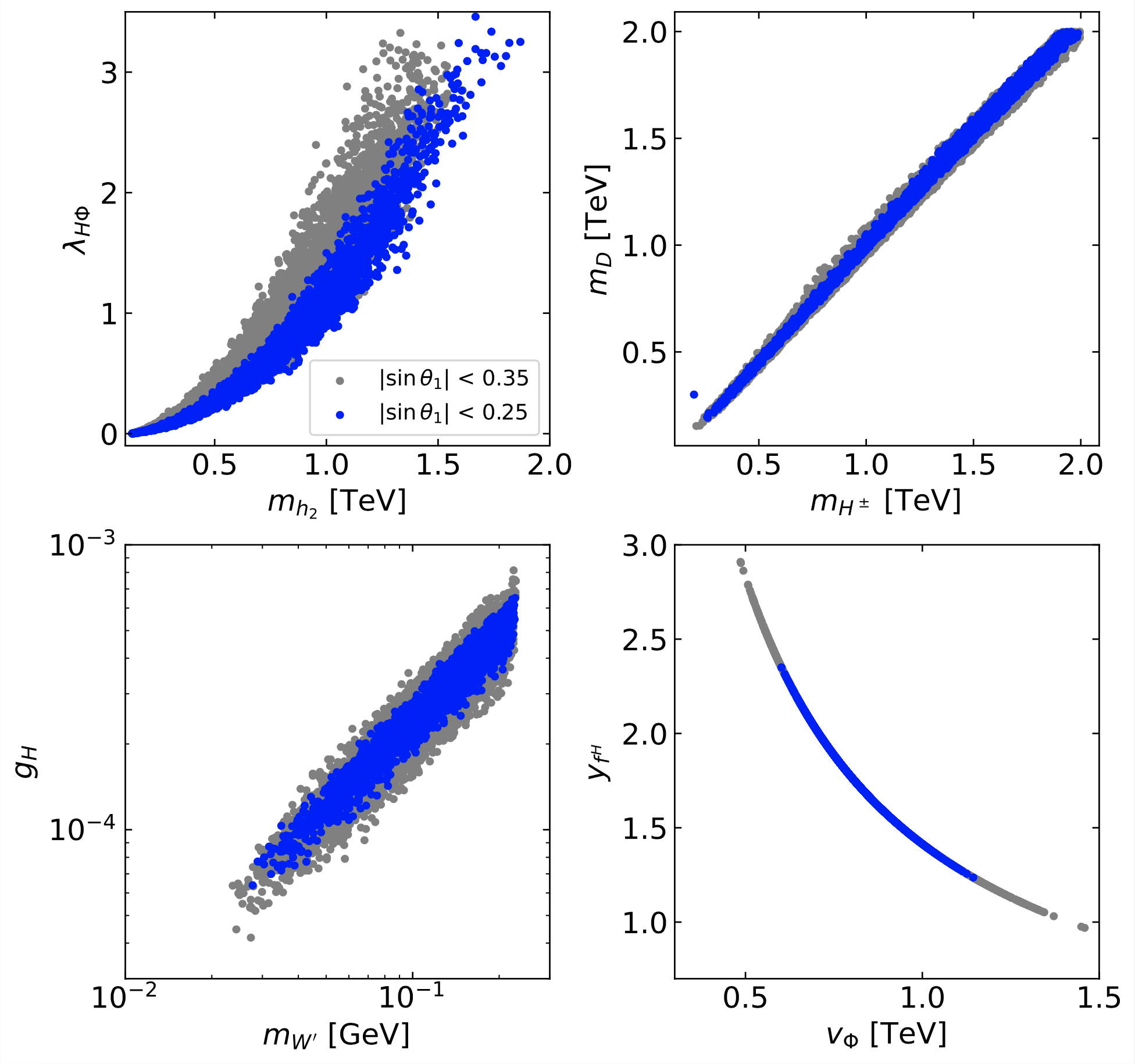
Given the viable model parameter space, we find that the FOPT is most likely to occur in the second step of a two-step phase transition, as sketched in the right panel of Fig. 1 where , and . The parameter space conducive to this two-step phase transition is depicted in Fig. 4 with different choices of the constraint on the mixing angle . The gray area denotes , a constraint derived from Higgs signal strength data measured at the CMS experiment, while the blue area indicates , a requirement based on the combined Higgs signal strength data from both the ATLAS and CMS experiments. We observe that imposing a stringent constraint on leads to a significant reduction in the viable parameter space necessary to achieve the two-step phase transition. Specifically, upon comparing the gray and blue regions in Fig. 4, a tighter constraint on requires a smaller value for and a narrower region on the and planes. Additionally, it results in stronger upper and lower bounds on .
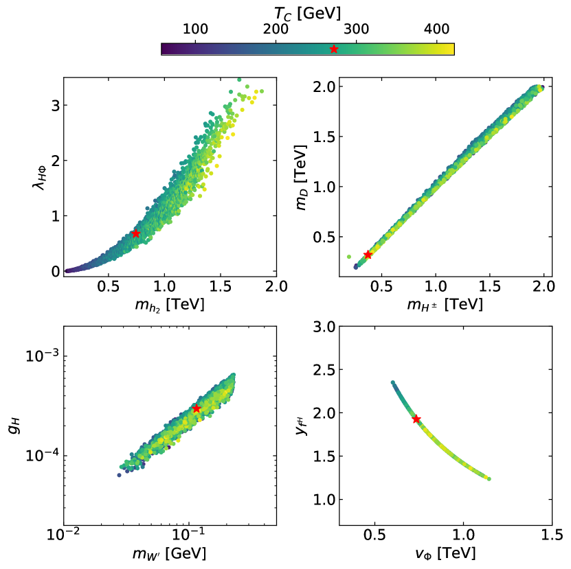
In Fig. 5, we showcase results for . The color within this figure indicates the strength of the EWPT in the second step, denoted here by 333Not to be confused with the gauge fixing parameter having the same symbol discussed in Appendix D., where , which remains gauge invariant under the high-T treatment of the effective scalar potential. If one takes a glimpse back at the left panel of Fig. 3, is the intersection point between the purple and dash-dotted lines. A commonly accepted criterion to avoid the washout of baryon number generated during the phase transition is Patel and Ramsey-Musolf (2011). We find that in our scanning region. Similar to Fig. 5, Fig. 6 show the viable parameter region, but with the color indicating the critical temperature . Interestingly, lies within the electroweak scale.
As shown in the top-left panel of Fig. 5, for a fixed value of , an increase in the quadratic coupling leads to a larger and therefore a stronger phase transition. This occurs due to the presence of a tree-level barrier, the height of which is proportional to , in the second step of the phase transition. This effect has been extensively studied in SM extensions involving gauge singlets Profumo et al. (2007); Espinosa et al. (2012a); Curtin et al. (2014); Chiang et al. (2018) and real triplets Patel and Ramsey-Musolf (2013); Blinov et al. (2015); Niemi et al. (2021b). Additionally, an increase in also results in a lower critical temperature, as shown in the top-left panel of Fig. 6.
In the top-right panel of Fig. 5 or 6, the viable parameter space projected on the plane shows a distinct shape, which is due to the recent precision measurement of the boson mass by the CDF-II collaboration Tran et al. (2023)444If one instead uses the data from the PDG Zyla et al. (2020b), excluding the CDF-II measurement, the most significant change in the parameter space is the mass splitting between the charged Higgs and the dark Higgs. The PDG data favor a smaller mass splitting Tran et al. (2023).. Furthermore, this panel indicates that the dark Higgs and charged Higgs must satisfy lower bounds of GeV and GeV, respectively.
We observe that in this model, even for scalar masses on the order of 1 TeV, the two-step phase transition can occur, which contrasts with the generic upper bound of GeV as discussed in Ref. Ramsey-Musolf (2020). This larger range for the new scalar masses arises because the extra scalar boson considered in Ref. Ramsey-Musolf (2020) obtains its mass solely from the SM doublet VEV , whereas the inert Higgs doublet in G2HDM is also a member of a doublet under a hidden that is broken by a new VEV , thereby generating additional contributions to their masses. For example, two-step transition requires and thus
| (47) |
where () is the critical temperature for the first (second) step and is the electroweak temperature. Assuming a small mixing between -parity odd scalar fields, one can obtain the dark Higgs boson mass at zero temperature as
| (48) | |||||
| (49) |
Taking numerical values of , , , , and , we obtain
| (50) |
With GeV and TeV, one can get an upper bound of TeV.
The mass of the DM particle, , falls in the sub-GeV range of 0.02 GeV to 0.25 GeV, as revealed in the bottom-left panel of Fig. 5 or 6. This restriction range of is due to the limits on the new gauge coupling , which arises from dark photon searches Ramos et al. (2021b, a); Tran et al. (2023), as well as the bounds on . As shown in the bottom-right panel of Fig. 5 or 6, falls within the range of . This range represents a combination of collider constraints illustrated in Fig. 2 and the two-step phase transition condition requirement for , as shown in the top-left panel of Fig. 5 or 6. With the mass of the heavy hidden fermions fixed at 1 TeV, a relatively large value of the Yukawa coupling is required in the small region of . Nevertheless is still below allowed by perturbative unitarity arguments. Additionally, smaller regions of show a trend towards larger values of . Finally, the bottom-right panel of Fig. 6 shows that increases in regions of larger values of .
IV Stochastic Gravitational Waves
During a cosmological FOEWPT, the production of GWs is a result of several distinct mechanisms. In particular, primary sources of GW generation are bubble collisions, sound waves, and magneto-hydrodynamic (MHD) turbulence Caprini et al. (2016); Weir (2018). For bubble collisions, the GW is generated from the stress energy localized at the bubble wall. Such GW spectra have been estimated analytically Jinno and Takimoto (2017) and numerically under the so-called thin-wall and envelope approximations respectively Kosowsky et al. (1992a, b); Kosowsky and Turner (1993); Huber and Konstandin (2008b). On the other hand, the motion of the fluid in the plasma during the phase transition generates sound waves. As the sound waves dissipate, they transfer energy into GWs Hindmarsh et al. (2014); Giblin and Mertens (2013, 2014); Hindmarsh et al. (2015). The GW spectrum from this source typically relies on large scale lattice simulations Hindmarsh et al. (2014, 2015, 2017); Cutting et al. (2020). However, an analytical modeling can reproduce the spectra from simulations reasonably well based on the sound shell model Hindmarsh (2018); Hindmarsh and Hijazi (2019). Turbulence can also be induced in the plasma by percolation, particularly MHD turbulence, given that the plasma is fully ionized. This also leads to the production of GWs Caprini and Durrer (2006); Kahniashvili et al. (2008a, b, 2010); Caprini et al. (2009). The significance of each contribution to GW generation is heavily influenced by the characteristics and dynamics of the phase transition. The velocity of the bubble wall is a critical factor in this regard. If the wall velocity is slow, the thermal bath can effectively absorb the energy released during the phase transition, leading to suppression of the GW spectrum. On the other hand, if the bubble wall velocity is relativistic, a considerable amount of energy can be converted into bulk motion. In this study we consider a so-called non-runaway bubbles in which the bubble expansion in the plasma can result in the attainment of a relativistic terminal velocity Caprini et al. (2016). In this case, the contributions from the sound waves and the MHD turbulence are dominant. For recent reviews on GW signals and cosmological first order phase transitions, we refer our readers to Hindmarsh et al. (2021); Athron et al. (2024).
In order to calculate the GW signals resulting from the FOEWPT, the following 4 parameters must be determined: the nucleation temperature, ; the fraction of energy released from the phase transition to the total radiation energy density at the nucleation temperature, ; the inverse duration of the phase transition (usually normalized by , the Hubble rate at the percolation temperature); and the velocity of the bubble wall, . The wall velocity can be calculated from micro-dynamics of particle interactions with the Higgs condensate, its precise value remains undetermined due to the theoretical uncertainties in the calculations. Here we choose in our analysis. The sensitivity of GW detectors can significantly depend on values of bubble wall velocity Friedrich et al. (2022). Within the viable parameter space in G2HDM, we find that sensitivity of LISA detector is maximized around . Higher values of slightly reduce sensitivity, while it drops dramatically for smaller ().
The nucleation temperature is usually determined by solving the following equation
| (51) |
where is the tunneling probability per unit time per unit volume, which is calculated using the following formula
| (52) |
Here represents the three-dimensional Euclidean action corresponding to the critical bubble, which is given by
| (53) |
where denotes a collection of classical scalar fields 555In the present context, . that minimizes the action and are determined by solving the following equation of motion
| (54) |
with the boundary conditions
| (55) |
Here we utilize the CosmoTransitions package Wainwright (2012) to numerically solve the bounce equation in Eq. (54) and subsequently calculate the action. A rough estimation of the nucleation temperature, , can be obtained by solving the following nucleation condition
| (56) |
The inverse duration parameter can be calculated using the following equation
| (57) |
where is the temperature at which GWs are generated and it is expected that , and is the Hubble rate at . The parameter can be obtained by
| (58) |
where is the vacuum energy density, is the total radiation energy density with being the number of relativistic degrees of freedom at , and is the difference in scalar potential between the lower and higher phases.
With these portal parameters, we utilize the PTPlot package Hindmarsh et al. (2017); Caprini et al. (2020) to calculate the GW spectrum. To quantify the detectability of the signals, one can define the signal-to-noise ratio (SNR) Caprini et al. (2020)
| (59) |
where is the duration of the observation period in years, represents the GW energy fraction spectrum from the FOEWPT and is the sensitivity of the experimental setup. It is commonly accepted that a SNR value of 10 is the threshold for detection. For the benchmark point BM depicted in Fig. 3, the values of , , and LISA SNR we obtained are GeV, 0.43, 332 and 144 respectively.
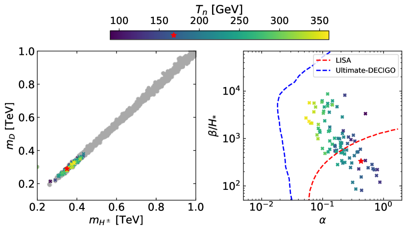
By applying the nucleation condition described in Eq. (56) to the two-step phase transition data points, we find that only approximately of the data points meet this criterion. While the range of other parameters remains largely unchanged after applying the nucleation condition, the upper bound on the masses of the charged Higgs and dark Higgs is significantly altered. In particular, as shown in the left panel of Fig. 7, it is required that GeV and GeV. Additionally, as shown in the same panel, we can see that the value of the nucleation temperature tends to increase in the regions of larger masses of the charged Higgs and dark Higgs.
The right panel of Fig. 7 shows the surviving points on the () plane after applying the nucleation condition. As a result, the range of is approximately () and the range of is approximately (). All prediction points lie within the sensitivity range of the Ultimate-DECIGO detector (dashed blue line) Kawamura et al. (2011) and a part of them lies within the LISA sensitivity region with a SNR > 10 Caprini et al. (2020) 666Here, in order to obtain the Ultimate-DECIGO and LISA sensitivity lines, we take = 100 GeV and for the purpose of illustration.. A larger value of suggests more energy from the plasma being converted into GWs, while a smaller value of implies a longer duration of the strong first-order phase transition, thus leading to an enhancement of the GW energy spectrum.
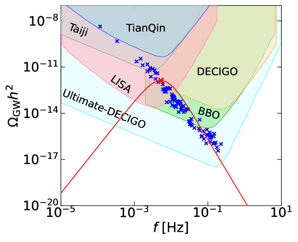
The predicted energy spectrum peaks of GWs as a function of frequency are presented in Fig. 8. As a result, the generated GWs resulting from the FOEWPT in the two-step transition have peak frequencies within the range of Hz and peak yields vary in the range . These peak yields are expected to be accessible at BBO, LISA, (Ultimate-)DECIGO, TianQin and Taiji detectors in the future. For demonstration purposes, we show the GW spectrum generated from the benchmark point BM as the solid red line in Fig. 8. The benchmark point is selected with a relatively high value of in order to increase the magnitude of the generated GWs, making it possible to be accessible by BBO, LISA, and (Ultimate-)DECIGO.
V Dark Matter Direct Detection Prospects
In recent decades, significant advancements have been made in the design and construction of direct-detection experiments aimed at detecting weakly interacting massive particles (WIMPs) that are potential candidates for DM. Notable examples of these experiments include CRESST III Angloher et al. (2017), DarkSide-50 Agnes et al. (2018, 2023), XENON1T Aprile et al. (2018, 2019), PandaX-4T Meng et al. (2021), and LZ Aalbers et al. (2023). These experiments have led to significant improvements in searches for few keV-scale nuclear recoils, which are indicative of spin-independent scattering of WIMPs with masses greater than GeV. While the next generation of experiments, such as PandaX30T Wang et al. (2023b), XENONnT Aprile et al. (2020), DarkSide-20k Aalseth et al. (2018), and DARWIN Aalbers et al. (2016), are expected to explore a large fraction of the theoretically well-motivated parameter space for this mass range and even reach the neutrino fog, there is growing interest in exploring DM with sub-GeV mass ranges Essig et al. (2022).
However, the detection of sub-GeV DM remains challenging due to the low nuclear recoil energies involved and the finite detector thresholds. Nevertheless, new technologies capable of achieving lower detector energy thresholds, down to meVeV scales, are being proposed Essig et al. (2022). For example, the HeRALD proposal Hertel et al. (2019) involves an array of microchannel plates and photomultiplier tubes that can measure ionization signals resulting from DM interactions with helium nuclei. This approach enables HeRALD to reach energy thresholds as low as a few meV, thus making it suitable for probing DM in the sub-GeV mass region.
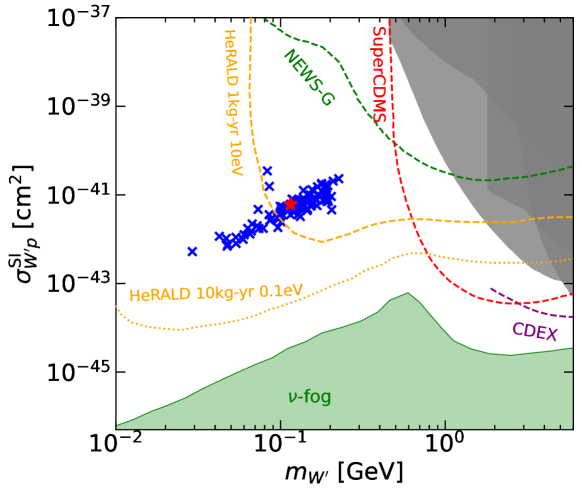
As demonstrated before, a two-step transition for achieving a strong FOEWPT in the G2HDM leads to the prediction that the DM mass falls within the sub-GeV range. This prediction renders the DM candidate a suitable candidate for exploration in upcoming DM direct detection experiments. Fig. 9 shows the spin-independent DM-proton scattering cross-section as a function of DM mass for the parameter space being probed by gravitational wave detectors. While NEWS-G Durnford and Piro (2021), SuperCDMS Agnese et al. (2017), and CDEX Ma et al. (2020) are designed to probe DM with masses around and above GeV, HeRALD with 1 kg-year of exposure and 10 eV of detector energy threshold can probe part of our parameter space that predicts gravitational wave signals. HeRALD can fully cover our parameter space with 10 kg-year of exposure and a detector energy threshold of 0.1 eV. Therefore, it highlights an interesting interplay between future DM direct detection and GW signal searches.
VI Conclusions
We investigate the electroweak phase transition and the possibility of detecting GW signals resulting from the phase transition in the simplified G2HDM. The simplified G2HDM is a well-motivated dark matter model with a hidden non-abelian gauge boson serving as a DM candidate. The stability of the DM candidate is protected by an accidental -parity in the model. We take into account both theoretical and experimental constraints, with the latter including Higgs experimental data, electroweak precision measurements, dark photon and DM direct search experiments.
We derive the effective potential in the simplified G2HDM, including the one-loop finite temperature correction with daisy resummation. The effective potential consists of three background fields (, , ) that give rise to rich patterns of phase transition. We require at zero temperature to anti-restore the -parity and analyze the possible first-order electroweak phase transition in the early universe.
We identify several rather distinctive features of the simplified G2HDM as follows:
-
•
A two-step phase transition pattern is possible, where the symmetric phase transfers to the inert doublet direction first and subsequently to the electroweak vacuum phase with a non-zero hidden doublet VEV in addition to the SM doublet VEV as the temperature decreases. Using the high-T approximation in the effective potential that manifests gauge invariance, we found that the former transition is a second-order phase transition, while the latter can be first-order due to a tree-level barrier. The first step breaks -parity and the second step restores it.
-
•
Unlike the conventional symmetry model, where the two-step FOEWPT imposes strict upper bounds on new scalar masses, these bounds can be relaxed in G2HDM. In G2HDM, the new scalars receive contributions to their masses from a hidden sector VEV, allowing for somewhat larger BSM scalar masses to be compatible with a FOEWPT. However, due to the perturbative limit on the couplings and the bubble nucleation condition for GWs, scalar masses can only reach (1 TeV). In particular, the extra -parity even scalar boson mass can reach 1.8 TeV, the -parity odd scalars and can only reach up to 500 GeV. Our findings also suggest that the Higgs portal coupling needs to be sizable and the VEV of the singlet/ doublet scalar needs to be within the range of 0.5 TeV to 1.4 TeV.
-
•
The predicted GW energy spectrum from two-step FOEWPT in this model can be probed in the next-generation GW detectors. In particular, we find that the peak frequencies lie within the range of Hz, and the peak yields vary from to . These frequencies and yields can be covered by BBO, LISA, (Ultimate-)DECIGO, TianQin, and Taiji in the future.
-
•
Interestingly, these GW probed regions can also be searched for in the future dark matter direct detection experiments, such as the superfluid-He target detectors. While it is possible for the DM candidate to be heavy Tran et al. (2023), we have concentrated on the light mass region due to its potential accessibility by future direct detection experiments.
-
•
Albeit the above distinctive features are obtained here in a specific model of G2HDM, it is conceivable that they might be present in other class of models, for instance in certain limit of the IHDM, augmented further by a scalar singlet. After all, the scalar potential of G2HDM can be regarded as a gauged version of the one from IHDM, supplemented by a hidden doublet which is nevertheless a SM singlet.
Finally, we note that the results in this work are presented at leading order, i.e., using the high-T approximation in the effective potential. Higher-order corrections that include both a systematical thermal resummation and a properly gauge-invariant treatment are needed to be taken into account to obtain more accurate predictions. This can be done by using the state-of-the-art dimensional reduction method reducing the simplified G2HDM to a 3d effective field theory. To fully resolve the IR problem and properly identify the boundary between FOEWPT-viable and crossover regions of the parameter space, lattice studies are required. We will defer this exploration to the future.
Acknowledgments
We would like to thank Eibun Senaha for useful discussions. This work was supported in part by the National Natural Science Foundation of China, grant Nos. 19Z103010239, 12350410369 (VQT) and 11975150, 12375094 (MJRM) and the NSTC of Taiwan, grant Nos. 111-2112-M-001-035, 113-2112-M-001-001 (TCY) and 112-2811-M-001-089 (VQT). VQT would like to thank the Medium and High Energy Physics Group at the Institute of Physics, Academia Sinica, Taiwan for their hospitality during the course of this work.
Appendix A Field Dependent Masses
We will work in the Landau gauge where all the Goldstone bosons are massless and the ghost contributions can be ignored. The thermal mass corrections for the scalar fields (, and ) and the longitudinal components of the gauge fields ( and ) are also included in this work for the daisy resummation. These thermal mass corrections are given in Appendix B.
A.1 Gauge Bosons
In what follows, we will suppress the temperature dependence of the constant background fields and and denote them simply as and unless stated otherwise. For convenience, we define the following combinations of the background fields
| (60) | |||||
| (61) |
There is only one electric charged vector boson, the SM , with field dependent mass given by
| (62) | |||||
| (63) |
In general, doesn’t mix with other gauge fields and its field dependent mass is given by
| (64) | |||||
| (65) |
All the other 5 gauge bosons associated with the remaining 5 generators in G2HDM are electrically neutral and in general mixed together. In the basis of , one finds the transverse mass matrix
It is clear that for , can mix with , and . Thus in general and have different masses and do not combine into two complex conjugate fields (denoted by in previous studies) unless one of the and or both vanishes! Note that we have included a Stueckelberg mass for the while for the we set its Stueckelberg mass to be zero due to phenomenological reasons discussed in earlier works. We also do not include kinetic mixing among the two s.
Despite its unappealing look, the determinant of Eq. (A.1) vanishes for arbitrary values of , and , all of which can be different from their vacuum values of , and respectively at zero temperature. So it has at least one zero eigenvalue which can be identified as the photon 777Including a Stueckelberg mass for the hypercharge gauge field would break this statement.. The exact results of the eigenvalues of depend on the detailed symmetry breaking patterns. We will denote the eigenstates of Eq. (A.1) as the transverse and with eigenvalues and for , and 4 respectively.
For the longitudinal components of the neutral gauge bosons, we have to include their thermal masses as well. The mass matrix now becomes
| (67) |
We will denote the eigenstates of in (67) as the longitudinal and with eigenvalues and for and 4 respectively.
Setting all the thermal masses to be zeros, , and in the above formulae, one can reproduce the tree level mass spectrum and mixings for the neutral gauge bosons presented in Sec. II.2 for the zero temperature case. For instance, and will have the same mass and can combine into two complex fields which will be considered as sub-GeV DM candidate in this work.
A.2 Scalar Bosons
In G2HDM, the charged scalar and in (3) mix according to the following mass matrix
| (68) |
Here we have defined . Note that depends on the values of , its eigenvalues also depend on the detail of the symmetry breaking patterns. Including the thermal mass corrections, we have
| (69) |
We will denote the two eigenstates as and and their corresponding eigenvalues of () are and ( and ) respectively. Explicitly, we have
with and is given by (A.2) with set to .
In the general spontaneous symmetry breaking in G2HDM, all the other scalar fields in the three doublets mix together according to their CP properties. This is expected since the parameters in the scalar potential of G2HDM are all real and the scalar potential is CP conserving. The real and imaginary fields have opposite CP properties and they should not mix!
For the CP-even scalars in the basis of , the mass matrix is given by
| (71) |
with the diagonal elements defined as follows
| (72) | |||||
| (73) | |||||
| (74) | |||||
| (75) |
Including the thermal masses, we have
| (76) |
We denote the eigenvalues of and as and respectively for the CP-even states with and .
For the CP-odd scalars in the basis , the mass matrix is
| (77) |
with the following diagonal elements
| (78) | |||||
| (79) | |||||
| (80) | |||||
| (81) |
Similarly, including the thermal masses, we have
| (82) |
We denote the eigenvalues of and as and respectively for the CP-odd states with and .
Since the matrix elements of and depend on the values of and , the scalar mass spectrum depends on the detail of the symmetry breaking patterns just like the gauge bosons. Similarly one can reproduce the zero temperature mass spectra and mixings for the scalars presented in Sec. II.2 by ignoring the thermal masses and setting , and in the above formulae. For example, and will have the same mass and they can be combined into two complex Goldstone bosons absorbed by the longitudinal components of , and and can be combined into and , and so on.
A.3 Fermions
The gauge invariant Yukawa couplings in G2HDM lead to the following fermionic mass terms in the Lagrangian Huang et al. (2016a)
| (83) | |||||
Since the lower left blocks in the mass matrices vanish, the SM fermions will not mix with the hidden fermions in G2HDM even if . The Yukawa matrices and can be blocked diagonalized independently. Since fermion loops do not suffer from the infrared problems associated with the zero Matsubara frequencies in the bosonic case, daisy resummation is not necessary. The leading temperature effects for the fermion masses are usually captured via the following prescriptions
| (84) | |||||
| (85) |
where and are the eigenvalues of the Yukawa matrices (or ) and (or ) respectively. The temperature dependence for the fermion masses are coming through the classical fields and only. For simplicity, we will consider just the heavy top quark and its hidden heavy partner from the third generation in the numerical work since they represent the most dominant contribution from the fermion sector.
Appendix B Thermal Masses
In this appendix, we list the thermal mass (Debye screening mass) for all the scalar and vector bosons in G2HDM. Including these masses are essential for the resummation of the daisy diagrams in the finite temperature effective potential.
For the two doublets and , using the field components defined in Eq. (3), we found
| (87) | |||||
and for the hidden doublet , using Eq. (4), we got
| (88) | |||||
For the Yukawa couplings, we will keep only the contributions from the SM top quark () and its heavy partner () in G2HDM.
For the SM gauge bosons, we have
| (89) | |||||
| (90) |
For the hidden gauge bosons, we have
| (91) | |||||
| (92) |
In the thermal masses of the gauge bosons, we have summed over all three generations of quarks and leptons in G2HDM.
Appendix C Thermal Integrals
The definition of depends on whether is a boson or a fermion , i.e.
| (93) |
Note that in our notation, . In the literature, some authors’ is our .
For high-T where , one has the following series expansions Quiros (1999)
| (94) | ||||
| (95) |
where , , and and are the Euler -function and Riemann -function respectively. Numerically, we have
| (96) | ||||
Note that there is no term in ! For high-T, keeping the first lines in (C) and (C) are usually sufficient!
On the other hand, we also have the following series representations Anderson and Hall (1992)
| (97) | ||||
| (98) |
where is the modified Bessel function of second kind which falls off exponentially for large positive values of . For high mass or low temperature where , these series representations converge rapidly. Usually, taking the first five terms in the series is sufficient Bernon et al. (2018); Fabian et al. (2021).
The thermal integral in (33) is defined by Arnold and Espinosa (1993); Carrington (1992)
| (99) |
Note that for the scalars and longitudinal components of the gauge bosons we have included the resummation effects from the daisy (ring) diagrams from higher loops in the thermal corrections. and are the field dependent masses (mass eigenvalues in case of mixings) with and without the thermal mass correction respectively for particle .
It has been shown recently Curtin et al. (2018) that at high-T the daisy resummation can be quite poor for large values of the quartic coupling in BSM and does not shown how decoupling occurs when the internal mass of the BSM particle is large compared with the temperature. More accurate calculation would have to include the superdaisy diagrams which will lead one to solve the gap equations Curtin et al. (2018). We will not get into this business here. Also ignored here is the two-loop corrections to the finite temperature effective potential which have been shown quite relevant to determine the strength of the phase transition in MSSM Espinosa (1996).
Appendix D Gauge-Invariant Method Beyond Leading Order and Scale Dependence
The determination of the phase transition quantities such as and in a gauge theory can lead to the gauge fixing parameter dependence if the effective potential is calculated beyond the leading high-T approximation. However one can treat the gauge dependence issue using the -expansion method proposed in Ref.Patel and Ramsey-Musolf (2011). Such method is based on the Nielsen-Fukuda-Kugo (NFK) identity Nielsen (1975); Fukuda and Kugo (1976), which states that the energies at the stationary points of the effective potential are independent of the gauge fixing parameter . The NFK identity can be described by
| (100) |
where the functional can be found explicitly in Ref. Nielsen (1975).
By expanding both the effective potential and the functional in powers of ,
| (101) | ||||
| (102) |
and, for example, considering the first order with respect to , one can obtain from (100)
| (103) |
which implies that the -dependence of can be eliminated at the extremal points of the tree-level potential. Therefore, the critical temperature to can be determined by evaluating the degeneracy condition of the effective potential at the stationary points of the tree-level potential. For the transition from the phase to phase in G2HDM as depicted in the right panel of Fig. 1 where , and , the critical temperature can be determined by solving the following equation
| (104) |
where and are the extremal points at the tree-level potential. On the other hand, the value of is determined by utilizing the high-T expansion effective potential.
Another issue that arises in the calculation beyond the high-T expansion effective potential is the dependence on the renormalization scale in the Coleman-Weinberg effective potential . This dependence can have a significant impact on the properties of phase transitions and the associated predicted GW signals Croon et al. (2021); Gould and Tenkanen (2021). To mitigate this dependence, renormalization group (RG) improvement can be applied to the effective potential Kastening (1992); Bando et al. (1993); Ford et al. (1993); Funakubo and Senaha (2024a, b). This can be done by running the parameters in the tree-level effective potential using the functions given in Appendix F. At leading order, the RG improved potential satisfies
| (105) |
which ensures independence from the choice of .
Appendix E The Critical Temperatures
In this section, we show the analytical expressions for the critical temperatures in the two-step phase transition. The critical temperature for the first step [] can be easily obtained by solving the degenerate condition . This gives the result of
| (106) |
where fixed by the tree level tadpole condition and is given by (39).
For the second step , by solving the following degenerate condition
| (107) |
one obtains
| (108) |
where
| (109) | |||||
| (110) |
We note that with the viable parameter space in the model, the critical temperature stays in the electroweak scale as shown in Fig. 6.
Appendix F Renormalization Group Equations
Here we present the one loop renormalization group equations in G2HDM. The -function, computed with the help of SARAH Staub (2014), is defined as , where denotes a generic coupling/mass and is the renormalization scale.
Gauge couplings:
| (111) | |||||
| (112) | |||||
| (113) | |||||
| (114) | |||||
| (115) |
Scalar masses and quartic couplings:
| (116) | |||||
| (117) | |||||
| (118) | |||||
| (119) | |||||
| (120) | |||||
| (121) | |||||
| (122) | |||||
Yukawa couplings:
| (123) | |||||
| (124) |
References
- Kajantie et al. (1996a) K. Kajantie, M. Laine, K. Rummukainen, and M. E. Shaposhnikov, Phys. Rev. Lett. 77, 2887 (1996a), arXiv:hep-ph/9605288 .
- Rummukainen et al. (1998) K. Rummukainen, M. Tsypin, K. Kajantie, M. Laine, and M. E. Shaposhnikov, Nucl. Phys. B 532, 283 (1998), arXiv:hep-lat/9805013 .
- Laine and Rummukainen (1999) M. Laine and K. Rummukainen, Nucl. Phys. B Proc. Suppl. 73, 180 (1999), arXiv:hep-lat/9809045 .
- Aoki et al. (1999) Y. Aoki, F. Csikor, Z. Fodor, and A. Ukawa, Phys. Rev. D 60, 013001 (1999), arXiv:hep-lat/9901021 .
- McDonald (1994) J. McDonald, Phys. Lett. B 323, 339 (1994).
- Profumo et al. (2007) S. Profumo, M. J. Ramsey-Musolf, and G. Shaughnessy, JHEP 08, 010 (2007), arXiv:0705.2425 [hep-ph] .
- Cline et al. (2009) J. M. Cline, G. Laporte, H. Yamashita, and S. Kraml, JHEP 07, 040 (2009), arXiv:0905.2559 [hep-ph] .
- Espinosa et al. (2012a) J. R. Espinosa, T. Konstandin, and F. Riva, Nucl. Phys. B 854, 592 (2012a), arXiv:1107.5441 [hep-ph] .
- Cline and Kainulainen (2013a) J. M. Cline and K. Kainulainen, JCAP 01, 012 (2013a), arXiv:1210.4196 [hep-ph] .
- Alanne et al. (2014) T. Alanne, K. Tuominen, and V. Vaskonen, Nucl. Phys. B 889, 692 (2014), arXiv:1407.0688 [hep-ph] .
- Curtin et al. (2014) D. Curtin, P. Meade, and C.-T. Yu, JHEP 11, 127 (2014), arXiv:1409.0005 [hep-ph] .
- Profumo et al. (2015) S. Profumo, M. J. Ramsey-Musolf, C. L. Wainwright, and P. Winslow, Phys. Rev. D 91, 035018 (2015), arXiv:1407.5342 [hep-ph] .
- Huang and Li (2015) F. P. Huang and C. S. Li, Phys. Rev. D 92, 075014 (2015), arXiv:1507.08168 [hep-ph] .
- Kotwal et al. (2016) A. V. Kotwal, M. J. Ramsey-Musolf, J. M. No, and P. Winslow, Phys. Rev. D 94, 035022 (2016), arXiv:1605.06123 [hep-ph] .
- Vaskonen (2017) V. Vaskonen, Phys. Rev. D 95, 123515 (2017), arXiv:1611.02073 [hep-ph] .
- Ghorbani (2017) P. H. Ghorbani, JHEP 08, 058 (2017), arXiv:1703.06506 [hep-ph] .
- Cline et al. (2017) J. M. Cline, K. Kainulainen, and D. Tucker-Smith, Phys. Rev. D 95, 115006 (2017), arXiv:1702.08909 [hep-ph] .
- Beniwal et al. (2017) A. Beniwal, M. Lewicki, J. D. Wells, M. White, and A. G. Williams, JHEP 08, 108 (2017), arXiv:1702.06124 [hep-ph] .
- Kurup and Perelstein (2017) G. Kurup and M. Perelstein, Phys. Rev. D 96, 015036 (2017), arXiv:1704.03381 [hep-ph] .
- Chiang et al. (2018) C.-W. Chiang, M. J. Ramsey-Musolf, and E. Senaha, Phys. Rev. D 97, 015005 (2018), arXiv:1707.09960 [hep-ph] .
- Carena et al. (2019) M. Carena, M. Quirós, and Y. Zhang, Phys. Rev. Lett. 122, 201802 (2019), arXiv:1811.09719 [hep-ph] .
- Carena et al. (2018) M. Carena, Z. Liu, and M. Riembau, Phys. Rev. D 97, 095032 (2018), arXiv:1801.00794 [hep-ph] .
- Grzadkowski and Huang (2018) B. Grzadkowski and D. Huang, JHEP 08, 135 (2018), arXiv:1807.06987 [hep-ph] .
- Huang et al. (2018a) F. P. Huang, Z. Qian, and M. Zhang, Phys. Rev. D 98, 015014 (2018a), arXiv:1804.06813 [hep-ph] .
- Alves et al. (2019) A. Alves, T. Ghosh, H.-K. Guo, K. Sinha, and D. Vagie, JHEP 04, 052 (2019), arXiv:1812.09333 [hep-ph] .
- Ghorbani and Ghorbani (2020) K. Ghorbani and P. H. Ghorbani, J. Phys. G 47, 015201 (2020), arXiv:1804.05798 [hep-ph] .
- Cheng and Bian (2018) W. Cheng and L. Bian, Phys. Rev. D 98, 023524 (2018), arXiv:1801.00662 [hep-ph] .
- Alanne et al. (2020) T. Alanne, T. Hugle, M. Platscher, and K. Schmitz, JHEP 03, 004 (2020), arXiv:1909.11356 [hep-ph] .
- Gould et al. (2019) O. Gould, J. Kozaczuk, L. Niemi, M. J. Ramsey-Musolf, T. V. I. Tenkanen, and D. J. Weir, Phys. Rev. D 100, 115024 (2019), arXiv:1903.11604 [hep-ph] .
- Carena et al. (2020) M. Carena, Z. Liu, and Y. Wang, JHEP 08, 107 (2020), arXiv:1911.10206 [hep-ph] .
- Li et al. (2019) H.-L. Li, M. Ramsey-Musolf, and S. Willocq, Phys. Rev. D 100, 075035 (2019), arXiv:1906.05289 [hep-ph] .
- Bell et al. (2019) N. F. Bell, M. J. Dolan, L. S. Friedrich, M. J. Ramsey-Musolf, and R. R. Volkas, JHEP 09, 012 (2019), arXiv:1903.11255 [hep-ph] .
- Inoue et al. (2016) S. Inoue, G. Ovanesyan, and M. J. Ramsey-Musolf, Phys. Rev. D 93, 015013 (2016), arXiv:1508.05404 [hep-ph] .
- Niemi et al. (2019) L. Niemi, H. H. Patel, M. J. Ramsey-Musolf, T. V. I. Tenkanen, and D. J. Weir, Phys. Rev. D 100, 035002 (2019), arXiv:1802.10500 [hep-ph] .
- Chala et al. (2019) M. Chala, M. Ramos, and M. Spannowsky, Eur. Phys. J. C 79, 156 (2019), arXiv:1812.01901 [hep-ph] .
- Zhou et al. (2019) R. Zhou, W. Cheng, X. Deng, L. Bian, and Y. Wu, JHEP 01, 216 (2019), arXiv:1812.06217 [hep-ph] .
- Bochkarev et al. (1990) A. I. Bochkarev, S. V. Kuzmin, and M. E. Shaposhnikov, Phys. Lett. B 244, 275 (1990).
- McLerran et al. (1991) L. D. McLerran, M. E. Shaposhnikov, N. Turok, and M. B. Voloshin, Phys. Lett. B 256, 451 (1991).
- Bochkarev et al. (1991) A. I. Bochkarev, S. V. Kuzmin, and M. E. Shaposhnikov, Phys. Rev. D 43, 369 (1991).
- Turok and Zadrozny (1991) N. Turok and J. Zadrozny, Nucl. Phys. B 358, 471 (1991).
- Cohen et al. (1991) A. G. Cohen, D. B. Kaplan, and A. E. Nelson, Phys. Lett. B 263, 86 (1991).
- Turok and Zadrozny (1992) N. Turok and J. Zadrozny, Nucl. Phys. B 369, 729 (1992).
- Nelson et al. (1992) A. E. Nelson, D. B. Kaplan, and A. G. Cohen, Nucl. Phys. B 373, 453 (1992).
- Funakubo et al. (1994) K. Funakubo, A. Kakuto, and K. Takenaga, Prog. Theor. Phys. 91, 341 (1994), arXiv:hep-ph/9310267 .
- Davies et al. (1994) A. T. Davies, C. D. froggatt, G. Jenkins, and R. G. Moorhouse, Phys. Lett. B 336, 464 (1994).
- Cline et al. (1996) J. M. Cline, K. Kainulainen, and A. P. Vischer, Phys. Rev. D 54, 2451 (1996), arXiv:hep-ph/9506284 .
- Funakubo et al. (1995) K. Funakubo, A. Kakuto, S. Otsuki, K. Takenaga, and F. Toyoda, Prog. Theor. Phys. 94, 845 (1995), arXiv:hep-ph/9507452 .
- Funakubo et al. (1996) K. Funakubo, A. Kakuto, S. Otsuki, and F. Toyoda, Prog. Theor. Phys. 96, 771 (1996), arXiv:hep-ph/9606282 .
- Cline and Lemieux (1997) J. M. Cline and P.-A. Lemieux, Phys. Rev. D 55, 3873 (1997), arXiv:hep-ph/9609240 .
- Fromme et al. (2006) L. Fromme, S. J. Huber, and M. Seniuch, JHEP 11, 038 (2006), arXiv:hep-ph/0605242 .
- Cline et al. (2011) J. M. Cline, K. Kainulainen, and M. Trott, JHEP 11, 089 (2011), arXiv:1107.3559 [hep-ph] .
- Dorsch et al. (2013) G. C. Dorsch, S. J. Huber, and J. M. No, JHEP 10, 029 (2013), arXiv:1305.6610 [hep-ph] .
- Cline and Kainulainen (2013b) J. M. Cline and K. Kainulainen, Phys. Rev. D 87, 071701 (2013b), arXiv:1302.2614 [hep-ph] .
- Dorsch et al. (2014) G. C. Dorsch, S. J. Huber, K. Mimasu, and J. M. No, Phys. Rev. Lett. 113, 211802 (2014), arXiv:1405.5537 [hep-ph] .
- Fuyuto and Senaha (2015) K. Fuyuto and E. Senaha, Phys. Lett. B 747, 152 (2015), arXiv:1504.04291 [hep-ph] .
- Chao and Ramsey-Musolf (2015) W. Chao and M. J. Ramsey-Musolf, (2015), arXiv:1503.00028 [hep-ph] .
- Fuyuto et al. (2016) K. Fuyuto, J. Hisano, and E. Senaha, Phys. Lett. B 755, 491 (2016), arXiv:1510.04485 [hep-ph] .
- Chiang et al. (2016) C.-W. Chiang, K. Fuyuto, and E. Senaha, Phys. Lett. B 762, 315 (2016), arXiv:1607.07316 [hep-ph] .
- Haarr et al. (2016) A. Haarr, A. Kvellestad, and T. C. Petersen, (2016), arXiv:1611.05757 [hep-ph] .
- Dorsch et al. (2017a) G. C. Dorsch, S. J. Huber, T. Konstandin, and J. M. No, JCAP 05, 052 (2017a), arXiv:1611.05874 [hep-ph] .
- Basler et al. (2017) P. Basler, M. Krause, M. Muhlleitner, J. Wittbrodt, and A. Wlotzka, JHEP 02, 121 (2017), arXiv:1612.04086 [hep-ph] .
- Fuyuto et al. (2018) K. Fuyuto, W.-S. Hou, and E. Senaha, Phys. Lett. B 776, 402 (2018), arXiv:1705.05034 [hep-ph] .
- Dorsch et al. (2017b) G. C. Dorsch, S. J. Huber, K. Mimasu, and J. M. No, JHEP 12, 086 (2017b), arXiv:1705.09186 [hep-ph] .
- Cherchiglia and Nishi (2017) A. L. Cherchiglia and C. C. Nishi, JHEP 11, 106 (2017), arXiv:1707.04595 [hep-ph] .
- Basler et al. (2018) P. Basler, M. Mühlleitner, and J. Wittbrodt, JHEP 03, 061 (2018), arXiv:1711.04097 [hep-ph] .
- Andersen et al. (2018) J. O. Andersen, T. Gorda, A. Helset, L. Niemi, T. V. I. Tenkanen, A. Tranberg, A. Vuorinen, and D. J. Weir, Phys. Rev. Lett. 121, 191802 (2018), arXiv:1711.09849 [hep-ph] .
- Bernon et al. (2018) J. Bernon, L. Bian, and Y. Jiang, JHEP 05, 151 (2018), arXiv:1712.08430 [hep-ph] .
- Huang and Yu (2018) F. P. Huang and J.-H. Yu, Phys. Rev. D 98, 095022 (2018), arXiv:1704.04201 [hep-ph] .
- Gorda et al. (2019) T. Gorda, A. Helset, L. Niemi, T. V. I. Tenkanen, and D. J. Weir, JHEP 02, 081 (2019), arXiv:1802.05056 [hep-ph] .
- Basler and Mühlleitner (2019) P. Basler and M. Mühlleitner, Comput. Phys. Commun. 237, 62 (2019), arXiv:1803.02846 [hep-ph] .
- Modak and Senaha (2019) T. Modak and E. Senaha, Phys. Rev. D 99, 115022 (2019), arXiv:1811.08088 [hep-ph] .
- Wang et al. (2019) L. Wang, J. M. Yang, M. Zhang, and Y. Zhang, Phys. Lett. B 788, 519 (2019), arXiv:1809.05857 [hep-ph] .
- Wang et al. (2020) X. Wang, F. P. Huang, and X. Zhang, Phys. Rev. D 101, 015015 (2020), arXiv:1909.02978 [hep-ph] .
- Kainulainen et al. (2019) K. Kainulainen, V. Keus, L. Niemi, K. Rummukainen, T. V. I. Tenkanen, and V. Vaskonen, JHEP 06, 075 (2019), arXiv:1904.01329 [hep-ph] .
- Paul et al. (2021) A. Paul, U. Mukhopadhyay, and D. Majumdar, JHEP 05, 223 (2021), arXiv:2010.03439 [hep-ph] .
- Su et al. (2021) W. Su, A. G. Williams, and M. Zhang, JHEP 04, 219 (2021), arXiv:2011.04540 [hep-ph] .
- Apreda et al. (2002) R. Apreda, M. Maggiore, A. Nicolis, and A. Riotto, Nucl. Phys. B 631, 342 (2002), arXiv:gr-qc/0107033 .
- Huber et al. (2016) S. J. Huber, T. Konstandin, G. Nardini, and I. Rues, JCAP 03, 036 (2016), arXiv:1512.06357 [hep-ph] .
- Huber and Konstandin (2008a) S. J. Huber and T. Konstandin, JCAP 05, 017 (2008a), arXiv:0709.2091 [hep-ph] .
- Demidov et al. (2018) S. V. Demidov, D. S. Gorbunov, and D. V. Kirpichnikov, Phys. Lett. B 779, 191 (2018), arXiv:1712.00087 [hep-ph] .
- Brdar et al. (2019) V. Brdar, L. Graf, A. J. Helmboldt, and X.-J. Xu, JCAP 12, 027 (2019), arXiv:1909.02018 [hep-ph] .
- Li et al. (2021) M. Li, Q.-S. Yan, Y. Zhang, and Z. Zhao, JHEP 03, 267 (2021), arXiv:2012.13686 [hep-ph] .
- Huang et al. (2020) W.-C. Huang, F. Sannino, and Z.-W. Wang, Phys. Rev. D 102, 095025 (2020), arXiv:2004.02332 [hep-ph] .
- Chiang and Yamada (2014) C.-W. Chiang and T. Yamada, Phys. Lett. B 735, 295 (2014), arXiv:1404.5182 [hep-ph] .
- Phong et al. (2018) V. Q. Phong, N. C. Thao, and H. N. Long, Phys. Rev. D 97, 115008 (2018), arXiv:1511.00579 [hep-ph] .
- Phong et al. (2022) V. Q. Phong, N. C. Thao, and H. N. Long, Eur. Phys. J. C 82, 1005 (2022), arXiv:2107.13823 [hep-ph] .
- Espinosa et al. (2012b) J. R. Espinosa, B. Gripaios, T. Konstandin, and F. Riva, JCAP 01, 012 (2012b), arXiv:1110.2876 [hep-ph] .
- Chala et al. (2016) M. Chala, G. Nardini, and I. Sobolev, Phys. Rev. D 94, 055006 (2016), arXiv:1605.08663 [hep-ph] .
- Bruggisser et al. (2018a) S. Bruggisser, B. Von Harling, O. Matsedonskyi, and G. Servant, Phys. Rev. Lett. 121, 131801 (2018a), arXiv:1803.08546 [hep-ph] .
- Bruggisser et al. (2018b) S. Bruggisser, B. Von Harling, O. Matsedonskyi, and G. Servant, JHEP 12, 099 (2018b), arXiv:1804.07314 [hep-ph] .
- Bian et al. (2019) L. Bian, Y. Wu, and K.-P. Xie, JHEP 12, 028 (2019), arXiv:1909.02014 [hep-ph] .
- De Curtis et al. (2019) S. De Curtis, L. Delle Rose, and G. Panico, JHEP 12, 149 (2019), arXiv:1909.07894 [hep-ph] .
- Xie et al. (2020) K.-P. Xie, L. Bian, and Y. Wu, JHEP 12, 047 (2020), arXiv:2005.13552 [hep-ph] .
- Di Bari et al. (2021) P. Di Bari, D. Marfatia, and Y.-L. Zhou, JHEP 10, 193 (2021), arXiv:2106.00025 [hep-ph] .
- Zhou et al. (2022) R. Zhou, L. Bian, and Y. Du, JHEP 08, 205 (2022), arXiv:2203.01561 [hep-ph] .
- Schwaller (2015) P. Schwaller, Phys. Rev. Lett. 115, 181101 (2015), arXiv:1504.07263 [hep-ph] .
- Baldes and Garcia-Cely (2019) I. Baldes and C. Garcia-Cely, JHEP 05, 190 (2019), arXiv:1809.01198 [hep-ph] .
- Breitbach et al. (2019) M. Breitbach, J. Kopp, E. Madge, T. Opferkuch, and P. Schwaller, JCAP 07, 007 (2019), arXiv:1811.11175 [hep-ph] .
- Croon et al. (2018) D. Croon, V. Sanz, and G. White, JHEP 08, 203 (2018), arXiv:1806.02332 [hep-ph] .
- Baldes (2017) I. Baldes, JCAP 05, 028 (2017), arXiv:1702.02117 [hep-ph] .
- Croon et al. (2020) D. Croon, A. Kusenko, A. Mazumdar, and G. White, Phys. Rev. D 101, 085010 (2020), arXiv:1910.09562 [hep-ph] .
- Hall et al. (2023) E. Hall, T. Konstandin, R. McGehee, and H. Murayama, Phys. Rev. D 107, 055011 (2023), arXiv:1911.12342 [hep-ph] .
- Hall et al. (2020) E. Hall, T. Konstandin, R. McGehee, H. Murayama, and G. Servant, JHEP 04, 042 (2020), arXiv:1910.08068 [hep-ph] .
- Chao et al. (2021) W. Chao, X.-F. Li, and L. Wang, JCAP 06, 038 (2021), arXiv:2012.15113 [hep-ph] .
- Dent et al. (2022) J. B. Dent, B. Dutta, S. Ghosh, J. Kumar, and J. Runburg, JHEP 08, 300 (2022), arXiv:2203.11736 [hep-ph] .
- Weinberg (1974) S. Weinberg, Phys. Rev. D 9, 3357 (1974).
- Land and Carlson (1992) D. Land and E. D. Carlson, Phys. Lett. B 292, 107 (1992), arXiv:hep-ph/9208227 .
- Patel and Ramsey-Musolf (2013) H. H. Patel and M. J. Ramsey-Musolf, Phys. Rev. D 88, 035013 (2013), arXiv:1212.5652 [hep-ph] .
- Patel et al. (2013) H. H. Patel, M. J. Ramsey-Musolf, and M. B. Wise, Phys. Rev. D 88, 015003 (2013), arXiv:1303.1140 [hep-ph] .
- Blinov et al. (2015) N. Blinov, J. Kozaczuk, D. E. Morrissey, and C. Tamarit, Phys. Rev. D 92, 035012 (2015), arXiv:1504.05195 [hep-ph] .
- Croon and White (2018) D. Croon and G. White, JHEP 05, 210 (2018), arXiv:1803.05438 [hep-ph] .
- Morais et al. (2020) A. P. Morais, R. Pasechnik, and T. Vieu, PoS EPS-HEP2019, 054 (2020), arXiv:1802.10109 [hep-ph] .
- Morais and Pasechnik (2020) A. P. Morais and R. Pasechnik, JCAP 04, 036 (2020), arXiv:1910.00717 [hep-ph] .
- Angelescu and Huang (2019) A. Angelescu and P. Huang, Phys. Rev. D 99, 055023 (2019), arXiv:1812.08293 [hep-ph] .
- Friedrich et al. (2022) L. S. Friedrich, M. J. Ramsey-Musolf, T. V. I. Tenkanen, and V. Q. Tran, (2022), arXiv:2203.05889 [hep-ph] .
- Sakharov (1967) A. D. Sakharov, Pisma Zh. Eksp. Teor. Fiz. 5, 32 (1967).
- Trodden (1999) M. Trodden, Rev. Mod. Phys. 71, 1463 (1999), arXiv:hep-ph/9803479 .
- Cline (2006) J. M. Cline, in Les Houches Summer School - Session 86: Particle Physics and Cosmology: The Fabric of Spacetime (2006) arXiv:hep-ph/0609145 .
- Morrissey and Ramsey-Musolf (2012) D. E. Morrissey and M. J. Ramsey-Musolf, New J. Phys. 14, 125003 (2012), arXiv:1206.2942 [hep-ph] .
- White (2016) G. A. White, (2016), 10.1088/978-1-6817-4457-5.
- Garbrecht (2020) B. Garbrecht, Prog. Part. Nucl. Phys. 110, 103727 (2020), arXiv:1812.02651 [hep-ph] .
- Ramsey-Musolf (2020) M. J. Ramsey-Musolf, JHEP 09, 179 (2020), arXiv:1912.07189 [hep-ph] .
- Carena et al. (2023) M. Carena, J. Kozaczuk, Z. Liu, T. Ou, M. J. Ramsey-Musolf, J. Shelton, Y. Wang, and K.-P. Xie, LHEP 2023, 432 (2023), arXiv:2203.08206 [hep-ph] .
- Wang et al. (2022) Z. Wang, X. Zhu, E. E. Khoda, S.-C. Hsu, N. Konstantinidis, K. Li, S. Li, M. J. Ramsey-Musolf, Y. Wu, and Y. E. Zhang, in Snowmass 2021 (2022) arXiv:2203.10184 [hep-ex] .
- Zhang et al. (2023) W. Zhang, H.-L. Li, K. Liu, M. J. Ramsey-Musolf, Y. Zeng, and S. Arunasalam, JHEP 12, 018 (2023), arXiv:2303.03612 [hep-ph] .
- Wang et al. (2023a) Z. Wang, X. Zhu, E. E. Khoda, S.-C. Hsu, N. Konstantinidis, K. Li, S. Li, M. J. Ramsey-Musolf, Y. Wu, and Y. E. Zhang, LHEP 2023, 436 (2023a).
- Chowdhury et al. (2012) T. A. Chowdhury, M. Nemevsek, G. Senjanovic, and Y. Zhang, JCAP 02, 029 (2012), arXiv:1110.5334 [hep-ph] .
- Katz et al. (2015) A. Katz, M. Perelstein, M. J. Ramsey-Musolf, and P. Winslow, Phys. Rev. D 92, 095019 (2015), arXiv:1509.02934 [hep-ph] .
- Fabian et al. (2021) S. Fabian, F. Goertz, and Y. Jiang, JCAP 09, 011 (2021), arXiv:2012.12847 [hep-ph] .
- Bell et al. (2020) N. F. Bell, M. J. Dolan, L. S. Friedrich, M. J. Ramsey-Musolf, and R. R. Volkas, JHEP 05, 050 (2020), arXiv:2001.05335 [hep-ph] .
- Chiang et al. (2021) C.-W. Chiang, D. Huang, and B.-Q. Lu, JCAP 01, 035 (2021), arXiv:2009.08635 [hep-ph] .
- Zhang et al. (2024) W. Zhang, Y. Cai, M. J. Ramsey-Musolf, and L. Zhang, JHEP 01, 051 (2024), arXiv:2307.01615 [hep-ph] .
- Weir (2018) D. J. Weir, Phil. Trans. Roy. Soc. Lond. A 376, 20170126 (2018), arXiv:1705.01783 [hep-ph] .
- Amaro-Seoane et al. (2017) P. Amaro-Seoane et al. (LISA), (2017), arXiv:1702.00786 [astro-ph.IM] .
- Robson et al. (2019) T. Robson, N. J. Cornish, and C. Liu, Class. Quant. Grav. 36, 105011 (2019), arXiv:1803.01944 [astro-ph.HE] .
- Crowder and Cornish (2005) J. Crowder and N. J. Cornish, Phys. Rev. D 72, 083005 (2005), arXiv:gr-qc/0506015 .
- Luo et al. (2016) J. Luo et al. (TianQin), Class. Quant. Grav. 33, 035010 (2016), arXiv:1512.02076 [astro-ph.IM] .
- Hu et al. (2017) Y.-M. Hu, J. Mei, and J. Luo, Natl. Sci. Rev. 4, 683 (2017).
- Hu and Wu (2017) W.-R. Hu and Y.-L. Wu, Natl. Sci. Rev. 4, 685 (2017).
- Ruan et al. (2020) W.-H. Ruan, Z.-K. Guo, R.-G. Cai, and Y.-Z. Zhang, Int. J. Mod. Phys. A 35, 2050075 (2020), arXiv:1807.09495 [gr-qc] .
- Kawamura et al. (2006) S. Kawamura et al., Class. Quant. Grav. 23, S125 (2006).
- Kawamura et al. (2011) S. Kawamura et al., Class. Quant. Grav. 28, 094011 (2011).
- Musha (2017) M. Musha (DECIGO Working group), Proc. SPIE Int. Soc. Opt. Eng. 10562, 105623T (2017).
- Ghorbani (2021) P. Ghorbani, Phys. Dark Univ. 33, 100861 (2021), arXiv:2010.15708 [hep-ph] .
- Patel and Ramsey-Musolf (2011) H. H. Patel and M. J. Ramsey-Musolf, JHEP 07, 029 (2011), arXiv:1101.4665 [hep-ph] .
- Ramos et al. (2021a) R. Ramos, V. Q. Tran, and T.-C. Yuan, JHEP 11, 112 (2021a), arXiv:2109.03185 [hep-ph] .
- Ramos et al. (2021b) R. Ramos, V. Q. Tran, and T.-C. Yuan, Phys. Rev. D 103, 075021 (2021b), arXiv:2101.07115 [hep-ph] .
- Huang et al. (2016a) W.-C. Huang, Y.-L. S. Tsai, and T.-C. Yuan, JHEP 04, 019 (2016a), arXiv:1512.00229 [hep-ph] .
- Chen et al. (2020) C.-R. Chen, Y.-X. Lin, C. S. Nugroho, R. Ramos, Y.-L. S. Tsai, and T.-C. Yuan, Phys. Rev. D 101, 035037 (2020), arXiv:1910.13138 [hep-ph] .
- Tran and Yuan (2023) V. Q. Tran and T.-C. Yuan, JHEP 02, 117 (2023), arXiv:2212.02333 [hep-ph] .
- Liu et al. (2024) C. H. Liu, V. Q. Tran, Q. Wen, F. Xu, and T.-C. Yuan, (2024), arXiv:2404.06397 [hep-ph] .
- Tran et al. (2023) V. Q. Tran, T. T. Q. Nguyen, and T.-C. Yuan, Eur. Phys. J. C 83, 346 (2023), arXiv:2208.10971 [hep-ph] .
- Huang et al. (2016b) W.-C. Huang, Y.-L. S. Tsai, and T.-C. Yuan, Nucl. Phys. B 909, 122 (2016b), arXiv:1512.07268 [hep-ph] .
- Arhrib et al. (2018) A. Arhrib, W.-C. Huang, R. Ramos, Y.-L. S. Tsai, and T.-C. Yuan, Phys. Rev. D 98, 095006 (2018), arXiv:1806.05632 [hep-ph] .
- Huang et al. (2019) C.-T. Huang, R. Ramos, V. Q. Tran, Y.-L. S. Tsai, and T.-C. Yuan, JHEP 09, 048 (2019), arXiv:1905.02396 [hep-ph] .
- Huang et al. (2018b) W.-C. Huang, H. Ishida, C.-T. Lu, Y.-L. S. Tsai, and T.-C. Yuan, Eur. Phys. J. C 78, 613 (2018b), arXiv:1708.02355 [hep-ph] .
- Chen et al. (2019) C.-R. Chen, Y.-X. Lin, V. Q. Tran, and T.-C. Yuan, Phys. Rev. D 99, 075027 (2019), arXiv:1810.04837 [hep-ph] .
- Dirgantara and Nugroho (2022) B. Dirgantara and C. S. Nugroho, Eur. Phys. J. C 82, 142 (2022), arXiv:2012.13170 [hep-ph] .
- Tran et al. (2024) V. Q. Tran, T. T. Q. Nguyen, and T.-C. Yuan, JCAP 05, 015 (2024), arXiv:2312.10785 [hep-ph] .
- Sirunyan et al. (2020) A. M. Sirunyan et al. (CMS), Phys. Lett. B 805, 135425 (2020), arXiv:2002.06398 [hep-ex] .
- Zyla et al. (2020a) P. A. Zyla et al. (Particle Data Group), PTEP 2020, 083C01 (2020a).
- CMS-Collaboration (2020) CMS-Collaboration (CMS), (2020), CMS-PAS-HIG-19-005 .
- ATL (2021) (2021).
- Tumasyan et al. (2022) A. Tumasyan et al. (CMS), Phys. Rev. D 105, 092007 (2022), arXiv:2201.11585 [hep-ex] .
- Aad et al. (2019) G. Aad et al. (ATLAS), Phys. Lett. B 796, 68 (2019), arXiv:1903.06248 [hep-ex] .
- Fabbrichesi et al. (2020) M. Fabbrichesi, E. Gabrielli, and G. Lanfranchi, (2020), 10.1007/978-3-030-62519-1, arXiv:2005.01515 [hep-ph] .
- Aaltonen et al. (2022) T. Aaltonen et al. (CDF), Science 376, 170 (2022).
- Aghanim et al. (2020) N. Aghanim et al. (Planck), Astron. Astrophys. 641, A6 (2020), [Erratum: Astron.Astrophys. 652, C4 (2021)], arXiv:1807.06209 [astro-ph.CO] .
- Bélanger et al. (2018) G. Bélanger, F. Boudjema, A. Goudelis, A. Pukhov, and B. Zaldivar, Comput. Phys. Commun. 231, 173 (2018), arXiv:1801.03509 [hep-ph] .
- Angloher et al. (2017) G. Angloher et al. (CRESST), Eur. Phys. J. C 77, 637 (2017), arXiv:1707.06749 [astro-ph.CO] .
- Agnes et al. (2018) P. Agnes et al. (DarkSide), Phys. Rev. Lett. 121, 081307 (2018), arXiv:1802.06994 [astro-ph.HE] .
- Agnes et al. (2023) P. Agnes et al. (DarkSide-50), Phys. Rev. D 107, 063001 (2023), arXiv:2207.11966 [hep-ex] .
- Aprile et al. (2018) E. Aprile et al. (XENON), Phys. Rev. Lett. 121, 111302 (2018), arXiv:1805.12562 [astro-ph.CO] .
- Aprile et al. (2019) E. Aprile et al. (XENON), Phys. Rev. Lett. 123, 251801 (2019), arXiv:1907.11485 [hep-ex] .
- Aprile et al. (2023) E. Aprile et al. (XENON), Phys. Rev. Lett. 131, 041003 (2023), arXiv:2303.14729 [hep-ex] .
- Meng et al. (2021) Y. Meng et al. (PandaX-4T), Phys. Rev. Lett. 127, 261802 (2021), arXiv:2107.13438 [hep-ex] .
- Aalbers et al. (2023) J. Aalbers et al. (LZ), Phys. Rev. Lett. 131, 041002 (2023), arXiv:2207.03764 [hep-ex] .
- Ackermann et al. (2015) M. Ackermann et al. (Fermi-LAT), Phys. Rev. Lett. 115, 231301 (2015), arXiv:1503.02641 [astro-ph.HE] .
- Albert et al. (2017) A. Albert et al. (Fermi-LAT, DES), Astrophys. J. 834, 110 (2017), arXiv:1611.03184 [astro-ph.HE] .
- Linde (1980) A. D. Linde, Phys. Lett. B 96, 289 (1980).
- Arnold (1992) P. B. Arnold, Phys. Rev. D 46, 2628 (1992), arXiv:hep-ph/9204228 .
- Parwani (1992) R. R. Parwani, Phys. Rev. D 45, 4695 (1992), [Erratum: Phys.Rev.D 48, 5965 (1993)], arXiv:hep-ph/9204216 .
- Curtin et al. (2018) D. Curtin, P. Meade, and H. Ramani, Eur. Phys. J. C 78, 787 (2018), arXiv:1612.00466 [hep-ph] .
- Curtin et al. (2024) D. Curtin, J. Roy, and G. White, Phys. Rev. D 109, 116001 (2024), arXiv:2211.08218 [hep-ph] .
- Wainwright et al. (2011) C. Wainwright, S. Profumo, and M. J. Ramsey-Musolf, Phys. Rev. D 84, 023521 (2011), arXiv:1104.5487 [hep-ph] .
- Laine (1995) M. Laine, Phys. Rev. D 51, 4525 (1995), arXiv:hep-ph/9411252 .
- Nielsen (1975) N. K. Nielsen, Nucl. Phys. B 101, 173 (1975).
- Fukuda and Kugo (1976) R. Fukuda and T. Kugo, Phys. Rev. D 13, 3469 (1976).
- Croon et al. (2021) D. Croon, O. Gould, P. Schicho, T. V. I. Tenkanen, and G. White, JHEP 04, 055 (2021), arXiv:2009.10080 [hep-ph] .
- Gould and Tenkanen (2021) O. Gould and T. V. I. Tenkanen, JHEP 06, 069 (2021), arXiv:2104.04399 [hep-ph] .
- Athron et al. (2023) P. Athron, C. Balazs, A. Fowlie, L. Morris, G. White, and Y. Zhang, JHEP 01, 050 (2023), arXiv:2208.01319 [hep-ph] .
- Kajantie et al. (1996b) K. Kajantie, M. Laine, K. Rummukainen, and M. E. Shaposhnikov, Nucl. Phys. B 458, 90 (1996b), arXiv:hep-ph/9508379 .
- Farakos et al. (1995) K. Farakos, K. Kajantie, K. Rummukainen, and M. E. Shaposhnikov, Nucl. Phys. B 442, 317 (1995), arXiv:hep-lat/9412091 .
- Ekstedt et al. (2023) A. Ekstedt, P. Schicho, and T. V. I. Tenkanen, Comput. Phys. Commun. 288, 108725 (2023), arXiv:2205.08815 [hep-ph] .
- Niemi et al. (2021a) L. Niemi, P. Schicho, and T. V. I. Tenkanen, Phys. Rev. D 103, 115035 (2021a), arXiv:2103.07467 [hep-ph] .
- Schicho et al. (2022) P. Schicho, T. V. I. Tenkanen, and G. White, JHEP 11, 047 (2022), arXiv:2203.04284 [hep-ph] .
- Ekstedt and Löfgren (2020) A. Ekstedt and J. Löfgren, JHEP 12, 136 (2020), arXiv:2006.12614 [hep-ph] .
- Niemi et al. (2021b) L. Niemi, M. J. Ramsey-Musolf, T. V. I. Tenkanen, and D. J. Weir, Phys. Rev. Lett. 126, 171802 (2021b), arXiv:2005.11332 [hep-ph] .
- Gould et al. (2022) O. Gould, S. Güyer, and K. Rummukainen, Phys. Rev. D 106, 114507 (2022), arXiv:2205.07238 [hep-lat] .
- Niemi et al. (2024) L. Niemi, M. J. Ramsey-Musolf, and G. Xia, (2024), arXiv:2405.01191 [hep-ph] .
- Coleman and Weinberg (1973) S. R. Coleman and E. J. Weinberg, Phys. Rev. D 7, 1888 (1973).
- Weinberg (1973) E. J. Weinberg, Radiative corrections as the origin of spontaneous symmetry breaking, Ph.D. thesis, Harvard U. (1973), arXiv:hep-th/0507214 .
- Dolan and Jackiw (1974) L. Dolan and R. Jackiw, Phys. Rev. D 9, 3320 (1974).
- Arnold and Espinosa (1993) P. B. Arnold and O. Espinosa, Phys. Rev. D 47, 3546 (1993), [Erratum: Phys.Rev.D 50, 6662 (1994)], arXiv:hep-ph/9212235 .
- Carrington (1992) M. E. Carrington, Phys. Rev. D 45, 2933 (1992).
- Athron et al. (2020) P. Athron, C. Balázs, A. Fowlie, and Y. Zhang, Eur. Phys. J. C 80, 567 (2020), arXiv:2003.02859 [hep-ph] .
- Mohapatra and Senjanovic (1979) R. N. Mohapatra and G. Senjanovic, Phys. Rev. D 20, 3390 (1979).
- Masiero et al. (1984) A. Masiero, D. V. Nanopoulos, and T. Yanagida, Phys. Lett. B 138, 91 (1984).
- Salomonson and Skagerstam (1985) P. Salomonson and B.-S. K. Skagerstam, Phys. Lett. B 155, 100 (1985).
- Kephart et al. (1990) T. W. Kephart, T. J. Weiler, and T. C. Yuan, Nucl. Phys. B 330, 705 (1990).
- Langacker and Pi (1980) P. Langacker and S.-Y. Pi, Phys. Rev. Lett. 45, 1 (1980).
- Farris et al. (1992) T. H. Farris, T. W. Kephart, T. J. Weiler, and T. C. Yuan, Phys. Rev. Lett. 68, 564 (1992).
- Foreman-Mackey et al. (2013) D. Foreman-Mackey, D. W. Hogg, D. Lang, and J. Goodman, Publ. Astron. Soc. Pac. 125, 306 (2013), arXiv:1202.3665 [astro-ph.IM] .
- Zyla et al. (2020b) P. A. Zyla et al. (Particle Data Group), PTEP 2020, 083C01 (2020b).
- Caprini et al. (2016) C. Caprini et al., JCAP 04, 001 (2016), arXiv:1512.06239 [astro-ph.CO] .
- Jinno and Takimoto (2017) R. Jinno and M. Takimoto, Phys. Rev. D 95, 024009 (2017), arXiv:1605.01403 [astro-ph.CO] .
- Kosowsky et al. (1992a) A. Kosowsky, M. S. Turner, and R. Watkins, Phys. Rev. D 45, 4514 (1992a).
- Kosowsky et al. (1992b) A. Kosowsky, M. S. Turner, and R. Watkins, Phys. Rev. Lett. 69, 2026 (1992b).
- Kosowsky and Turner (1993) A. Kosowsky and M. S. Turner, Phys. Rev. D 47, 4372 (1993), arXiv:astro-ph/9211004 .
- Huber and Konstandin (2008b) S. J. Huber and T. Konstandin, JCAP 09, 022 (2008b), arXiv:0806.1828 [hep-ph] .
- Hindmarsh et al. (2014) M. Hindmarsh, S. J. Huber, K. Rummukainen, and D. J. Weir, Phys. Rev. Lett. 112, 041301 (2014), arXiv:1304.2433 [hep-ph] .
- Giblin and Mertens (2013) J. T. Giblin, Jr. and J. B. Mertens, JHEP 12, 042 (2013), arXiv:1310.2948 [hep-th] .
- Giblin and Mertens (2014) J. T. Giblin and J. B. Mertens, Phys. Rev. D 90, 023532 (2014), arXiv:1405.4005 [astro-ph.CO] .
- Hindmarsh et al. (2015) M. Hindmarsh, S. J. Huber, K. Rummukainen, and D. J. Weir, Phys. Rev. D 92, 123009 (2015), arXiv:1504.03291 [astro-ph.CO] .
- Hindmarsh et al. (2017) M. Hindmarsh, S. J. Huber, K. Rummukainen, and D. J. Weir, Phys. Rev. D 96, 103520 (2017), [Erratum: Phys.Rev.D 101, 089902 (2020)], arXiv:1704.05871 [astro-ph.CO] .
- Cutting et al. (2020) D. Cutting, M. Hindmarsh, and D. J. Weir, Phys. Rev. Lett. 125, 021302 (2020), arXiv:1906.00480 [hep-ph] .
- Hindmarsh (2018) M. Hindmarsh, Phys. Rev. Lett. 120, 071301 (2018), arXiv:1608.04735 [astro-ph.CO] .
- Hindmarsh and Hijazi (2019) M. Hindmarsh and M. Hijazi, JCAP 12, 062 (2019), arXiv:1909.10040 [astro-ph.CO] .
- Caprini and Durrer (2006) C. Caprini and R. Durrer, Phys. Rev. D 74, 063521 (2006), arXiv:astro-ph/0603476 .
- Kahniashvili et al. (2008a) T. Kahniashvili, A. Kosowsky, G. Gogoberidze, and Y. Maravin, Phys. Rev. D 78, 043003 (2008a), arXiv:0806.0293 [astro-ph] .
- Kahniashvili et al. (2008b) T. Kahniashvili, L. Campanelli, G. Gogoberidze, Y. Maravin, and B. Ratra, Phys. Rev. D 78, 123006 (2008b), [Erratum: Phys.Rev.D 79, 109901 (2009)], arXiv:0809.1899 [astro-ph] .
- Kahniashvili et al. (2010) T. Kahniashvili, L. Kisslinger, and T. Stevens, Phys. Rev. D 81, 023004 (2010), arXiv:0905.0643 [astro-ph.CO] .
- Caprini et al. (2009) C. Caprini, R. Durrer, and G. Servant, JCAP 12, 024 (2009), arXiv:0909.0622 [astro-ph.CO] .
- Hindmarsh et al. (2021) M. B. Hindmarsh, M. Lüben, J. Lumma, and M. Pauly, SciPost Phys. Lect. Notes 24, 1 (2021), arXiv:2008.09136 [astro-ph.CO] .
- Athron et al. (2024) P. Athron, C. Balázs, A. Fowlie, L. Morris, and L. Wu, Prog. Part. Nucl. Phys. 135, 104094 (2024), arXiv:2305.02357 [hep-ph] .
- Wainwright (2012) C. L. Wainwright, Comput. Phys. Commun. 183, 2006 (2012), arXiv:1109.4189 [hep-ph] .
- Caprini et al. (2020) C. Caprini et al., JCAP 03, 024 (2020), arXiv:1910.13125 [astro-ph.CO] .
- Durnford and Piro (2021) D. Durnford and M.-C. Piro (NEWS-G), J. Phys. Conf. Ser. 2156, 012059 (2021), arXiv:2111.02796 [physics.ins-det] .
- Agnese et al. (2017) R. Agnese et al. (SuperCDMS), Phys. Rev. D 95, 082002 (2017), arXiv:1610.00006 [physics.ins-det] .
- Ma et al. (2020) H. Ma et al. (CDEX), J. Phys. Conf. Ser. 1342, 012067 (2020), arXiv:1712.06046 [hep-ex] .
- Hertel et al. (2019) S. A. Hertel, A. Biekert, J. Lin, V. Velan, and D. N. McKinsey, Phys. Rev. D 100, 092007 (2019), arXiv:1810.06283 [physics.ins-det] .
- Wang et al. (2023b) X. Wang, Z. Lei, Y. Ju, J. Liu, N. Zhou, Y. Chen, Z. Wang, X. Cui, Y. Meng, and L. Zhao, JINST 18, P05028 (2023b), arXiv:2301.06044 [physics.ins-det] .
- Aprile et al. (2020) E. Aprile et al. (XENON), JCAP 11, 031 (2020), arXiv:2007.08796 [physics.ins-det] .
- Aalseth et al. (2018) C. E. Aalseth et al. (DarkSide-20k), Eur. Phys. J. Plus 133, 131 (2018), arXiv:1707.08145 [physics.ins-det] .
- Aalbers et al. (2016) J. Aalbers et al. (DARWIN), JCAP 11, 017 (2016), arXiv:1606.07001 [astro-ph.IM] .
- Essig et al. (2022) R. Essig, G. K. Giovanetti, N. Kurinsky, D. McKinsey, K. Ramanathan, K. Stifter, and T.-T. Yu, in 2022 Snowmass Summer Study (2022) arXiv:2203.08297 [hep-ph] .
- Quiros (1999) M. Quiros, in ICTP Summer School in High-Energy Physics and Cosmology (1999) pp. 187–259, arXiv:hep-ph/9901312 .
- Anderson and Hall (1992) G. W. Anderson and L. J. Hall, Phys. Rev. D 45, 2685 (1992).
- Espinosa (1996) J. R. Espinosa, Nucl. Phys. B 475, 273 (1996), arXiv:hep-ph/9604320 .
- Kastening (1992) B. M. Kastening, Phys. Lett. B 283, 287 (1992).
- Bando et al. (1993) M. Bando, T. Kugo, N. Maekawa, and H. Nakano, Phys. Lett. B 301, 83 (1993), arXiv:hep-ph/9210228 .
- Ford et al. (1993) C. Ford, D. R. T. Jones, P. W. Stephenson, and M. B. Einhorn, Nucl. Phys. B 395, 17 (1993), arXiv:hep-lat/9210033 .
- Funakubo and Senaha (2024a) K. Funakubo and E. Senaha, Phys. Rev. D 109, L071901 (2024a), arXiv:2307.02153 [hep-ph] .
- Funakubo and Senaha (2024b) K. Funakubo and E. Senaha, Phys. Rev. D 109, 056023 (2024b), arXiv:2308.15876 [hep-ph] .
- Staub (2014) F. Staub, Comput. Phys. Commun. 185, 1773 (2014), arXiv:1309.7223 [hep-ph] .