Fractional quantum anomalous Hall effect in rhombohedral multilayer graphene with a strong displacement field

Abstract

We investigate the fractional quantum anomalous Hall (FQAH) effect in rhombohedral multilayer graphene (RnG) in the presence of a strong applied displacement field. We first introduce the interacting model of RnG, which includes the noninteracting continuum model and the many-body Coulomb interaction. We then discuss the integer quantum anomalous Hall (IQAH) effect in RnG and the role of the Hartree-Fock approach in understanding its appearance. Next, we explore the FQAH effect in RnG for $n=$36$$ using a combination of constrained Hartree-Fock and exact diagonalization methods. We characterize the stability of the FQAH phase by the size of the FQAH gap and find that RnG generally has a stable FQAH phase, although the required displacement field varies significantly among different $n$ values. Our work establishes the theoretical universality of both IQAH and FQAH in RnG.

Introduction.— Recently, rhombohedral $n$-layer graphene (RnG) has stood out as a versatile and unique platform to realize various exotic phases of matter without the need for moiré superlattice, such as correlated insulating states [1, 2, 3, 4, 5], unconventional superconductivity [6, 7, 8, 9, 10], and the integer quantum anomalous Hall (IQAH) [11, 12] effect. The past year has further witnessed the groundbreaking experimental observations of the fractional quantum anomalous Hall (FQAH) effect in R5G and R6G [13, 14], which have since spurred intense theoretical interests in this field [15, 16, 17, 18, 19, 20, 21, 22]. Although both IQAH and FQAH were predicted in flatband lattice systems without the application of an external magnetic field more than 10 years ago, no specific prediction was ever made for RnG systems, and therefore, these discoveries are unanticipated [23, 24, 25, 26, 27].

The current experimental realization of the FQAH effect in R5G and R6G is achieved under the following empirical conditions [13, 14]. First, the RnG is encapsulated between two layers of hexagonal boron nitride (hBN). Second, the RnG is aligned with the hBN on one side but misaligned on the other side, resulting in a moiré potential on the aligned layer of graphene. Finally, a strong perpendicular displacement field is applied to the sample, such that the electrons in the lowest conduction band are driven away from the strong moiré potential between the RnG and the hBN substrate. Under such conditions, the IQAH and FQAH effects were observed in R5G and R6G.

Given the similarities between the noninteracting band structures of RnG for different numbers of layers $n$, it is natural to ask whether the FQAH effect can be observed in other RnG systems under similar conditions. Moreover, are there any trends in the appearance of the FQAH effect in RnG with different $n$? In this Letter, we aim to address the above questions by presenting a theoretical comparison of the IQAH and FQAH effects in RnG in the presence of a strong displacement field within a unified and universal theoretical framework [21]. We will examine the stability of the IQAH and FQAH phases in RnG ($n=$36$$) and thus establish the universality of IQAH and FQAH effects in RnG materials similar to the universality of continuum IQHE and FQHE effects in two-dimensional electron gas systems in the presence of strong magnetic fields.

Our study is based on the comprehensive theory we developed in an earlier work [21] for the IQAH and FQAH effects in pentalayer graphene (R5G), motivated by Ref. [13]. In particular, our theory starts with the well-accepted noninteracting continuum model of RnG and then applies the Hartree-Fock (HF) approach to derive a quasiparticle band structure at the integer filling $\nu=1$, which is characterized by a flat lowest conduction band with a nonzero Chern number and is separated from other bands by a gap. The important features of our theory include the following. First, our theory includes a proper reference field in the HF calculation to ensure a convergent result within the momentum cutoff of the continuum model. Second, our theory incorporates all the valence bands within the momentum cutoff in the HF calculation to allow for an accurate calculation of the ground state energy. Third, we treat the HF calculation and the exact diagonalization (ED) as a unified framework to study the FQAH effect in RnG. In particular, when searching for the FQAH states, we carry out the Hartree-Fock calculation directly at the desired fractional filling and then project the Hamiltonian to the resulting basis to perform the ED calculation.

In the rest of the Letter, we present our theoretical results on the IQAH and FQAH effects in RnG ($n=$36$$) with a strong applied displacement field. We first present the noninteracting band structures and then apply the HF approximation to obtain the quasiparticle bands. We then consider a fractional filling of the quasiparticle band and obtain the FQAH states using the ED method.

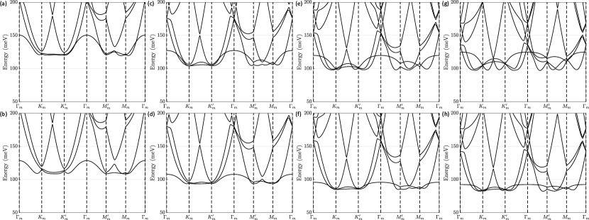
Figure 1: Noninteracting band structure of (a) R3G with $u_{d}=$150\text{\,}\mathrm{m}\mathrm{e}\mathrm{V}$$, (b) R3G with $u_{d}=$128\text{\,}\mathrm{m}\mathrm{e}\mathrm{V}$$, (c) R4G with $u_{d}=$85\text{\,}\mathrm{m}\mathrm{e}\mathrm{V}$$, (d) R4G with $u_{d}=$72\text{\,}\mathrm{m}\mathrm{e}\mathrm{V}$$, (e) R5G with $u_{d}=$60\text{\,}\mathrm{m}\mathrm{e}\mathrm{V}$$, (f) R5G with $u_{d}=$48\text{\,}\mathrm{m}\mathrm{e}\mathrm{V}$$, (g) R6G with $u_{d}=$50\text{\,}\mathrm{m}\mathrm{e}\mathrm{V}$$, and (h) R6G with $u_{d}=$37\text{\,}\mathrm{m}\mathrm{e}\mathrm{V}$$. Here, the twist angle is $\theta=0.77^{\circ}$.

Interacting model of RnG.— In the experiment, the RnG is aligned with one layer of hBN on one side but misaligned on the other side, resulting in a moiré potential on the aligned layer of graphene. The noninteracting continuum model of spin $\sigma$ in such a system can be written as [28, 29, 30],

$$H_{\text{s},\sigma} =H_{\text{RnG}}(-i\nabla)+u_{d}V_{d}+V_{\text{moir\'{e}}}(r),$$ (1)

where the first term is the Hamiltonian of the pristine RnG, the second term is the perpendicular displacement field with $u_{d}$ denoting the voltage between the neighboring layers of the RnG, and the last term is the moiré potential acting only on the aligned layer. Their specific forms will be discussed below. Originating from the lattice mismatch and twist angle between RnG and hBN, the periodicity of the moiré potential determines the moiré Brillouin zone (MBZ) in the momentum space.

We now explain the specific forms of the Hamiltonian $H_{\text{RnG}}$, the displacement field $V_{d}$, and the moiré potential $V_{\text{moir\'{e}}}$ in the RnG. In the momentum space, the Hamiltonian of the pristine RnG is modeled as

$$H_{\text{RnG}}(\mathbf{k})=\left[\begin{array}[]{ccccc}h^{(0)}&h^{(1)}&h^{(2)}&&\\ h^{(1){\dagger}}&h^{(0)}&\ddots&\ddots&\\ h^{(2){\dagger}}&\ddots&\ddots&h^{(1)}&h^{(2)}\\ &\ddots&h^{(1){\dagger}}&h^{(0)}&h^{(1)}\\ &&h^{(2){\dagger}}&h^{(1){\dagger}}&h^{(0)}\end{array}\right],$$ (7)

where

$$h^{(0)}=-t_{0}\left[\begin{array}[]{cc}0&f_{\mathbf{k}}\\ f_{\mathbf{k}}^{*}&0\end{array}\right],\quad h^{(1)}=\left[\begin{array}[]{cc}t_{4}f_{\mathbf{k}}&t_{3}f_{\mathbf{k}}^{*}\\ t_{1}&t_{4}f_{\mathbf{k}}\end{array}\right],$$ (12)

$$h^{(2)}=\left[\begin{array}[]{cc}0&\frac{t_{2}}{2}\\ 0&0\end{array}\right],\quad f_{\mathbf{k}}=\sum_{j}\exp(i\mathbf{k}\cdot\delta_{j}).$$ (15)

Following Ref. [31], we take

$$(t_{0},t_{1},t_{2},t_{3},t_{4})=(3100,380,-21,290,141)\,\text{meV}.$$

Further, the displacement field is given by

$$[V_{d}]_{ll^{\prime}}=\delta_{ll^{\prime}}[l-(n_{l}-1)/2],$$ (16)

where $l,l^{\prime}$ are the indices of layer, and $n_{l}$ is the number of layers. Here, $l=0$ represents the top layer, and $l=n_{l}-1$ represents the bottom layer.

To model the moiré potential, we consider the aligned layer of RnG with hBN. At twist angle $\theta$, the reciprocal basis vectors of the aligned hBN are given by

$$\mathbf{G}_{i}^{\prime}=\frac{a_{\text{G}}}{a_{\text{hBN}}}R_{\theta}\mathbf{G}_{i},\quad(i=1,2),$$ (17)

with a lattice mismatch $a_{\text{hBN}}/a_{\text{G}}\approx 1.018$. Here $\mathbf{G}_{i}$ are the reciprocal lattice vectors of graphene. Hence, the moiré reciprocal vectors are given by the difference between the reciprocal vectors of the RnG and hBN, i.e., $\mathbf{g}_{i}=\mathbf{G}_{i}-\mathbf{G}_{i}^{\prime}$ for $i=1,2$ and $\mathbf{g}_{3}=-\mathbf{g}_{1}-\mathbf{g}_{2}$. In this work, we follow Ref. [30] and take the following form for the moiré potential on the aligned layer in the $\mathbf{K}$ valley,

$$V_{\text{moir\'{e}}}(\mathbf{r})=V_{0}\mathbb{I}+V_{1}\sum_{j=1}^{3}\quantity[e^{i\psi}U_{j}e^{i\mathbf{r}\cdot\mathbf{g}_{j}}+\text{H.c.}],$$ (18)

where

$$U_{1}=\left[\begin{array}[]{cc}1&1\\ \omega&\omega\end{array}\right],\quad U_{2}=\left[\begin{array}[]{cc}1&1/\omega\\ 1/\omega&\omega\end{array}\right],\quad U_{3}=\left[\begin{array}[]{cc}1&\omega\\ 1&\omega\end{array}\right],$$

with $\omega=e^{2\pi/3i}$, $\mathbb{I}$ is identity, and $(V_{0},V_{1},\psi)=(28.9\,\text{meV},21\,\text{meV},0.29)$. The $\mathbf{K}^{\prime}$ valley is defined by the time-reversal symmetry.

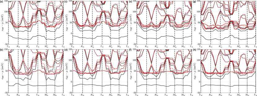
Figure 2: Noninteracting band structure of (a) R3G with $u_{d}=$150\text{\,}\mathrm{m}\mathrm{e}\mathrm{V}$$, (b) R3G with $u_{d}=$128\text{\,}\mathrm{m}\mathrm{e}\mathrm{V}$$, (c) R4G with $u_{d}=$85\text{\,}\mathrm{m}\mathrm{e}\mathrm{V}$$, (d) R4G with $u_{d}=$72\text{\,}\mathrm{m}\mathrm{e}\mathrm{V}$$, (e) R5G with $u_{d}=$60\text{\,}\mathrm{m}\mathrm{e}\mathrm{V}$$, (f) R5G with $u_{d}=$48\text{\,}\mathrm{m}\mathrm{e}\mathrm{V}$$, (g) R6G with $u_{d}=$50\text{\,}\mathrm{m}\mathrm{e}\mathrm{V}$$, and (h) R6G with $u_{d}=$37\text{\,}\mathrm{m}\mathrm{e}\mathrm{V}$$. The black lines denote the spin-up sector, and the red dashed lines denote the spin-down sector. Here, the twist angle is $\theta=0.77^{\circ}$, and the calculation is performed on a $4\times 6$ mesh in the MBZ.

For the many-body interaction, we consider the gated-screened Coulomb interaction, given by

$$V_{\text{Coulomb}}=\frac{1}{2A}\sum_{\mathbf{q}}\dfrac{\tanh(dq)}{2\epsilon\epsilon_{0}q}:\rho_{-\mathbf{q}}\,\rho_{\mathbf{q}}:,$$ (19)

where $A$ is the area of the system, $:\mathcal{O}:$ denotes the normal order of an operator, $d$ is the distance between the sample and the gate (taken to be $100\text{\,}\mathrm{n}\mathrm{m}$), and $\epsilon$ is the background dielectric constant (taken to be $5$ in this work). Here, we define the density operator $\rho_{\mathbf{q}}=\sum_{\alpha,\sigma}\sum_{\mathbf{k}}c_{\mathbf{k}+\mathbf{q},\alpha,\sigma}^{\dagger}c_{\mathbf{k},\alpha,\sigma}$, and $c_{\mathbf{k},\alpha,\sigma}$ denotes the annihilation operator of a plane wave state, where $\alpha$ represents the collective index of layer, sublattice, and valley. The total Hamiltonian is then given by

$$H=\sum_{\sigma}H_{\text{s},\sigma}+V_{\text{Coulomb}}-V_{\text{HF}}(P_{\text{ref}}),$$ (20)

where the third term is induced to avoid double counting the interaction within the momentum cutoff of the continuum model. $V_{\text{HF}}(P)$ denotes the Coulomb interaction in the HF approximation and is a linear functional of the one-body density matrix $P$. $P_{\text{ref}}$ here is the so-called “reference field” or “subtraction scheme”, which does not have an accepted form in the literature. Because of the convergence issue discussed in Ref. [21], we take $P_{\text{ref}}$ to be the noninteracting ground state at the charge neutrality point. This choice of reference field is known in the literature as the charge neutrality scheme, and other possible choices are discussed in Ref. [21].

The IQAH effect in RnG.— The experimental observation of the IQAH and FQAH is theoretically baffling because the noninteracting band structure of the RnG with a strong displacement field is highly entangled and with no discrenible gaps in the spectrum, as shown in Fig. 1. Moreover, we observe that the stronger the displacement field, the more entangled the conduction bands. Hence, a naive noninteracting band structure cannot explain the IQAH effect, let alone the FQAH effect. To resolve this problem, an HF approach is proposed to understand the appearance of the IQAH [16, 17, 18, 19, 20], in which an HF charge gap is formed associated with a spontaneous symmetry breaking leading to a Chern number, separating the lowest HF conduction band from the rest. In Fig. 2, we calculate the HF band structure at filling factor $\nu=1$ in RnG ($n=$36$$) for two values of $u_{d}$. In this work, we always include all the bands within the momentum cutoff in the HF calculation instead of projecting the system to a few valence and conduction bands. For the parameters studied in Fig. 2, we find that the spin-valley polarized solutions are always energetically favored in the HF calculation and that a correlated gap is always formed between the lowest conduction band and the other conduction bands. Furthermore, there is a sweet spot for each of these structures, respectively, where the lowest conduction band becomes considerably flatter, as shown in the bottom row of Fig. 2. Moreover, the HF band is topologically nontrivial with Chern number $C=1$. However, the band width of the lowest quasiparticle conduction band increases significantly as the displacement field deviates from this sweet spot, as shown in the top row of Fig. 2. This clearly establishes the necessity for the applied electric field in obtaining IQAH and FQAH effects in RnG.

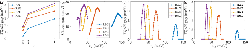
Figure 3: (a) FQAH gap at various filling factors. We take $u_{d}=$128\text{\,}\mathrm{m}\mathrm{e}\mathrm{V}$,$72\text{\,}\mathrm{m}\mathrm{e}\mathrm{V}$,$48\text{\,}\mathrm{m}\mathrm{e}\mathrm{V}$,$37\text{\,}\mathrm{m}\mathrm{e}\mathrm{V}$$ for R3G, R4G, R5G, and R6G, respectively. For $\nu=1$, we show the charge gaps in the HF calculation at $\nu=1$, and we write $\times 5$ for those data points, meaning that the actual gaps are five times as large as the data points in the plot. (b) Charge gap at $\nu=1$, (c) FQAH gap at $\nu=2/3$, and (d) FQAH gap at $\nu=3/5$ as a function of the displacement field. In all panels, the twist angle is $\theta=0.77^{\circ}$, and the calculation is performed on a $4\times 6$ mesh in the MBZ for $\nu=1,2/3$ and on a $5\times 5$ mesh in the MBZ for $\nu=3/5$.

The FQAH effect in RnG.— While the HF calculation can predict the IQAH effect at integer fillings, it fails to capture the strongly correlated ground states at fractional fillings, although it has been hypothesized [24] that a partially filled flat Chern band could result in the FQAH effect. However, this hypothesis must be verified explicitly for each specific case. One of the most reliable methods to investigate the FQAH effect is the exact diagonalization (ED), which is limited to one or two bands. However, there are multiple highly entangled bands in the RnG, far beyond the capability of the ED. Notwithstanding, if one assumes that the electron correlation only appears in the lowest quasiparticle conduction band, the Hamiltonian can be projected to the following subspace [21]

$$\mathcal{P}=\text{span}\quantity\Big{\prod_{i=1}^{N}f_{c,\mathbf{k}_{i}}^{\dagger}\prod_{\alpha,\mathbf{k}}{f_{v,\alpha,\mathbf{k}}^{\dagger}}\ket{0}:\mathbf{k}_{i}\in\text{MBZ}},$$ (21)

where $f_{c,\mathbf{k}}$ is the partially filled quasiparticle conduction band, and $f_{v,\alpha,\mathbf{k}}$ is the completely filled quasiparticle valence bands. In principle, the quasiparticle bands should be determined variationally by minimizing the ground state energy. However, this is numerically impossible. In practice, one can only compare the energies of different candidate sets of quasiparticle bands, and the quasiparticle bands derived from a constrained HF calculation at the corresponding fractional filling are found to produce the most energetically favorable FQAH ground states [21]. Essentially, the constrained HF calculation requires the one-body density matrix to have a uniform density in the MBZ, which is a hallmark of the FQAH states. This method is equivalent to treating the interband interaction on the HF level but treating the intraband interaction within the quasiparticle conduction band on the ED level to generate an FQAH state.

We now study the FQAH state in RnG ($n=$36$$) using a combination of the constrained HF and ED calculations described above. The results are presented in Fig. 3. Here, we characterize the stability of the FQAH phase by the FQAH gap. As the FQAH state follows the generalized Pauli exclusion principle, the degenerate ground states only appear in the dictated momentum sectors [26]. Therefore, the FQAH gap is defined as the energy gap between the highest ground state energy in the dictated momentum sectors and the rest of the energies. In particular, the FQAH gap is set to zero if such a gap does not exist. For the displacement field used in the upper panels of Fig. 1 and Fig. 2, we find that the FQAH gap vanishes in the corresponding system because of the large dispersion in the quasiparticle conduction band. In contrast, for the displacement used in the lower panels of Fig. 1 and Fig. 2, we find a finite FQAH gap at both $\nu=2/3$ and $\nu=3/5$, as shown in Fig. 3(a). We also note that the FQAH gap at $\nu=2/3$ is larger than that at $\nu=3/5$ but much smaller than the charge gap at $\nu=1$.

Finally, we study the energy gaps as a function of the displacement field at different fillings. At filling factor $\nu=1$, the HF calculation always opens up a gap for the parameter range we studied, as shown in Fig. 3(b). However, we indeed observe a competition between HF solutions with different Chern numbers in R5G and R6G, and their transition results in cusps at $u_{d}=$35\text{\,}\mathrm{m}\mathrm{e}\mathrm{V}$$ for R5G and $u_{d}=$28\text{\,}\mathrm{m}\mathrm{e}\mathrm{V}$$ for R6G. At $2/3$ filling, all four systems have a finite region of FQAH states, as shown in Fig. 3(c). We also notice that the necessary displacement field in the R4G to generate FQAH states is stronger than in the R5G. This agrees with the experimental observations, although the experiments of R4G and R5G are performed at two slightly different twist angles [32]. Meanwhile, the displacement field required to generate FQAH states in R3G is significantly larger (this fact may have prevented the experimental manifestation of the FQAH effect in R3G.) We also examine the FQAH effects at $3/5$ filling. The nonvanishing FQAH gap shown in Fig. 3(d) suggests that the FQAH states still exist. However, compared to the $2/3$ filling case, both the range of the FQAH phase and the magnitude of the nonvanishing FQAH gap are smaller, confirming the generic well-known trend that FQHE is less stable for higher-order fractional states.

Discussion and conclusion.— In this work, we have studied the IQAH and FQAH effects in RnG with a strong displacement field. The focus of our study is to apply the comprehensive theory we developed previously for the IQAH and FQAH effects in R5G to other RnG systems and examine the stability of the FQAH phase in these systems. Our results show that under similar conditions, a quasiparticle conduction band with $C=1$ can be formed in RnG at the integer filling $\nu=1$, leading to the IQAH effect. Moreover, upon hole doping the lowest quasiparticle conduction band, the FQAH effect can be observed at certain fractional fillings in RnG in general. Despite this general trend, several interesting features are observed in the FQAH effect in RnG. First, the FQAH gap at $\nu=2/3$ and $\nu=3/5$ generally decreases with the number of layers $n$. Second, the center of the FQAH phase in the displacement field axis is shifted to a larger value as $n$ decreases. This suggests that a very large displacement field may be required to observe the FQAH effect in R3G. However, a quantitative comparison between the FQAH gaps in different RnG systems is currently challenging because of the different parameters used in the experiments, such as the twist angle between the RnG and hBN for different $n$. In addition, current experiments appear to have large background disorder effects [22], making any comparison between theory and experiment impossible since strong disorder would generically suppress both FQAH and IQAH [33].

Acknowledgements.— K.H. and X.L. are supported by the Research Grants Council of Hong Kong (Grants No. CityU 11300421, CityU 11304823, and C7012-21G) and City University of Hong Kong (Projects No. 9610428 and 7005938). K.H. is also supported by the Hong Kong PhD Fellowship Scheme. S.D.S. is supported by the Laboratory for Physical Sciences through the Condensed Matter Theory Center (CMTC) at the University of Maryland. This work was performed in part at the Aspen Center for Physics, which is supported by National Science Foundation grant PHY-2210452.

References

- Chen et al. [2019a] G. Chen, L. Jiang, S. Wu, B. Lyu, H. Li, B. L. Chittari, K. Watanabe, T. Taniguchi, Z. Shi, J. Jung, Y. Zhang, and F. Wang, Evidence of a gate-tunable Mott insulator in a trilayer graphene moiré superlattice, Nat. Phys. 15, 237 (2019a).
- Zhou et al. [2021a] H. Zhou, T. Xie, A. Ghazaryan, T. Holder, J. R. Ehrets, E. M. Spanton, T. Taniguchi, K. Watanabe, E. Berg, M. Serbyn, and A. F. Young, Half- and quarter-metals in rhombohedral trilayer graphene, Nature 598, 429 (2021a).
- Han et al. [2023a] T. Han, Z. Lu, G. Scuri, J. Sung, J. Wang, T. Han, K. Watanabe, T. Taniguchi, H. Park, and L. Ju, Correlated insulator and Chern insulators in pentalayer rhombohedral-stacked graphene, Nat. Nanotechnol. 19, 181 (2023a).
- Winterer et al. [2024] F. Winterer, F. R. Geisenhof, N. Fernandez, A. M. Seiler, F. Zhang, and R. T. Weitz, Ferroelectric and spontaneous quantum Hall states in intrinsic rhombohedral trilayer graphene, Nat. Phys. 20, 422 (2024).
- Arp et al. [2024] T. Arp, O. Sheekey, H. Zhou, C. L. Tschirhart, C. L. Patterson, H. M. Yoo, L. Holleis, E. Redekop, G. Babikyan, T. Xie, J. Xiao, Y. Vituri, T. Holder, T. Taniguchi, K. Watanabe, M. E. Huber, E. Berg, and A. F. Young, Intervalley coherence and intrinsic spin–orbit coupling in rhombohedral trilayer graphene, Nat. Phys. 10.1038/s41567-024-02560-7 (2024).
- Chen et al. [2019b] G. Chen, A. L. Sharpe, P. Gallagher, I. T. Rosen, E. J. Fox, L. Jiang, B. Lyu, H. Li, K. Watanabe, T. Taniguchi, J. Jung, Z. Shi, D. Goldhaber-Gordon, Y. Zhang, and F. Wang, Signatures of tunable superconductivity in a trilayer graphene moiré superlattice, Nature 572, 215 (2019b).
- Zhou et al. [2021b] H. Zhou, T. Xie, T. Taniguchi, K. Watanabe, and A. F. Young, Superconductivity in rhombohedral trilayer graphene, Nature 598, 434 (2021b).
- Han et al. [2023b] T. Han, Z. Lu, G. Scuri, J. Sung, J. Wang, T. Han, K. Watanabe, T. Taniguchi, L. Fu, H. Park, and L. Ju, Orbital multiferroicity in pentalayer rhombohedral graphene, Nature 623, 41 (2023b).
- Liu et al. [2023] K. Liu, J. Zheng, Y. Sha, B. Lyu, F. Li, Y. Park, Y. Ren, K. Watanabe, T. Taniguchi, J. Jia, W. Luo, Z. Shi, J. Jung, and G. Chen, Spontaneous broken-symmetry insulator and metals in tetralayer rhombohedral graphene, Nature Nanotechnology 19, 188 (2023).
- Li et al. [2024] C. Li, F. Xu, B. Li, J. Li, G. Li, K. Watanabe, T. Taniguchi, B. Tong, J. Shen, L. Lu, J. Jia, F. Wu, X. Liu, and T. Li, Tunable superconductivity in electron- and hole-doped Bernal bilayer graphene, Nature 631, 300 (2024).
- Chen et al. [2020] G. Chen, A. L. Sharpe, E. J. Fox, Y.-H. Zhang, S. Wang, L. Jiang, B. Lyu, H. Li, K. Watanabe, T. Taniguchi, Z. Shi, T. Senthil, D. Goldhaber-Gordon, Y. Zhang, and F. Wang, Tunable correlated Chern insulator and ferromagnetism in a moiré superlattice, Nature 579, 56 (2020).
- Han et al. [2024] T. Han, Z. Lu, Y. Yao, J. Yang, J. Seo, C. Yoon, K. Watanabe, T. Taniguchi, L. Fu, F. Zhang, and L. Ju, Large quantum anomalous Hall effect in spin-orbit proximitized rhombohedral graphene, Science 384, 647 (2024).
- Lu et al. [2024] Z. Lu, T. Han, Y. Yao, A. P. Reddy, J. Yang, J. Seo, K. Watanabe, T. Taniguchi, L. Fu, and L. Ju, Fractional quantum anomalous Hall effect in multilayer graphene, Nature 626, 759 (2024).
- Xie et al. [2024] J. Xie, Z. Huo, X. Lu, Z. Feng, Z. Zhang, W. Wang, Q. Yang, K. Watanabe, T. Taniguchi, K. Liu, Z. Song, X. C. Xie, J. Liu, and X. Lu, Even- and Odd-denominator Fractional Quantum Anomalous Hall Effect in Graphene Moire Superlattices (2024), arXiv:2405.16944 [cond-mat.mes-hall] .
- Guo et al. [2023] Z. Guo, X. Lu, B. Xie, and J. Liu, Theory of fractional Chern insulator states in pentalayer graphene moiré superlattice (2023), arXiv:2311.14368 [cond-mat.str-el] .
- Dong et al. [2023a] J. Dong, T. Wang, T. Wang, T. Soejima, M. P. Zaletel, A. Vishwanath, and D. E. Parker, Anomalous Hall Crystals in Rhombohedral Multilayer Graphene I: Interaction-Driven Chern Bands and Fractional Quantum Hall States at Zero Magnetic Field (2023a), arXiv:2311.05568 [cond-mat.str-el] .
- Dong et al. [2023b] Z. Dong, A. S. Patri, and T. Senthil, Theory of fractional quantum anomalous Hall phases in pentalayer rhombohedral graphene moiré structures (2023b), arXiv:2311.03445 [cond-mat.str-el] .
- Zhou et al. [2023] B. Zhou, H. Yang, and Y.-H. Zhang, Fractional quantum anomalous Hall effects in rhombohedral multilayer graphene in the moiréless limit and in Coulomb imprinted superlattice (2023), arXiv:2311.04217 [cond-mat.str-el] .
- Kwan et al. [2023] Y. H. Kwan, J. Yu, J. Herzog-Arbeitman, D. K. Efetov, N. Regnault, and B. A. Bernevig, Moiré Fractional Chern Insulators III: Hartree-Fock Phase Diagram, Magic Angle Regime for Chern Insulator States, the Role of the Moiré Potential and Goldstone Gaps in Rhombohedral Graphene Superlattices (2023), arXiv:2312.11617 [cond-mat.str-el] .
- Yu et al. [2024] J. Yu, J. Herzog-Arbeitman, Y. H. Kwan, N. Regnault, and B. A. Bernevig, Moiré fractional chern insulators iv: Fluctuation-driven collapse of fcis in multi-band exact diagonalization calculations on rhombohedral graphene (2024), arXiv:2407.13770 [cond-mat.str-el] .
- Huang et al. [2024] K. Huang, X. Li, S. Das Sarma, and F. Zhang, Self-consistent theory for the fractional quantum anomalous Hall effect in rhombohedral pentalayer graphene (2024), arXiv:2407.08661 [cond-mat.str-el] .
- Xie and Das Sarma [2024] M. Xie and S. Das Sarma, Integer and fractional quantum anomalous Hall effects in pentalayer graphene, Phys. Rev. B 109, L241115 (2024).
- Tang et al. [2011] E. Tang, J.-W. Mei, and X.-G. Wen, High-Temperature Fractional Quantum Hall States, Phys. Rev. Lett. 106, 236802 (2011).
- Sun et al. [2011] K. Sun, Z. Gu, H. Katsura, and S. Das Sarma, Nearly Flatbands with Nontrivial Topology, Phys. Rev. Lett. 106, 236803 (2011).
- Neupert et al. [2011] T. Neupert, L. Santos, C. Chamon, and C. Mudry, Fractional Quantum Hall States at Zero Magnetic Field, Phys. Rev. Lett. 106, 236804 (2011).
- Regnault and Bernevig [2011] N. Regnault and B. A. Bernevig, Fractional Chern Insulator, Phys. Rev. X 1, 021014 (2011).
- Sheng et al. [2011] D. Sheng, Z.-C. Gu, K. Sun, and L. Sheng, Fractional quantum Hall effect in the absence of Landau levels, Nat. Commun. 2, 389 (2011).
- Zhang et al. [2010] F. Zhang, B. Sahu, H. Min, and A. H. MacDonald, Band structure of -stacked graphene trilayers, Phys. Rev. B 82, 035409 (2010).
- Jung and MacDonald [2013] J. Jung and A. H. MacDonald, Gapped broken symmetry states in ABC-stacked trilayer graphene, Phys. Rev. B 88, 075408 (2013).
- Moon and Koshino [2014] P. Moon and M. Koshino, Electronic properties of graphene/hexagonal-boron-nitride moiré superlattice, Phys. Rev. B 90, 155406 (2014).
- Wang et al. [2024] T. Wang, M. Vila, M. P. Zaletel, and S. Chatterjee, Electrical control of spin and valley in spin-orbit coupled graphene multilayers, Phys. Rev. Lett. 132, 116504 (2024).
- [32] Private communications with Long Ju.
- Yang et al. [2012] S. Yang, K. Sun, and S. Das Sarma, Quantum phases of disordered flatband lattice fractional quantum Hall systems, Phys. Rev. B 85, 205124 (2012).