Cycle-Configuration: A Novel Graph-theoretic Descriptor Set for Molecular Inference

Abstract

In this paper, we propose a novel family of descriptors of chemical graphs, named cycle-configuration (CC), that can be used in the standard “two-layered (2L) model” of mol-infer, a molecular inference framework based on mixed integer linear programming (MILP) and machine learning (ML). Proposed descriptors capture the notion of ortho/meta/para patterns that appear in aromatic rings, which has been impossible in the framework so far. Computational experiments show that, when the new descriptors are supplied, we can construct prediction functions of similar or better performance for all of the 27 tested chemical properties. We also provide an MILP formulation that asks for a chemical graph with desired properties under the 2L model with CC descriptors (2L$+$CC model). We show that a chemical graph with up to 50 non-hydrogen vertices can be inferred in a practical time.

1 Introduction

Among key issues in cheminformatics and bioinformatics is the problem of inferring molecules that are expected to attain desired activities/properties. This problem is also known as inverse QSAR/QSPR modeling [13, 23]. We focus our attention on inverse QSAR/QSPR modeling of low molecular weight organic compounds, which has applications in drug discovery [17, 28] and material science [19]. With recent rapid progress of machine learning (ML), there have been developed a lot of inverse QSAR/QSPR models, most of which are based on neural networks (NNs); e.g., variational autoencoders [8], generative adversarial networks [7, 21], and invertible flow models [16, 24]. The weakness of NN based methods is the lack of optimality and exactness [30], where we mean by optimality the preciseness of a solution to attain the desired activities/properties; and by exactness the guarantee of a solution as a valid molecule. Besides, it is hard to exploit domain knowledge in NN based methods.

Our research group has developed a new framework of molecular inference that is based on mixed integer linear programming (MILP) and ML. This framework, which we call mol-infer, achieves optimality and exactness, and enables practitioners to exploit domain knowledge to some extent. Let ${\mathcal{G}}$ denote the set of all possible chemical graphs. The process of mol-infer is summarized as follows.

Stage 1:

Determine the target chemical property $\pi$ and collect a data set $D_{\pi}\subseteq{\mathcal{G}}$ of chemical graphs such that the observed value $a({\mathbb{C}})$ for the chemical property $\pi$ is available for all chemical graphs ${\mathbb{C}}\in D_{\pi}$.

Stage 2:

Design a set of descriptors to obtain a feature function $f:{\mathcal{G}}\to{\mathbb{R}}^{K}$ that converts a chemical graph ${\mathbb{C}}\in D_{\pi}$ into a $K$-dimensional real feature vector $f({\mathbb{C}})\in{\mathbb{R}}^{K}$, where $K$ is the number of descriptors.

Stage 3:

Construct a prediction function $\eta:{\mathbb{R}}^{K}\to{\mathbb{R}}$ from the data set $f(D_{\pi})\triangleq\{f({\mathbb{C}})\mid{\mathbb{C}}\in D_{\pi}\}$ of feature vectors, where $\eta({\mathbb{C}})$ is used to estimate the property value $a({\mathbb{C}})$ of a chemical graph ${\mathbb{C}}$.

Stage 4:

Determine two real numbers $\underline{y}^{\ast},\overline{y}^{\ast}$ $(\underline{y}^{\ast}\leq\overline{y}^{\ast})$ as lower/upper bounds on the target value and a set $\sigma$ of rules (called a specification) on chemical graphs. Let ${\mathcal{G}}_{\sigma}\subseteq{\mathcal{G}}$ denote the set of all chemical graphs that satisfy $\sigma$. Formulate the problem of constructing a chemical graph ${\mathbb{C}}^{\dagger}$ as MILP whose constraints include ${\mathcal{C}}_{1}$ and ${\mathcal{C}}_{2}$ to ensure $({\mathcal{C}}_{1})$ $\underline{y}^{\ast}\leq\eta(f({\mathbb{C}}^{\dagger}))\leq\overline{y}^{\ast}$ and $({\mathcal{C}}_{2})$ ${\mathbb{C}}^{\dagger}\in{\mathcal{G}}_{\sigma}$. Solve the MILP to obtain ${\mathbb{C}}^{\dagger}$. If the MILP is infeasible, then it is indicated that no such ${\mathbb{C}}^{\dagger}$ exist.

Stage 5:

Generate isomers of ${\mathbb{C}}^{\dagger}$ somehow.

Regarded as a method of inverse QSAR/QSPR, the highlight of mol-infer is Stage 4 that solves the inverse problem by MILP, which is the original contribution of this framework. For ${\mathcal{C}}_{1}$, the process of computing the feature vector $f({\mathbb{C}})$ for a chemical graph ${\mathbb{C}}$ and the process of computing the prediction value $\eta(x)$ of a feature vector $x=f({\mathbb{C}})$ must be represented by linear inequalities of real and/or integer variables. It is shown that artificial neural network [1], linear regression [31] and decision tree [26] can be used as $\eta$. We will discuss how to design $f$ for this purpose in the next paragraph. For ${\mathcal{C}}_{2}$, in our early studies, we could deal with only limited classes of chemical graphs; e.g., trees [4, 29], rank-1 graphs [14] and rank-2 graphs [33]. Shi et al.’s two-layered (2L) model [25] admits us to infer any chemical graph, where users are required to design an abstract structure of ${\mathbb{C}}^{\dagger}$ as a part of the specification $\sigma$. Stage 5 is not within the scope of this paper. For this stage, a dynamic programming algorithm [32] and a grid neighborhood approach [3] are developed. Furthermore, mol-infer is applied to the inference of polymers [12].

Let us describe how we design the feature function $f$ in Stage 2. The descriptors should be informative since they have a great influence on prediction performance in Stage 3 and thus on the quality of chemical graphs that we finally obtain as a result of Stages 4 and 5; if the prediction function $\eta$ is not accurate enough, then we could not expect the inferred graphs to have desired property. On the other hand, as mentioned above, the process of computing descriptor values should be represented by a set of linear inequalities. It is hard to include descriptors of complicated concepts. There is a trade-off between informativity and simplicity in the design of descriptors.

Due to these reasons, mol-infer employs graph-theoretic descriptors that capture local information of chemical graphs and that are somewhat similar to typical fingerprints. Let $f_{\textrm{2L}}$ be a feature function in the 2L model, the standard model in mol-infer. The 2L model has a weak point such that there are distinct chemical graphs ${\mathbb{C}}_{1},{\mathbb{C}}_{2}$ for which $f_{\textrm{2L}}({\mathbb{C}}_{1})=f_{\textrm{2L}}({\mathbb{C}}_{2})$ holds although $a({\mathbb{C}}_{1})$ and $a({\mathbb{C}}_{2})$ are much different. An example of such ${\mathbb{C}}_{1}$ and ${\mathbb{C}}_{2}$ is shown in Figure 1, where the details are explained in Section 3.1. This issue comes from that the descriptors of the 2L model cannot capture how edges are connected to cycles. For example, although the descriptors can distinguish ortho patterns of an aromatic ring (e.g., ${\mathbb{C}}_{0}$ in Figure 1) from meta/para patterns (e.g., ${\mathbb{C}}_{1}$ and ${\mathbb{C}}_{2}$ in Figure 1, respectively), they fail to distinguish meta and para patterns.

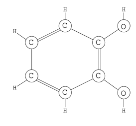
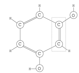
(a)	(b)
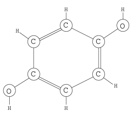
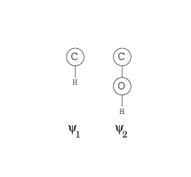
(c)	(d)

Figure 1: (a) the chemical graph ${\mathbb{C}}_{0}$ for catechol; (b) the chemical graph ${\mathbb{C}}_{1}$ for resorcinol; (c) the chemical graph ${\mathbb{C}}_{2}$ for hydroquinone; and (d) two fringe-trees $\psi_{1}$ and $\psi_{2}$ that appearing in all of ${\mathbb{C}}_{0}$, ${\mathbb{C}}_{1}$ and ${\mathbb{C}}_{2}$. In (b), the edge-configuration of the interior-edge indicated by a dotted rectangle is $({\mathtt{C}}2,{\mathtt{C}}3,2)$. Although $f_{\textrm{2L}}({\mathbb{C}}_{1})=f_{\textrm{2L}}({\mathbb{C}}_{2})$, $a({\mathbb{C}}_{1})=0\neq 1=a({\mathbb{C}}_{2})$ holds in the data set of AhR property from Tox21 collection.

In this paper, aiming at overcoming the above weak point in the 2L model, we propose a novel set of descriptors, named cycle-configurations (CC). CC can specify how exterior parts (called “fringe-trees”) are attached to a cycle, by which meta/para patterns in an aromatic ring are distinguishable. Let us denote by $f_{\textrm{CC}}$ a feature function that consists of CC descriptors.

We call the 2L model with CC descriptors the 2L$+$CC model. In the 2L$+$CC model, we use the feature function $f:{\mathcal{G}}\to{\mathbb{R}}^{K}$ such that $f({\mathbb{C}}):=(f_{\textrm{2L}}({\mathbb{C}}),f_{\textrm{CC}}({\mathbb{C}}))$ for a chemical graph ${\mathbb{C}}$ (i.e., concatenation of two feature vectors $f_{\textrm{2L}}({\mathbb{C}})$ and $f_{\textrm{CC}}({\mathbb{C}})$).

Computational experiments show that, by using the 2L$+$CC model, we can construct prediction functions of similar or better performance for all of the 27 tested chemical properties, in comparison with the 2L model. We also provide an MILP formulation for the 2L$+$CC model that asks for a chemical graph with desired properties. We show that a chemical graph with up to 50 non-hydrogen vertices can be inferred in a couple of minutes.

The paper is organized as follows. We make preparations and review the 2L model in Section 2. In Section 3, we describe further background of CC and provide its formal definition. In Section 4, we describe the idea of the MILP for the 2L+CC model. We present computational results in Section 5 and conclude the paper in Section 6. Some details are explained in Appendix.

2 Preliminaries

2.1 Notations and Terminologies

Let ${\mathbb{R}}$, ${\mathbb{R}}_{+}$, ${\mathbb{Z}}$ and ${\mathbb{Z}}_{+}$ denote the sets of reals, non-negative reals, integers, and non-negative integers, respectively. For $p,q\in{\mathbb{Z}}$, let us denote $[p,q]:=\{p,p+1,\dots,q\}$. For a vector (or a sequence) $x\in{\mathbb{R}}^{p}$ and $j\in[1,p]$, we denote by $x(j)$ the $j$-th entry of $x$. We denote $|x|:=p$.

Let $A$ be a finite set. To encode elements in $A$ by integers, we may assume a bijection $\sigma:A\to[1,|A|]$ implicitly. For $a\in A$, we represent the coded integer $\sigma(a)$ by $[a]_{A}$ or simply $[a]$ if $A$ is clear from the context.

For an undirected graph $G$, we denote by $V(G)$ and $E(G)$ the sets of vertices and edges, respectively. For $V^{\prime}\subseteq V(G)$ (resp., $E^{\prime}\subseteq E(G)$), we denote by $G-V^{\prime}$ (resp., $G-E^{\prime}$) the subgraph of $G$ that is obtained by removing the vertices in $V^{\prime}$ along with the incident edges (resp., removing the edges in $E^{\prime}$). When $V^{\prime}=\{v\}$ (resp., $E^{\prime}=\{e\}$), we write $G-\{v\}$ as $G-v$ (resp., $G-\{e\}$ as $G-e$).

A cycle $C$ in a graph $G$ is a subgraph of $G$ such that $V(C)=\{u_{1},u_{2},\dots,u_{\ell}\}$ and $E(C)=\{u_{1}u_{2},\dots,u_{\ell-1}u_{\ell},u_{\ell}u_{1}\}$. We call $C$ chordless if there is no edge in $E(G)\setminus E(C)$ that joins vertices in $V(C)$. The length of a cycle $C$ is denoted by $\mathrm{len}(C)$ (i.e., $\mathrm{len}(C)=|V(C)|=|E(C)|=\ell$). When the length is $\ell$, we call $C$ an $\ell$-cycle.

A graph is rooted if it has a designated vertex, called a root. For a graph $G$ possibly with a root, a leaf-vertex is a non-root vertex with degree 1. We call the edge that is incident to a leaf-vertex a leaf-edge. We denote by $V_{\textrm{leaf}}(G)$ and $E_{\textrm{leaf}}(G)$ the sets of leaf-vertices and leaf-edges in $G$, respectively. For $i\in{\mathbb{Z}}_{+}$, we define the graph $G_{i}$ to be the subgraph of $G$ that is obtained by deleting the set of leaf-vertices $i$ times, that is, $G_{0}:=G$; and $G_{i+1}:=G_{i}-V_{\textrm{leaf}}(G_{i})$. We define the height $0pt(v)$ of a vertex $v\in V_{\textrm{leaf}}(G_{i})$ to be $i$. Note that the height is not defined for all vertices.

2.2 Modeling of Chemical Compounds

We employ the modeling of chemical compounds that was introduced by Zhu et al. [31].

Let us represent chemical elements by H (hydrogen), C (carbon), O (oxygen), N (nitrogen) and so on. To distinguish a chemical element a with multiple valences such as S (sulfur), we denote a with a valence $i$ by a_(i), where we omit the suffix $(i)$ for a chemical element with a unique valence. Let $\Lambda$ be a set of chemical elements; e.g., $\Lambda=\{{\mathtt{H}},{\mathtt{C}},{\mathtt{O}},{\mathtt{N}},{\mathtt{P}},{\mathtt{S}}_{(2)},{\mathtt{S}}_{(4)},{\mathtt{S}}_{(6)}\}$. We represent the valence of ${\mathtt{a}}\in\Lambda$ by a function $\mathrm{val}:\Lambda\to[1,6]$; e.g., $\mathrm{val}({\mathtt{H}})=1$, $\mathrm{val}({\mathtt{C}})=4$, $\mathrm{val}({\mathtt{O}})=2$, $\mathrm{val}({\mathtt{P}})=5$, $\mathrm{val}({\mathtt{S}}_{(2)})=2$ and $\mathrm{val}({\mathtt{S}}_{(6)})=6$. We denote the mass of ${\mathtt{a}}\in\Lambda$ by $\mathrm{mass}^{*}({\mathtt{a}})$.

We represent a chemical compound by a chemical graph that is defined to be ${\mathbb{C}}=(H,\alpha,\beta)$ consisting of a simple, connected undirected graph $H$ and functions $\alpha:V(H)\to\Lambda$ and $\beta:E(H)\to[1,3]$. The set of atoms and the set of bonds in the compound correspond to the vertex set $V(H)$ and the edge set $E(H)$, respectively. The chemical element assigned to $v\in V(H)$ is represented by $\alpha(v)$ and the bond-multiplicity between two adjacent vertices $u,v\in V(H)$ is represented by $\beta(e)$ of the edge $e=uv\in E(H)$. We denote the mass of $H$ by $\mathrm{mass}^{*}(H):=\sum_{v\in V(H)}\mathrm{mass}^{*}(\alpha(v))$.

Let ${\mathbb{C}}=(H,\alpha,\beta)$ be a chemical graph. For a vertex $u\in V(H)$, we denote by $\beta_{\mathbb{C}}(u)$ the sum of bond-multiplicities of edges incident to $u$; i.e., $\displaystyle\beta_{\mathbb{C}}(u):=\sum_{uv\in E(H)}\beta(uv)$. We denote by $\deg_{\mathbb{C}}(u)$ the number of vertices adjacent to $u$ in ${\mathbb{C}}$. For ${\mathtt{a}}\in\Lambda$, we denote by $V_{{\mathtt{a}}}({\mathbb{C}})$ the set of vertices in $v\in V(H)$ such that $\alpha(v)={\mathtt{a}}$ in ${\mathbb{C}}$. We define the hydrogen-suppressed chemical graph of ${\mathbb{C}}$, denoted by $\langle{\mathbb{C}}\rangle$, to be the graph that is obtained by removing all vertices in $V_{{\mathtt{H}}}({\mathbb{C}})$ from $H$.

Two chemical graphs ${\mathbb{C}}_{i}=(H_{i},\alpha_{i},\beta_{i})$, $i=1,2$ are called isomorphic if they admit an isomorphism, i.e., a bijection $\phi:V(H_{1})\to V(H_{2})$ such that “$uv\in E(H_{1})$, $\alpha_{1}(u)={\mathtt{a}}$, $\alpha_{1}(v)={\mathtt{b}}$, $\beta_{1}(uv)=m$” $\Leftrightarrow$ “$\phi(u)\phi(v)\in E(H_{2})$, $\alpha_{2}(\phi(u))={\mathtt{a}}$, $\alpha_{2}(\phi(v))={\mathtt{b}}$, $\beta_{2}(\phi(u)\phi(v))=m$”. Furthermore, when $H_{i}$ is a rooted graph such that $r_{i}\in V(H_{i})$ is the root, $i=1,2$, ${\mathbb{C}}_{1}$ and ${\mathbb{C}}_{2}$ are called rooted-isomorphic if they admit an isomorphism such that $\phi(r_{1})=(r_{2})$.

2.3 Two-Layered (2L) Model

We review the 2L model that was introduced by Shi et al. [25].

2.3.1 Interior and Exterior

Let ${\mathbb{C}}=(H,\alpha,\beta)$ be a chemical graph and $\rho\geq 1$ be an integer, which we call a branch-parameter, where we use $\rho=2$ as the standard value. In the 2L model, the hydrogen-suppressed chemical graph $\langle{\mathbb{C}}\rangle$ is partitioned into “interior” and “exterior” parts as follows. We call a vertex $v\in V(\langle{\mathbb{C}}\rangle)$ an exterior-vertex if $0pt(v)<\rho$, and an edge $e\in E(\langle{\mathbb{C}}\rangle)$ an exterior-edge if $e$ is incident to an exterior-vertex. Let $V^{\textrm{ex}}({\mathbb{C}})$ and $E^{\textrm{ex}}({\mathbb{C}})$ denote the sets of exterior-vertices and exterior-edges, respectively. Define $V^{\textrm{int}}({\mathbb{C}}):=V(\langle{\mathbb{C}}\rangle)\setminus V^{\textrm{ex}}({\mathbb{C}})$ and $E^{\textrm{int}}({\mathbb{C}}):=E(\langle{\mathbb{C}}\rangle)\setminus E^{\textrm{ex}}({\mathbb{C}})$. We call a vertex in $V^{\textrm{int}}({\mathbb{C}})$ an interior-vertex and an edge in $E^{\textrm{int}}({\mathbb{C}})$ an interior-edge. We define the interior ${\mathbb{C}}^{\textrm{int}}$ of ${\mathbb{C}}$ to be the subgraph $(V^{\textrm{int}}({\mathbb{C}}),E^{\textrm{int}}({\mathbb{C}}))$.

The set $E^{\textrm{ex}}({\mathbb{C}})$ of exterior-edges forms a collection of connected graphs such that each is a tree $T$ rooted at an interior vertex $v\in V(T)$ Let ${\mathcal{T}}^{\textrm{ex}}(\langle{\mathbb{C}}\rangle)$ denote the family of such chemical rooted trees in $\langle{\mathbb{C}}\rangle$. For each interior-vertex $u\in V^{\textrm{int}}({\mathbb{C}})$, let $T_{u}\in{\mathcal{T}}^{\textrm{ex}}(\langle{\mathbb{C}}\rangle)$ denote the chemical tree rooted at $u$, where $T_{u}$ may consist only of the vertex $u$. We define the fringe-tree of $u$, denoted by ${\mathbb{C}}[u]$, to be the chemical rooted tree that is obtained by putting back hydrogens to $T_{u}$ that are originally attached in ${\mathbb{C}}$.

2.3.2 Feature Function

For a feature function $f_{\textrm{2L}}$ in the 2L model (Stage 2), there are two types of descriptors: static ones and enumerative ones. There are 14 static descriptors such as the number of non-hydrogen atoms and the number of interior vertices. The enumerative descriptors mainly consist of the frequency of local patterns that appear in a chemical graph ${\mathbb{C}}=(H,\alpha,\beta)$. Examples of such local patterns include “fringe-configurations”, “adjacency-configurations” and “edge-configurations”. We collect enumerative descriptors from a given data set $D_{\pi}$.

Let $u\in V^{\textrm{int}}({\mathbb{C}})$ be an interior-vertex. The fringe-configuration of $u$ is the chemical tree ${\mathbb{C}}[u]$ that is rooted at $u$. Let us denote by ${\mathcal{F}}(D_{\pi})$ the set of all fringe trees that appear in the data set $D_{\pi}$. For each $\psi\in{\mathcal{F}}(D_{\pi})$, we introduce a descriptor that evaluates the number of interior-vertices $u\in V^{\textrm{int}}({\mathbb{C}})$ such that ${\mathbb{C}}[u]$ is rooted-isomorphic to $\psi$.

For an interior-edge $e=uv\in E^{\textrm{int}}({\mathbb{C}})$, let $\alpha(u)={\mathtt{a}}$, $\deg_{\langle{\mathbb{C}}\rangle}(u)=d$, $\alpha(v)={\mathtt{b}}$, $\deg_{\langle{\mathbb{C}}\rangle}(v)=d^{\prime}$ and $\beta(e)=m$. The adjacency-configuration of $e$ (resp., edge-configuration of $e$) is defined to be the tuple $({\mathtt{a}},{\mathtt{b}},m)$ (resp., $({\mathtt{a}}d,{\mathtt{b}}d^{\prime},m)$). Let us denote by $\Gamma_{\textrm{ac}}(D_{\pi})$ (resp., $\Gamma_{\textrm{ec}}(D_{\pi})$) the set of all adjacency-configurations (resp., edge-configurations) in the data set $D_{\pi}$. For each tuple $\gamma_{\textrm{ac}}\in\Gamma_{\textrm{ac}}(D_{\pi})$ (resp., $\gamma_{\textrm{ec}}\in\Gamma_{\textrm{ec}}(D_{\pi})$), we introduce a descriptor that evaluates the number of interior-edges $e\in E^{\textrm{int}}({\mathbb{C}})$ such that the adjacency-configuration (resp., edge-configuration) is equal to $\gamma_{\textrm{ac}}$ (resp., $\gamma_{\textrm{ec}}$).

See Appendix A for a full description of descriptors in the 2L model.

2.3.3 Specification for MILP

In the 2L model, the specification $\sigma$ for MILP (Stage 4) consists of the following three rules:

• a seed graph $G_{\textrm{C}}$ as an abstract form of a target chemical graph ${\mathbb{C}}^{\dagger}$;

• a set ${\mathcal{F}}$ of fringe trees as candidates for a tree ${\mathbb{C}}^{\dagger}[u]$ rooted at each interior-vertex in ${\mathbb{C}}^{\dagger}$; and

• lower/upper bounds on the number of various parameters in ${\mathbb{C}}^{\dagger}$; e.g., chemical elements, double/triple bonds, and fringe/edge/adjacency-configurations.

The MILP formulates the process of constructing a chemical graph ${\mathbb{C}}^{\dagger}$ as follows. First, we decide the interior of ${\mathbb{C}}^{\dagger}$ by “expanding” the seed graph $G_{\textrm{C}}$; e.g., subdividing an edge and attaching a new path to a vertex. Second, regarding all vertices in the expanded seed graph as the interior-vertices of ${\mathbb{C}}^{\dagger}$, we assign a fringe tree in ${\mathcal{F}}$ to every vertex to make the exterior of ${\mathbb{C}}^{\dagger}$. Finally, we assign bond-multiplicities to the interior-edges so that all constraints in $\sigma$ are satisfied. We can regard ${\mathcal{G}}_{\sigma}$ in Section 1 as the set of all chemical graphs that can be constructed in this way. See the preprint of [31] for details of MILP in the 2L model.

3 Cycle-Configurations

In this section, we propose a new type of descriptors for the 2L model, named cycle-configurations (CC).

3.1 Motivation

Let us point out a weak point of the 2L model again; there are chemical graphs that are not isomorphic to each other but are converted into an identical feature vector. See Figure 1 for an example. Three chemical graphs ${\mathbb{C}}_{0}$ (catechol), ${\mathbb{C}}_{1}$ (resorcinol) and ${\mathbb{C}}_{2}$ (hydroquinone) are shown, where ${\mathbb{C}}_{0}$ is the ortho-isomer, ${\mathbb{C}}_{1}$ is the meta-isomer and ${\mathbb{C}}_{2}$ is the para-isomer.

We can confirm that $f_{\textrm{2L}}({\mathbb{C}}_{1})=f_{\textrm{2L}}({\mathbb{C}}_{2})$ holds by observing the descriptors one by one. For fringe-configuration, both chemical graphs contain four $\psi_{1}$ and two $\psi_{2}$ as fringe-trees in common. For edge-configuration, they contain one $({\mathtt{C}}2,{\mathtt{C}}2,1)$; one $({\mathtt{C}}2,{\mathtt{C}}2,2)$; two $({\mathtt{C}}2,{\mathtt{C}}3,1)$ and two $({\mathtt{C}}2,{\mathtt{C}}3,2)$ in common. In this way, one sees that the two chemical graphs take the same values for the other descriptors (see Appendix A). We also see that $f_{\textrm{2L}}({\mathbb{C}}_{0})\neq f_{\textrm{2L}}({\mathbb{C}}_{1})$ and $f_{\textrm{2L}}({\mathbb{C}}_{0})\neq f_{\textrm{2L}}({\mathbb{C}}_{2})$ hold since ${\mathbb{C}}_{0}$ contains one $({\mathtt{C}}2,{\mathtt{C}}2,1)$; two $({\mathtt{C}}2,{\mathtt{C}}2,2)$; two $({\mathtt{C}}2,{\mathtt{C}}3,1)$ and one $({\mathtt{C}}3,{\mathtt{C}}3,2)$ for its edge-configurations, which are different from those of ${\mathbb{C}}_{1}$ and ${\mathbb{C}}_{2}$.

Although the two chemical graphs ${\mathbb{C}}_{1}$ and ${\mathbb{C}}_{2}$ are converted into an identical feature vector, they may have different properties from each other. For example, Tox21 is a collection of data sets for binary classification (i.e., $a({\mathbb{C}})\in\{0,1\}$ for ${\mathbb{C}}\in D_{\pi}$). In AhR data set, the two chemical graphs ${\mathbb{C}}_{1}$ and ${\mathbb{C}}_{2}$ in Figure 1 satisfy $f_{\textrm{2L}}({\mathbb{C}}_{1})=f_{\textrm{2L}}({\mathbb{C}}_{2})$ although $a({\mathbb{C}}_{1})=0$ and $a({\mathbb{C}}_{2})=1$ hold. It is desirable to convert as many such pairs into distinct feature vectors as possible.

3.2 Definitions

We define a new descriptor, cycle-configuration, in order to convert chemical graphs like ${\mathbb{C}}_{1}$ and ${\mathbb{C}}_{2}$ in Figure 1 into distinct feature vectors. Let $R=\{a_{1},a_{2},\dots,a_{k}\}$ be a set of distinct real numbers. For $a\in R$, we define $\mathrm{rank}_{R}(a):=i$ if $a$ is the $i$-th smallest in $R$. For example, when $R=\{3,2,5,9\}$, we have $\mathrm{rank}_{R}(3)=2$, $\mathrm{rank}_{R}(2)=1$, $\mathrm{rank}_{R}(5)=3$, and $\mathrm{rank}_{R}(9)=4$.

Suppose that a chemical graph ${\mathbb{C}}$ is given. Let $C$ be a chordless cycle in ${\mathbb{C}}$ such that $V(C)=\{u_{1},u_{2},\dots,u_{\ell}\}$ and $E(C)=\{u_{1}u_{2},u_{2}u_{3},\dots,u_{\ell-1}u_{\ell},u_{\ell}u_{1}\}$. For $u_{i}\in V(C)$, we define $\mu_{i}:=\mathrm{mass}^{\ast}({\mathbb{C}}[u_{i}])$. Let $R$ denote the set of distinct numbers in $\mu_{1},\mu_{2},\dots,\mu_{\ell}$. We define $\xi(C)$ to be the smallest sequence $(\mathrm{rank}_{R}(\mu_{1}),\mathrm{rank}_{R}(\mu_{2}),\dots,\mathrm{rank}_{R}(\mu_{\ell}))$ with respect to the lexicographic order among all possible cyclic permutations (including reversal) of $(u_{1},u_{2},\dots,u_{\ell})$, where there are $2\ell$ permutations possible. We define the cycle-configuration of $C$ to be $\xi(C)$.

Let us see Figure 1 for example. Suppose $\mathrm{mass}^{\ast}({\mathtt{H}})=1$, $\mathrm{mass}^{\ast}({\mathtt{C}})=12$ and $\mathrm{mass}^{\ast}({\mathtt{O}})=16$. For the two fringe-trees $\psi_{1}$ and $\psi_{2}$ in the figure, we have $\mathrm{mass}^{\ast}(\psi_{1})=12+1=13$ and $\mathrm{mass}^{\ast}(\psi_{2})=12+16+1=29$. Let us denote the unique (chordless) 6-cycle in ${\mathbb{C}}_{i}$ by $C_{i}$, $i=1,2$. The set of distinct numbers that appear as the mass of a fringe-tree is $R=\{13,29\}$ for both chordless cycles, where $\mathrm{rank}_{R}(13)=1$ and $\mathrm{rank}_{R}(29)=2$. One readily sees that $\xi(C_{1})=\xi_{1}:=(1,1,1,2,1,2)$ and $\xi(C_{2})=\xi_{2}:=(1,1,2,1,1,2)$.

CCs are enumerative descriptors, and we collect ones that are included in the feature function from a given data set $D_{\pi}$. We denote by $\Xi(D_{\pi})$ the set of all cycle-configurations $\xi$ that appear in $D_{\pi}$. Let $K_{\textrm{CC}}:=|\Xi(D_{\pi})|$. For a chemical graph ${\mathbb{C}}\in D_{\pi}$, we define $f_{\textrm{CC}}({\mathbb{C}})$ to be a $K_{\textrm{CC}}$-dimensional feature vector $f_{\textrm{CC}}({\mathbb{C}})=(\mathrm{dcp}^{\circ}_{1}({\mathbb{C}}),\mathrm{dcp}^{\circ}_{2}({\mathbb{C}}),\dots,\mathrm{dcp}^{\circ}_{K_{\textrm{CC}}}({\mathbb{C}}))$, where

$\mathrm{dcp}^{\circ}_{i}({\mathbb{C}})$, $i=[\xi^{\ast}]$, $\xi^{\ast}\in\Xi(D_{\pi})$: the number of chordless cycles $C$ in ${\mathbb{C}}$ such that $\xi(C)=\xi^{\ast}$.

See Figure 1 again. Suppose $\Xi(D_{\pi})=\{\xi_{1},\xi_{2},\xi_{3},\xi_{4}\}$ for $\xi_{3}:=(1,1,2,3)$ and $\xi_{4}:=(1,1,1,1,2)$. Then $f_{\textrm{CC}}({\mathbb{C}}_{1})=(1,0,0,0)$ and $f_{\textrm{CC}}({\mathbb{C}}_{2})=(0,1,0,0)$ hold, by which we have $f({\mathbb{C}}_{1})=(f_{\textrm{2L}}({\mathbb{C}}_{1}),f_{\textrm{CC}}({\mathbb{C}}_{1}))\neq(f_{\textrm{2L}}({\mathbb{C}}_{2}),f_{\textrm{CC}}({\mathbb{C}}_{2}))=f({\mathbb{C}}_{2})$.

In our implementation, as $D_{\pi}$ may contain too many CC descriptors, we use only CC descriptors whose lengths are in the range $[c_{\min},c_{\max}]$, where $c_{\min}$ and $c_{\max}$ are positive constants $(c_{\min}\leq c_{\max})$. We will set $c_{\min}:=4$ and $c_{\max}:=6$ since, in most of chemical compounds in conventional databases, the chemical graph is acyclic or contain only chordless cycles whose lengths are within $[4,6]$. See Table 1. For example, in PubChem, among 92,509,596 molecules that are feasible in the 2L-model, 83,520,760 molecules (90%) satisfy this condition.

Table 1: The numbers of chemical compounds in conventional databases. The 2nd to 5th columns represent the number of all registered chemical compounds; the number of feasible chemical graphs in the 2L-model (e.g., connected, at least four carbon atoms exist); the number of chemical graphs that are either acyclic or $\ell(C)\in[4,6]$ for all chordless cycles $C$; the number of chemical graphs that contain none of (i) or (ii), respectively. The percentages indicate the ratio of the number over the left number.

Database	All	2L-model	Acyclic or $\ell(C)\in[4,6]$	No substructures
		feasible	for all chordless cycles $C$	(i) or (ii) in Section 4
PubChem	97,092,888	92,509,596	83,520,760	80,842,345
(as of 2019)		(95%)	(90%)	(96%)
QM9	130,786	130,786	71,520	60,352
		(100%)	(54%)	(84%)
Tox21	8,014	7,769	7,273	7,080
		(96%)	(93%)	(97%)

4 MILP Formulation for 2L$+$CC Model

Let us consider an MILP formulation for inferring a chemical graph in the 2L$+$CC model. Similarly to the 2L model, the constraints of the MILP consist of $({\mathcal{C}}_{1})$ $\underline{y}^{\ast}\leq\eta(f({\mathbb{C}}^{\dagger}))\leq\overline{y}^{\ast}$ and $({\mathcal{C}}_{2})$ ${\mathbb{C}}^{\dagger}\in{\mathcal{G}}_{\sigma}$, where ${\mathbb{C}}^{\dagger}$ denotes a chemical graph to be inferred and is represented by real/integer variables. We can use any prediction function $\eta$ in ${\mathcal{C}}_{1}$ if its computational process can be represented by a set of linear inequalities. For example, artificial neural network [1], linear regression [31] and decision tree [26] can be used to construct $\eta$. In this section, we overview how we formulate ${\mathcal{C}}_{2}$ as MILP. See Appendix B for the precise formulation of the MILP that includes how we represent the computational process of the feature function $f$ by a set of linear inequalities.

The basic idea of ${\mathcal{C}}_{2}$ is similar to the 2L model (see Section 2.3.3); we represent by ${\mathcal{C}}_{2}$ the computational process of expanding an abstract form of the chemical graph to a concrete chemical graph. We introduce a new type of abstract form, which we call a “seed tree”, since it is hard to deal with CC descriptors by a seed graph of the 2L model.

A seed tree is a tuple ${\mathcal{T}}=(T;V^{\circ},E^{\circ})$ of an unrooted tree $T$, $V^{\circ}\subseteq V(T)$ and $E^{\circ}\subseteq\{uv\in E(T)\mid u,v\in V^{\circ}\}$. We call a node in $V^{\circ}$ a ring node and an edge in $E^{\circ}$ a ring edge, whereas a node in $V(T)\setminus V^{\circ}$ is a non-ring node, and an edge in $E(T)\setminus E^{\circ}$ is a non-ring edge. For a node $u\in V(T)$, we denote by $E^{\circ}(u)$ and $\bar{E}^{\circ}(u)$ the sets of all ring edges and of all non-ring edges incident to $u$, respectively. See Figure 2(a) for an example.

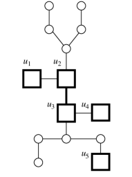
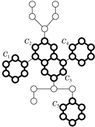
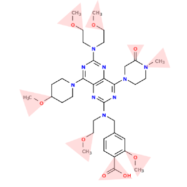
(a)	(b)	(c)

Figure 2: Construction of a chemical graph. (a) A seed tree. Thick squares/lines indicate ring nodes/edges, while thin circles/lines indicate non-ring nodes/edges. (b) Ring nodes are expanded to chordless 6-cycles. (c) Fringe-trees are assigned to every vertex and bond-multiplicities are assigned to every edge. Fringe-trees of non-zero heights are indicated by shade. The PubChem CID of the compound is 156839899, and the molecular formula is C₃₅H₅₁N₉O₈.

We formulate by ${\mathcal{C}}_{2}$ the following process of constructing a chemical graph ${\mathbb{C}}^{\dagger}:={\mathbb{C}}_{{\mathcal{T}}}=(G_{{\mathcal{T}}},\alpha,\beta)$.

(I)

Each ring node $u\in V^{\circ}$ is assigned a cycle-configuration, by which $u$ is “expanded” to a chordless cycle in $G_{{\mathcal{T}}}$.

• If two ring nodes are joined by a ring edge, then the corresponding two chordless cycles in $G_{{\mathcal{T}}}$ share an edge in common.

• Each non-ring node in $V(T)\setminus V^{\circ}$ appears as a single vertex in $G_{{\mathcal{T}}}$.

• Each non-ring edge in $E(T)\setminus E^{\circ}$ appears as a single edge in $G_{{\mathcal{T}}}$.

(II)

The expanded graph is used as the interior of $G_{{\mathcal{T}}}$. For the exterior, fringe-trees are assigned to all nodes in the expanded graph, and to the interior-edges, bond-multiplicities are assigned.

For the seed tree ${\mathcal{T}}=(T;V^{\circ},E^{\circ})$ in Figure 2(a), we have $V^{\circ}=\{u_{1},u_{2},\dots,u_{5}\}$. Suppose that we are given $\Xi^{u}=\{\xi_{1},\xi_{2},\dots,\xi_{6}\}$ for all ring nodes $u\in V^{\circ}$, where

$$\xi_{1}=(1,1,2,3), \xi_{2}=(1,1,1,1,2), \xi_{3}=(1,1,1,1,1,2),$$

$$\xi_{4}=(1,1,1,1,2,3), \xi_{5}=(1,1,1,2,1,2), \xi_{6}=(1,2,2,4,3,2).$$

In this example, $u_{1}$ is assigned $\xi_{3}$; $u_{2}$ and $u_{3}$ are assigned $\xi_{5}$; $u_{4}$ is assigned $\xi_{4}$; and $u_{5}$ is assigned $\xi_{6}$, where $\xi_{1}$ and $\xi_{2}$ are assigned to no ring nodes. As shown in Figure 2(b), all ring nodes are expanded to chordless 6-cycles, $C_{1}$ to $C_{5}$, where $6=|\xi_{3}|=|\xi_{4}|=|\xi_{5}|=|\xi_{6}|$. We can confirm that the CCs of the five corresponding chordless cycles in Figure 2(c) are precisely ones that are assigned above. For example, in $C_{4}$, there are four distinct fringe-trees whose molecular formulas are N, CH₂, CO, CH₃N, where we denote them by $\psi_{1},\psi_{2},\psi_{3},\psi_{4}$, respectively. We have $\mathrm{mass}^{\ast}(\psi_{1})=14$, $\mathrm{mass}^{\ast}(\psi_{2})=12+2=14$, $\mathrm{mass}^{\ast}(\psi_{3})=12+16=28$ and $\mathrm{mass}^{\ast}(\psi_{4})=12+3+14=29$, where $\mathrm{mass}^{\ast}(\psi_{1})=\mathrm{mass}^{\ast}(\psi_{2})=14$, and hence $\xi(C_{4})=(1,1,1,1,2,3)=\xi_{4}$ holds.

As we observed in Section 3, CC descriptors can distinct how exteriors are attached to a chordless cycle in a chemical graph (e.g., meta/para-isomers of an aromatic ring), which is impossible by the original descriptors in the 2L model. Ring nodes are, however, not necessarily universal; there is a set of chordless cycles that cannot be represented by expanding ring nodes. For example:

(i)

A pair of two chordless cycles that share exactly one point $v$.

(ii)

A set of more than two chordless cycles that share one vertex or edge in common.

To infer ${\mathbb{C}}^{\dagger}$ that contains at least one of the above structures, one needs to make use of non-ring nodes/edges appropriately in the design of a seed tree. We note that, however, such chemical compounds are rather minor in conventional databases. See Table 1 again. For example, in PubChem, among 83,520,760 molecules that are acyclic or contain only chordless cycles whose lengths are within $[4,6]$, 80,842,345 molecules (96%) contain neither (i) nor (ii).

Table 2 shows a description of the specification $\sigma$ in the 2L$+$CC model. Besides the seed tree, the specification includes availability of chemical elements/configurations, lower/upper bounds on their numbers.

Table 2: A description of specification $\sigma$ in the 2L$+$CC model (AC: adjacency-configuration; CC: cycle-configuration; EC: edge-configuration; FC: fringe-configuration)

Symbol	Definition
${\mathcal{T}}=(T;V^{\circ},E^{\circ})$	A seed tree
(A set of available chemical elements/configurations in $G_{{\mathcal{T}}}$)
$\Lambda$	Chemical elements
$\Xi^{u}$	CCs for $u\in V^{\circ}$, where $\xi\in\Xi^{u}$ satisfies $c_{\min}\leq|\xi|\leq c_{\max}$
${\mathcal{F}}^{u}$	FCs for $u\in V(T)$
${\Gamma_{\mathrm{ac}}^{\mathrm{int}}}$	ACs on interior-edges
${\Gamma_{\mathrm{ac}}^{\mathrm{lf}}}$	ACs on leaf-edges
${\Gamma_{\mathrm{ec}}^{\mathrm{int}}}$	ECs on interior-edges
(Lower/upper bounds on the numbers in $G_{{\mathcal{T}}}$)
${n_{\mathrm{LB}}},{n_{\mathrm{UB}}}$	The number of non-hydrogen atoms
${\mathrm{na}^{\mathrm{int}}_{\mathrm{LB}}}({\mathtt{a}}),{\mathrm{na}^{\mathrm{int}}_{\mathrm{UB}}}({\mathtt{a}})$	The number of chemical elements ${\mathtt{a}}\in\Lambda$ in the interior
${\mathrm{na}^{\mathrm{ex}}_{\mathrm{LB}}}({\mathtt{a}}),{\mathrm{na}^{\mathrm{ex}}_{\mathrm{UB}}}({\mathtt{a}})$	The number of chemical elements ${\mathtt{a}}\in\Lambda$ in the exterior
${\mathrm{na}_{\mathrm{LB}}}({\mathtt{a}}),{\mathrm{na}_{\mathrm{UB}}}({\mathtt{a}})$	The number of chemical elements ${\mathtt{a}}\in\Lambda$ in $G_{\mathcal{T}}$
${\mathrm{fc}_{\mathrm{LB}}}(\psi),{\mathrm{fc}_{\mathrm{UB}}}(\psi)$	The number of FCs $\psi\in{\mathcal{F}}^{\mathcal{T}}:=\bigcup_{u\in V(T)}{\mathcal{F}}^{u}$
${\mathrm{ac}^{\mathrm{int}}_{\mathrm{LB}}}(\gamma),{\mathrm{ac}^{\mathrm{int}}_{\mathrm{UB}}}(\gamma)$	The number of ACs $\gamma\in{\Gamma_{\mathrm{ac}}^{\mathrm{int}}}$ in interior-edges
${\mathrm{ac}^{\mathrm{lf}}_{\mathrm{LB}}}(\gamma),{\mathrm{ac}^{\mathrm{lf}}_{\mathrm{UB}}}(\gamma)$	The number of ACs $\gamma\in{\Gamma_{\mathrm{ac}}^{\mathrm{lf}}}$ in leaf-edges
${\mathrm{ec}^{\mathrm{int}}_{\mathrm{LB}}}(\gamma),{\mathrm{ec}^{\mathrm{int}}_{\mathrm{UB}}}(\gamma)$	The number of ECs $\gamma\in{\Gamma_{\mathrm{ec}}^{\mathrm{int}}}$ in interior-edges

5 Computational Experiments

In this section, we describe experimental results on Stages 3 (ML) and 4 (MILP) in mol-infer. All experiments are conducted on a PC that carries Apple Silicon M1 CPU (3.2GHz) and 8GB main memory. All source codes are written in Python with a machine learning library scikit-learn of version 1.5.0. The source codes and results are available at https://github.com/ku-dml/mol-infer/tree/master/2LCC.

5.1 Experimental Setup (Stages 1 and 2)

We collected data sets for 27 chemical properties that are shown in Table 3. In these data sets, the property value $a({\mathbb{C}})$ of a chemical graph ${\mathbb{C}}$ is a real number, and hence the ML task in Stage 3 is regression. QM9 properties taken from [18] (i.e., Alpha, Cv, Gap, Homo, Lumo, mu and U0) share the same data set in common. This original data set contains more than $1.3\times 10^{5}$ molecules and we use a subset of $10^{3}$ molecules that are randomly selected.

From the original data set, we exclude molecules that are not feasible in the 2L model (e.g., the chemical graph is not connected). Furthermore, we decide the set $\Lambda$ of available chemical elements for each property $\pi$, by which chemical graphs that contain rare chemical elements are eliminated.

Details of columns in Table 3 are described as follows.

• $\Lambda\setminus\{{\mathtt{H}}\}$: the set of available chemical elements except hydrogen, where
  $\Lambda_{1}=\{{\mathtt{C}}_{(2)},{\mathtt{C}}_{(3)},{\mathtt{C}}_{(4)},{\mathtt{C}}_{(5)},{\mathtt{O}},{\mathtt{N}}_{(1)},{\mathtt{N}}_{(2)},{\mathtt{N}}_{(3)},{\mathtt{F}}\}$; $\Lambda_{2}=\{{\mathtt{C}},{\mathtt{O}},{\mathtt{N}},{\mathtt{S}}_{(2)},{\mathtt{S}}_{(6)},\mathtt{Cl}\}$; $\Lambda_{3}=\{{\mathtt{C}},{\mathtt{O}}\}$; $\Lambda_{4}=\{{\mathtt{C}},{\mathtt{O}},{\mathtt{N}}\}$; $\Lambda_{5}=\{{\mathtt{C}}_{(2)},{\mathtt{C}}_{(3)},{\mathtt{C}}_{(4)},{\mathtt{O}},{\mathtt{N}}_{(2)},{\mathtt{N}}_{(3)},{\mathtt{S}}_{(2)},{\mathtt{S}}_{(4)}{\mathtt{S}}_{(6)},\mathtt{Cl}\}$; $\Lambda_{6}=\{{\mathtt{C}},{\mathtt{O}},{\mathtt{N}},{\mathtt{S}}_{(2)},$ ${\mathtt{S}}_{(4)},{\mathtt{S}}_{(6)},\mathtt{Cl}\}$; and $\Lambda_{7}=\{{\mathtt{C}},{\mathtt{O}},\mathtt{Si}\}$.

• $\underline{n}$ and $\overline{n}$: the minimum and maximum values of the number of non-hydrogen atoms in ${\mathbb{C}}\in D_{\pi}$.

• $|D_{\pi}|$: the number of chemical graphs in the data set.

• $K_{\textrm{2L}}$ and $K_{\textrm{CC}}$: the number of 2L and CC descriptors extracted from $D_{\pi}$, respectively.

Table 3: Summary of data sets

$\pi$ (Description)	Ref.	$\Lambda\setminus\{{\mathtt{H}}\}$	$\underline{n},\overline{n}$	$|D_{\pi}|$	$K_{\textrm{2L}}$	$K_{\textrm{CC}}$
Alpha (Isotropic polarizability)	[18]	$\Lambda_{1}$	6,9	977	297	184
At (Autoignition temperature)	[2]	$\Lambda_{2}$	4,85	448	255	65
Bhl (Biological half life)	[2]	$\Lambda_{2}$	5,36	514	166	94
Bp (Boiling point)	[2]	$\Lambda_{2}$	4,67	444	230	70
Cv (Heat Capacity at 298.15K)	[18]	$\Lambda_{1}$	6,9	977	297	184
Dc (Dissociation constants)	[2]	$\Lambda_{2}$	5,44	161	130	63
EDPA (Electron density on the most positive atom)	[15]	$\Lambda_{3}$	11,16	52	64	6
Fp (Flash point in closed cup)	[2]	$\Lambda_{2}$	4,67	424	229	70
Gap (Gap between Homo and Lumo)	[18]	$\Lambda_{1}$	6,9	977	297	184
Hc (Heat of combustion)	[2]	$\Lambda_{2}$	4,63	282	177	49
Homo (Energy of highest occupied molecular orbital)	[18]	$\Lambda_{1}$	6,9	977	297	184
Hv (Heat of vaporization)	[2]	$\Lambda_{4}$	4,16	95	105	16
IhcLiq (Isobaric heat capacities; liquid)	[20]	$\Lambda_{4}$	4,78	770	256	74
IhcSol (Isobaric heat capacities; solid)	[20]	$\Lambda_{5}$	5,70	668	228	118
KovRI (Kovats retention index)	[15]	$\Lambda_{3}$	11,16	52	64	6
Kow (Octanol/water partition coefficient)	[2]	$\Lambda_{4}$	4,58	684	223	117
Lp (Lipophilicity)	[18]	$\Lambda_{6}$	6,74	936	231	178
Lumo (Energy of lowest occupied molecular orbital)	[18]	$\Lambda_{1}$	6,9	977	297	184
Mp (Melting point)	[2]	$\Lambda_{6}$	4,122	577	255	108
mu (Electric dipole moment)	[18]	$\Lambda_{1}$	6,9	977	297	184
OptR (Optical rotation)	[2]	$\Lambda_{4}$	5,44	147	107	55
Sl (Solubility)	[18]	$\Lambda_{6}$	4,55	915	300	175
SurfT (Surface tension)	[9]	$\Lambda_{7}$	5,33	247	128	22
U0 (Internal energy at 0K)	[18]	$\Lambda_{1}$	6,9	977	297	184
Vd (Vapor density)	[2]	$\Lambda_{4}$	4,30	474	214	53
Visc (Viscosity)	[10]	$\Lambda_{7}$	5,36	282	126	22
Vp (Vapor pressure)	[2]	$\Lambda_{2}$	4,5	482	238	96

5.2 ML Experiments (Stage 3)

For each property $\pi$, we convert the data set $D_{\pi}$ into the set $f(D_{\pi})$ of numerical vectors by using a feature function $f:{\mathcal{G}}\to{\mathbb{R}}^{K}$. For $f$, we use $f=f_{\textrm{2L}}$ and $f=f_{\textrm{2L+CC}}$, where $f_{\textrm{2L+CC}}$ is a feature function such that $f_{\textrm{2L+CC}}({\mathbb{C}})=(f_{\textrm{2L}}({\mathbb{C}}),f_{\textrm{CC}}({\mathbb{C}}))$. The purpose of the comparison is to show that CC descriptors can extract useful information for ML. The number $K_{\textrm{CC}}$ of CC descriptors is at most 70% of the number $K_{\textrm{2L}}$ of 2L descriptors for all data sets, as shown in Table 3.

For $\pi$, let $D\subseteq D_{\pi}$ be a subset of the data set. To evaluate a prediction function $\eta:{\mathbb{R}}^{K}\to{\mathbb{R}}$ on $D$, we employ the determination of coefficient (R²), which is defined to be

$$\textrm{R}^{2}(\eta,D)\triangleq 1-\frac{\sum_{{\mathbb{C}}\in D}(a({\mathbb{C}})-\eta(f({\mathbb{C}})))^{2}}{\sum_{{\mathbb{C}}\in D}(a({\mathbb{C}})-\tilde{a})^{2}}\textrm{\ for\ }\tilde{a}=\frac{1}{|D|}\sum_{{\mathbb{C}}\in D}a({\mathbb{C}}).$$

We construct prediction functions based on Lasso linear regression (LLR) [27], decision tree (DT) [22] and random forest (RF) [6]. We evaluate the performance of each learning model by means of 10 repetitions of 5-fold cross validation. Specifically, for each property $\pi$, we divide the data set $D_{\pi}$ into 5 subsets randomly, say $D_{\pi,1},\dots,D_{\pi,5}$, so that $|D_{\pi,i}|-|D_{\pi,j}|\leq 1$ holds for $i,j=1,2,\dots,5$. For each $i=1,2,\dots,5$, we construct a prediction function $\eta$ from a subset $D_{\pi}\setminus D_{\pi,i}$ as the training set and evaluate $\textrm{R}^{2}(\eta,D_{\pi,i})$ on the remaining subset $D_{\pi,i}$ as the test set. We take as the evaluation criterion the median of $5\times 10=50$ values of R² observed over 10 repetitions of 5-fold cross validation.

We show the results in Table 4. We may say that we can construct a good prediction function for many data sets; in 19 (resp., 11) out of the 27 data sets, R² over 0.8 (resp., 0.9) is achieved. We observe that, for some data sets, there is a learning model that is not suitable. For example, LLR attains poor performance for Vp, regardless of feature functions, whereas DT and RF are relatively good.

Table 4: ML results: medians of 50 values of R²

$\pi$		2L model $(f=f_{\textrm{2L}})$			2L$+$CC model $(f=f_{\textrm{2L+CC}})$
		LLR	DT	RF	LLR	DT	RF
Alpha		.961	.769	.856	.961	.784	.875
At		.388	.368	.380	.405	.379	.401
Bhl		.483	.401	.555	.515	*.505	.555
Bp		.663	.729	.805	.701	.728	.824
Cv		.970	.805	.911	.979	.854	.911
Dc		.574	.408	.624	.607	*.476	.629
EDPA		.999	.999	.999	.999	.999	.999
Fp		.570	.572	.748	.564	*.645	.752
Gap		.783	.668	.733	.776	.712	*.786
Hc		.951	.826	.894	.924	.857	.894
Homo		.707	.391	.556	.703	.434	*.630
Hv		$-$13.744	.128	-0.058	*.817	*.554	*$-$0.001
IhcLiq		.986	.941	.961	.986	.948	.963
IhcSol		.981	.903	.952	.983	.908	.954
KovRI		.676	.352	.688	*.735	*.644	.688
Kow		.952	.854	.911	.960	.871	.923
Lp		.840	.598	.756	.855	.616	.796
Lumo		.841	.734	.796	.836	.759	.842
Mp		.785	.687	.805	*.836	.709	.839
mu		.365	.351	.433	.368	.400	.457
OptR		.822	.846	.891	*.933	.861	.871
Sl		.808	.783	.858	.817	.791	.873
SurfT		.803	.645	.840	.809	*.714	.840
U0		.999	.847	.932	.999	*.910	.932
Vd		.927	.924	.933	.927	.934	.934
Visc		.893	.860	.909	.894	.866	.910
Vp		$-$0.013	.771	.857	*.115	*.845	.861

Let us compare two feature functions, $f_{\textrm{2L}}$ and $f_{\textrm{2L+CC}}$. For each property $\pi$, an underlined value indicates the maximum over the 6 values ($=$ 2 feature functions by 3 learning models). The maximum is achieved for only 5 properties when $f=f_{\textrm{2L}}$, whereas it is up to 25 properties when $f=f_{\textrm{2L+CC}}$. A bold-face (resp., *) indicates an R² value that is larger at least by 0.02 (resp., 0.05) than the R² value achieved by the other feature function and the same learning model. For example, for At, the R² value 0.401 for $f_{\textrm{2L+CC}}$ and RF is bold since it is larger than 0.379 for $f_{\textrm{2L}}$ and RF by $0.401-0.379=0.022>0.02$. A bold value (resp., *) appears only twice (resp., nowhere) when $f=f_{\textrm{2L}}$, whereas it appears 31 (resp., 16) times when $f=f_{\textrm{2L+CC}}$.

We conclude that, in the 2L model, the learning performance of a prediction function can be improved by introducing CC descriptors.

5.3 Inference Experiments (Stage 4)

For a property, deciding two reals $\underline{y}^{\ast},\overline{y}^{\ast}\in{\mathbb{R}}$ and a specification $\sigma$, we solve the MILP for inferring a chemical graph ${\mathbb{C}}^{\dagger}$. Recall that the MILP consists of two families of constraints, that is $({\mathcal{C}}_{1})$ $\underline{y}^{\ast}\leq\eta(x)\leq\overline{y}^{\ast}$ and $x=f({\mathbb{C}}^{\dagger})$; and $({\mathcal{C}}_{2})$ ${\mathbb{C}}\in{\mathcal{G}}_{\sigma}$. In this experiment, we employ a hyperplane that is learned by LLR for the prediction function $\eta$. A hyperplane is a prediction function that is represented by a pair $(w,b)\in{\mathbb{R}}^{K}\times{\mathbb{R}}$ and predicts the property value of a feature vector $x\in{\mathbb{R}}^{K}$ by $w(1)x(1)+\dots+w(K)x(K)+b$. Hence, the constraint $\underline{y}^{\ast}\leq\eta(x)\leq\overline{y}^{\ast}$ in ${\mathcal{C}}_{1}$ is represented by

$$\underline{y}^{\ast}\leq\sum_{j=1}^{K}w(j)x(j)+b\leq\overline{y}^{\ast},$$

where use of a hyperplane in mol-infer was proposed in [31]. For the other constraints, see Appendix B.

We take up two properties Kow and OptR, for which LLR achieves R² over 0.9. We consider 10 specifications that have seed trees non-isomorphic to each other, where 9 out of the 10 seed trees are shown in Figure 3. These seed trees are introduced to observe how computation time changes with respect to the number of nodes; the number of ring edges; and the tree structure. The last seed tree is the one in Figure 2(a). We denote this seed tree by ${\mathcal{T}}_{5^{\ast}}$. In each of the 10 specifications, we set other parameters (see Table 2) than the seed tree sufficiently large to the extent of the data set $D_{\pi}$. For example, we set ${\mathcal{F}}^{u}:={\mathcal{F}}(D_{\pi})$ for every $u\in T$, that is, all fringe trees that appear in $D_{\pi}$ are available to $u$.

${\mathcal{T}}_{4\mathrm{a}}$	${\mathcal{T}}_{4\mathrm{b},0}$	${\mathcal{T}}_{4\mathrm{b},1}$	${\mathcal{T}}_{4\mathrm{b},2}$	${\mathcal{T}}_{4\mathrm{b},3}$

${\mathcal{T}}_{6\mathrm{a}}$	${\mathcal{T}}_{6\mathrm{b}}$	${\mathcal{T}}_{6\mathrm{b}}$	${\mathcal{T}}_{6\mathrm{d}}$

Figure 3: Seed trees for the inference experiments: All nodes are ring nodes. A ring edge (resp., a non-ring edge) is depicted by a thick (resp., thin) line.

We solve the MILP by utilizing CPLEX [11] version 22.1.1.0. We summarize statistics in Tables 5 and 6. The meanings of columns in the tables are described as follows.

• #V and #C: the number of variables and constraints in MILP, respectively.

• IP time: the computation time taken to solve the MILP.

• $n(G^{\dagger})$: the number of non-hydrogen atoms in the inferred chemical graph $G^{\dagger}$.

• $\eta(f(G^{\dagger}))$: an estimated property value of $G^{\dagger}$ given by the prediction function $\eta$ and the feature vector $f(G^{\dagger})$, where $f=f_{\textrm{2L+CC}}$.

Table 5: Statistics of MILPs for Kow: $\underline{y}^{\ast}$ and $\overline{y}^{\ast}$ are set to $-$7.53 and 15.60, respectively.

Seed tree		#V	#C	IP time (s)	$n(G^{\dagger})$	$\eta(f(G^{\dagger}))$
${\mathcal{T}}_{\textrm{4a}}$		15139	18145	5.2	18	3.30
${\mathcal{T}}_{\textrm{4b,0}}$		15139	18145	4.6	18	3.64
${\mathcal{T}}_{\textrm{4b,1}}$		14921	13843	4.1	18	3.64
${\mathcal{T}}_{\textrm{4b,2}}$		14703	9541	38.4	25	$-$5.38
${\mathcal{T}}_{\textrm{4b,3}}$		14485	5239	7.0	44	0.19
${\mathcal{T}}_{\textrm{6a}}$		21743	27843	7.8	26	4.42
${\mathcal{T}}_{\textrm{6b}}$		21743	27843	11.1	26	4.76
${\mathcal{T}}_{\textrm{6c}}$		21743	27843	9.4	26	4.76
${\mathcal{T}}_{\textrm{6d}}$		21743	27843	7.9	26	5.09
${\mathcal{T}}_{5^{\ast}}$		19923	10329	59.0	46	$-$2.81

Table 6: Statistics of MILPs for OptR: $\underline{y}^{\ast}$ and $\overline{y}^{\ast}$ are set to $-$117.0 and 165.0, respectively.

Seed tree		#V	#C	IP time (s)	$n(G^{\dagger})$	$\eta(f(G^{\dagger}))$
${\mathcal{T}}_{\textrm{4a}}$		8229	11853	12.1	21	$-$53.06
${\mathcal{T}}_{\textrm{4b,0}}$		8229	11853	13.0	25	$-$102.25
${\mathcal{T}}_{\textrm{4b,1}}$		8122	9327	8.2	28	$-$48.79
${\mathcal{T}}_{\textrm{4b,2}}$		8015	6801	28.8	30	45.47
${\mathcal{T}}_{\textrm{4b,3}}$		7908	4275	13.1	25	26.16
${\mathcal{T}}_{\textrm{6a}}$		11587	17875	13.7	34	$-$54.39
${\mathcal{T}}_{\textrm{6b}}$		11587	17875	27.7	34	134.51
${\mathcal{T}}_{\textrm{6c}}$		11587	17875	15.9	21	$-$92.59
${\mathcal{T}}_{\textrm{6d}}$		11587	17875	117.8	37	$-$110.17
${\mathcal{T}}_{5^{\ast}}$		10652	7527	48.7	36	$-$103.90

As shown in Tables 5 and 6, we can find chemical graphs with up to 50 non-hydrogen atoms in a practical time; the computation time is at most two minutes. There is a tendency such that computation time is longer when there are more #V/#C (i.e., the numbers of variables/constraints in MILP) with some exceptions. For example, for Kow, the case of ${\mathcal{T}}_{\textrm{4b,2}}$ takes 38.4 seconds, which is much more than the cases where there are six ring nodes. Concerning #V/#C, the more the ring nodes, the more they become. The #V/#C are equal between seed trees if they have the same numbers of ring nodes/edges; e.g., #V/#C are equal between ${\mathcal{T}}_{\textrm{4a}}$ and ${\mathcal{T}}_{\textrm{4b,0}}$.

We also show some of the inferred chemical graphs in Figure 4. As expected, ring nodes in the seed trees are expanded to cycles in the chemical graphs. Some graphs contain 4-cycles or ionized elements. We can prevent MILP from using such structures by setting specifications appropriately.

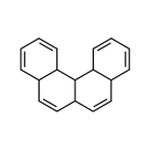
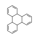
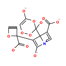
${\mathcal{T}}_{\textrm{4a}}$ (Kow)	${\mathcal{T}}_{\textrm{4b,0}}$ (Kow)	${\mathcal{T}}_{\textrm{4b,1}}$ (Kow)	${\mathcal{T}}_{\textrm{4b,2}}$ (Kow)

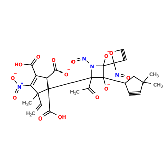
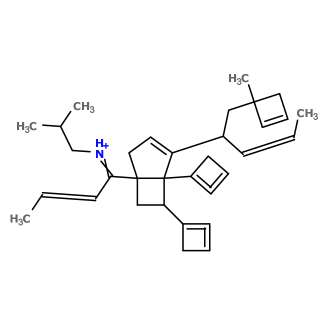
${\mathcal{T}}_{\textrm{4b,3}}$ (Kow)	${\mathcal{T}}_{5^{\ast}}$ (OptR)

Figure 4: Inferred chemical graphs

6 Concluding Remarks

In this paper, we proposed a new family of descriptors, cycle-configurations, that can be used in the standard 2L model of mol-infer. We introduced the definition in Section 3 and described how we deal with them in the MILP in Section 4. Then in Section 5, we demonstrated that the performance of a prediction function is improved in many cases when we introduce CC descriptors. We also showed that a chemical graph with up to 50 non-hydrogen atoms can be inferred in a practical time.

The 2L+CC model can be extended further in the similar way as the 2L model. Specifically, we can enumerate isomers of the inferred graph by dynamic programming [32] or generate “close” compounds in the sense of property values by a grid neighborhood approach [3]. Note that the constraint ${\mathcal{C}}_{1}$ of the MILP can contain multiple prediction functions for multiple properties, as is done in [31], where we have included a single property in this paper for simplicity. Besides, we may apply the 2L+CC model to inference of polymers. These are left for future work.

Appendix

Appendix A A Full Description of Descriptors in the 2L Model

Associated with the two functions $\alpha$ and $\beta$ in a chemical graph ${\mathbb{C}}=(H,\alpha,\beta)$, we introduce functions $\mathrm{ac}:V(E)\to(\Lambda\setminus\{{\mathtt{H}}\})\times(\Lambda\setminus\{{\mathtt{H}}\})\times[1,3]$, $\mathrm{cs}:V(E)\to(\Lambda\setminus\{{\mathtt{H}}\})\times[1,4]$ and $\mathrm{ec}:V(E)\to((\Lambda\setminus\{{\mathtt{H}}\})\times[1,4])\times((\Lambda\setminus\{{\mathtt{H}}\})\times[1,4])\times[1,3]$ in the following.

To represent a feature of the exterior of ${\mathbb{C}}$, a chemical rooted tree in $\mathcal{T}({\mathbb{C}})$ is called a fringe-configuration of ${\mathbb{C}}$.

We also represent leaf-edges in the exterior of ${\mathbb{C}}$. For a leaf-edge $uv\in E(\langle{\mathbb{C}}\rangle)$ with $\deg_{\langle{\mathbb{C}}\rangle}(u)=1$, we define the adjacency-configuration of $e$ to be an ordered tuple $(\alpha(u),\alpha(v),\beta(uv))$. Define

$$\Gamma_{\mathrm{ac}}^{\mathrm{lf}}\triangleq\{({\mathtt{a}},{\mathtt{b}},m)\mid{\mathtt{a}},{\mathtt{b}}\in\Lambda,m\in[1,\min\{\mathrm{val}({\mathtt{a}}),\mathrm{val}({\mathtt{b}})\}]\}$$

as a set of possible adjacency-configurations for leaf-edges.

To represent a feature of an interior-vertex $v\in V^{\mathrm{int}}({\mathbb{C}})$ such that $\alpha(v)={\mathtt{a}}$ and $\deg_{\langle{\mathbb{C}}\rangle}(v)=d$ (i.e., the number of non-hydrogen atoms adjacent to $v$ is $d$) in a chemical graph ${\mathbb{C}}=(H,\alpha,\beta)$, we use a pair $({\mathtt{a}},d)\in(\Lambda\setminus\{{\tt H}\})\times[1,4]$, which we call the chemical symbol $\mathrm{cs}(v)$ of the vertex $v$. We treat $({\mathtt{a}},d)$ as a single symbol ${\mathtt{a}}d$, and define $\Lambda_{\mathrm{dg}}$ to be the set of all chemical symbols $\mu={\mathtt{a}}d\in(\Lambda\setminus\{{\tt H}\})\times[1,4]$.

We define a method for featuring interior-edges as follows. Let $e=uv\in E^{\mathrm{int}}({\mathbb{C}})$ be an interior-edge $e=uv\in E^{\mathrm{int}}({\mathbb{C}})$ such that $\alpha(u)={\mathtt{a}}$, $\alpha(v)={\mathtt{b}}$ and $\beta(e)=m$ in a chemical graph ${\mathbb{C}}=(H,\alpha,\beta)$. To feature this edge $e$, we use a tuple $({\mathtt{a}},{\mathtt{b}},m)\in(\Lambda\setminus\{{\tt H}\})\times(\Lambda\setminus\{{\tt H}\})\times[1,3]$, which we call the adjacency-configuration $\mathrm{ac}(e)$ of the edge $e$. We introduce a total order $<$ over the elements in $\Lambda$ to distinguish between $({\mathtt{a}},{\mathtt{b}},m)$ and $({\mathtt{b}},{\mathtt{a}},m)$ $({\mathtt{a}}\neq{\mathtt{b}})$ notationally. For a tuple $\nu=({\mathtt{a}},{\mathtt{b}},m)$, let $\overline{\nu}$ denote the tuple $({\mathtt{b}},{\mathtt{a}},m)$.

Let $e=uv\in E^{\mathrm{int}}({\mathbb{C}})$ be an interior-edge $e=uv\in E^{\mathrm{int}}({\mathbb{C}})$ such that $\mathrm{cs}(u)=\mu$, $\mathrm{cs}(v)=\mu^{\prime}$ and $\beta(e)=m$ in a chemical graph ${\mathbb{C}}=(H,\alpha,\beta)$. To feature this edge $e$, we use a tuple $(\mu,\mu^{\prime},m)\in\Lambda_{\mathrm{dg}}\times\Lambda_{\mathrm{dg}}\times[1,3]$, which we call the edge-configuration $\mathrm{ec}(e)$ of the edge $e$. We introduce a total order $<$ over the elements in $\Lambda_{\mathrm{dg}}$ to distinguish between $(\mu,\mu^{\prime},m)$ and $(\mu^{\prime},\mu,m)$ $(\mu\neq\mu^{\prime})$ notationally. For a tuple $\gamma=(\mu,\mu^{\prime},m)$, let $\overline{\gamma}$ denote the tuple $(\mu^{\prime},\mu,m)$.

Let $\pi$ be a chemical property for which we will construct a prediction function $\eta$ from a feature vector $f({\mathbb{C}})$ of a chemical graph ${\mathbb{C}}$ to a predicted value $y\in\mathbb{R}$ for the chemical property of ${\mathbb{C}}$.

We first choose a set $\Lambda$ of chemical elements and then collect a data set $D_{\pi}$ of chemical compounds $C$ whose chemical elements belong to $\Lambda$, where we regard $D_{\pi}$ as a set of chemical graphs ${\mathbb{C}}$ that represent the chemical compounds $C$ in $D_{\pi}$. To define the interior/exterior of chemical graphs ${\mathbb{C}}\in D_{\pi}$, we next choose a branch-parameter ${\rho}$, where we recommend ${\rho}=2$.

Let $\Lambda^{\mathrm{int}}(D_{\pi})\subseteq\Lambda$ (resp., $\Lambda^{\mathrm{ex}}(D_{\pi})\subseteq\Lambda$) denote the set of chemical elements used in the set $V^{\mathrm{int}}({\mathbb{C}})$ of interior-vertices (resp., the set $V^{\mathrm{ex}}({\mathbb{C}})$ of exterior-vertices) of ${\mathbb{C}}$ over all chemical graphs ${\mathbb{C}}\in D_{\pi}$, and $\Gamma^{\mathrm{int}}(D_{\pi})$ denote the set of edge-configurations used in the set $E^{\mathrm{int}}({\mathbb{C}})$ of interior-edges in ${\mathbb{C}}$ over all chemical graphs ${\mathbb{C}}\in D_{\pi}$. Let $\mathcal{F}(D_{\pi})$ denote the set of chemical rooted trees $\psi$ r-isomorphic to a chemical rooted tree in $\mathcal{T}({\mathbb{C}})$ over all chemical graphs ${\mathbb{C}}\in D_{\pi}$, where possibly a chemical rooted tree $\psi\in\mathcal{F}(D_{\pi})$ consists of a single chemical element ${\mathtt{a}}\in\Lambda\setminus\{{\tt H}\}$.

We define an integer encoding of a finite set $A$ of elements to be a bijection $\pi:A\to[1,|A|]$, where we denote by $[A]$ the set $[1,|A|]$ of integers. Introduce an integer coding of each of the sets $\Lambda^{\mathrm{int}}(D_{\pi})$, $\Lambda^{\mathrm{ex}}(D_{\pi})$, $\Gamma^{\mathrm{int}}(D_{\pi})$ and $\mathcal{F}(D_{\pi})$. Let $[{\mathtt{a}}]^{\mathrm{int}}$ (resp., $[{\mathtt{a}}]^{\mathrm{ex}}$) denote the coded integer of an element ${\mathtt{a}}\in\Lambda^{\mathrm{int}}(D_{\pi})$ (resp., ${\mathtt{a}}\in\Lambda^{\mathrm{ex}}(D_{\pi})$), $[\gamma]$ denote the coded integer of an element $\gamma$ in $\Gamma^{\mathrm{int}}(D_{\pi})$ and $[\psi]$ denote an element $\psi$ in $\mathcal{F}(D_{\pi})$.

Over 99% of chemical compounds ${\mathbb{C}}$ with up to 100 non-hydrogen atoms in PubChem have degree at most 4 in the hydrogen-suppressed graph $\langle{\mathbb{C}}\rangle$ [5]. We assume that a chemical graph ${\mathbb{C}}$ treated in this paper satisfies $\deg_{\langle{\mathbb{C}}\rangle}(v)\leq 4$ in the hydrogen-suppressed graph $\langle{\mathbb{C}}\rangle$.

In our model, we use an integer $\mathrm{mass}^{*}({\mathtt{a}})=\lfloor 10\cdot\mathrm{mass}({\mathtt{a}})\rfloor$, for each ${\mathtt{a}}\in\Lambda$.

For a chemical property $\pi$, we define a set $D_{\pi}^{(1)}$ of descriptors of a chemical graph ${\mathbb{C}}=(H,\alpha,\beta)\in D_{\pi}$ to be the following non-negative values $\mathrm{dcp}_{i}({\mathbb{C}})$, $i\in[1,K_{\textrm{2L}}]$, where $K_{\textrm{2L}}=14+|\Lambda^{\mathrm{int}}(D_{\pi})|+|\Lambda^{\mathrm{ex}}(D_{\pi})|+|\Gamma^{\mathrm{int}}(D_{\pi})|+|\mathcal{F}(D_{\pi})|+|\Gamma_{\mathrm{ac}}^{\mathrm{lf}}|$.

1. $\mathrm{dcp}_{1}({\mathbb{C}})$: the number $|V(H)|-|V_{{\mathtt{H}}}|$ of non-hydrogen atoms in ${\mathbb{C}}$.

2. $\mathrm{dcp}_{2}({\mathbb{C}})$: the rank of ${\mathbb{C}}$ (i.e., the minimum number of edges to be removed to make the graph acyclic).

3. $\mathrm{dcp}_{3}({\mathbb{C}})$: the number $|V^{\mathrm{int}}({\mathbb{C}})|$ of interior-vertices in ${\mathbb{C}}$.

4. $\mathrm{dcp}_{4}({\mathbb{C}})$: the average $\overline{\mathrm{ms}}({\mathbb{C}})$ of mass^∗ over all atoms in ${\mathbb{C}}$;
   i.e., $\overline{\mathrm{ms}}({\mathbb{C}})\triangleq\frac{1}{|V(H)|}\sum_{v\in V(H)}\mathrm{mass}^{*}(\alpha(v))$.

5. $\mathrm{dcp}_{i}({\mathbb{C}})$, $i=4+d,d\in[1,4]$: the number $\mathrm{dg}_{d}^{\overline{{\tt H}}}({\mathbb{C}})$ of non-hydrogen vertices $v\in V(H)\setminus V_{{\mathtt{H}}}$ of degree $\deg_{\langle{\mathbb{C}}\rangle}(v)=d$ in the hydrogen-suppressed chemical graph $\langle{\mathbb{C}}\rangle$.

6. $\mathrm{dcp}_{i}({\mathbb{C}})$, $i=8+d,d\in[1,4]$: the number $\mathrm{dg}_{d}^{\mathrm{int}}({\mathbb{C}})$ of interior-vertices of interior-degree $\deg_{{\mathbb{C}}^{\mathrm{int}}}(v)=d$ in the interior ${\mathbb{C}}^{\mathrm{int}}=(V^{\mathrm{int}}({\mathbb{C}}),E^{\mathrm{int}}({\mathbb{C}}))$ of ${\mathbb{C}}$.

7. $\mathrm{dcp}_{i}({\mathbb{C}})$, $i=12+m$, $m\in[2,3]$: the number $\mathrm{bd}_{m}^{\mathrm{int}}({\mathbb{C}})$ of interior-edges with bond multiplicity $m$ in ${\mathbb{C}}$; i.e., $\mathrm{bd}_{m}^{\mathrm{int}}({\mathbb{C}})\triangleq|\{e\in E^{\mathrm{int}}({\mathbb{C}})\mid\beta(e)=m\}|$.

8. $\mathrm{dcp}_{i}({\mathbb{C}})$, $i=14+[{\mathtt{a}}]^{\mathrm{int}}$, ${\mathtt{a}}\in\Lambda^{\mathrm{int}}(D_{\pi})$: the frequency $\mathrm{na}_{\mathtt{a}}^{\mathrm{int}}({\mathbb{C}})=|V_{\mathtt{a}}({\mathbb{C}})\cap V^{\mathrm{int}}({\mathbb{C}})|$ of chemical element ${\mathtt{a}}$ in the set $V^{\mathrm{int}}({\mathbb{C}})$ of interior-vertices in ${\mathbb{C}}$.

9. $\mathrm{dcp}_{i}({\mathbb{C}})$, $i=14+|\Lambda^{\mathrm{int}}(D_{\pi})|+[{\mathtt{a}}]^{\mathrm{ex}}$, ${\mathtt{a}}\in\Lambda^{\mathrm{ex}}(D_{\pi})$: the frequency $\mathrm{na}_{\mathtt{a}}^{\mathrm{ex}}({\mathbb{C}})=|V_{\mathtt{a}}({\mathbb{C}})\cap V^{\mathrm{ex}}({\mathbb{C}})|$ of chemical element ${\mathtt{a}}$ in the set $V^{\mathrm{ex}}({\mathbb{C}})$ of exterior-vertices in ${\mathbb{C}}$.

10. $\mathrm{dcp}_{i}({\mathbb{C}})$, $i=14+|\Lambda^{\mathrm{int}}(D_{\pi})|+|\Lambda^{\mathrm{ex}}(D_{\pi})|+[\gamma]$, $\gamma\in\Gamma^{\mathrm{int}}(D_{\pi})$: the frequency $\mathrm{ec}_{\gamma}({\mathbb{C}})$ of edge-configuration $\gamma$ in the set $E^{\mathrm{int}}({\mathbb{C}})$ of interior-edges in ${\mathbb{C}}$.

11. $\mathrm{dcp}_{i}({\mathbb{C}})$, $i=14+|\Lambda^{\mathrm{int}}(D_{\pi})|+|\Lambda^{\mathrm{ex}}(D_{\pi})|+|\Gamma^{\mathrm{int}}(D_{\pi})|+[\psi]$, $\psi\in\mathcal{F}(D_{\pi})$: the frequency $\mathrm{fc}_{\psi}({\mathbb{C}})$ of fringe-configuration $\psi$ in the set of ${\rho}$-fringe-trees in ${\mathbb{C}}$.

12. $\mathrm{dcp}_{i}({\mathbb{C}})$, $i=14+|\Lambda^{\mathrm{int}}(D_{\pi})|+|\Lambda^{\mathrm{ex}}(D_{\pi})|+|\Gamma^{\mathrm{int}}(D_{\pi})|+|\mathcal{F}(D_{\pi})|+[\nu]$, $\nu\in\Gamma_{\mathrm{ac}}^{\mathrm{lf}}$: the frequency $\mathrm{ac}_{\nu}^{\mathrm{lf}}({\mathbb{C}})$ of adjacency-configuration $\nu$ in the set of leaf-edges in $\langle{\mathbb{C}}\rangle$.

Appendix B MILP Formulation for the 2L$+$CC Model

Let ${\mathcal{T}}=(T;V^{\circ},E^{\circ})$ denote a seed tree. Each ring node $u\in V^{\circ}$ is expanded to a cycle whose length is between $c_{\min}$ and $c_{\max}$. This expansion is done by assigning $\xi\in\Xi$ to $u$, where $\Xi^{u}$ is the set of cycle-configurations available to $u$ such that every $\xi\in\Xi$ satisfies $c_{\min}\leq|\xi|\leq c_{\max}$. Strictly speaking, a ring node $u\in V^{\circ}$ is assigned a graph $C^{u}$ such that $V(C^{u})=\{u_{1},u_{2},\dots,u_{c_{\max}}\}$ and $E(C^{u})=\{e^{u}_{1},e^{u}_{2},\dots,e^{u}_{2c_{\max}-c_{\min}}\}$, where, for $i\in[1,2c_{\max}-c_{\min}]$,

$$e^{u}_{i}=\left\{\begin{array}[]{ll}u_{i}u_{i+1}&\textrm{if\ }i\leq c_{\max},\\ u_{1}u_{i-c_{\max}+c_{\min}-1}&\textrm{otherwise},\end{array}\right.$$

and we regard $u_{c_{\max}+1}=u_{1}$ for convenience. The vertices and edges that form the cycle are chosen according to $|\xi|$, where $\xi$ is the cycle-configuration assigned to $u$. Specifically, vertices $u_{1},u_{2},\dots,u_{|\xi|}$ and edges $u_{1}u_{2},\dots,u_{|\xi|-1}u_{|\xi|},u_{|\xi|}u_{1}$ are chosen.

For a cycle-configuration $\xi$ and $r\in[1,c_{\max}]$, let us define

$$\hat{\xi}^{+}(r)\triangleq\{(\mu,\mu_{0})\mid\mu,\mu_{0}\in\{u_{1},\dots,u_{|\xi|}\},\ \xi(\mu-\mu_{0}+1)=r\};$$

$$\hat{\xi}^{-}(r)\triangleq\{(\mu,\mu_{0})\mid\mu,\mu_{0}\in\{u_{1},\dots,u_{|\xi|}\},\ \xi(\mu_{0}-\mu+1)=r\},$$

and for $\mu\in V(C^{u})$ and $\delta\in\{+,-\}$, we let

$$\hat{\xi}^{\delta}(r,\mu):=\{\mu_{0}\in V(C^{u})\mid(\mu,\mu_{0})\in\hat{\xi}^{\delta}(r)\}.$$

B.1 Assigning Cycle-Configurations to Ring Nodes

Constants.

• A seed tree ${\mathcal{T}}=(T;V^{\circ},E^{\circ})$;

• the set $\Xi^{u}$ of available cycle-configurations for each $u\in V^{\circ}$, $\Xi^{\mathcal{T}}:=\bigcup_{u\in V^{\circ}}\Xi^{u}$;

• a positive constant $\varepsilon_{1}\in\mathbb{R}_{+}$ that represents a sufficiently small number;

• a positive constant $M_{1}\in\mathbb{R}_{+}$ that represents a sufficiently large number.

Variables.

• Real variables $y^{u}_{[\mu]}$, $u\in V^{\circ}$, $\mu\in V(C^{u})$ that store the mass sum in the fringe-tree attached to vertex $\mu\in V(C^{u})$;

• real variables $z^{u}_{r}$, $u\in V^{\circ}$, $r\in[1,c_{\max}]$ that represent the $r$-th smallest mass sum of a fringe-tree in $C^{u}$;

• binary variables $x^{u}_{[\xi],[\mu_{0}],\delta}$, $u\in V^{\circ}$, $\xi\in\Xi^{u}$, $\mu_{0}\in\{u_{1},\dots,u_{|\xi|}\}$ and $\delta\in\{+,-\}$, indicating whether $\xi$ is assigned to the starting point $\mu_{0}$ in the direction $\delta$;

• binary variables $x_{[\xi]}^{u}$, $u\in V^{\circ}$, $\xi\in\Xi^{u}$, indicating whether $\xi$ is assigned to $C^{u}$;

• integer variables ${\mathrm{cc}}([\xi])$, $\xi\in\Xi^{\mathcal{T}}$, cycle-configurations.

Constraints.

For each $u\in V^{\circ}$:

$$0\leq z^{u}_{1},\dots,z^{u}_{c_{\max}}\leq M_{1},$$ (1)

$$z^{u}_{r}+\varepsilon_{1}\leq z^{u}_{r+1}, r\in[1,c_{\max}-1];$$ (2)

$$x_{[\xi]}^{u}=\sum_{\mu_{0}\in\{u_{1},\dots,u_{|\xi|}\}}\sum_{\delta\in\{+,-\}}x_{[\xi],[\mu_{0}],\delta}^{u}, \xi\in\Xi^{u};$$ (3)

$$\sum_{\xi\in\Xi^{u}}x_{[\xi]}^{u}=1;$$ (4)

$$y^{u}_{[\mu]}\leq z^{u}_{r}+M_{1}\big{(}1-\sum_{\xi\in\Xi^{u}}\sum_{\delta\in\{+,-\}}\sum_{\mu_{0}\in\hat{\xi}^{\delta}(r,\mu)}x^{u}_{[\xi],[\mu_{0}],\delta}\big{)}, r\in[1,c_{\max}],\ \mu\in V(C^{u});$$ (5)

$$y^{u}_{[\mu]}\geq z^{u}_{r}-M_{1}\big{(}1-\sum_{\xi\in\Xi^{u}}\sum_{\delta\in\{+,-\}}\sum_{\mu_{0}\in\hat{\xi}^{\delta}(r,\mu)}x^{u}_{[\xi],[\mu_{0}],\delta}\big{)}, r\in[1,c_{\max}],\ \mu\in V(C^{u}).$$ (6)

For each $\xi\in\Xi^{\mathcal{T}}$:

$${\mathrm{cc}}([\xi])=\sum_{u\in V^{\circ},\xi\in\Xi^{u}}x_{[\xi]}^{u},$$ (7)

B.2 Associating Ring Nodes with Ring Edges

Variables.

• Binary variables $e_{i}^{u},u\in V^{\circ},i\in[1,2c_{\max}-c_{\min}]$, indicating whether the edge $e_{i}$ in $C^{u}$ is used;

• binary variables $x^{{\rm edge},u}_{[e],[\nu]}$, $u\in V^{\circ}$, $e\in E^{\circ}(u)$, $\nu\in E(C^{u})$;

• binary variables $x^{{\rm node},u}_{[e^{\prime}],[\mu]}$, $u\in V^{\circ}$, $e^{\prime}\in\bar{E}^{\circ}(u)$, $\mu\in V(C^{u})$;

Constraints.

For each $u\in V^{\circ}$:

$$\sum_{\nu\in E(C^{u})}x^{{\rm edge},u}_{[e],[\nu]}=1, e\in E^{\circ}(u);$$ (8)

$$\sum_{\mu\in V(C^{u})}x^{{\rm node},u}_{[e^{\prime}],[\mu]}=1, e^{\prime}\in\bar{E}^{\circ}(u);$$ (9)

$$\sum_{e\in E^{\circ}(u)}\sum_{\nu\in(E(C^{u}))(\mu)}x_{[e],[\nu]}^{{\rm edge},u}\leq 1, \mu\in V(C^{u});$$ (10)

$$\sum_{e\in E^{\circ}(u)}x_{[e],[\nu]}^{{\rm edge},u}\leq 1, \nu\in E(C^{u});$$ (11)

For each $u\in V^{\circ}$:

$$e_{i}^{u}=1, i\in[1,c_{\min}-1];$$

$$e_{i}^{u}=\sum_{\xi\in\Xi^{u},|\xi|>i}x_{[\xi]}^{u}, i\in[c_{\min},c_{\max}-2];$$

$$e_{i}^{u}=\sum_{\xi\in\Xi^{u},|\xi|=c_{\max}}x_{[\xi]}^{u}, i\in\{c_{\max}-1,c_{\max}\};$$

$$e_{i}^{u}=\sum_{\xi\in\Xi^{u},|\xi|=i-c_{\max}+c_{\min}-1}x_{[\xi]}^{u}, i\in[c_{\max}+1,2c_{\max}-c_{\min}];$$ (12)

$$x_{[e],i}^{{\rm edge},u}\leq e_{i}^{u}, e\in E^{\circ}(u),i\in[1,2c_{\max}-c_{\min}];$$ (13)

$$x_{[e^{\prime}],i}^{{\rm node},u}\leq\sum_{\xi\in\Xi^{u},|\xi|\geq i}x_{[\xi]}^{u}, e^{\prime}\in\bar{E}^{\circ}(u),i\in[c_{\min}+1,c_{\max}];$$ (14)

B.3 Constraints for Including Fringe-Trees

For a leaf-edge $uv\in E(G_{\mathcal{T}})$ with $\deg_{G_{\mathcal{T}}}(u)=1$, we define the adjacency-configuration of $uv$ to be an ordered tuple $(\alpha(u),\alpha(v),\beta(uv))$.

Constants.

• The set ${\mathcal{F}}^{u}$ of the available fringe-trees for each $u\in V(T)$, ${\mathcal{F}}^{\mathcal{T}}:=\bigcup_{u\in V(T)}{\mathcal{F}}^{u}$;

• the set ${\Gamma_{\mathrm{ac}}^{\mathrm{lf}}}$ of available adjacency-configuration on the set of leaf-edges;

• functions ${\mathrm{ms}_{\mathcal{F}}}(\psi),{\mathrm{ht}_{\mathcal{F}}}(\psi),{n_{\overline{{\mathtt{H}}}}}(\psi),{\mathrm{ac}_{\gamma}^{\mathrm{lf}}}(\psi)$ denoting the mass, height, number of non-hydrogen non-root atoms, number of leaf-edge adjacency-configurations $\gamma$ of the fringe-tree $\psi$, respectively;

• integers ${n_{\mathrm{LB}}},{n_{\mathrm{UB}}}$, that represent the lower and upper bounds on the number of non-hydrogen atoms in $G_{\mathcal{T}}$, respectively;

• integers ${n^{\mathrm{int}}_{\mathrm{LB}}},{n^{\mathrm{int}}_{\mathrm{UB}}}$, that represent the lower and upper bounds on the number of non-hydrogen atoms in the interior part of $G_{\mathcal{T}}$, respectively;

• integers ${\mathrm{fc}_{\mathrm{LB}}}(\psi),{\mathrm{fc}_{\mathrm{UB}}}(\psi)\in[0,{n_{\mathrm{UB}}}],\psi\in{\mathcal{F}}^{\mathcal{T}}$, that represent the lower and upper bounds on the fringe-configurations, respectively;

• integers ${\mathrm{ac}^{\mathrm{lf}}_{\mathrm{LB}}}(\gamma),{\mathrm{ac}^{\mathrm{lf}}_{\mathrm{UB}}}(\gamma)\in[0,{n_{\mathrm{UB}}}],\gamma\in{\Gamma_{\mathrm{ac}}^{\mathrm{lf}}}$, that represent the lower and upper bounds on the adjacency-configurations of leaf-edges, respectively;

Variables.

• Binary variables $\delta_{\mathcal{F}}(u,[\mu];[\psi])$, $u\in V^{\circ},\mu\in V(C^{u})$, $\psi\in{\mathcal{F}}^{u}$, indicating whether the fringe-tree $\psi$ is attached to vertex $\mu\in V(C^{u})$;

• binary variables $\delta_{\mathcal{F}}(v;[\psi])$, $v\in V(T)\setminus V^{\circ}$, $\psi\in{\mathcal{F}}^{v}$, indicating whether the fringe-tree $\psi$ is attached to node $v\in V(T)\setminus V^{\circ}$;

• integer variables $\mathrm{fc}([e];[\psi])\in[0,2]$, $e\in E^{\circ}$, $\psi\in{\mathcal{F}}^{\mathcal{T}}$, that stores the number of the fringe-tree $\psi$ is used in the ring edge $e\in E^{\circ}$;

• integer variable $\mathrm{rank}$ that represents the rank of $G_{\mathcal{T}}$;

• integer variables $n_{G}\in[{n_{\mathrm{LB}}},{n_{\mathrm{UB}}}],{n_{\mathrm{int}}}\in[{n^{\mathrm{int}}_{\mathrm{LB}}},{n^{\mathrm{int}}_{\mathrm{UB}}}]$ that represents the number of non-hydrogen atoms in $G_{\mathcal{T}}$ and the interior part of $G_{\mathcal{T}}$, respectively;

• integer variables $\mathrm{fc}([\psi])\in[{\mathrm{fc}_{\mathrm{LB}}}(\psi),{\mathrm{fc}_{\mathrm{UB}}}(\psi)]$, $\psi\in{\mathcal{F}}^{\mathcal{T}}$ that stores the fringe-configurations;

• integer variables ${\mathrm{ac}^{\mathrm{lf}}}([\gamma])\in[{\mathrm{ac}^{\mathrm{lf}}_{\mathrm{LB}}}(\gamma),{\mathrm{ac}^{\mathrm{lf}}_{\mathrm{UB}}}(\gamma)]$, $\gamma\in{\Gamma_{\mathrm{ac}}^{\mathrm{lf}}}$, that stores the adjacency-configurations of leaf-edges;

Constraints.

For each $u\in V^{\circ},\mu\in V(C^{u})$:

$$\sum_{\psi\in{\mathcal{F}}^{u}}\delta_{\mathcal{F}}(u,[\mu];[\psi])=\sum_{\xi\in\Xi^{u},|\xi|\geq[\mu]}x_{[\xi]}^{u};$$ (15)

$$\sum_{\psi\in{\mathcal{F}}^{u}}{\mathrm{ms}_{\mathcal{F}}}(\psi)\cdot\delta_{\mathcal{F}}(u,[\mu];[\psi])=y_{[\mu]}^{u};$$ (16)

For each $v\in V(T)\setminus V^{\circ}$:

$$\sum_{\psi\in{\mathcal{F}}^{v}}\delta_{\mathcal{F}}(v;[\psi])=1,$$

$$\sum_{\psi\in{\mathcal{F}}^{v},{\mathrm{ht}_{\mathcal{F}}}(\psi)=\rho}\delta_{\mathcal{F}}(v;[\psi])=1, v\ \textrm{is\ a\ leaf\ of}\ T;$$ (17)

For each $e=uu^{\prime}\in E^{\circ}$ such that $[u]<[u^{\prime}]$:

$$\sum_{\psi\in{\mathcal{F}}^{u}}[\psi]\cdot\delta_{\mathcal{F}}(u,i_{1};[\psi])-\sum_{\psi\in{\mathcal{F}}^{u^{\prime}}}[\psi]\cdot\delta_{\mathcal{F}}(u^{\prime},j_{2};[\psi])\leq |{\mathcal{F}}^{\mathcal{T}}|(2-x^{{\rm edge},u}_{[e],[\nu]}-x^{{\rm edge},u^{\prime}}_{[e],[\nu^{\prime}]}),$$

$$\sum_{\psi\in{\mathcal{F}}^{u}}[\psi]\cdot\delta_{\mathcal{F}}(u,i_{1};[\psi])-\sum_{\psi\in{\mathcal{F}}^{u^{\prime}}}[\psi]\cdot\delta_{\mathcal{F}}(u^{\prime},j_{2};[\psi])\geq |{\mathcal{F}}^{\mathcal{T}}|(x^{{\rm edge},u}_{[e],[\nu]}+x^{{\rm edge},u^{\prime}}_{[e],[\nu^{\prime}]}-2),$$

$$\sum_{\psi\in{\mathcal{F}}^{u}}[\psi]\cdot\delta_{\mathcal{F}}(u,i_{2};[\psi])-\sum_{\psi\in{\mathcal{F}}^{u^{\prime}}}[\psi]\cdot\delta_{\mathcal{F}}(u^{\prime},j_{1};[\psi])\leq |{\mathcal{F}}^{\mathcal{T}}|(2-x^{{\rm edge},u}_{[e],[\nu]}-x^{{\rm edge},u^{\prime}}_{[e],[\nu^{\prime}]}),$$

$$\sum_{\psi\in{\mathcal{F}}^{u}}[\psi]\cdot\delta_{\mathcal{F}}(u,i_{2};[\psi])-\sum_{\psi\in{\mathcal{F}}^{u^{\prime}}}[\psi]\cdot\delta_{\mathcal{F}}(u^{\prime},j_{1};[\psi])\geq |{\mathcal{F}}^{\mathcal{T}}|(x^{{\rm edge},u}_{[e],[\nu]}+x^{{\rm edge},u^{\prime}}_{[e],[\nu^{\prime}]}-2),$$

$$\nu=u_{i_{1}}u_{i_{2}}\in E(C^{u}),\ \nu^{\prime}=u^{\prime}_{j_{1}}u^{\prime}_{j_{2}}\in E(C^{u^{\prime}})$$

$$\textrm{such\ that\ }i_{1}<i_{2},\ j_{1}<j_{2};$$ (18)

$$\mathrm{fc}([e];[\psi])-\delta_{\mathcal{F}}(u,i_{1};[\psi])-\delta_{\mathcal{F}}(u,i_{2};[\psi])\leq 2(1-x_{[e],[\nu]}^{{\rm edge},u}),$$

$$\mathrm{fc}([e];[\psi])-\delta_{\mathcal{F}}(u,i_{1};[\psi])-\delta_{\mathcal{F}}(u,i_{2};[\psi])\geq 2(x_{[e],[\nu]}^{{\rm edge},u}-1), \nu=u_{i_{1}}u_{i_{2}}\in E(C^{u}),\psi\in{\mathcal{F}}^{\mathcal{T}};$$ (19)

For each $\psi\in{\mathcal{F}}^{\mathcal{T}}$:

$$\mathrm{fc}([\psi])=\sum_{u\in V^{\circ}}\sum_{\mu\in V(C^{u})}\delta_{\mathcal{F}}(u,[\mu];[\psi])+\sum_{v\in V(T)\setminus V^{\circ}}\delta_{\mathcal{F}}(v;[\psi])-\sum_{e\in E^{\circ}}\mathrm{fc}([e];[\psi]);$$ (20)

For each $\gamma\in{\Gamma_{\mathrm{ac}}^{\mathrm{lf}}}$:

$${\mathrm{ac}^{\mathrm{lf}}}([\gamma])=\sum_{\psi\in{\mathcal{F}}^{\mathcal{T}}}{\mathrm{ac}_{\gamma}^{\mathrm{lf}}}(\psi)\mathrm{fc}([\psi]);$$ (21)

$$\mathrm{rank}=|V^{\circ}|;$$ (22)

$${n_{\mathrm{int}}}=\sum_{u\in V^{\circ}}\sum_{\xi\in\Xi^{u}}|\xi|\cdot x_{[\xi]}^{u}+|V(T)\setminus V^{\circ}|-2|E^{\circ}|;$$ (23)

$$n_{G}={n_{\mathrm{int}}}+\sum_{\psi\in{\mathcal{F}}^{\mathcal{T}}}{n_{\overline{{\mathtt{H}}}}}(\psi)\mathrm{fc}([\psi]);$$ (24)

B.4 Descriptors for the Number of Specified Degree

Constants.

• Function ${\mathrm{deg}_{\overline{{\mathtt{H}}}}}(\psi)$ denoting the degree of the root of the fringe tree $\psi$;

Variables.

• Binary variables ${\delta_{\mathrm{deg}}}(u,[\mu];d),u\in V^{\circ},\mu\in V(C^{u}),d\in[1,4]$, indicating the degree of $\mu$ in $G_{{\mathcal{T}}}$;

• binary variables ${\delta_{\mathrm{deg}}}(v;d),v\in V(T)\setminus V^{\circ},d\in[1,4]$, indicating the degree of $v$ in $G_{{\mathcal{T}}}$;

• binary variables ${\delta^{\mathrm{int}}_{\mathrm{deg}}}(u,[\mu];d),u\in V^{\circ},\mu\in V(C^{u}),d\in[1,4]$, indicating the interior degree of $\mu$ in $G_{{\mathcal{T}}}$;

• binary variables ${\delta^{\mathrm{int}}_{\mathrm{deg}}}(v;d),v\in V(T)\setminus V^{\circ},d\in[1,4]$, indicating the interior degree of $v$ in $G_{{\mathcal{T}}}$;

• integer variables $\mathrm{dg}(d),d\in[1,4]$, that stores the number of vertices with degree $d$ in $G_{\mathcal{T}}$;

• integer variables ${\mathrm{deg}^{\mathrm{int}}}(d),d\in[1,4]$, that stores the number of vertices with interior degree $d$ in $G_{\mathcal{T}}$;

• integer variables $\mathrm{dg}([e];d)\in[0,2],e\in E^{\circ},d\in[1,4]$, that stores the number of vertices with degree $d$ in the ring edge $e$;

• integer variables ${\mathrm{deg}^{\mathrm{int}}}([e];d)\in[0,2],e\in E^{\circ},d\in[1,4]$, that stores the number of vertices with interior degree $d$ in the ring edge $e$;

• integer variables $\mathrm{dg}_{[e],[\mu],+}^{{\rm edge},u},u\in V^{\circ},\mu\in V(C^{u}),e\in E^{\circ}(u)$, indicating the degree other than that of the ring edge $e$ at $\mu$ in $C^{u}$;

• integer variables $\mathrm{dg}_{[e],[\mu],-}^{{\rm edge},u},u\in V^{\circ},\mu\in V(C^{u}),e\in E^{\circ}(u)$, indicating the augmented degree for $\mu$ because of the ring edge $e$;

Constraints.

For each $u\in V^{\circ},\mu\in V(C^{u})$:

$$0\leq\mathrm{dg}_{[e],[\mu],+}^{{\rm edge},u}\leq 4\sum_{\nu\in(E(C^{u}))(\mu)}x_{[e],[\nu]}^{{\rm edge},u} e\in E^{\circ}(u);$$

$$0\leq\mathrm{dg}_{[e],[\mu],-}^{{\rm edge},u}\leq 4\sum_{\nu\in(E(C^{u}))(\mu)}x_{[e],[\nu]}^{{\rm edge},u} e\in E^{\circ}(u);$$ (25)

$$4(x_{[e],[\nu]}^{{\rm edge},u}-1)\leq\mathrm{dg}_{[e],[\mu],+}^{{\rm edge},u}-1-\sum_{e^{\prime}\in\bar{E}^{\circ}(u)}x_{[e^{\prime}],[\mu]}^{{\rm node},u}\leq 4(1-x_{[e],[\nu]}^{{\rm edge},u}), e\in E^{\circ}(u),\nu\in(E(C^{u}))(\mu);$$ (26)

For each $e=uu^{\prime}\in E^{\circ}$ such that $[u]<[u^{\prime}]$:

$$3(x_{[e],[\nu]}^{{\rm edge},u}+x_{[e],[\nu^{\prime}]}^{{\rm edge},u^{\prime}}-2)\leq\mathrm{dg}_{[e],i_{1},-}^{{\rm edge},u}-\mathrm{dg}_{[e],j_{2},+}^{{\rm edge},u^{\prime}}\leq 3(2-x_{[e],[\nu]}^{{\rm edge},u}-x_{[e],[\nu^{\prime}]}^{{\rm edge},u^{\prime}}),$$

$$3(x_{[e],[\nu]}^{{\rm edge},u}+x_{[e],[\nu^{\prime}]}^{{\rm edge},u^{\prime}}-2)\leq\mathrm{dg}_{[e],i_{2},-}^{{\rm edge},u}-\mathrm{dg}_{[e],j_{1},+}^{{\rm edge},u^{\prime}}\leq 3(2-x_{[e],[\nu]}^{{\rm edge},u}-x_{[e],[\nu^{\prime}]}^{{\rm edge},u^{\prime}}),$$

$$3(x_{[e],[\nu]}^{{\rm edge},u}+x_{[e],[\nu^{\prime}]}^{{\rm edge},u^{\prime}}-2)\leq\mathrm{dg}_{[e],j_{2},-}^{{\rm edge},u^{\prime}}-\mathrm{dg}_{[e],i_{1},+}^{{\rm edge},u}\leq 3(2-x_{[e],[\nu]}^{{\rm edge},u}-x_{[e],[\nu^{\prime}]}^{{\rm edge},u^{\prime}}),$$

$$3(x_{[e],[\nu]}^{{\rm edge},u}+x_{[e],[\nu^{\prime}]}^{{\rm edge},u^{\prime}}-2)\leq\mathrm{dg}_{[e],j_{1},-}^{{\rm edge},u^{\prime}}-\mathrm{dg}_{[e],i_{2},+}^{{\rm edge},u}\leq 3(2-x_{[e],[\nu]}^{{\rm edge},u}-x_{[e],[\nu^{\prime}]}^{{\rm edge},u^{\prime}}),$$

$$\nu=u_{i_{1}}u_{i_{2}}\in E(C^{u}),\ \nu^{\prime}=u^{\prime}_{j_{1}}u^{\prime}_{j_{2}}\in E(C^{u^{\prime}})$$

$$\textrm{such\ that\ }i_{1}<i_{2},\ j_{1}<j_{2};$$ (27)

For each $u\in V^{\circ},\mu\in V(C^{u})$:

$$\sum_{d\in[1,4]}{\delta_{\mathrm{deg}}}(u,[\mu];d) =\sum_{\xi\in\Xi^{u},|\xi|\geq[\mu]}x_{[\xi]}^{u};$$ (28)

$$2(\sum_{\xi\in\Xi^{u},|\xi|\geq[\mu]}x_{[\xi]}^{u}-1) \leq\sum_{d\in[1,4]}d\cdot{\delta_{\mathrm{deg}}}(u,[\mu];d)-$$

$$(2+\sum_{\psi\in{\mathcal{F}}^{u}}{\mathrm{deg}_{\overline{{\mathtt{H}}}}}(\psi)\delta_{\mathcal{F}}(u,[\mu];[\psi])+\sum_{e^{\prime}\in\bar{E}^{\circ}(u)}x_{[e^{\prime}],[\mu]}^{{\rm node},u}+\sum_{e\in E^{\circ}(u)}\mathrm{dg}_{[e],[\mu],-}^{{\rm edge},u});$$

$$\sum_{d\in[1,4]}d\cdot{\delta_{\mathrm{deg}}}(u,[\mu];d) \leq\ 2+\sum_{\psi\in{\mathcal{F}}^{u}}{\mathrm{deg}_{\overline{{\mathtt{H}}}}}(\psi)\delta_{\mathcal{F}}(u,[\mu];[\psi])$$

$$+\sum_{e^{\prime}\in\bar{E}^{\circ}(u)}x_{[e^{\prime}],[\mu]}^{{\rm node},u}+\sum_{e\in E^{\circ}(u)}\mathrm{dg}_{[e],[\mu],-}^{{\rm edge},u});$$ (29)

$$\sum_{d\in[1,4]}{\delta^{\mathrm{int}}_{\mathrm{deg}}}(u,[\mu];d) =\sum_{\xi\in\Xi^{u},|\xi|\geq[\mu]}x_{[\xi]}^{u};$$ (30)

$$2(\sum_{\xi\in\Xi^{u},|\xi|\geq[\mu]}x_{[\xi]}^{u}-1) \leq\sum_{d\in[1,4]}d\cdot{\delta^{\mathrm{int}}_{\mathrm{deg}}}(u,[\mu];d)-\ (2+\sum_{e^{\prime}\in\bar{E}^{\circ}(u)}x_{[e^{\prime}],[\mu]}^{{\rm node},u}+\sum_{e\in E^{\circ}(u)}\mathrm{dg}_{[e],[\mu],-}^{{\rm edge},u});$$

$$\sum_{d\in[1,4]}d\cdot{\delta^{\mathrm{int}}_{\mathrm{deg}}}(u,[\mu];d) \leq\ 2+\sum_{e^{\prime}\in\bar{E}^{\circ}(u)}x_{[e^{\prime}],[\mu]}^{{\rm node},u}+\sum_{e\in E^{\circ}(u)}\mathrm{dg}_{[e],[\mu],-}^{{\rm edge},u});$$ (31)

For each $v\in V(T)\setminus V^{\circ}$:

$$\sum_{d\in[1,4]}{\delta_{\mathrm{deg}}}(v;d)=1;$$ (32)

$$\sum_{d\in[1,4]}d\cdot{\delta_{\mathrm{deg}}}(v;d)=|N_{T}(v)|+\sum_{\psi\in{\mathcal{F}}^{v}}{\mathrm{deg}_{\overline{{\mathtt{H}}}}}(\psi)\delta_{\mathcal{F}}(v;[\psi]);$$ (33)

$$\sum_{d\in[1,4]}{\delta^{\mathrm{int}}_{\mathrm{deg}}}(v;d)=1;$$ (34)

$$\sum_{d\in[1,4]}d\cdot{\delta^{\mathrm{int}}_{\mathrm{deg}}}(v;d)=|N_{T}(v)|;$$ (35)

For each $e=uu^{\prime}\in E^{\circ}$ such that $[u]<[u^{\prime}]$:

$$\mathrm{dg}([e];d)-{\delta_{\mathrm{deg}}}(u,i_{1};d)-{\delta_{\mathrm{deg}}}(u,i_{2};d)\leq 2(1-x_{[e],[\nu]}^{{\rm edge},u}),$$

$$\mathrm{dg}([e];d)-{\delta_{\mathrm{deg}}}(u,i_{1};d)-{\delta_{\mathrm{deg}}}(u,i_{2};d)\geq 2(x_{[e],[\nu]}^{{\rm edge},u}-1), \nu=u_{i_{1}}u_{i_{2}}\in E(C^{u}),d\in[1,4]$$ (36)

$${\mathrm{deg}^{\mathrm{int}}}([e];d)-{\delta^{\mathrm{int}}_{\mathrm{deg}}}(u,i_{1};d)-{\delta^{\mathrm{int}}_{\mathrm{deg}}}(u,i_{2};d)\leq 2(1-x_{[e],[\nu]}^{{\rm edge},u}),$$

$${\mathrm{deg}^{\mathrm{int}}}([e];d)-{\delta^{\mathrm{int}}_{\mathrm{deg}}}(u,i_{1};d)-{\delta^{\mathrm{int}}_{\mathrm{deg}}}(u,i_{2};d)\geq 2(x_{[e],[\nu]}^{{\rm edge},u}-1), \nu=u_{i_{1}}u_{i_{2}}\in E(C^{u}),d\in[1,4]$$ (37)

For each $d\in[1,4]$:

$$\mathrm{dg}(d)=\sum_{u\in V^{\circ}}\sum_{\mu\in V(C^{u})}{\delta_{\mathrm{deg}}}(u,[\mu];d)+\sum_{v\in V(T)\setminus V^{\circ}}{\delta_{\mathrm{deg}}}(v;d)-\sum_{e\in E^{\circ}}\mathrm{dg}([e];d);$$ (38)

$${\mathrm{deg}^{\mathrm{int}}}(d)=\sum_{u\in V^{\circ}}\sum_{\mu\in V(C^{u})}{\delta^{\mathrm{int}}_{\mathrm{deg}}}(u,[\mu];d)+\sum_{v\in V(T)\setminus V^{\circ}}{\delta^{\mathrm{int}}_{\mathrm{deg}}}(v;d)-\sum_{e\in E^{\circ}}{\mathrm{deg}^{\mathrm{int}}}([e];d);$$ (39)

B.5 Assigning Bond-Multiplicity

Variables.

• Integer variables $\beta_{i}^{u}\in[0,3],u\in V^{\circ},i\in[1,2c_{\max}-c_{\min}]$, that stores the bond-multiplicty of the edge $e_{i}$ in $C^{u}$;

• integer variables $\beta_{[e]}\in[1,3],e\in E(T)$, that stores the bond-multiplicty of the edge $e$;

• binary variables ${\delta_{\beta}}(u,i;m),u\in V^{\circ},i\in[1,2c_{\max}-c_{\min}],m\in[1,3]$, ${\delta_{\beta}}(u,i;m)=1\Leftrightarrow\beta_{i}^{u}=m$;

• binary variables ${\delta_{\beta}}([e];m),e\in E(T),m\in[1,3]$, ${\delta_{\beta}}([e];m)=1\Leftrightarrow\beta_{[e]}=m$;

• integer variables $\mathrm{bd}(m),m\in[1,3]$, that stores the number of edges with bond-multiplicty $m$;

Constraints.

$$e_{i}^{u}\leq\beta_{i}^{u}\leq 3e_{i}^{u}, u\in V^{\circ},i\in[1,2c_{\max}-c_{\min}];$$ (40)

$$1\leq\beta_{[e]}\leq 3, e\in E(T);$$ (41)

$$\sum_{m\in[1,3]}{\delta_{\beta}}(u,i;m)=e_{i}^{u}, \sum_{m\in[1,3]}m\cdot{\delta_{\beta}}(u,i;m)=\beta_{i}^{u}, u\in V^{\circ},i\in[1,2c_{\max}-c_{\min}];$$ (42)

$$\sum_{m\in[1,3]}{\delta_{\beta}}([e];m)=1, \sum_{m\in[1,3]}m\cdot{\delta_{\beta}}([e];m)=\beta_{[e]}, e\in E(T);$$ (43)

For each $u\in V^{\circ},e\in E^{\circ}(u)$:

$$3(x_{[e],i}^{{\rm edge},u}-1)\leq\beta_{i}^{u}-\beta_{[e]}\leq 3(1-x_{[e],i}^{{\rm edge},u}), i\in[1,2c_{\max}-c_{\min}];$$ (44)

For each $m\in[1,3]$:

$$\mathrm{bd}(m)=\sum_{u\in V^{\circ}}\sum_{i\in[1,2c_{\max}-c_{\min}]}{\delta_{\beta}}(u,i;m)+\sum_{e^{\prime}\in E(T)\setminus E^{\circ}}{\delta_{\beta}}([e^{\prime}];m)-\sum_{e\in E^{\circ}}{\delta_{\beta}}([e];m);$$ (45)

B.6 Assigning Chemical Elements and Valence Condition

Constants.

• A set $\Lambda$ consisting of all available chemical elements;

• functions ${\alpha_{\mathrm{r}}}(\psi),\mathrm{val}_{\mathcal{F}}^{\mathrm{ex}}(\psi),\mathrm{eledeg}_{\mathcal{F}}(\psi),{n_{{\mathtt{a}}}}(\psi)$ denoting the chemical element of the root, root valence, ion-valence, number of non-root chemical element ${\mathtt{a}}$ of the fringe-tree $\psi$, respectively;

• functions $\mathrm{val}({\mathtt{a}}),\mathrm{mass}^{*}({\mathtt{a}})$ denoting the valence and mass of the chemical element ${\mathtt{a}}$, respectively;

• integers ${\mathrm{na}^{\mathrm{int}}_{\mathrm{LB}}}([{\mathtt{a}}]),{\mathrm{na}^{\mathrm{int}}_{\mathrm{UB}}}([{\mathtt{a}}])\in[0,{n_{\mathrm{UB}}}],{\mathtt{a}}\in\Lambda$, that represent the lower and upper bounds of the chemical element ${\mathtt{a}}$ in the interior part, respectively;

• integers ${\mathrm{na}^{\mathrm{ex}}_{\mathrm{LB}}}([{\mathtt{a}}]),{\mathrm{na}^{\mathrm{ex}}_{\mathrm{UB}}}([{\mathtt{a}}])\in[0,{n_{\mathrm{UB}}}],{\mathtt{a}}\in\Lambda$, that represent the lower and upper bounds of the chemical element ${\mathtt{a}}$ in the exterior part, respectively;

• integers ${\mathrm{na}_{\mathrm{LB}}}([{\mathtt{a}}]),{\mathrm{na}_{\mathrm{UB}}}([{\mathtt{a}}])\in[0,{n_{\mathrm{UB}}}],{\mathtt{a}}\in\Lambda$, that represent the lower and upper bounds of the chemical element ${\mathtt{a}}$ in $G_{\mathcal{T}}$, respectively;

• a positive constant $M_{\mathrm{ms}}\in\mathbb{R}_{+}$ that represents a sufficiently large number;

Variables.

• Integer variables $\alpha(u,[\mu]),u\in V^{\circ},\mu\in V(C^{u})$, that represents the chemical element assigned to the vertex $\mu$ in $C^{u}$;

• integer variables $\alpha(v),v\in V(T)\setminus V^{\circ}$, that represents the chemical element assigned to the vertex $v$;

• binary variables ${\delta_{\alpha}}(u,[\mu];[{\mathtt{a}}]),u\in V^{\circ},\mu\in V(C^{u}),{\mathtt{a}}\in\Lambda$, ${\delta_{\alpha}}(u,[\mu];[{\mathtt{a}}])=1\Leftrightarrow\alpha(u,[\mu])=[{\mathtt{a}}]$;

• binary variables ${\delta_{\alpha}}(v;[{\mathtt{a}}]),v\in V(T)\setminus V^{\circ},{\mathtt{a}}\in\Lambda$, ${\delta_{\alpha}}(v;[{\mathtt{a}}])=1\Leftrightarrow\alpha(v)=[{\mathtt{a}}]$;

• integer variables $\beta_{[e^{\prime}],[\mu]}^{{\rm node},u},u\in V^{\circ},\mu\in V(C^{u}),e^{\prime}\in\bar{E}^{\circ}(u)$, indicating the bond-multiplicity assigned to the non-ring edge $e^{\prime}$ at vertex $\mu$;

• integer variables $\beta_{[e],[\mu],+}^{{\rm edge},u},u\in V^{\circ},\mu\in V(C^{u}),e\in E^{\circ}(u)$, indicating the bond-multiplicity other than that of the ring edge $e$ at $\mu$ in $C^{u}$;

• integer variables $\beta_{[e],[\mu],-}^{{\rm edge},u},u\in V^{\circ},\mu\in V(C^{u}),e\in E^{\circ}(u)$, indicating the augmented bond-multiplicity for $\mu$ because of the ring edge $e$;

• integer variables $\mathrm{na}([e];[{\mathtt{a}}])\in[0,2],e\in E^{\circ},{\mathtt{a}}\in\Lambda$, that stores the number of chemical element ${\mathtt{a}}$ used in the ring edge $e$;

• integer variables ${\mathrm{na}^{\mathrm{int}}}([{\mathtt{a}}])\in[{\mathrm{na}^{\mathrm{int}}_{\mathrm{LB}}}([{\mathtt{a}}]),{\mathrm{na}^{\mathrm{int}}_{\mathrm{UB}}}([{\mathtt{a}}])],{\mathtt{a}}\in\Lambda$, that stores the number of chemical element ${\mathtt{a}}$ in the interior part;

• integer variables ${\mathrm{na}^{\mathrm{ex}}}([{\mathtt{a}}])\in[{\mathrm{na}^{\mathrm{ex}}_{\mathrm{LB}}}([{\mathtt{a}}]),{\mathrm{na}^{\mathrm{ex}}_{\mathrm{UB}}}([{\mathtt{a}}])],{\mathtt{a}}\in\Lambda$, that stores the number of chemical element ${\mathtt{a}}$ in the exterior part;

• integer variables $\mathrm{na}([{\mathtt{a}}])\in[{\mathrm{na}_{\mathrm{LB}}}([{\mathtt{a}}]),{\mathrm{na}_{\mathrm{UB}}}([{\mathtt{a}}])],{\mathtt{a}}\in\Lambda$, that stores the number of chemical element ${\mathtt{a}}$ in $G_{\mathcal{T}}$;

• binary variables ${\delta_{\mathrm{atm}}}(i),i\in[{n_{\mathrm{LB}}}+{\mathrm{na}_{\mathrm{LB}}}([{\mathtt{H}}]),{n_{\mathrm{UB}}}+{\mathrm{na}_{\mathrm{UB}}}([{\mathtt{H}}])]$, ${\delta_{\mathrm{atm}}}(i)=1\Leftrightarrow n_{G}=i$;

• integer variable $\mathrm{Mass}$ that represents the total mass of $G_{\mathcal{T}}$;

• real variable $\overline{\mathrm{ms}}$ that represents the average mass of $G_{\mathcal{T}}$;

Constraints.

For each $u\in V^{\circ},\mu\in V(C^{u})$:

$$\alpha(u,[\mu])=\sum_{\psi\in{\mathcal{F}}^{u}}[{\alpha_{\mathrm{r}}}(\psi)]\cdot\delta_{\mathcal{F}}(u,[\mu];[\psi]);$$ (46)

$$\sum_{{\mathtt{a}}\in\Lambda}{\delta_{\alpha}}(u,[\mu];[{\mathtt{a}}])=\sum_{\xi\in\Xi^{u},|\xi|\geq[\mu]}x_{[\xi]}^{u};$$ (47)

$$\sum_{{\mathtt{a}}\in\Lambda}[{\mathtt{a}}]\cdot{\delta_{\alpha}}(u,[\mu];[{\mathtt{a}}])=\alpha(u,[\mu]);$$ (48)

For each $v\in V(T)\setminus V^{\circ}$:

$$\alpha(v)=\sum_{\psi\in{\mathcal{F}}^{v}}[{\alpha_{\mathrm{r}}}(\psi)]\cdot\delta_{\mathcal{F}}(v;[\psi]);$$ (49)

$$\sum_{{\mathtt{a}}\in\Lambda}{\delta_{\alpha}}(v;[{\mathtt{a}}])=1;$$ (50)

$$\sum_{{\mathtt{a}}\in\Lambda}[{\mathtt{a}}]\cdot{\delta_{\alpha}}(v;[{\mathtt{a}}])=\alpha(v);$$ (51)

For each $u\in V^{\circ},\mu\in V(C^{u})$:

$$0\leq\beta_{[e^{\prime}],[\mu]}^{{\rm node},u}\leq 3x_{[e^{\prime}],[\mu]}^{{\rm node},u}, e^{\prime}\in\bar{E}^{\circ}(u);$$ (52)

$$3(x_{[e^{\prime}],[\mu]}^{{\rm node},u}-1)\leq\beta_{[e^{\prime}]}-\beta_{[e^{\prime}],[\mu]}^{{\rm node},u}\leq 3(1-x_{[e^{\prime}],[\mu]}^{{\rm node},u}), e^{\prime}\in\bar{E}^{\circ}(u);$$ (53)

$$0\leq\beta_{[e],[\mu],+}^{{\rm edge},u}\leq 6\sum_{\nu\in(E(C^{u}))(\mu)}x_{[e],[\nu]}^{{\rm edge},u} e\in E^{\circ}(u);$$

$$0\leq\beta_{[e],[\mu],-}^{{\rm edge},u}\leq 6\sum_{\nu\in(E(C^{u}))(\mu)}x_{[e],[\nu]}^{{\rm edge},u} e\in E^{\circ}(u);$$ (54)

$$6(x_{[e],[\nu]}^{{\rm edge},u}-1)\leq\beta_{[e],[\mu],+}^{{\rm edge},u}+\beta_{[e]}-\sum_{\nu^{\prime}\in(E(C^{u}))(\mu)}\beta_{[\nu^{\prime}]}^{u}$$

$$\ \ \ \ \ \ \ \ \ \ \ \ \ \ \ \ \ \ \ \ \ \ -\sum_{e^{\prime}\in\bar{E}^{\circ}(u)}\beta_{[e^{\prime}],[\mu]}^{{\rm node},u}\leq 6(1-x_{[e],[\nu]}^{{\rm edge},u}), e\in E^{\circ}(u),\nu\in(E(C^{u}))(\mu);$$ (55)

For each $e=uu^{\prime}\in E^{\circ}$ such that $[u]<[u^{\prime}]$:

$$3(x_{[e],[\nu]}^{{\rm edge},u}+x_{[e],[\nu^{\prime}]}^{{\rm edge},u^{\prime}}-2)\leq\beta_{[e],i_{1},-}^{{\rm edge},u}-\beta_{[e],j_{2},+}^{{\rm edge},u^{\prime}}\leq 3(2-x_{[e],[\nu]}^{{\rm edge},u}-x_{[e],[\nu^{\prime}]}^{{\rm edge},u^{\prime}}),$$

$$3(x_{[e],[\nu]}^{{\rm edge},u}+x_{[e],[\nu^{\prime}]}^{{\rm edge},u^{\prime}}-2)\leq\beta_{[e],i_{2},-}^{{\rm edge},u}-\beta_{[e],j_{1},+}^{{\rm edge},u^{\prime}}\leq 3(2-x_{[e],[\nu]}^{{\rm edge},u}-x_{[e],[\nu^{\prime}]}^{{\rm edge},u^{\prime}}),$$

$$3(x_{[e],[\nu]}^{{\rm edge},u}+x_{[e],[\nu^{\prime}]}^{{\rm edge},u^{\prime}}-2)\leq\beta_{[e],j_{2},-}^{{\rm edge},u^{\prime}}-\beta_{[e],i_{1},+}^{{\rm edge},u}\leq 3(2-x_{[e],[\nu]}^{{\rm edge},u}-x_{[e],[\nu^{\prime}]}^{{\rm edge},u^{\prime}}),$$

$$3(x_{[e],[\nu]}^{{\rm edge},u}+x_{[e],[\nu^{\prime}]}^{{\rm edge},u^{\prime}}-2)\leq\beta_{[e],j_{1},-}^{{\rm edge},u^{\prime}}-\beta_{[e],i_{2},+}^{{\rm edge},u}\leq 3(2-x_{[e],[\nu]}^{{\rm edge},u}-x_{[e],[\nu^{\prime}]}^{{\rm edge},u^{\prime}}),$$

$$\nu=u_{i_{1}}u_{i_{2}}\in E(C^{u}),\ \nu^{\prime}=u^{\prime}_{j_{1}}u^{\prime}_{j_{2}}\in E(C^{u^{\prime}})$$

$$\textrm{such\ that\ }i_{1}<i_{2},\ j_{1}<j_{2};$$ (56)

$$\sum_{{\mathtt{a}}\in\Lambda}\mathrm{val}({\mathtt{a}})\cdot{\delta_{\alpha}}(u,[\mu];[{\mathtt{a}}]) =\sum_{\nu\in(E(C^{u}))(\mu)}\beta_{[\nu]}^{u}+\sum_{e^{\prime}\in\bar{E}^{\circ}(u)}\beta_{[e^{\prime}],[\mu]}^{{\rm node},u}+\sum_{e\in E^{\circ}(u)}\beta_{[e],[\mu],-}^{{\rm edge},u}$$

$$+\sum_{\psi\in{\mathcal{F}}^{u}}(\mathrm{val}_{\mathcal{F}}^{\mathrm{ex}}(\psi)-\mathrm{eledeg}_{\mathcal{F}}(\psi))\delta_{\mathcal{F}}(u,[\mu];[\psi]), u\in V^{\circ},\mu\in V(C^{u});$$ (57)

$$\sum_{{\mathtt{a}}\in\Lambda}\mathrm{val}({\mathtt{a}})\cdot{\delta_{\alpha}}(v;[{\mathtt{a}}]) =\sum_{e^{\prime}\in\bar{E}^{\circ}(v)}\beta_{[e^{\prime}]}+\sum_{\psi\in{\mathcal{F}}^{v}}(\mathrm{val}_{\mathcal{F}}^{\mathrm{ex}}(\psi)-\mathrm{eledeg}_{\mathcal{F}}(\psi))\delta_{\mathcal{F}}(v;[\psi]), v\in V(T)\setminus V^{\circ};$$ (58)

For each ${\mathtt{a}}\in\Lambda$:

$$\mathrm{na}([e];[{\mathtt{a}}])=\sum_{\psi\in{\mathcal{F}}^{\mathcal{T}},{\alpha_{\mathrm{r}}}(\psi)={\mathtt{a}}}\mathrm{fc}([e];[\psi]), e\in E^{\circ};$$ (59)

$${\mathrm{na}^{\mathrm{int}}}([{\mathtt{a}}])=\sum_{u\in V^{\circ}}\sum_{\mu\in V(C^{u})}{\delta_{\alpha}}(u,[\mu];[{\mathtt{a}}])+\sum_{v\in V(T)\setminus V^{\circ}}{\delta_{\alpha}}(v;[{\mathtt{a}}])-\sum_{e\in E^{\circ}}\mathrm{na}([e];[{\mathtt{a}}]);$$ (60)

$${\mathrm{na}^{\mathrm{ex}}}([{\mathtt{a}}])=\sum_{\psi\in{\mathcal{F}}^{\mathcal{T}}}{n_{{\mathtt{a}}}}(\psi)\cdot\mathrm{fc}([\psi]);$$ (61)

$$\mathrm{na}([{\mathtt{a}}])={\mathrm{na}^{\mathrm{int}}}([{\mathtt{a}}])+{\mathrm{na}^{\mathrm{ex}}}([{\mathtt{a}}]);$$ (62)

$$\mathrm{Mass}=\sum_{{\mathtt{a}}\in\Lambda}\mathrm{mass}^{*}({\mathtt{a}})\cdot\mathrm{na}([{\mathtt{a}}]);$$ (63)

$$\sum_{i\in[{n_{\mathrm{LB}}}+{\mathrm{na}_{\mathrm{LB}}}([{\mathtt{H}}]),{n_{\mathrm{UB}}}+{\mathrm{na}_{\mathrm{UB}}}([{\mathtt{H}}])]}{\delta_{\mathrm{atm}}}(i)=1;$$ (64)

$$\sum_{i\in[{n_{\mathrm{LB}}}+{\mathrm{na}_{\mathrm{LB}}}([{\mathtt{H}}]),{n_{\mathrm{UB}}}+{\mathrm{na}_{\mathrm{UB}}}([{\mathtt{H}}])]}i\cdot{\delta_{\mathrm{atm}}}(i)=n_{G}+{\mathrm{na}^{\mathrm{ex}}}([{\mathtt{H}}]);$$ (65)

$$M_{\mathrm{ms}}({\delta_{\mathrm{atm}}}(i)-1)\leq\overline{\mathrm{ms}}-\frac{\mathrm{Mass}}{i}\leq M_{\mathrm{ms}}(1-{\delta_{\mathrm{atm}}}(i)), i\in[{n_{\mathrm{LB}}}+{\mathrm{na}_{\mathrm{LB}}}([{\mathtt{H}}]),{n_{\mathrm{UB}}}+{\mathrm{na}_{\mathrm{UB}}}([{\mathtt{H}}])];$$ (66)

B.7 Descriptors for the Number of Adjacency-configurations

Constants.

• A set ${\Gamma_{\mathrm{ac}}^{\mathrm{int}}}$ consisting of available adjacency-configurations;

• integers ${\mathrm{ac}^{\mathrm{int}}_{\mathrm{LB}}}(\gamma),{\mathrm{ac}^{\mathrm{int}}_{\mathrm{UB}}}(\gamma)\in[0,{n_{\mathrm{UB}}}+|V^{\circ}|-1],\gamma\in{\Gamma_{\mathrm{ac}}^{\mathrm{int}}}$, that represent the lower and upper bounds of the adjacency-configuration $\gamma$ in $G_{\mathcal{T}}$, respectively;

Here, for an adjacency-configuration $\gamma=({\mathtt{a}},{\mathtt{b}},m)$, we denote ${\overline{\gamma}}:=({\mathtt{b}},{\mathtt{a}},m)$. The set ${\Gamma_{\mathrm{ac}}^{\mathrm{int}}}$ is supposed to satisfy $\gamma\in{\Gamma_{\mathrm{ac}}^{\mathrm{int}}}\Rightarrow{\overline{\gamma}}\in{\Gamma_{\mathrm{ac}}^{\mathrm{int}}}$.

Variables.

• Binary variables ${\delta_{\mathrm{a}c}}(u,[\nu];[\gamma]),u\in V^{\circ},\nu\in E(C^{u}),\gamma\in{\Gamma_{\mathrm{ac}}^{\mathrm{int}}}$, indicating whether the edge $\nu$ has adjacency-configuration $\gamma$;

• binary variables ${\delta_{\mathrm{a}c}}([e];[\gamma]),e\in E(T),\gamma\in{\Gamma_{\mathrm{ac}}^{\mathrm{int}}}$, indicating whether the edge $e$ has adjacency-configuration $\gamma$;

• integer variables ${\mathrm{ac}^{\mathrm{int}}}([\gamma])\in[{\mathrm{ac}^{\mathrm{int}}_{\mathrm{LB}}}(\gamma),{\mathrm{ac}^{\mathrm{int}}_{\mathrm{UB}}}(\gamma)],\gamma\in{\Gamma_{\mathrm{ac}}^{\mathrm{int}}}$, that stores the adjacency-configurations;

Constraints.

For each $u\in V^{\circ},\nu=u_{i}u_{j}\in E(C^{u})$ such that $i<j$:

$$\sum_{\gamma\in{\Gamma_{\mathrm{ac}}^{\mathrm{int}}}}{\delta_{\mathrm{a}c}}(u,[\nu];[\gamma])=e_{[\nu]}^{u};$$ (67)

$$\sum_{\gamma=({\mathtt{a}},{\mathtt{b}},m)\in{\Gamma_{\mathrm{ac}}^{\mathrm{int}}}}m\cdot{\delta_{\mathrm{a}c}}(u,[\nu];[\gamma])-\beta_{[\nu]}^{u}\geq 3(e_{[\nu]}^{u}-1);$$

$$\sum_{\gamma=({\mathtt{a}},{\mathtt{b}},m)\in{\Gamma_{\mathrm{ac}}^{\mathrm{int}}}}m\cdot{\delta_{\mathrm{a}c}}(u,[\nu];[\gamma])\leq\beta_{[\nu]}^{u};$$ (68)

$$\sum_{\gamma=({\mathtt{a}},{\mathtt{b}},m)\in{\Gamma_{\mathrm{ac}}^{\mathrm{int}}}}[{\mathtt{a}}]\cdot{\delta_{\mathrm{a}c}}(u,[\nu];[\gamma])-\alpha(u,i)\geq|\Lambda|(e_{[\nu]}^{u}-1);$$

$$\sum_{\gamma=({\mathtt{a}},{\mathtt{b}},m)\in{\Gamma_{\mathrm{ac}}^{\mathrm{int}}}}[{\mathtt{a}}]\cdot{\delta_{\mathrm{a}c}}(u,[\nu];[\gamma])\leq\alpha(u,i);$$ (69)

$$\sum_{\gamma=({\mathtt{a}},{\mathtt{b}},m)\in{\Gamma_{\mathrm{ac}}^{\mathrm{int}}}}[{\mathtt{b}}]\cdot{\delta_{\mathrm{a}c}}(u,[\nu];[\gamma])-\alpha(u,j)\geq|\Lambda|(e_{[\nu]}^{u}-1);$$

$$\sum_{\gamma=({\mathtt{a}},{\mathtt{b}},m)\in{\Gamma_{\mathrm{ac}}^{\mathrm{int}}}}[{\mathtt{b}}]\cdot{\delta_{\mathrm{a}c}}(u,[\nu];[\gamma])\leq\alpha(u,j);$$ (70)

For each $e\in E(T)$:

$$\sum_{\gamma\in{\Gamma_{\mathrm{ac}}^{\mathrm{int}}}}{\delta_{\mathrm{a}c}}([e];[\gamma])=1;$$ (71)

$$\sum_{\gamma=({\mathtt{a}},{\mathtt{b}},m)\in{\Gamma_{\mathrm{ac}}^{\mathrm{int}}}}m\cdot{\delta_{\mathrm{a}c}}([e];[\gamma])=\beta_{[e]};$$ (72)

For each non-ring edge $e^{\prime}=uv\in E(T)\setminus E^{\circ}$ such that $[u]<[v]$:

$$\sum_{\gamma=({\mathtt{a}},{\mathtt{b}},m)\in{\Gamma_{\mathrm{ac}}^{\mathrm{int}}}}[{\mathtt{a}}]\cdot{\delta_{\mathrm{a}c}}([e^{\prime}];[\gamma])=\alpha(u), \textrm{if\ }u\notin V^{\circ};$$

$$|\Lambda|(x_{[e^{\prime}],[\mu]}^{{\rm node},u}-1)\leq\sum_{\gamma=({\mathtt{a}},{\mathtt{b}},m)\in{\Gamma_{\mathrm{ac}}^{\mathrm{int}}}}[{\mathtt{a}}]\cdot{\delta_{\mathrm{a}c}}([e^{\prime}];[\gamma])-\alpha(u,[\mu])\leq|\Lambda|(1-x_{[e^{\prime}],[\mu]}^{{\rm node},u}), \mu\in V(C^{u}),\ \textrm{if\ }u\in V^{\circ};$$ (73)

$$\sum_{\gamma=({\mathtt{a}},{\mathtt{b}},m)\in{\Gamma_{\mathrm{ac}}^{\mathrm{int}}}}[{\mathtt{b}}]\cdot{\delta_{\mathrm{a}c}}([e^{\prime}];[\gamma])=\alpha(v), \textrm{if\ }v\notin V^{\circ};$$

$$|\Lambda|(x_{[e^{\prime}],[\mu]}^{{\rm node},v}-1)\leq\sum_{\gamma=({\mathtt{a}},{\mathtt{b}},m)\in{\Gamma_{\mathrm{ac}}^{\mathrm{int}}}}[{\mathtt{b}}]\cdot{\delta_{\mathrm{a}c}}([e^{\prime}];[\gamma])-\alpha(v,[\mu])\leq|\Lambda|(1-x_{[e^{\prime}],[\mu]}^{{\rm node},v}), \mu\in V(C^{v}),\ \textrm{if\ }v\in V^{\circ};$$ (74)

For each $e=uu^{\prime}\in E^{\circ}$ such that $[u]<[u^{\prime}]$:

$$|\Lambda|(x_{[e],[\nu]}^{{\rm edge},u}-1)\leq\sum_{\gamma=({\mathtt{a}},{\mathtt{b}},m)\in{\Gamma_{\mathrm{ac}}^{\mathrm{int}}}}[{\mathtt{a}}]\cdot{\delta_{\mathrm{a}c}}([e];[\gamma])-\alpha(u,i_{1})\leq |\Lambda|(1-x_{[e],[\nu]}^{{\rm edge},u}),$$

$$|\Lambda|(x_{[e],[\nu]}^{{\rm edge},u}-1)\leq\sum_{\gamma=({\mathtt{a}},{\mathtt{b}},m)\in{\Gamma_{\mathrm{ac}}^{\mathrm{int}}}}[{\mathtt{b}}]\cdot{\delta_{\mathrm{a}c}}([e];[\gamma])-\alpha(u,i_{2})\leq |\Lambda|(1-x_{[e],[\nu]}^{{\rm edge},u}),$$

$$\nu=u_{i_{1}}u_{i_{2}}\in E(C^{u})\ \textrm{such\ that\ }i_{1}<i_{2};$$ (75)

For each $\gamma\in{\Gamma_{\mathrm{ac}}^{\mathrm{int}}}$:

$${\mathrm{ac}^{\mathrm{int}}}([\gamma])= \sum_{u\in V^{\circ}}\sum_{\nu\in E(C^{u})}({\delta_{\mathrm{a}c}}(u,[\nu];[\gamma])+{\delta_{\mathrm{a}c}}(u,[\nu];[{\overline{\gamma}}])$$

$$+\sum_{e^{\prime}\in E(T)\setminus E^{\circ}}({\delta_{\mathrm{a}c}}([e^{\prime}];[\gamma])+{\delta_{\mathrm{a}c}}([e^{\prime}];[{\overline{\gamma}}]))$$

$$-\sum_{e\in E^{\circ}}({\delta_{\mathrm{a}c}}([e];[\gamma])+{\delta_{\mathrm{a}c}}([e];[{\overline{\gamma}}])), \textrm{if\ }\gamma\neq{\overline{\gamma}};$$

$${\mathrm{ac}^{\mathrm{int}}}([\gamma])= \sum_{u\in V^{\circ}}\sum_{\nu\in E(C^{u})}{\delta_{\mathrm{a}c}}(u,[\nu];[\gamma])+\sum_{e^{\prime}\in E(T)\setminus E^{\circ}}{\delta_{\mathrm{a}c}}([e^{\prime}];[\gamma])$$

$$-\sum_{e\in E^{\circ}}{\delta_{\mathrm{a}c}}([e];[\gamma]), \textrm{if\ }\gamma={\overline{\gamma}};$$ (76)

B.8 Descriptors for the Number of Edge-configurations

Constants.

• A set ${\Gamma_{\mathrm{ec}}^{\mathrm{int}}}$ consisting of available edge-configurations;

• integers ${\mathrm{ec}^{\mathrm{int}}_{\mathrm{LB}}}(\tau),{\mathrm{ec}^{\mathrm{int}}_{\mathrm{UB}}}(\tau)\in[0,{n_{\mathrm{UB}}}+|V^{\circ}|-1],\gamma\in{\Gamma_{\mathrm{ec}}^{\mathrm{int}}}$, that represent the lower and upper bounds of the adjacency-configuration $\tau$ in $G_{\mathcal{T}}$, respectively;

Here, for an edge-configuration $\tau=({\mathtt{a}}d,{\mathtt{b}}d^{\prime},m)$, we denote ${\overline{\tau}}:=({\mathtt{b}}d^{\prime},{\mathtt{a}}d,m)$. The set ${\Gamma_{\mathrm{ec}}^{\mathrm{int}}}$ is supposed to satisfy $\tau\in{\Gamma_{\mathrm{ec}}^{\mathrm{int}}}\Rightarrow{\overline{\tau}}\in{\Gamma_{\mathrm{ec}}^{\mathrm{int}}}$.

Variables.

• Binary variables ${\delta_{\mathrm{e}c}}(u,[\nu];[\tau]),u\in V^{\circ},\nu\in E(C^{u}),\tau\in{\Gamma_{\mathrm{ec}}^{\mathrm{int}}}$, indicating whether the edge $\nu$ has edge-configuration $\tau$;

• binary variables ${\delta_{\mathrm{e}c}}([e];[\tau]),e\in E(T),\tau\in{\Gamma_{\mathrm{ec}}^{\mathrm{int}}}$, indicating whether the edge $e$ has edge-configuration $\tau$;;

• integer variables ${\mathrm{ec}^{\mathrm{int}}}([\tau])\in[{\mathrm{ec}^{\mathrm{int}}_{\mathrm{LB}}}(\tau),{\mathrm{ec}^{\mathrm{int}}_{\mathrm{UB}}}(\tau)],\tau\in{\Gamma_{\mathrm{ec}}^{\mathrm{int}}}$, that stores the edge-configurations;

Constraints.

For each $u\in V^{\circ},\nu=u_{i}u_{j}\in E(C^{u})$ such that $i<j$:

$$\sum_{\tau\in{\Gamma_{\mathrm{ec}}^{\mathrm{int}}}}{\delta_{\mathrm{e}c}}(u,[\nu];[\tau])=e_{[\nu]}^{u};$$ (77)

$$\sum_{\tau=({\mathtt{a}}d,{\mathtt{b}}d^{\prime},m)\in{\Gamma_{\mathrm{ec}}^{\mathrm{int}}}}[({\mathtt{a}},{\mathtt{b}},m)]\cdot{\delta_{\mathrm{e}c}}(u,[\nu];[\tau])=\sum_{\gamma\in{\Gamma_{\mathrm{ac}}^{\mathrm{int}}}}[\gamma]\cdot{\delta_{\mathrm{a}c}}(u,[\nu];[\gamma]);$$ (78)

$$\sum_{\tau=({\mathtt{a}}d,{\mathtt{b}}d^{\prime},m)\in{\Gamma_{\mathrm{ec}}^{\mathrm{int}}}}d\cdot{\delta_{\mathrm{e}c}}(u,[\nu];[\tau])-\sum_{d\in[1,4]}d\cdot{\delta_{\mathrm{deg}}}(u,i;d)\geq 4(e_{[\nu]}^{u}-1);$$

$$\sum_{\tau=({\mathtt{a}}d,{\mathtt{b}}d^{\prime},m)\in{\Gamma_{\mathrm{ec}}^{\mathrm{int}}}}d\cdot{\delta_{\mathrm{e}c}}(u,[\nu];[\tau])\leq\sum_{d\in[1,4]}d\cdot{\delta_{\mathrm{deg}}}(u,i;d);$$ (79)

$$\sum_{\tau=({\mathtt{a}}d,{\mathtt{b}}d^{\prime},m)\in{\Gamma_{\mathrm{ec}}^{\mathrm{int}}}}d^{\prime}\cdot{\delta_{\mathrm{e}c}}(u,[\nu];[\tau])-\sum_{d^{\prime}\in[1,4]}d^{\prime}\cdot{\delta_{\mathrm{deg}}}(u,j;d^{\prime})\geq 4(e_{[\nu]}^{u}-1);$$

$$\sum_{\tau=({\mathtt{a}}d,{\mathtt{b}}d^{\prime},m)\in{\Gamma_{\mathrm{ec}}^{\mathrm{int}}}}d^{\prime}\cdot{\delta_{\mathrm{e}c}}(u,[\nu];[\tau])\leq\sum_{d^{\prime}\in[1,4]}d^{\prime}\cdot{\delta_{\mathrm{deg}}}(u,j;d^{\prime});$$ (80)

For each $e\in E(T)$:

$$\sum_{\tau\in{\Gamma_{\mathrm{ec}}^{\mathrm{int}}}}{\delta_{\mathrm{e}c}}([e];[\tau])=1;$$ (81)

$$\sum_{\tau=({\mathtt{a}}d,{\mathtt{b}}d^{\prime},m)\in{\Gamma_{\mathrm{ec}}^{\mathrm{int}}}}[({\mathtt{a}},{\mathtt{b}},m)]\cdot{\delta_{\mathrm{e}c}}([e];[\tau])=\sum_{\gamma\in{\Gamma_{\mathrm{ac}}^{\mathrm{int}}}}[\gamma]\cdot{\delta_{\mathrm{a}c}}([e];[\gamma]);$$ (82)

For each non-ring edge $e^{\prime}=uv\in E(T)\setminus E^{\circ}$ such that $[u]<[v]$:

$$\sum_{\tau=({\mathtt{a}}d,{\mathtt{b}}d^{\prime},m)\in{\Gamma_{\mathrm{ec}}^{\mathrm{int}}}}d\cdot{\delta_{\mathrm{e}c}}([e^{\prime}];[\tau])=\sum_{d\in[1,4]}d\cdot{\delta_{\mathrm{deg}}}(u;d), \textrm{if\ }u\notin V^{\circ};$$

$$\sum_{\tau=({\mathtt{a}}d,{\mathtt{b}}d^{\prime},m)\in{\Gamma_{\mathrm{ec}}^{\mathrm{int}}}}d\cdot{\delta_{\mathrm{e}c}}([e^{\prime}];[\tau])-\sum_{d\in[1,4]}d\cdot{\delta_{\mathrm{deg}}}(u,[\mu];d)\geq 4(x_{[e^{\prime}],[\mu]}^{{\rm node},u}-1),$$

$$\sum_{\tau=({\mathtt{a}}d,{\mathtt{b}}d^{\prime},m)\in{\Gamma_{\mathrm{ec}}^{\mathrm{int}}}}d\cdot{\delta_{\mathrm{e}c}}([e^{\prime}];[\tau])-\sum_{d\in[1,4]}d\cdot{\delta_{\mathrm{deg}}}(u,[\mu];d)\leq 4(1-x_{[e^{\prime}],[\mu]}^{{\rm node},u}), \mu\in V(C^{u}),\ \textrm{if\ }u\in V^{\circ};$$ (83)

$$\sum_{\tau=({\mathtt{a}}d,{\mathtt{b}}d^{\prime},m)\in{\Gamma_{\mathrm{ec}}^{\mathrm{int}}}}d^{\prime}\cdot{\delta_{\mathrm{a}c}}([e^{\prime}];[\tau])=\sum_{d^{\prime}\in[1,4]}d^{\prime}\cdot{\delta_{\mathrm{deg}}}(v;d), \textrm{if\ }v\notin V^{\circ};$$

$$\sum_{\tau=({\mathtt{a}}d,{\mathtt{b}}d^{\prime},m)\in{\Gamma_{\mathrm{ec}}^{\mathrm{int}}}}d^{\prime}\cdot{\delta_{\mathrm{e}c}}([e^{\prime}];[\tau])-\sum_{d^{\prime}\in[1,4]}d^{\prime}\cdot{\delta_{\mathrm{deg}}}(v,[\mu];d^{\prime})\geq 4(x_{[e^{\prime}],[\mu]}^{{\rm node},v}-1),$$

$$\sum_{\tau=({\mathtt{a}}d,{\mathtt{b}}d^{\prime},m)\in{\Gamma_{\mathrm{ec}}^{\mathrm{int}}}}d^{\prime}\cdot{\delta_{\mathrm{e}c}}([e^{\prime}];[\tau])-\sum_{d^{\prime}\in[1,4]}d^{\prime}\cdot{\delta_{\mathrm{deg}}}(v,[\mu];d^{\prime})\leq 4(1-x_{[e^{\prime}],[\mu]}^{{\rm node},v}), \mu\in V(C^{v}),\ \textrm{if\ }v\in V^{\circ};$$ (84)

For each $e=uu^{\prime}\in E^{\circ}$ such that $[u]<[u^{\prime}]$:

$$4(x_{[e],[\nu]}^{{\rm edge},u}-1)\leq\sum_{\tau=({\mathtt{a}}d,{\mathtt{b}}d^{\prime},m)\in{\Gamma_{\mathrm{ec}}^{\mathrm{int}}}}d\cdot{\delta_{\mathrm{e}c}}([e];[\tau]) -\sum_{d\in[1,4]}d\cdot{\delta_{\mathrm{deg}}}(u,i_{1};d)\leq 4(1-x_{[e],[\nu]}^{{\rm edge},u}),$$

$$4(x_{[e],[\nu]}^{{\rm edge},u}-1)\leq\sum_{\tau=({\mathtt{a}}d,{\mathtt{b}}d^{\prime},m)\in{\Gamma_{\mathrm{ec}}^{\mathrm{int}}}}d^{\prime}\cdot{\delta_{\mathrm{e}c}}([e];[\tau]) -\sum_{d^{\prime}\in[1,4]}d^{\prime}\cdot{\delta_{\mathrm{deg}}}(u,i_{2};d)\leq 4(1-x_{[e],[\nu]}^{{\rm edge},u}),$$

$$\nu=u_{i_{1}}u_{i_{2}}\in E(C^{u})\ \textrm{such\ that\ }i_{1}<i_{2};$$ (85)

For each $\tau\in{\Gamma_{\mathrm{ec}}^{\mathrm{int}}}$:

$${\mathrm{ec}^{\mathrm{int}}}([\tau])= \sum_{u\in V^{\circ}}\sum_{\mu\in V(C^{u})}({\delta_{\mathrm{e}c}}(u,[\mu];[\tau])+{\delta_{\mathrm{e}c}}(u,[\mu];[{\overline{\tau}}])$$

$$+\sum_{e^{\prime}\in E(T)\setminus E^{\circ}}({\delta_{\mathrm{e}c}}([e^{\prime}];[\tau])+{\delta_{\mathrm{e}c}}([e^{\prime}];[{\overline{\tau}}]))$$

$$-\sum_{e\in E^{\circ}}({\delta_{\mathrm{e}c}}([e];[\tau])+{\delta_{\mathrm{e}c}}([e];[{\overline{\tau}}])), \textrm{if\ }\tau\neq{\overline{\tau}};$$

$${\mathrm{ec}^{\mathrm{int}}}([\tau])= \sum_{u\in V^{\circ}}\sum_{\mu\in V(C^{u})}{\delta_{\mathrm{e}c}}(u,[\mu];[\tau])+\sum_{e^{\prime}\in E(T)\setminus E^{\circ}}{\delta_{\mathrm{e}c}}([e^{\prime}];[\tau])$$

$$-\sum_{e\in E^{\circ}}{\delta_{\mathrm{e}c}}([e];[\tau]), \textrm{if\ }\tau={\overline{\tau}};$$ (86)

References

[1]
T. Akutsu and H. Nagamochi.
A mixed integer linear programming formulation to artificial neural
networks.
Technical Report 2019-001, Department of Applied Mathematics and
Physics, Graduate School of Informatics, Kyoto University, 2019.
[3]
N. Azam, J. Zhu, K. Haraguchi, L. Zhao, H. Nagamochi, and T. Akutsu.
Molecular design based on artificial neural networks, integer
programming and grid neighbor search.
In 2021 IEEE International Conference on Bioinformatics and
Biomedicine (BIBM), pages 360–363. IEEE Computer Society, 2021.
[4]
N. A. Azam, R. Chiewvanichakorn, F. Zhang, A. Shurbevski, H. Nagamochi, and
T. Akutsu.
A method for the inverse QSAR/QSPR based on artificial neural
networks and mixed integer linear programming.
In Proceedings of the 13th International Joint Conference on
Biomedical Engineering Systems and Technologies – Volume 3: BIOINFORMATICS,
pages 101–108, 2020.
[5]
N. A. Azam, J. Zhu, Y. Sun, Y. Shi, A. Shurbevski, L. Zhao, H. Nagamochi, and
T. Akutsu.
A novel method for inference of acyclic chemical compounds with
bounded branch-height based on artificial neural networks and integer
programming.
Algorithms for Molecular Biology, 16:1–39, 2021.
[6]
L. Breiman.
Random forests.
Machine Learning, 45:5–32, 2001.
[7]
N. De Cao and T. Kipf.
MolGAN: An implicit generative model for small molecular graphs.
arXiv preprint arXiv:1805.11973, 2018.
[8]
R. Gómez-Bombarelli, J. N. Wei, D. Duvenaud, J. M. Hernández-Lobato,
B. Sánchez-Lengeling, D. Sheberla, J. Aguilera-Iparraguirre, T. D.
Hirzel, R. P. Adams, and A. Aspuru-Guzik.
Automatic chemical design using a data-driven continuous
representation of molecules.
ACS Central Science, 4:268–276, 2018.
[9]
V. Goussard, F. Duprat, V. Gerbaud, J.-L. Ploix, G. Dreyfus, V. Nardello-Rataj,
and J.-M. Aubry.
Predicting the surface tension of liquids: Comparison of four
modeling approaches and application to cosmetic oils.
Journal of Chemical Information and Modeling,
57(12):2986–2995, 2017.
[10]
V. Goussard, F. Duprat, J.-L. Ploix, G. Dreyfus, V. Nardello-Rataj, and J.-M.
Aubry.
A new machine-learning tool for fast estimation of liquid viscosity.
application to cosmetic oils.
Journal of Chemical Information and Modeling, 60(4):2012–2023,
2020.
[12]
R. Ido, S. Cao, J. Zhu, N. A. Azam, K. Haraguchi, L. Zhao, H. Nagamochi, and
T. Akutsu.
A method for inferring polymers based on linear regression and
integer programming.
arXiv preprint arXiv:2109.02628, 2021.
Presented at The 20th Asia Pacific Bioinformatics Conference
(APBC2022) April 26-28, 2022.
[13]
H. Ikebata, K. Hongo, T. Isomura, R. Maezono, and R. Yoshida.
Bayesian molecular design with a chemical language model.
Journal of Computer-aided Molecular Design, 31:379–391, 2017.
[14]
R. Ito, N. A. Azam, C. Wang, A. Shurbevski, H. Nagamochi, and T. Akutsu.
A novel method for the inverse QSAR/QSPR to monocyclic chemical
compounds based on artificial neural networks and integer programming.
In Advances in Computer Vision and Computational Biology:
Proceedings from IPCV’20, HIMS’20, BIOCOMP’20, and BIOENG’20, pages
641–655. Springer, 2021.
[15]
M. Jalali-Heravi and M. Fatemi.
Artificial neural network modeling of kováts retention indices for
noncyclic and monocyclic terpenes.
Journal of Chromatography A, 915(1):177–183, 2001.
[16]
K. Madhawa, K. Ishiguro, K. Nakago, and M. Abe.
GraphNVP: an invertible flow model for generating molecular graphs.
arXiv preprint arXiv:1905.11600, 2019.
[17]
T. Miyao, H. Kaneko, and K. Funatsu.
Inverse QSPR/QSAR analysis for chemical structure generation (from
y to x).
Journal of Chemical Information and Modeling, 56:286–299,
2016.
[19]
D. Morgan and R. Jacobs.
Opportunities and challenges for machine learning in materials
science.
Annual Review of Materials Research, 50:71–103, 2020.
[20]
R. Naef.
Calculation of the isobaric heat capacities of the liquid and solid
phase of organic compounds at and a round 298.15 k based on their ”True”
molecular volume.
Molecules, 24(8), 2019.
[21]
O. Prykhodko, S. V. Johansson, P.-C. Kotsias, J. Arús-Pous, E. J. Bjerrum,
O. Engkvist, and H. Chen.
A de novo molecular generation method using latent vector based
generative adversarial network.
Journal of Cheminformatics, 11:1–13, 2019.
[22]
J. R. Quinlan.
Induction of decision trees.
Machine Learning, 1:81–106, 1986.
[23]
C. Rupakheti, A. Virshup, W. Yang, and D. N. Beratan.
Strategy to discover diverse optimal molecules in the small molecule
universe.
Journal of Cheminformatics, 55:529–537, 2015.
[24]
C. Shi, M. Xu, Z. Zhu, W. Zhang, M. Zhang, and J. Tang.
GraphAF: a flow-based autoregressive model for molecular graph
generation.
arXiv preprint arXiv:2001.09382, 2020.
[25]
Y. Shi, J. Zhu, N. A. Azam, K. Haraguchi, L. Zhao, H. Nagamochi, and T. Akutsu.
An inverse QSAR method based on a two-layered model and integer
programming.
International Journal of Molecular Sciences, 22:2847, 2021.
[26]
K. Tanaka, J. Zhu, N. A. Azam, K. Haraguchi, L. Zhao, H. Nagamochi, and
T. Akutsu.
An inverse QSAR method based on decision tree and integer
programming.
In Proceedings of The 17th International Conference on
Intelligent Computing, Lecture Notes in Computer Science, vol. 12837, pages
628–644, August in Shenzhen, China, 2021.
[27]
R. Tibshirani.
Regression shrinkage and selection via the lasso.
Journal of the Royal Statistical Society: Series B
(Methodological), 58:267–288, 1996.
[28]
B. Zdrazil, E. Felix, F. Hunter, E. J. Manners, J. Blackshaw, S. Corbett,
M. de Veij, H. Ioannidis, D. M. Lopez, J. Mosquera, M. Magarinos,
N. Bosc, R. Arcila, T. Kizilören, A. Gaulton, A. Bento, M. Adasme,
P. Monecke, G. Landrum, and A. Leach.
The ChEMBL Database in 2023: a drug discovery platform spanning
multiple bioactivity data types and time periods.
Nucleic Acids Research, 52(D1):D1180–D1192, 2023.
[29]
F. Zhang, J. Zhu, R. Chiewvanichakorn, A. Shurbevski, H. Nagamochi, and
T. Akutsu.
A new approach to the design of acyclic chemical compounds using
skeleton trees and integer linear programming.
Applied Intelligence, 52(15):17058–17072, 2022.
[30]
J. Zhu.
Novel Methods for Chemical Compound Inference Based on Machine
Learning and Mixed Integer Linear Programming.
PhD thesis, Kyoto University, Sep 2023.
[31]
J. Zhu, N. A. Azam, K. Haraguchi, L. Zhao, H. Nagamochi, and T. Akutsu.
An inverse QSAR method based on linear regression and integer
programming.
Frontiers in Bioscience-Landmark, 27(6):188, 2022.
The preprint appears as arXiv:2107.02381.
[32]
J. Zhu, N. A. Azam, F. Zhang, A. Shurbevski, K. Haraguchi, L. Zhao,
H. Nagamochi, and T. Akutsu.
A novel method for inferring chemical compounds with prescribed
topological substructures based on integer programming.
IEEE/ACM Transactions on Computational Biology and
Bioinformatics, 19(6):3233–3245, 2021.
[33]
J. Zhu, C. Wang, A. Shurbevski, H. Nagamochi, and T. Akutsu.
A novel method for inference of chemical compounds of cycle index two
with desired properties based on artificial neural networks and integer
programming.
Algorithms, 13:124, 2020.