Scaling and universality for percolation in random networks: a unified view

Abstract

Percolation processes on random networks have been the subject of intense research activity over the last decades: the overall phenomenology of standard percolation on uncorrelated and unclustered topologies is well known. Still some critical properties of the transition, in particular for heterogeneous substrates, have not been fully elucidated and contradictory results appear in the literature. In this paper we present, by means of a generating functions approach, a thorough and complete investigation of percolation critical properties in random networks. We determine all critical exponents, the associated critical amplitude ratios and the form of the cluster size distribution for networks of any level of heterogeneity. We uncover, in particular for highly heterogeneous networks, subtle crossover phenomena, nontrivial scaling forms and violations of hyperscaling. In this way we clarify the origin of inconsistencies in the previous literature.

I Introduction

Percolation is one of the simplest and most-studied processes in statistical physics. It consists in damaging a graph $\mathcal{G}=(\mathcal{V},\mathcal{E})$, with $N=|\mathcal{V}|$ nodes and $E=|\mathcal{E}|$ edges, by removing some of the edges in $\mathcal{E}$. This damaging is typically pursued either by deactivating nodes and removing from $\mathcal{E}$ all the edges belonging to deactivated nodes – this is called site percolation – or by directly removing the edges from $\mathcal{E}$ – this is called bond percolation. Percolation theory studies the properties of the graph’s connected components, or clusters – maximal subsets of $\mathcal{V}$ in which there is at least one path joining each pair of nodes – after the damage. Owing to its generality, percolation is used to model a wide variety of phenomena, e.g., forest fires Stauffer and Aharony (2018), porous media Machta (1991); Moon and Girvin (1995), ionic transport in composite materials Sahimi (1994), epidemic spreading Grassberger (1983); Cardy and Grassberger (1985); Newman (2002), network robustness Cohen et al. (2000); Callaway et al. (2000); Holme et al. (2002), and it constitutes a paradigmatic example of systems undergoing phase transitions.

If all nodes or all edges are removed, the graph does not contain any connected component. On the other hand, if the fraction of removed nodes or edges is small, in a very large system an extensive connected component of size $\mathcal{S}\sim N$ is present. In the thermodynamic limit $N\to\infty$, this cluster is called giant component (GC), while all other clusters are small, i.e., nonextensive. The shift from a phase without a giant component (non-percolating phase) to a phase in which a giant component exists (percolating phase) is the percolation transition, and it typically involves the same kind of singularities of systems undergoing continuous phase transitions Goldenfeld (2018); Patashinsky and Pokrovsky (1979): the critical behavior observed in different models can be described with a set of universal critical exponents, shared by models having different microscopic details but the same symmetries. Percolation on “finite-dimensional” topologies, such as $d$-dimensional regular lattices, is supported by a robust theoretical background, whose roots can be traced back to renormalization group theory Stauffer and Aharony (2018); Christensen and Moloney (2005). Even if exact solutions are in general not available in this case, scaling relations among the critical exponents and perturbative approaches provide a full understanding and precise numerical evaluations Aharony (1980).

For percolation in complex networks, the situation is slightly different. Several exact results are available for percolation on various complex topologies, from uncorrelated random graphs Callaway et al. (2000); Karrer et al. (2014); Hamilton and Pryadko (2014) to random graphs with degree-degree correlations Goltsev et al. (2008), to some network models with many short loops Cantwell and Newman (2019). Other works Cohen et al. (2002); Dorogovtsev et al. (2008); Li et al. (2021) have provided a general heuristic picture of the percolation phase-transition in complex networks, that is generally believed to be complete and coherent. However, a close scrutiny reveals that several results in the literature are contradictory, while other aspects of the phenomenology have not been fully clarified. An example of this confusion concerns the value of the Fisher exponent $\tau$ (see below for a precise definition) for strongly heterogeneous networks (with degree distribution $p_{k}\sim k^{-\gamma_{d}}$ and $2<\gamma_{d}<3$). In this range of $\gamma_{d}$ values $\tau$ was claimed to be equal to $3$ Dorogovtsev et al. (2008), to $2+1/(\gamma_{d}-2)$ Cohen et al. (2002), to $\gamma_{d}$ Lee et al. (2004) or even to be not defined Radicchi and Castellano (2015). Similarly, contradictory values are claimed for the exponent $\bar{\nu}$ governing finite size scaling: $2/(3-\gamma_{d})$ Dorogovtsev et al. (2008), $(\gamma_{d}-1)/(3-\gamma_{d})$ Cohen et al. (2002); Li et al. (2021). In addition, the scaling property of the cluster size distribution $n_{s}$ has been postulated but the explicit form of the scaling function in all the ranges of $\gamma_{d}$ values has not been determined, although exact results for the component size distribution of uncorrelated random graphs have recently been published Newman (2007); Kryven (2017). Finally, to the best of our knowledge, universal amplitude ratios for percolation in networks have not been computed so far. In this manuscript our goal is to provide a complete and coherent summary of all critical properties of the percolation phase-transition in random networks, that can be used for reference. To achieve this objective we fully exploit the power of the generating functions approach, which was only partly used before, to determine all critical exponents and scaling functions. In this way we point out and clarify all the inconsistencies present in the literature, derive all the missing results and independently test the validity of scaling relations.

The rest of the paper is organized as follows. Sec. II sets the stage, by means of a very general presentation of the percolation problem on networks: we define the model, the observables of interest and their critical properties. We then present the scaling ansatz for the cluster size distribution, the scaling relations among critical exponents, the definition of the correlation length and of the finite-size scaling properties. This content is not original but a uniform and complete presentation is crucial to make the more specific treatment of the other sections easy to follow. In Section III we consider an ensemble of random networks and determine closed expressions for all relevant critical properties in terms of generating functions. In Section IV we summarize the main results of the manuscript, i.e. a quantitative description of the percolation critical properties for homogeneous and for power-law degree-distributed random networks. For the sake of readability the explicit determination of these results, obtained by carefully applying the theory of Section III, is deferred to an Appendix. Some of the analytical results are tested via numerical simulations in Section V. A summary of the main findings and a discussion of their implications concludes the manuscript in Section VI.

II Percolation on networks, scaling and critical properties

In this Section, we define the main quantities of interest in percolation and we outline the differences between site and bond percolation. We then introduce a general scaling ansatz for critical properties and discuss its consequences.

II.1 Site and bond percolation

Let us consider first the case of uniform site percolation, in which every node is active with probability $\phi$ – i.e., inactive with probability $1-\phi$. The activation probability $\phi$ plays the role of control parameter. The order parameter of percolation is usually defined as the relative size of the GC, averaged over the randomness of the percolation process, $P^{\infty}(\phi)=\lim_{N\to\infty}\langle\mathcal{S}\rangle/N$. $P^{\infty}(\phi)$ is also the probability that a randomly chosen node belongs to the GC. Then the percolation transition separates a phase in which $P^{\infty}=0$, for $\phi\leq\phi_{c}$, from a phase with $P^{\infty}>0$, for $\phi>\phi_{c}$; $\phi_{c}$ is the percolation threshold.

The basic quantity in percolation theory is the cluster size distribution, defined as the number of small clusters of size $s$ per active node, i.e., for site percolation,

$$n_{s}(\phi)\equiv\frac{{\cal N}_{s}(\phi)}{\phi N},$$ (1)

where ${\cal N}_{s}(\phi)$ is the number of clusters of size $s$. Note that the largest cluster is excluded from the enumeration of clusters in $n_{s}(\phi)$. A cluster size distribution including also the largest cluster of size $\mathcal{S}$ can be defined,

$$\widetilde{n}_{s}(\phi)=n_{s}(\phi)+\frac{\delta_{s,\mathcal{S}}}{\phi N},$$ (2)

where $\mathcal{S}$ is a random variable distributed according to $\mathcal{P}(s=\mathcal{S},\phi)$. Away from criticality, $\mathcal{P}(s=\mathcal{S},\phi)$ is a Gaussian centered in $\langle\mathcal{S}\rangle$ with fluctuations of order $\sqrt{N}$. In the limit of diverging $N$ we can thus write

$$\frac{\delta_{s,\mathcal{S}}}{\phi N}\to\frac{\delta_{s,\langle\mathcal{S}\rangle}}{\phi N}=\frac{\delta_{s,\langle\mathcal{S}\rangle}}{\phi\langle\mathcal{S}\rangle}P^{\infty}(\phi).$$ (3)

In this same limit, summing Eq. (2) over $s$ yields $\sum_{s}\widetilde{n}_{s}(\phi)=\sum_{s}n_{s}(\phi)$, because $\langle\mathcal{S}\rangle$ in the denominator diverges. The two distributions are not normalized.

The normalized distribution is instead $s\widetilde{n}_{s}(\phi)$, which is the probability that a randomly chosen active node belongs to a cluster of any size $s$. Its normalization simply reflects the fact that any active node must be part of a cluster. Multiplying Eq. (2) by $s$, using Eq. (3) and summing over $s$ we obtain

$$1=\sum_{s\geq 1}sn_{s}(\phi)+\frac{P^{\infty}(\phi)}{\phi}.$$ (4)

The distribution $\pi_{s}(\phi)\equiv sn_{s}(\phi)$ is normalized only when there is no giant component, $P^{\infty}=0$. Otherwise

$$P^{\infty}(\phi)=\phi\left[1-\sum_{s\geq 1}\pi_{s}(\phi)\right].$$ (5)

This equation connects the singular behavior observed in the order parameter at $\phi=\phi_{c}$ with $\pi_{s}(\phi_{c})=sn_{s}(\phi_{c})$.

The same argument developed so far holds also for bond percolation, in which edges are kept with probability $\varphi$, and all nodes are considered to be active, which implies division by $N$ (instead of $\phi N$) in Eqs. (1) and (3). The theory in this paper is formally developed for site percolation, however, the same theory applies to bond percolation as well, provided Eq. (5) is replaced with

$$P^{\infty}_{(\text{b})}(\varphi)=1-\sum_{s\geq 1}\pi^{(\text{b})}_{s}(\varphi).$$ (6)

It is clear that $P^{\infty}(\phi)=\phi P^{\infty}_{(\text{b})}(\phi)$ if and only if $\pi_{s}(\phi)=\pi_{s}^{(\text{b})}(\phi)$, that is if activating a fraction $\phi$ of the nodes or a fraction $\phi$ of the edges produces exactly the same effect on the cluster size distribution. Throughout the paper we will comment on relevant differences between the behavior of site and bond percolation.

II.2 Observables and critical properties

The behavior of the system is characterized by considering the following observables.

$$F(\phi)\equiv\sum_{s=1}^{\infty}n_{s}(\phi)$$ (7)

is the mean number (per active node) of small clusters in the system. When the control parameter $\phi$ approaches the critical threshold, the singular part of this quantity scales as

$$F(t)\simeq A_{\pm}|\phi-\phi_{c}|^{2-\alpha}=A_{\pm}|t|^{2-\alpha},$$ (8)

where $\alpha$ is a universal critical exponent and $t=\phi-\phi_{c}$

The relative size of the giant component, or percolation strength, is defined in Eq. (5) (for site percolation) and in Eq. (6) (for bond percolation). This quantity is zero in the nonpercolating phase, while it is finite above the threshold. Close to criticality it behaves as

$$P^{\infty}(t)\simeq Bt^{\beta}$$ (9)

where $\beta$ is another critical exponent. This exponent differs between site and bond percolation when $\phi_{c}=0$, because of the multiplicative factor $\phi$ present in Eq. (5): $\beta_{site}=1+\beta_{bond}$ Radicchi and Castellano (2015). Apart from this case the two exponents always coincide and to avoid ambiguity we define as $\beta$ the exponent associated to the singular behavior of the factor $1-\sum_{s}\pi_{s}$ present in both definitions, Eq. (5) and Eq. (6).

Another observable is the mean size of the cluster to which a randomly chosen node (not in the giant component) belongs, which is

$$\langle s\rangle=\frac{\sum_{s}s^{2}n_{s}(\phi)}{\sum_{s}sn_{s}(\phi)}.$$ (10)

At criticality this quantity has a singular behavior, with an associated critical exponent $\gamma$

$$\langle s\rangle-1\simeq C_{\pm}|t|^{-\gamma}.$$ (11)

The goal of a theory for percolation is the determination of the universal critical exponents and of the universal critical amplitude ratios. Following Ref. Aharony (1980), we introduce the so called “ghost field” $h$ and generalize Eq. (7) defining

$$\Omega(\phi,h) \equiv\sum_{s=1}^{\infty}n_{s}(\phi)e^{-sh}.$$ (12)

The observables defined above can be expressed in terms of $\Omega$ and of the derivatives of $\Omega$ with respect to $h$. Clearly $F(\phi)=\Omega(\phi,0)$. We further define

$$\Psi(\phi,h)\equiv-\frac{\partial\Omega}{\partial h}=\sum_{s=1}^{\infty}sn_{s}(\phi)e^{-sh},$$ (13)

which is related to the site percolation order parameter

$$P^{\infty}(\phi)=\phi\big{[}1-\Psi(\phi,0)\big{]}$$ (14)

and similarly for bond percolation, without the global factor $\phi$, see Eq. (6). Finally, the quantity

$$\chi(\phi,h)\equiv\frac{\partial^{2}\Omega}{\partial h^{2}}=\sum_{s=1}^{\infty}s^{2}n_{s}(\phi)e^{-sh},$$ (15)

is related to $\langle s\rangle$ since,

$$\langle s\rangle=\frac{\sum_{s}s^{2}n_{s}(\phi)}{\sum_{s}sn_{s}(\phi)}=\frac{\chi(\phi,0)}{\Psi(\phi,0)}.$$ (16)

Note that, using $n_{s}(\phi)=\pi_{s}(\phi)/s$ and $s^{-1}=\int_{0}^{\infty}dhe^{-hs}$, $F(\phi)$ can be written as

$$F(\phi)=\int_{0}^{\infty}dh\sum_{s\geq 1}\pi_{s}(\phi)e^{-sh}=\int_{0}^{\infty}dh\Psi(\phi,h).$$ (17)

In the critical region near $\phi_{c}$, setting $t=\phi-\phi_{c}$, we can write

$$\Omega(t,h)=\sum_{n=0}^{\infty}a_{n}(t)h^{n}+\left\{\Omega(t,h)\right\}_{\text{sing}},$$

where $\{\cdot\}_{\text{sing}}$ stands for “singular part”. The critical behavior is due to the singular part of $\Omega(t,h)$ when the point $(t=0,h=0)$ is approached. In addition to the critical exponents defined above another exponent can be defined as

$$1-\Psi(\phi_{c},h) \simeq Eh^{1/\delta},$$ (18)

where in the last equation logarithmic corrections may appear for integer $1/\delta$.

In summary, the critical behavior in terms of $\{\Omega(t,h)\}_{\text{sing}}$ and its derivatives is, for $|t|\ll 1$ and $h\ll 1$,

$$\Omega(t,0) \simeq A_{\pm}|t|^{2-\alpha},$$ (19)

$$1-\Psi(t,0) \simeq Bt^{\beta},$$ (20)

$$\frac{\chi(t,0)}{\Psi(t,0)}-1 \simeq C_{\pm}|t|^{-\gamma},$$ (21)

$$1-\Psi(0,h) \simeq Eh^{1/\delta}.$$ (22)

II.3 The scaling ansatz for the cluster size distribution

At its very core, the scaling hypothesis for percolation can be reduced to the following ansatz for the cluster size distribution Aharony (1980); Christensen and Moloney (2005)

$$n_{s}(t)\simeq q_{0}s^{-\tau}f_{\pm}(q_{1}ts^{\sigma}),$$ (23)

for $s\gg 1$ and $|t|\ll 1$, where $q_{0},q_{1}$ are nonuniversal positive constants, $f_{\pm}(x)$ are universal scaling functions, while $\tau$ and $\sigma$ are universal critical exponents. The scaling functions decay to zero quickly for large values of their argument: $f_{\pm}(x)\ll 1$ for $|x|\gg 1$. This naturally introduces the quantity

$$s_{\xi}\simeq\Sigma|t|^{-1/\sigma},$$ (24)

which plays the role of a correlation size, where $\Sigma=q_{1}^{-1/\sigma}$. For $s/s_{\xi}\ll 1$, the cluster size distribution scales as $n_{s}(t)\sim s^{-\tau}$. This implies, if $\sigma>0$ so that $s_{\xi}\to\infty$ as $t\to 0$, that $n_{s}$ exhibits a pure power-law tail for large $s$ with exponent $\tau$.

Note that in the literature the scaling form Eq. (23) is often assumed Newman et al. (2001); Newman (2010); Cohen et al. (2002) to be $s^{-\tau}\exp(-s/s_{\xi})$, which corresponds to a scaling function of the form $f_{\pm}(x)=e^{-x^{1/\sigma}}$. As it will be shown below, it is instead crucial to allow for more general functional forms.

For some particular classes of random networks, it is possible to explicitly calculate the cluster size distribution $n_{s}(t)$, finding an agreement with the general form, Eq. (23). Some examples are worked out in Appendix A.

The scaling ansatz implies the existence of some scaling relations among the critical exponents. From the scaling ansatz, Eq. (23), by writing $\{\Omega(t,h)\}_{\text{sing}}\simeq q_{0}\int_{1}^{\infty}dss^{-\tau}f_{\pm}(q_{1}ts^{\sigma})e^{-sh}$ and using the change of variable $x=q_{1}|t|s^{\sigma}$, we have

$$\{\Omega(t,h)\}_{\text{sing}}\sim|t|^{\frac{\tau-1}{\sigma}}\int_{q_{1}t}^{\infty}dxx^{\frac{1-\tau}{\sigma}-1}f_{\pm}(x)e^{-\left[x^{\frac{1}{\sigma}}h/(q_{1}|t|)^{1/\sigma}\right]}.$$

The integral depends on $t$ because of the lower extremum, and through the ratio $h/|t|^{1/\sigma}$. The integral is divergent for $t\to 0$. However, because of the multiplicative factor $|t|^{\frac{\tau-1}{\sigma}}$ this divergence is removed. It follows that $\{\Omega(t,h)\}_{\text{sing}}$ takes the form

$$\{\Omega(t,h)\}_{\text{sing}}=|t|^{\frac{\tau-1}{\sigma}}\mathcal{F}_{\pm}(h/|t|^{1/\sigma}),$$ (25)

where $\mathcal{F}_{\pm}(x)$ are scaling functions such that $\mathcal{F}_{\pm}(x)\sim 1$ for $|x|\ll 1$. This directly follows from simple assumptions on the behavior of $f_{\pm}(x)$ for small $|x|$.

Comparing Eq. (25) with Eq. (19) yields $2-\alpha=(\tau-1)/\sigma$. Taking derivatives of Eq. (25) with respect to $h$, evaluated at $h=0$ and comparing with Eqs. (20)-(21) gives two other scaling relations among critical exponents: $\beta=(\tau-2)/\sigma$ and $\gamma=(3-\tau)/\sigma$. Hence all the exponents introduced so far can be expressed as functions of only two of them, for instance

$$\alpha =2-\frac{\tau-1}{\sigma},$$ (26)

$$\gamma =\frac{3-\tau}{\sigma},$$ (27)

$$\beta =\frac{\tau-2}{\sigma},$$ (28)

$$\delta =\frac{1}{\tau-2}.$$ (29)

The last of the scaling relations in Eq. (29) is derived by means of the so-called Tauberian theorems Flajolet and Sedgewick (2009). In particular, for a function $w(h)=\sum_{s\geq 0}a_{s}e^{-sh}$, we have

$$a_{s}\simeq E^{\prime}s^{-1/\delta-1}\Longleftrightarrow w(h)\simeq 1-Eh^{1/\delta}.$$ (30)

This implies that, since at criticality $\Psi(\phi_{c},h)=\sum_{s\geq 0}s^{1-\tau}e^{-sh}$, then $\delta=1/(\tau-2)$. Note that this relation holds only when $\Psi(\phi_{c},h)$ is nonanalytical in $h$. As shown below, there are cases in which $\Psi(\phi_{c},h)$ is analytical in $h=0$; in these cases the scaling relation between $\delta$ and $\tau$ breaks down.

The framework developed here is fully general and it is applicable provided the scaling ansatz Eq. (23) is valid.

II.4 The correlation length

In a finite $D$-dimensional lattice, the probability that one node $j$ in $\vec{y}$, at euclidean distance $r_{ij}$ from an active node $i$ in $\vec{x}$, is in the same connected component as $i$ is called the pair correlation function $g(i,j)$. In particular, we can write $g(i,j)=\langle c_{ij}\rangle$, where $c_{ij}=1$ if there is a path connecting $i$ and $j$, and it is zero otherwise, and the average is taken over the randomness of the percolation process (and over the network ensemble, in the case of random networks). An important sum rule for the correlation function is

$$\frac{1}{\phi N}\sum_{i,j\in\mathcal{C}}g(i,j)=\chi(\phi,0),$$ (31)

where $\mathcal{C}$ denotes the set of nodes belonging to small components. This can be seen from

$$\frac{1}{\phi N}\sum_{i,j\in\mathcal{C}}\langle c_{ij}\rangle=\frac{1}{\phi N}\sum_{\mathcal{C}}\langle s_{\mathcal{C}}^{2}\rangle=\sum_{s\geq 1}\frac{\mathcal{N}_{s}(\phi)}{\phi N}s^{2},$$ (32)

and Eq. (31) follows since $n_{s}(\phi)=\mathcal{N}_{s}(\phi)/(\phi N)$ by definition.

Using $g(i,j)$, one defines a (euclidean) correlation length $\xi$ via

$$\xi^{2}=\frac{\sum_{i,j\in\mathcal{C}}r^{2}_{ij}g(i,j)}{\sum_{i,j\in\mathcal{C}}g(i,j)}.$$ (33)

Note that if $g(i,j)$ depends only on $r_{ij}$, summing over distances instead of summing over pairs implies

$$\xi^{2}=\frac{\sum_{r}r^{2}\widetilde{\mu}(r)}{\sum_{r}\widetilde{\mu}(r)},$$

where $\widetilde{\mu}(r)$ denotes the average number of nodes that are at a distance $r$ from a given node in the same small component.

In the case of percolation on networks, we can embed a generic finite tree-like network in a $D$-dimensional lattice by placing one node in the origin and placing each subsequent neighboring node along a new orthogonal direction Wattendorff and Wessel (2024): this is always possible, provided $D$ is large enough. Hence, the length $l$ of the shortest path connecting two nodes, allows us to define the euclidean distance between these two nodes as $r=\sqrt{l}$. Then a correlation length for complex networks can be computed via

$$\xi^{2}=\frac{\sum_{l}l\mu(l)}{\sum_{l}\mu(l)}=\frac{\sum_{l}l\mu(l)}{\chi(\phi,0)},$$ (34)

where $\mu(l)$ is the average number of active nodes at distance $l$ from a given active node in the same small component and Eq. (31) has been used.

In all cases, close to the critical point,

$$\xi\simeq\Xi_{\pm}|t|^{-\nu}.$$ (35)

This defines a new critical exponent $\nu$. To understand how $\nu$ is related to the other critical exponents finite-size scaling must be considered, since the role of the correlation length, and in particular of its divergence, is strongly related with another important quantity: the size $N$ of the network.

II.5 Critical amplitude ratios

Apart from critical exponents, also amplitudes of critical behaviors obey universal properties. It is possible to define Aharony (1980) several amplitude ratios whose values mark the universality class of the transition. In particular we will be interested in the quantities $C_{+}/C_{-}$, $\Xi_{+}/\Xi_{-}$ and $R_{\chi}=C_{+}E^{-\delta}B^{\delta-1}$.

II.6 Finite-size scaling

The percolation phase transition is strictly defined only in infinite-size systems. In finite systems the existence of a continuous phase transition is manifested by fluctuations of the order parameter showing, as a function of $\phi$, a maximum for a size-dependent value $\phi_{c}(N)$. The amplitude of this maximum increases with the system size $N$. At $\phi_{c}(N)$ the correlation length is bounded by the maximum size that can be reached in the system, that is, in $D$ dimensions, $\xi\sim N^{1/D}$. Observing a finite system at $\phi_{c}(N)$ is equivalent to observing an infinite system off-criticality at $\phi=\phi_{c}(N)$: in both cases the correlation length is finite and $\xi\sim N^{1/D}$. This defines $\phi_{c}(N)$ as an effective threshold which tends to $\phi_{c}$ in the large-$N$ limit. From Eq. (35) then, using $t=\phi_{c}(N)-\phi_{c}$,

$$N^{\frac{1}{D}}\sim|\phi_{c}(N)-\phi_{c}|^{-\nu}\implies|\phi_{c}(N)-\phi_{c}|\sim N^{-\frac{1}{D\nu}}.$$

This formula does not hold for all values of $D$. Percolation critical properties are described by an effective field theory see Appendix B. For such a theory the critical behavior in a space of dimensionality $D\geq D_{\text{UC}}$ larger than the upper critical dimension is the same (mean-field) behavior observed at $D=D_{\text{UC}}$ . For standard percolation on lattices the upper critical dimension is $D_{\text{UC}}=6$. Hence the scaling of the effective threshold is in general

$$|\phi_{c}(N)-\phi_{c}|\sim N^{-1/{\bar{\nu}}}$$ (36)

where ${\bar{\nu}}=\nu D$ for $D<D_{\text{UC}}$ while ${\bar{\nu}}=\nu D_{\text{UC}}$ for $D\geq D_{\text{UC}}$. The exponent $\bar{\nu}$ is sometimes misleadingly indicated as $\nu$ Radicchi and Castellano (2015); Li et al. (2021).

At the effective threshold a GC starts to form

$$\frac{\langle\mathcal{S}\rangle\big{\rvert}_{\phi_{c}(N)}}{\phi_{c}(N)}\sim N^{\theta}.$$

Close to criticality [$N\to\infty$, $\phi_{c}(N)\to\phi_{c}$],

$$P^{\infty}=\frac{\langle\mathcal{S}\rangle\big{\rvert}_{\phi_{c}(N)}}{\phi_{c}(N)N}\sim N^{\theta-1}$$ (37)

This quantity must also scale as $P^{\infty}\sim t^{\beta}$; since $t\sim N^{-1/{\bar{\nu}}}$ this implies

$$\theta=1-\frac{\beta}{\bar{\nu}}.$$ (38)

The exponent $\theta$ can be seen also as the ratio between the fractal dimension $D_{f}$ of the GC and the embedding dimension $D$.

Fluctuations instead scale as

$$\frac{\langle(\delta\mathcal{S})^{2}\rangle\big{\rvert}_{\phi_{c}(N)}}{\phi_{c}(N)N}\sim t^{-\gamma^{\prime}}\sim N^{\gamma^{\prime}/\bar{\nu}}.$$ (39)

For standard percolation the mean square fluctuations of the order parameter have the same critical singularity as the mean finite cluster size, i.e., $\gamma^{\prime}=\gamma$, see, e.g., Ref. Dorogovtsev and Mendes (2022). (In general this need not be the case, and in more complex percolation problems—in particular, ones involving hybrid phase transitions—the two exponents may be different Lee et al. (2016a, b).)

Another scaling relation can be found as follows. Close to criticality the largest clusters of size $s_{\xi}$ are fractals, $s_{\xi}\sim\xi^{D_{f}}\sim t^{-D_{f}\nu}$. Since by definition $s_{\xi}\sim t^{-1/\sigma}$ it follows that $D_{f}=\frac{1}{\sigma\nu}$ implying

$$\theta=\frac{1}{\sigma\bar{\nu}}.$$ (40)

Equating the two expressions for $\theta$ above implies the hyperscaling relation

$$2\beta+\gamma=\bar{\nu}.$$ (41)

These relations allow us to determine all critical exponents from numerical simulations. In particular, $\bar{\nu}$ and $\gamma/\bar{\nu}$ can be obtained by measuring the position and the height of the peak of $\langle(\delta\mathcal{S})^{2}\rangle$, while $\theta$ can be obtained from the scaling of $\langle\mathcal{S}\rangle$ at $\phi_{c}(N)$. Once $\theta$, $\bar{\nu}$ and $\gamma$ are known, $\beta$ and $\sigma$ can be obtained from the scaling relations, and all the other critical exponents from them.

The scenario just described does not strictly apply for percolation on highly hetereogeneous power-law distributed networks. In such a case, as it will be shown below, the hyperscaling relation is violated.

III Generating function approach for uncorrelated random graphs

In this Section we calculate all the critical exponents for percolation on uncorrelated random graphs, by analyzing the singular behavior of generating functions. This strategy was already developed in part in Refs. Newman et al. (2001); Cohen et al. (2002). The treatment here is for an ensemble of uncorrelated networks with generic degree distribution $p_{k}$ (excess degree distribution $q_{k}=(k+1)p_{k+1}/\langle k\rangle$) and completely random in all other respects. The application of the formulas derived in this Section to the specific case of homogeneous or heterogeneous random networks is presented in Appendix C and the results are summarized in Sec. IV.

The generating function of the distribution $\pi_{s}(\phi)$ is

$$H_{0}(z)\equiv\sum_{s=1}^{\infty}\pi_{s}(\phi)z^{s}$$ (42)

For uncorrelated random graphs, it is well known Callaway et al. (2000); Newman (2007) that $H_{0}(z)$ obeys

$$H_{0}(z)=zG_{0}\big{(}H_{1}(z)\big{)}\equiv zg_{0}\big{(}\phi H_{1}(z)+1-\phi\big{)},$$ (43)

where

$$H_{1}(z)\equiv\sum_{s=1}^{\infty}\rho_{s}(\phi)z^{s}$$ (44)

is the generating function of $\rho_{s}(\phi)$, the distribution of the total number of nodes reachable via a randomly chosen edge. Note that the giant component, if there is one, is excluded from $H_{1}(z)$, i.e., $u\equiv H_{1}(1)$ is the probability that a randomly chosen edge leads to a small component of any size. $H_{1}(z)$ is determined by the implicit equation

$$H_{1}(z)=zG_{1}\big{(}H_{1}(z)\big{)}\equiv zg_{1}\big{(}\phi H_{1}(z)+1-\phi\big{)}.$$ (45)

Here $g_{0}(z)=\sum_{k}p_{k}z^{k}$, $g_{1}(z)=\sum_{r}q_{r}z^{r}$ denote the generating functions of the network degree and excess degree distributions, respectively. The percolation threshold is determined by the condition $1=\phi_{c}g_{1}^{\prime}(1)$, implying $\phi_{c}=b^{-1}=\langle k\rangle/(\langle k^{2}\rangle-\langle k\rangle)$. This holds if the network has a finite branching factor $b$. If the branching factor diverges in the thermodynamic limit, then only the percolating phase exists for any value of $\phi$, i.e., $\phi_{c}=0$.

By setting $z=e^{-h}$, and $m=1-H_{1}(e^{-h})$ Eqs. (43) and (45) can be rewritten as

$$\Psi(\phi,h)= ~{}e^{-h}g_{0}\big{(}1-\phi m\big{)},$$ (46)

$$m= ~{}1-e^{-h}g_{1}\big{(}1-\phi m\big{)}.$$ (47)

III.1 The exponents $\beta$ and $\delta$

Solving Eq. (47) for $m(\phi,h)$ and inserting the solution into Eq. (46) allows to determine the exponents $\beta$ and $\delta$. Everything depends on the behavior of the generating functions $g_{0}(z)$ and $g_{1}(z)$ close to $z=1$. For $x\ll 1$ it is always possible to write

$$g_{0}(1-x) \simeq 1-\langle k\rangle x+\frac{1}{2}\langle k\rangle bx^{2}+\{g_{0}(1-x)\}_{\text{sing}},$$ (48)

$$g_{1}(1-x) \simeq 1-bx+\frac{1}{2}dx^{2}+\{g_{1}(1-x)\}_{\text{sing}},$$ (49)

where $\langle k\rangle$ is the average degree, always assumed to be finite, and $b,d$ are constants. Their values are $b=\langle k(k-1)\rangle/\langle k\rangle$, $d=\langle k(k-1)(k-2)\rangle/\langle k\rangle$ if the degree distribution has finite second and third moment, respectively. Otherwise $b$ and $d$ are numerical values depending on the degree distribution, and the divergence of the moments shows up in the singular part of the generating function.

We will always consider networks with a finite average degree $\langle k\rangle$. Hence the singular contribution in $g_{0}(1-x)$ can always be neglected because the finiteness of $\langle k\rangle$ implies that $\langle k\rangle x\gg\{g_{0}(1-x)\}_{\text{sing}}$ for $x\to 0$ [in other words, $g_{0}(z)$ is continuous and differentiable in $z=1$, and any singularity can appear only in the second derivative or higher]. We can then always consider only the constant and the linear terms in the r.h.s. of Eq. (46) so that

$$\Psi(\phi,h)\simeq 1-\langle k\rangle\phi m(\phi,h)-h.$$ (50)

Determining $m(\phi,h)$ from Eq. (47) and plugging it into Eq. (50) then allows us to evaluate the exponents $\beta$ and $\delta$ and the amplitudes $B$ and $E$.

III.2 The exponent $\alpha$

From Eq. (17), using the expression for $\Psi(\phi,h)$ in Eq. (46), yields, after integrating by parts Newman (2010),

$$F(\phi)=\Psi(\phi,0)-\phi\int_{0}^{\infty}dhe^{-h}g_{0}^{\prime}(1-\phi m)\frac{\partial m}{\partial h}.$$ (51)

Then, $g_{0}^{\prime}(x)=\langle k\rangle g_{1}(x)$, and Eq. (47)

$$F(\phi)=\Psi(\phi,0)-\phi\int_{0}^{\infty}dh(1-m)\frac{\partial m}{\partial h}.$$ (52)

After the change of variable $x=m(\phi,h)$ at fixed $\phi$, and the simple integration, we get

$$F(\phi)=\Psi(\phi,0)-\frac{\phi\langle k\rangle}{2}[1-m(\phi,0)]^{2},$$ (53)

where $m(\phi,0)$ is the solution of Eq. (47) for $h=0$ Once the behavior of $m(t,0)$ for small $t$ is known, expanding Eq. (53) for small $t$, allows to determine the exponent $\alpha$.

III.3 The exponent $\gamma$

We are interested in the average size of the small cluster to which a randomly chosen node belongs, given by Eq. (16). The numerator of this quantity, $\chi(\phi,0)$, may diverge at criticality because of the power-law tail in $n_{s}(\phi_{c})$ and determine the exponent $\gamma$, while $\Psi(\phi,h)$ is always finite. From Eq. (46) and from the relation $\chi(\phi,h)=-\partial\Psi(\phi,h)/\partial h$ we find

$$\chi(\phi,h)=\Psi(\phi,h)+e^{-h}g_{0}^{\prime}(1-\phi m)\phi\frac{\partial m}{\partial h},$$ (54)

where $m$ is the solution of Eq. (47), from which,

$$\frac{\partial m}{\partial h}=e^{-h}g_{1}(1-\phi m)+e^{-h}g_{1}^{\prime}(1-\phi m)\phi\frac{\partial m}{\partial h},$$

whose solution is

$$\frac{\partial m}{\partial h}=\frac{e^{-h}g_{1}(1-\phi m)}{1-e^{-h}\phi g_{1}^{\prime}(1-\phi m)}=\frac{1-m}{1-e^{-h}\phi g_{1}^{\prime}(1-\phi m)}.$$

Using $g_{0}^{\prime}(x)=\langle k\rangle g_{1}(x)$, and again Eq. (47), we finally obtain, from Eq. (16),

$$\langle s\rangle-1=\frac{\phi}{\Psi(\phi,0)}\frac{\langle k\rangle(1-m)^{2}}{1-\phi g_{1}^{\prime}(1-\phi m)}.$$ (55)

Inserting the expression of $m(\phi,0)$ into Eq. (55) and expanding for small $t=\phi-\phi_{c}$ provides the singular behavior as criticality is approached.

III.4 The exponent $\nu$

Using Eq. (34), the problem of deriving the correlation length $\xi$ is reduced to the computation of $\mu(l)$. If there is no GC, all nodes are in small components and since the network is uncorrelated and locally tree-like, we have

$$\mu(l)=\langle k\rangle\phi^{l}b^{l-1}.$$ (56)

Hence, using the formula $\sum_{l\geq 0}lz^{l-1}=(1-z)^{-2}$, we get

$$\xi^{2}=\frac{\phi\langle k\rangle[1-\phi b]^{-2}}{\chi(\phi,0)}.$$ (57)

Here we generalize this argument to the case in which a giant component is present, so that in the computation of $\mu(l)$ one must explicitly impose that the GC is not reached. Let us define $P_{l}(n)$ as the probability that in the shell at distance $l$ from a given active node, there are exactly $n$ nodes, in the same small component to which the original active node belongs. Then $\mu(l)=\sum_{n}nP_{l}(n)=L_{l}^{\prime}(1)$, where $L_{l}(z)=\sum_{n}P_{l}(n)z^{n}$ are the generating functions of the distributions $P_{l}(n)$. Writing down an explicit expression for $P_{l}(n)$ is rather involved. However, it is possible to write, proceding step by step, a recursive expression for the generating functions $L_{l}(z)$. First of all, at level $0$ $P_{0}(n)=\delta_{1,n}\Psi(\phi,0)$, since an active node at distance $0$ from a given active node, (i.e., itself) is in a small component with probability $\Psi(\phi,0)$. At distance $1$ it is easy to recognize that

$$P_{1}(n)=\sum_{k}p_{k}{k\choose n}(\phi u)^{n}(1-\phi)^{k-n},$$ (58)

where we remind the reader that $u$ is the probability that following a randomly chosen edge we reach a small component. Multiplying Eq. (58) by $z^{n}$ and summing over $n$ we obtain

$$L_{1}(z)=g_{0}(\phi uz+1-\phi)=G_{0}(uz).$$ (59)

Let us consider now the nodes at distance $2$. It is possible to condition on the number of nodes which were reachable at the previous step by writing

$$P_{2}(n)=\sum_{m}P_{2}(n|m)P_{1}(m).$$ (60)

The expression for $P_{2}(n|m)$ is simply given by

$$P_{2}(n|m)=\frac{1}{u^{m}}\sum_{n_{1},\dots,n_{m}}\delta_{n,n_{1}+\dots+n_{m}}\sum_{r_{1},\dots,r_{k}}q_{r_{1}}\dots q_{r_{m}}{r_{1}\choose n_{1}}\dots r_{m}\choose n_{m}(\phi u)^{n_{1}}\dots(\phi u)^{n_{m}}(1-\phi)^{r_{1}-n_{1}+\dots+r_{m}-n_{m}}.$$ (61)

Note the factor $u^{m}$ in the denominator. It serves to correctly count the number of $u$’s in the expression. In $P_{1}(m)$ there is a factor $u$ for each of the $m$ branches, and at the second level these factors $u$ are replaced with the probabilities coming from the branches encountered in the further exploration of the tree. Multiplying Eq. (60) by $z^{n}$ and using the expression for $P_{2}(n)$, a straightforward computation gives yields

$$L_{2}(z)=L_{1}(G_{1}(uz)/u)=g_{0}\big{(}\phi g_{1}(\phi uz+1-\phi)+1-\phi\big{)}.$$ (62)

This argument can be used at any shell $l$, by conditioning on the previous shell $l-1$ to have $m$ active nodes in small components. We arrive at the recursive equations

$$L_{l}(z) =L_{l-1}\big{(}G_{1}(uz)/u\big{)},$$ (63)

$$L_{1}(z) =G_{0}(uz).$$ (64)

Essentially, as we proceed, we replace all the factors $uz$ at level $l-1$ with $G_{1}(uz)$. Taking the derivative of these recursive equations, and evaluating them at $z=1$, leads to, recalling that $u=G_{1}(u)$,

$$\mu(l) =\mu(l-1)\phi g_{1}^{\prime}(\phi u+1-\phi),$$ (65)

$$\mu(1) =\phi\langle k\rangle u^{2},$$ (66)

whose solution is simply given by

$$\mu(l)=\phi\langle k\rangle u^{2}[\phi g_{1}^{\prime}(\phi u+1-\phi)]^{l-1}.$$ (67)

Note that this expression reduces to the one shown before if $t<0$, that is for $u=1$, i.e., in the absence of a GC. Eq.(67) is formally analogous to Eq. (56), but with an “effective” branching factor which is reduced by the presence of the GC. Inserting Eq. (67) into $\chi(\phi,0)=\sum_{l\geq 0}\mu(l)$,

$$\chi(\phi,0) =\Psi(\phi,0)+\phi\langle k\rangle u^{2}\sum_{l\geq 1}\left[\phi g^{\prime}_{1}(\phi u+1-\phi)\right]^{l-1}$$

$$=\Psi(\phi,0)+\frac{\phi\langle k\rangle u^{2}}{1-\phi g^{\prime}_{1}(\phi u+1-\phi)},$$ (68)

which coincides with Eq. (54) evaluated at $h=0$. For $\xi^{2}$ we have, summing again the derivative of the geometric series,

$$\xi^{2}=\frac{\phi\langle k\rangle u^{2}[1-\phi g^{\prime}_{1}(\phi u+1-\phi)]^{-2}}{\Psi(\phi,0)+\phi\langle k\rangle u^{2}[1-\phi g^{\prime}_{1}(\phi u+1-\phi)]^{-1}}.$$ (69)

Expanding the numerator and the denominator for $t$ close to $0$, both below ($u=1$) and above ($u<1$) the transition, allows us to compute the critical exponent $\nu$.

III.5 The exponents $\sigma$ and $\tau$

From the singular behavior of $H_{0}(z)$ and $H_{1}(z)$, also the scaling form of $\pi_{s}(\phi)$ and hence the exponents $\tau$ and $\sigma$ can be worked out explicitly. Indeed, if the generating function $H_{0}(z)$ has a convergence radius $\rho_{H_{0}}$,

$$H_{0}(z)=A_{0}-B_{0}(\rho_{H_{0}}-z)^{a_{0}},$$ (70)

inversion (Tauberian) theorems Flajolet and Sedgewick (2009) guarantee that, for $s\gg 1$, $\pi_{s}$ scales as

$$\pi_{s}(\phi)\simeq\frac{B_{0}}{\Gamma(-a_{0})}s^{-a_{0}-1}e^{-s/s_{\xi}},$$ (71)

in agreement with Eq. (23), with $\tau=2+a_{0}$, and

$$s_{\xi}=\frac{1}{\log(\rho_{H_{0}})}.$$ (72)

Hence in order to find $\sigma$ and $\tau$ it is necessary to determine the singular behavior of $H_{0}(z)$ which, from Eq. (43), is related to the singular behavior of $H_{1}(z)$, that we now analyze.

By setting $u=H_{1}(z)$, Eq. (45) can be rewritten as

$$z=\psi(H_{1}(z)),$$ (73)

where $\psi(u)=u/G_{1}(u)$ is the inverse function of $H_{1}(z)$. Assuming $G_{1}(0)\neq 0$ (as it is always the case for $0<\phi\leq 1$) and $\lim_{u\to R^{-}}uG_{1}^{\prime}(u)/G_{1}(u)>1$ [where $R$ is the convergence radius of $G_{1}(u)$] there exists (see Ref. Flajolet and Sedgewick (2009), Proposition IV.5, page 278) a unique solution $u^{*}\in(0,R)$ of the characteristic equation $\psi^{\prime}(u^{*})=0$, that is, of the equation

$$G_{1}(u^{*})-u^{*}G_{1}^{\prime}(u^{*})=0.$$ (74)

Then, the convergence radius of the power series $H_{1}(z)$ is

$$\rho_{H_{1}}=\psi(u^{*})=\frac{u^{*}}{G_{1}(u^{*})}.$$ (75)

In other words, the inversion of the function $\psi(u)$ can be performed only up to $u^{*}$, where its first derivative vanishes. As a consequence, the function $H_{1}(z)$ has a singularity at $z=\rho_{H_{1}}=\psi(u^{*})$, and this is the closest singularity to the origin.

The singular behavior of $H_{1}(z)$ close to $\rho_{H_{1}}$ is

$$H_{1}(z)\simeq u^{*}-A_{1}(\rho_{H_{1}}-z)^{a_{1}},~{}~{}~{}z\to\rho_{H_{1}}^{-},$$ (76)

with $A_{1}$ a positive constant. Note that $H_{1}(z=\rho_{H_{1}})=H_{1}(\psi(u^{*}))=u^{*}$.

If $G_{0}(H_{1})$ is analytic at $H_{1}=u^{*}$, insert Eq. (76) into Eq. (43) and expanding $G_{0}(H_{1}(z))$ leads to

$$H_{0}(z)\simeq\rho_{H_{1}}G_{0}(u^{*})-\rho_{H_{1}}G_{0}^{\prime}(u^{*})A_{1}(\rho_{H_{1}}-z)^{a_{1}},$$ (77)

that is, Eq. (70) with $\rho_{H_{0}}=\rho_{H_{1}}$, $A_{0}=\rho_{H_{1}}G_{0}(u^{*})$, $B_{0}=\rho_{H_{1}}G_{0}^{\prime}(u^{*})A_{1}$ and $a_{0}=a_{1}$.

The case in which $G_{0}(H_{1})$ is nonanalytic at $H_{1}=u^{*}$ may occur when $u^{*}=1=\rho_{H_{1}}$. In such a case we can insert Eq. (76) into Eq. (43) and use now the singular expansion for $G_{0}(H_{1})$ around $u^{*}=1$, see Eq. (48). Since the singularity in $G_{0}(H_{1})$ has an exponent larger than 1, the leading singularity in $H_{0}(z)$ is still given by Eq. (77).

From now on we denote $\rho_{H_{0}}=\rho_{H_{1}}=\rho$. $H_{1}(z)$ is the generating function of a probability distribution, hence its convergence radius must be $\rho\geq 1$ (the coefficients cannot diverge exponentially).

Recalling that $u=H_{1}(z)$, the singular behavior of $H_{1}(z)$ [Eq. (76)] is found by determining how $H_{1}(z)-u^{*}=u-u^{*}$ depends on $\rho-z$. Since $\rho=\psi(u^{*})$ and $z=\psi(u)$ this implies that we have to write

$$\rho-z=\psi(u^{*})-\psi(u),$$ (78)

expand the r.h.s. for small $\epsilon=u^{*}-u$ and invert to obtain how $\epsilon$ is singular as a function of $\rho-z$: $\epsilon\sim(\rho-z)^{a_{1}}$. The exponent $a_{1}=a_{0}$ is the one appearing in Eq. (76) and hence it determines $\tau$. The type of singularity obtained by this inversion depends on the expansion of the function $\psi(u)$, which in turn strongly depends on the degree distribution and whether supercritical ($t>0$), critical ($t=0$) or subcritical ($t<0$) properties are considered, as shown in detail in Appendix D.

III.6 The exponent $\bar{\nu}$

Consider a network with finite maximum degree $k_{c}$ and increasingly large $N$. Regardless of the degree-distribution, such a system is effectively homogeneous. In Eq. (69), close to the critical point $b(k_{c})^{-1}$, in the denominator $\Psi(\phi,0)$ can be neglected, leading to (see Appendix C) $\xi^{2}\simeq|1-\phi b(k_{c})|$. Hence

$$\xi\simeq b(k_{c})^{-1/2}|\phi-b(k_{c})^{-1}|^{-1/2}.$$ (79)

The effective critical point is determined by this expression, evaluated at $\phi=\phi_{c}(N)$, with the left hand side proportional to $N^{1/6}$, since the system is homogeneous. Neglecting for simplicity the absolute value, this yields

$$\phi_{c}(N,k_{c})\simeq b(k_{c})^{-1}\left(1+C_{1}N^{-1/3}\right),$$ (80)

where $C_{1}$ is a constant.

IV Results

The application of this general approach to the specific cases of homogeneous and power-law degree distributions ($p_{k}\sim k^{-\gamma_{d}}$) is detailed in Appendix C. For what concerns thermodynamic critical exponents and amplitude ratios, results are summarized in Table 1. Note that all exponents are derived independently, scaling relations are not used (yet they are verified by our results except for the relation $\delta=1/(\tau-2)$ for $2<\gamma_{d}<3$). Some of the values in Table 1 disagree with values reported previously in the literature. In the concluding section we discuss in detail the origin of these discrepancies and what led to the previous incorrect claims.

Table 1: Values of the thermodynamic critical exponents and critical amplitude ratios for uncorrelated power-law distributed networks in the various $\gamma_{d}$ ranges, computed from the exact solution with the generating functions. ^(∗) see Appendix C.5.2 for a discussion of these values.

Network type	$\beta$	$\delta$	$\alpha$	$\gamma$	$\nu$	$\sigma$	$\tau$	$C_{+}/C_{-}$	$\Xi_{+}/\Xi_{-}$	$R_{\chi}$
Homogeneous (and $\gamma_{d}>4$)	$1$	$2$	$-1$	$1$	$\frac{1}{2}$	$\frac{1}{2}$	$\frac{5}{2}$	$1$	$1$	$1$
$3<\gamma_{d}<4$	$\frac{1}{(\gamma_{d}-3)}$	$\gamma_{d}-2$	$-\frac{5-\gamma_{d}}{\gamma_{d}-3}$	$1$	$\frac{1}{2}$	$\frac{\gamma_{d}-3}{\gamma_{d}-2}$	$2+\frac{1}{\gamma_{d}-2}$	$\frac{1}{\gamma_{d}-3}$	$1$	$\frac{1}{\gamma_{d}-3}$
$2<\gamma_{d}<3$	$\frac{1}{(3-\gamma_{d})}$	$1^{(*)}$	$-\frac{3(\gamma_{d}-7/3)}{3-\gamma_{d}}$	$-1$	$-\frac{1}{2}$	$\frac{3-\gamma_{d}}{\gamma_{d}-2}$	$2+\frac{1}{\gamma_{d}-2}$	N/A	N/A	$\frac{1}{3-\gamma_{d}}^{(*)}$

Beyond the value of the exponents, the analysis yields a very rich picture for the cluster size distribution $n_{s}(t)$, with nontrivial preasymptotic behaviors and violations of the scaling ansatz, as summarized here.

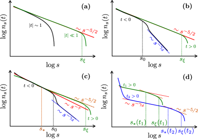
Figure 1: Figure with schematic log-log plots of $n_{s}(t)$ in the various regimes. (a) Homogeneous networks. The red line corresponds to the critical scaling $s^{-\tau}$ with $\tau=5/2$. For $|t|\ll 1$, both positive and negative, an exponential cutoff occurs for for $s=s_{\xi}$ with the correlation scale $s_{\xi}$ diverging as criticality is approached. (b) $\gamma_{d}>4$. The red line corresponds to the critical scaling $s^{-\tau}$ with $\tau=5/2$. For positive $t\ll 1$ (green line), the same picture as in (a) holds. However, for $|t|\ll 1$ but $t<0$ (black line), the asymptotic scaling is given by $s^{-\gamma_{d}}$ (blue dashed line), and the exponent $\tau$ is visible only up to the crossover scale $s_{0}$. (c) $3<\gamma_{d}<4$. The red line corresponds to the critical scaling $s^{-\tau}$ with $\tau=2+1/(\gamma_{d}-2)$. For small positive $t$ (green line), the asymptotic scaling is with an exponent $5/2$ (orange dashed line) followed by an exponential cutoff occurring at $s_{\xi}$, while in the preasymptotic regime $1\ll s\ll s_{*}$ the scaling with exponent $\tau$ is observed. For small $t<0$ (black line) the same picture as in (b) holds. (d) $2<\gamma_{d}<3$. Only the case $t>0$ is possible. The two cases $t_{2}<t_{1}\ll 1$ exhibit the same scaling behavior: a preasymptotic scaling with exponent $\gamma_{d}$, followed (after the scale $s_{*}$) by the exponent $5/2$ and then an exponential cutoff at $s_{\xi}$. However, as $t$ is decreased, the amplitude of these decays decreases and vanishes asymptotically, leaving only $n_{s}(t=0)=\delta_{s,1}$.

On homogeneous networks percolation is perfectly described by the scaling ansatz (23) [see Fig. 1(a)]: the cluster size distribution is a power-law with exponent $\tau=5/2$ cut off exponentially at the correlation size $s_{\xi}$. Both for positive and negative $t$, $s_{\xi}$ diverges as $|t|^{-1/\sigma}$ as criticality is approached, with the mean-field exponent $\sigma=1/2$.

The same scenario applies for power-law networks with $\gamma_{d}>4$ and $t>0$, but for $t<0$ the picture is different [see Fig. 1(b)]: after an exponential cutoff, occurring for $s_{0}\sim|t|^{-1/\sigma}$, the cluster size distribution decays indefinitely as $s^{-\gamma_{d}}$, a legacy of the degree distribution of the original network Newman (2007). This violation of the scaling ansatz Eq. (23) is a direct effect of the heterogeneity of the substrate but it is not related to different critical properties of the percolation process. Indeed, for $t\to 0^{-}$ the asymptotic tail with exponent $\gamma_{d}>\tau$ is not responsible for the divergence of the fluctuations, which are determined instead by the preasymptotic scaling with exponent $\tau$. The scale $s_{0}\sim|t|^{-1/\sigma}$ plays a role similar to the correlation size $s_{\xi}$ for $t>0$ and scales in the same way.

For more heterogeneous networks, $3<\gamma_{d}<4$, both $\sigma$ and $\tau$ become $\gamma_{d}$-dependent, but the most relevant change is that for $t>0$ the asymptotic decay of $n_{s}(t)$ is of the form $s^{-5/2}e^{-s/s_{\xi}}$, i.e., it is different from the decay $s^{-\tau}$ occurring exactly at criticality ($t=0$). The way these two apparently incompatible behaviors are reconciled is depicted in Fig. 1(c): a crossover scale $s_{*}$, smaller than $s_{\xi}$ but diverging with $t$ in the same way, separates the preasymptotic decay $s^{-\tau}$ from the regime $s^{-5/2}e^{-s/s_{\xi}}$. As criticality is approached, both $s_{*}$ and $s_{\xi}$ diverge and the regime $s^{-\tau}$ extends to all scales. For $t<0$ instead the phenomenology is analogous to the case for $\gamma_{d}>4$ only with a different value of $\tau$.

Finally, for $2<\gamma_{d}<3$ only the percolating phase $t>0$ exists, as $\phi_{c}=0$. In contrast to what happens for the other types of networks discussed above, when $\phi\to 0$ the system exhibits no critical behavior: $\langle s\rangle$ does not diverge ($\gamma=-1$), the cluster size distribution tends to be delta distributed ($n_{s}(0)=\delta_{s,1}$), and the correlation length $\xi$ goes to zero ($\nu=-1/2$). However, for small $t$ the cluster size distribution exhibits a nontrivial behavior, displaying some features of a critical transition, see Fig. 1(d). For fixed small $t$, similarly to the case $3<\gamma_{d}<4$, $n_{s}$ exhibits two power-law decays, separated by a crossover scale $s_{*}$. For $1\ll s\ll s_{*}$, it decays as $s^{-\gamma_{d}}$, while for $s\gg s_{*}$ we find $n_{s}\sim s^{-5/2}e^{-s/s_{\xi}}$, where $s_{\xi}\sim t^{-1/\sigma}$, with $\sigma=(3-\gamma_{d})/(\gamma_{d}-2)$. Also the crossover scale $s_{*}$ diverges as $t^{-1/\sigma}$. Hence one could be tempted to conclude that $\tau=\gamma_{d}$, in agreement with some theoretical results in the literature Lee et al. (2004), and in contrast with others Cohen et al. (2002); Li et al. (2021). Note that with this value the scaling relations (29) would not be satisfied. But crucially the large-$s$ tail of $n_{s}$ is multiplied by a $t$-dependent factor, vanishing as $t\to 0$, in agreement with the fact that $n_{s}(\phi)\to\delta_{s,1}$. Despite the fact that $\phi_{c}=0$ is not a veritable critical point it is still possible to write this behavior of $n_{s}(t)$ in a scaling form (23), where now $\tau=2+1/(\gamma_{d}-2)$ (in agreement with Cohen et al. (2002) and with the scaling relations) and the scaling function $f_{+}(x)$ does not go to a constant for $x\to 0$, vanishing instead as $x^{\gamma_{d}-1}$. This nontrivial form of the scaling function $f_{+}(x)$ has the consequence that for fixed $t$ the cluster size distribution decays with an exponent $\gamma_{d}$ different from $\tau$ and a $t$-dependent prefactor vanishing as $t\to 0$.

All these results about $n_{s}(t)$ are in agreement with what one can deduce from the theory for the network component size distribution formulated by Kryven Kryven (2017), adapting the results therein by assuming that nodes are diluted with probability $\phi$ (see Appendix E).

Network type		$\bar{\nu}$	$\theta$	$\frac{1}{\sigma\bar{\nu}}$
Homogeneous		$3$	$\frac{2}{3}$	$\frac{2}{3}$
$4<\gamma_{d}$	$\omega\leq 3(\gamma_{d}-3)$	$3$	$\frac{2}{3}$	$\frac{2}{3}$
	$\omega\geq 3(\gamma_{d}-3)$	$\frac{\omega}{\gamma_{d}-3}$	$1-\frac{\gamma_{d}-3}{\omega}$	$\frac{2(\gamma_{d}-3)}{\omega}$
$3<\gamma_{d}<4$	$\omega\leq\gamma_{d}-1$	$\frac{\gamma_{d}-1}{\gamma_{d}-3}$	$\frac{\gamma_{d}-2}{\gamma_{d}-1}$	$\frac{\gamma_{d}-2}{\gamma_{d}-1}$
	$\omega\geq\gamma_{d}-1$	$\frac{\omega}{\gamma_{d}-3}$	$1-\frac{1}{\omega}$	$\frac{\gamma_{d}-2}{\omega}$
$2<\gamma_{d}<3$		$\frac{\omega}{3-\gamma_{d}}$	$1-\frac{1}{\omega}$	$\frac{\gamma_{d}-2}{\omega}$

Table 2: Values of size-related critical exponents for uncorrelated power-law distributed networks in the various $\gamma_{d}$ ranges, where the hard structural cutoff of the network is taken as $k_{\text{max}}\sim N^{1/\omega}$, with $\omega$ a positive parameter obeying the constraint $\omega\geq 1$ ($\omega\geq 2$ for $2<\gamma_{d}<3$). The homogeneous case corresponds to a sub-algebraically growing $k_{c}(N)$. The hyperscaling relation, Eq. (41), is satisfied when the values in the last two columns coincide (see Appendix C.7).

Also concerning finite-size scaling the picture is surprisingly rich (see Table 2 for a summary of results and Appendix C.7 for a detailed discussion). Contrary to naive expectation and to what is reported in the literature Cohen et al. (2002); Dorogovtsev et al. (2008); Li et al. (2021); Dhara (2018); Dhara et al. (2021), the exponent $\bar{\nu}$, governing how the effective threshold approaches the asymptotic limit, does not necessarily assume the mean-field value $\bar{\nu}=3$ for power-law degree-distributed networks with $\gamma_{d}>4$. Indeed, $\bar{\nu}$ assumes its mean-field value 3 only for small enough $\omega$, the exponent governing how the network hard structural cutoff $k_{\text{max}}$ grows with the system size $N$, $k_{\text{max}}\sim N^{1/\omega}$. Specifically, for $\gamma_{d}>4$ we have $\bar{\nu}=3$ only for $\omega\leq 3(\gamma_{d}-3)$. For $\omega\geq 3(\gamma_{d}-3)$ the exponents $\bar{\nu}$ and $\theta$ depend also on $\omega$ and hyperscaling relations do not hold. The crossover value for $3<\gamma_{d}<4$, above which hyperscaling relations are violated, is $\omega=\gamma_{d}-1$. For $2<\gamma_{d}<3$ the transition occurring at $\phi=0$ is not really critical and the whole finite size scaling framework must be interpreted differently (see Appendix C.7).

V Numerical simulations

We performed numerical simulations to test some of the analytical results, in particular with regard to finite size scaling. We considered networks built according to the uncorrelated configuration model Catanzaro et al. (2005), with $k_{\text{max}}=k_{\text{min}}N^{1/\omega}$, $\omega=3$, $k_{\text{min}}=3$ and various $\gamma_{d}$. Site percolation was simulated by means of the efficient Newman-Ziff algorithm Newman and Ziff (2000) where for each network $M=1000$ realizations were run. To identify the critical point we considered two different susceptibilities Castellano and Pastor-Satorras (2016): $\phi_{c1}$ is the position of the peak of $\chi_{1}=(\langle{\cal S}^{2}\rangle-\langle{\cal S}\rangle^{2})/(\phi N)$, while $\phi_{c2}$ is the position of the peak of $\chi_{2}=(\langle{\cal S}^{2}\rangle-\langle{\cal S}\rangle^{2})/\langle{\cal S}\rangle$. We evaluate the scaling of the size of the largest cluster at criticality for both determinations of the critical point, $S_{1}(N)={\langle\cal S\rangle}|_{\phi_{c1}}(N)/\phi_{c1}(N)\sim N^{\theta}$ and analogously for $S_{2}(N)$. The height of the peak of $\chi_{1}$ scales as $N^{\gamma/{\bar{\nu}}}$ [see Eq. (39)], while the peak of $\chi_{2}$ diverges with an exponent $(\gamma+\beta)/{\bar{\nu}}=1/(\sigma{\bar{\nu}})$. This latter exponent coincides with $\theta$ if hyperscaling holds. We then average all the measured quantities over $100$ to $1000$ different realizations of the network substrate. We finally evaluate the effective exponent $\lambda$ of the observable $O\sim N^{\lambda}$ as a function of size by performing simulations for several sizes $N_{i}$ and calculating

$$\lambda(N_{i})=\frac{\log({O}(N_{i+1})/{O}(N_{i}))}{\log(N_{i+1}/N_{i})}.$$ (81)

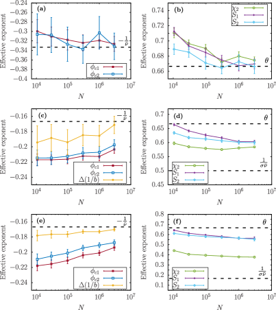
Figure 2: Effective exponents of the observables $\phi_{c1}$, $\phi_{c2}$, $\chi_{2}$, $S_{1}$, and $S_{2}$ measured via Eq. (81) in numerical simulations for power-law networks, with (a),(b) $\gamma_{d}=5$, (c),(d) $\gamma_{d}=3.5$, and (e),(f) $\gamma_{d}=2.5$. Dashed lines correspond to the theoretical predictions of the exponent as in Table 2. Note that in (b), where the hyperscaling is expected to hold, $\theta=1/(\sigma\bar{\nu})$. In (c) and (e), we also report the scaling of the branching factor measured over the network samples, showing the presence of preasymptotic effects.

For $\gamma_{d}=5$, finite size scaling is the same valid for homogeneous networks: $\bar{\nu}=3$, $\theta=2/3$, and hyperscaling holds. Fig. 2(a) confirms that this picture holds for networks with size of the order of $N=10^{6}$ or larger. For $\gamma_{d}=2.5$ instead, we do not expect hyperscaling to hold and the predicted value of $\bar{\nu}$ is 6. While the violation of hyperscaling is clear in Fig. 2(f), it is evident that the effective exponents are far from the predicted asymptotic values. Effective exponents differ from those predicted analytically also for $\gamma_{d}=3.5$ [Fig. 2(d)]. Also in this case strong preasymptotic effects dominate, as shown by Fig. 2(c): while the scaling of $\Delta(1/b)=1/b(N)-1/b_{\infty}$ approaches the expected behavior $N^{-1/6}$ for the largest sizes considered, the effective exponents derived from the scaling of $\phi_{c1}(N)$ and $\phi_{c2}(N)$ are close to $-0.2$. This indicates that the term proportional to $N^{-1/3}$ in Eq. (127) cannot be safely neglected, even for the largest values of $N$ considered. The effective exponent close to $-0.2$ can be interpreted, since $1/{\bar{\nu}}=(\gamma_{d}-3)/\omega$, as the consequence of an effective value of $\omega\approx 2.5$ which, inserted into $\theta=1-1/\omega$, accounts for the effective exponent of $S_{1}$ and $S_{2}$ close to $0.6$. The true asymptotic behavior could be observed only for system sizes such that the blue and red curves in Fig. 2(c),(e) reach the dashed horizontal line. Networks of several orders of magnitude larger than those we can consider would be needed. For the same reason, it is impossible to verify numerically the breakdown of hyperscaling and the validity of the prediction $\bar{\nu}=\omega/(\gamma_{d}-3)$ for $\gamma_{d}>4$ and $\omega\geq 3(\gamma_{d}-3)$.

VI Conclusions

In this paper we have provided a complete and coherent analysis of the critical behavior of standard site and bond percolation models on random uncorrelated networks with generic degree distribution $p_{k}$. This topic has been the subject of intense research activity for decades and a general understanding of many nontrivial features had already been reached a long time ago. In particular the vanishing threshold for strongly heterogeneous networks and the dependence of some critical exponents on the exponent $\gamma_{d}$ have been recognized over 20 years ago Cohen et al. (2000, 2002). However, results about critical properties are scattered in a large body of literature and often interspersed with imprecise or incorrect statements. Moreover a complete theory for all exponents and the scaling functions was lacking. In this work we have filled these gaps. By means of the generating function approach we have derived all critical properties for both infinite and finite systems. In this way we have clarified the true value of some exponents over which confusion existed in the literature, we have derived the value of other exponents not explicity calculated before, and we have determined for the first time critical amplitude ratios.

A crucial finding is the detailed understanding of how the cluster size distribution $n_{s}(t)$ behaves in the various ranges of $\gamma_{d}$ values. It turns out that the usual scaling assumption $n_{s}(t)\sim s^{-\tau}f(s/s_{\xi}(t))$ with $f(x)=\exp(-x^{1/\sigma})$ is never fully correct for power-law distributed networks. For $\gamma_{d}>4$ in the subcritical case the exponential cutoff is followed by an asymptotic decay $s^{-\gamma_{d}}$. For $3<\gamma_{d}<4$ this subcritical feature is accompanied, above the threshold, by a crossover such that the asymptotic decay occurs with an exponent that differs from the critical value $\tau$. For strongly heterogeneous networks ($2<\gamma_{d}<3$) the vanishing threshold implies that $\phi_{c}=0$ is not a true critical point. It is still possible to write $n_{s}(t)$ in a scaling form but $f(x)$ vanishes for $x\to 0$. One of the consequences of this nontrivial scaling is that the decay of $n_{s}(t)$ for fixed $t$ is governed by an exponent $\gamma_{d}$ differing from the Fisher exponent $\tau=2+1/(\gamma_{d}-2)$ and is multiplied by a factor which vanishes as $t\to 0$. The claims in the literature that $\tau$ is equal to $\gamma_{d}$ or not even well defined reflect a partial understanding of the scaling properties, that we have fully elucidated here.

We have also presented a consistent theory for finite-size scaling properties, showing that the exponent $\bar{\nu}$ may depend on how the maximum degree $k_{c}$ diverges with the system size. At odds with all previous literature, we find that this may happen even for $\gamma_{d}>4$, (when all thermodynamic exponents are equal to those for homogeneous systems) provided $k_{c}$ diverges sufficiently slowly. This dependence on the network maximum degree implies that hyperscaling relations, usually assumed to be valid, are violated in this case.

Our work may stimulate further in depth investigation (or reinvestigation) of critical properties for other types of percolation processes on networks. What happens when nodes are removed in a non fully random way, for example targeting first highly Cohen et al. (2001) or poorly Gallos et al. (2005); Caligiuri and Castellano (2020) connected nodes? Or if connected components are defined allowing for gaps in paths connecting nodes (extended-range percolation Cirigliano et al. (2023, 2024))? What can be said about critical exponents and scaling relations when the system undergoes a discontinuous or hybrid transition?

Our results may have implications for epidemic models and spreading processes in general, due to well-established links between such models and percolation theory Pastor-Satorras et al. (2015). Our generating functions approach may also be useful in the analysis of critical properties in other models of interacting systems on networks exhibiting continuous phase transitions, e.g., spin systems, models of synchronization and opinions dynamics Dorogovtsev et al. (2008).

The exploration and understanding of universal behaviors in models defined on complex networks – often qualitatively different from those observed on regular topologies – offer a pathway to deeper theoretical insights into the physics of complex systems, remaining an intriguing challenge for future research.

Appendix A Cluster size distribution of some graph models close to criticality

It is interesting to show the correctness of the scaling ansatz Eq. (23) in cases for which the form of $n_{s}(t)$ can be exactly derived.

A.1 $1$-d chain

For the $1d$ chain $n_{s}(\phi)=\phi^{2}(1-\phi)$ Christensen and Moloney (2005). In this case $\phi_{c}=1$, so that $\phi=1+t$, hence

$$n_{s}(t) =(-t)^{2}(1+t)^{s}=(-t)^{2}\exp(s\ln(1+t))$$

$$=s^{-\tau}f(s^{\sigma}t),$$ (82)

where $s_{\xi}=-1/\ln(1+t)\simeq-t^{-1}$ and $\tau=2$, $\sigma=1$. Note that in this case $f(x)=x^{2}e^{-x}$, hence $f(x)\sim x^{2}$ for $|x|\ll 1$.

A.2 Erdős-Rényi graphs

Unfortunately, there are no other finite dimensional systems for which an exact expression for $n_{s}(t)$ is available. However, in Ref. Newman (2007), Newman brilliantly derived a general formula for the cluster size distribution in random graphs, where he showed that

$$\pi_{s}(\phi)=sn_{s}(\phi)=\frac{\phi^{s-1}\langle k\rangle}{(s-1)!}\left[\frac{d^{s-2}}{dz^{s-2}}\left[g_{1}(z)\right]^{s}\right]_{z=1-\phi}.$$ (83)

For ER graphs with $p_{k}=e^{-c}c^{k}/k!$ this implies

$$\pi_{s}(\phi)=\frac{e^{-cs\phi}(cs\phi)^{s-1}}{s!},$$ (84)

from which it follows, using Stirling’s formula $s!~{}\simeq s^{s}e^{-s}\sqrt{2\pi s}$ for $s\gg 1$, working close to $\phi_{c}=1/c$, hence $c\phi=ct-1$,

$$n_{s}(t) \simeq\frac{s^{-5/2}}{\sqrt{2\pi}}\exp(-s[ct-\ln(1+ct)])$$

$$\simeq\frac{s^{-5/2}}{\sqrt{2\pi}}\exp(-(cs^{1/2}t)^{2}/2])=s^{-\tau}f(cs^{\sigma}t),$$ (85)

which is exactly in the form of Eq. (23), with $f(x)$ Gaussian, and $\tau=5/2$, $\sigma=1/2$.

A.3 Random regular graphs

For random regular networks with degree $c>2$ ($c$-RRN), the generating functions are $g_{0}(z)=z^{c}$ and $g_{1}(z)=z^{c-1}$, hence from Eq. (83)

$$\pi_{s}(\phi) =\phi^{s-1}\langle k\rangle\frac{\Gamma[s(c-1)+1]}{(s-1)!\Gamma[s(c-2)+3]}(1-\phi)^{s(c-2)+2}.$$

Using $\Gamma(x+3)\simeq x^{2}\Gamma(x+1)$, and again Stirling’s formula for $s\gg 1$, we find, after some tedious but straightforward computations,

$$\frac{\Gamma[s(c-1)+1]}{(s-1)!\Gamma[s(c-2)+3]} =s\frac{\Gamma[s(c-1)+1]}{s!\Gamma[s(c-2)+3]}\simeq s[s(c-2)]^{-2}\frac{[s(c-1)]^{s(c-1)}e^{-s(c-1)}\sqrt{2\pi s(c-1)}}{s^{s}e^{-s}\sqrt{2\pi s}[s(c-2)]^{s(c-2)}e^{-s(c-2)}\sqrt{2\pi s(c-2)}}$$

$$=s^{-3/2}\sqrt{\frac{c-1}{2\pi(c-2)}}(c-2)^{-2}\exp\left[s(c-1)\ln(c-1)-s(c-2)\ln(c-2)\right]$$

from which it follows that

$$n_{s}(\phi) \simeq\langle k\rangle\frac{s^{-5/2}}{\phi}\sqrt{\frac{c-1}{2\pi(c-2)}}\left(\frac{1-\phi}{c-2}\right)^{2}\exp\left[-s/s_{\xi}\right],$$

where

$$s_{\xi}^{-1}=-(c-2)\ln\left[\frac{(c-1)(1-\phi)}{(c-2)}\right]-\ln[\phi(c-1)].$$

Since $\phi_{c}=1/(c-1)$, we can write $c-2=(1-\phi_{c})/\phi_{c}$, $(c-1)/(c-2)=1/(1-\phi_{c})$, and $(c-1)(1-\phi)/(c-2)=1-t/(1-\phi_{c})$. Therefore, expanding $\ln(1+x)$ for small $x$ and keeping the lowest orders in $t$

$$s_{\xi}^{-1} \simeq\left(\frac{1}{2\phi_{c}(1-\phi_{c})}+\frac{1}{2\phi_{c}^{2}}\right)t^{2}=\frac{1}{2\phi^{2}_{c}(1-\phi_{c})}t^{2},$$

from which $\sigma=1/2$. For $t\ll 1$, we then have

$$n_{s}(\phi)\simeq\sqrt{\frac{(1+\phi_{c})^{2}}{2\pi(1-\phi_{c})}}s^{-5/2}e^{-s/s_{\xi}},$$ (86)

Hence the scaling ansatz Eq. (23) holds, with a Gaussian scaling function, $\tau=5/2$ and $\sigma=1/2$.

A.3.1 Explicit solution for $c=3$

For $c=3$ it is possible to solve explicitly for $H_{0}(z)$, since the generating functions $G_{0}(z)$ and $G_{1}(z)$ are simple monomials of third and second order, respectively. Indeed, the equation for $H_{1}$,

$$H_{1}=z(\phi H_{1}+1-\phi)^{2},$$

can be explicitly solved

$$H_{1}(z)=\frac{1-2z\phi(1-\phi)-\sqrt{1-4z\phi(1-\phi)}}{2z\phi^{2}},$$

which substituted in the equation

$$H_{0}(z)=z\left(\phi H_{1}(z)+1-\phi\right)^{3},$$

gives

$$H_{0}(z)=\frac{\left[1-\sqrt{1-4z\phi(1-\phi)}\right]^{3}}{8z^{2}\phi^{3}}.$$

The convergence radius of $H_{0}(z)$ is $z^{*}=1/(4\phi(1-\phi))$. Note that its singular behavior close to $z^{*}$ is determined by the singular behavior of $H_{1}(z)$. The singularity is always outsite the unitary circle apart from the critical point $\phi=\phi_{c}=1/2$. Expanding $H_{0}(z)$ close to $z^{*}$, and $z^{*}$ for $\phi$ close to $\phi_{c}$, yields $\tau=5/2$, $\sigma=1/2$.

Appendix B Mean-field theory for percolation and upper critical dimension

A standard procedure in statistical physics to study the critical behavior in finite-dimensional systems is to find an equivalent, coarse-grained, description of the system of interest in terms of a field theory, i.e. a partition function

$$Z=\int\mathcal{D}\varphi e^{-\mathcal{S}[\varphi]}$$ (87)

where $\mathcal{S}[\varphi]$ is

$$\mathcal{S}[\varphi]=\int d^{D}x\left[\frac{1}{2}\varphi\mathop{}\!\mathbin{\bigtriangleup}\varphi+V(\varphi)\right],$$ (88)

$\mathop{}\!\mathbin{\bigtriangleup}$ is the Laplacian operator, and $V(\varphi)$ is in general a function of the ordering field $\varphi$, whose average defines the order parameter. The potential $V$ can be determined on the basis of symmetry considerations, and it strongly depends on the values of the control parameters. If one finds a proper functional form for $\mathcal{S}[\varphi]$, then the study of the critical behavior of the effective field-theory described by Eq. (87) is equivalent to the study of the critical behavior of the finite-dimensional system of interest. For standard percolation, the effective potential contains a cubic term, Aharony (1980); Amit (1976); Cardy (1996)

$$V(\varphi)=\frac{1}{2}c_{2}\varphi^{2}+\frac{1}{3!}c_{3}\varphi^{3}$$ (89)

where $c_{2}\sim\phi-\phi_{c}$ and $c_{3}$ is constant. Since in general it is not possible to solve the integral in Eq. (87), many approximations, perturbative and non-perturbative methods have been developed in the last decades. The starting point remains, however, the so-called Landau approximation. In this zero-th order approximation, one simply neglects spatial fluctuations. This can be physically interpreted as a coarse-graining procedure performed over length scales larger than the correlation length $\xi$. Writing $\varphi(x)=\varphi_{0}+\delta\varphi(x)$, in practice one solves the integral in Eq. (87) ignoring the contributions in $\delta\varphi(x)$. The spatial integral over $d^{D}x$ gives a volume factor, hence one can compute $Z$ using the saddle-point method, which is to find the minimum of $V(\varphi)$, $\varphi_{0}$ such that

$$V^{\prime}(\varphi_{0})=0.$$ (90)

Within this approximation, we can study the critical behavior and compute the critical exponents. However, we must always question whether or not the approximation is justified. We can find the answer in the Ginzburg criterion Goldenfeld (2018), which tells us that for a system whose Landau theory is described by a set of critical exponents $\beta,\gamma,\nu,\dots$, the validity of the description provided by the Landau approximation is conditioned on

$$|t|^{-\gamma-2\beta+D\nu}\ll 1.$$ (91)

Given $D$, this criterion provides an argument to understand whether or not we are “close but not too close” to $t=0$ in order to see the mean-field Landau exponents rather than the $D$-dependent ones. On the other hand, this criterion tells us what is the minimum dimension $D$ of the space above which we are safe in describing our system using the Landau approximation. This dimension is called upper critical dimension and is given by

$$D_{\text{UC}}=\frac{\gamma+2\beta}{\nu}.$$ (92)

In particular, the Landau theory for standard percolation using Eq. (89) gives $\beta=1$, $\gamma=1$, $\nu=1/2$, hence we recover the well-known result $D_{\text{UC}}=6$ Amit (1976). Since Landau theory correctly describes the critical behavior for $D\geq D_{\text{UC}}$, we can conclude that the mean-field Landau theory for percolation, from Eq. (89), is equivalent to percolation on (infinite-dimensional) homogeneous networks. Hence to introduce the idea of space in the infinite-dimensional world of networks we can use standard finite-dimensional results replacing $D$ with $D_{\text{UC}}$.

Homogeneous networks are effectively infinite-dimensional systems and mean-field theory describes well the critical properties of percolation on top of them. However, the effective field theory associated with standard percolation fails to describe the critical behavior of systems with strong heterogeneity in the connectivities and a different theory is necessary Goltsev et al. (2003). In other words, while it is true that percolation on homogeneous networks is equivalent to the mean-field regime of percolation on finite-dimensional systems with $D>6$, percolation on heterogeneous networks obeys the mean-field theory of a different system, in which a singular $\gamma_{d}$-dependent term appears in the effective Hamiltonian Goltsev et al. (2003). In particular, it has been shown Goltsev et al. (2003) that the correct mean-field theory associated to percolation on heterogeneous networks with power-law degree distribution $p_{k}\sim k^{-\gamma_{d}}$ for large $k$ is given by

$$V(\varphi)=\frac{1}{2}c_{2}\varphi^{2}+\frac{1}{3!}c_{3}\varphi^{3}+c_{\gamma_{d}}\varphi^{\gamma_{d}-1}.$$ (93)

We can interpret Eq. (93) as the effective potential of a finite $D$-dimensional system with heterogeneous connectivity of each site. Therefore we can insert the critical exponents of the Landau theory associated to Eq. (93), i.e., the exponents computed in this paper for heterogeneous networks, see Table 1, into the Ginzburg criterion,  (92), to determine the upper critical dimension $D_{\text{UC}}$. Using the values of $\beta$, $\gamma$ and $\nu$ in Table 1, we find

$$D_{\text{UC}}=\begin{cases}6,&\gamma_{d}\geq 4,\\ \frac{2(\gamma_{d}-1)}{(\gamma_{d}-3)},&3<\gamma_{d}<4.\end{cases}$$ (94)

These values are in agreement with previous results in the literature Cohen and Havlin (2004) obtained via different arguments. For $2<\gamma_{d}<3$ Eq. (94) would predict $D_{\text{UC}}<0$. This reflects the fact that in no finite-dimensional space, of any arbitrary large dimension $D$, is the critical behavior described by the Landau theory of Eq. (87) and Eq. (93) equivalent to percolation on heterogeneous networks.

Appendix C Calculations of the critical exponents for random graphs

In this section we develop in detail the computation of all critical exponents for random graphs with homogeneous or power-law degree distributions, following the general recipe described in Sec.III.

For homogeneous degree distributions, such as Erdős-Rényi (ER) or random regular networks, $g_{0}(z)$ and $g_{1}(z)$ are analytic functions, hence they don’t have any singular part. In this case $b=\langle k^{2}\rangle/\langle k\rangle-1$ is the branching factor and $d=\langle k(k-1)(k-2)\rangle/\langle k\rangle$. The case of heterogeneous networks is provided by random graphs with a power-law degree distribution $p_{k}\sim k^{-\gamma_{d}}$, asymptotically for large $k$. In this case it is always possible to write

$$g_{0}(1-x) \simeq 1-\langle k\rangle x+\frac{1}{2}\langle k\rangle bx^{2}+C(\gamma_{d}-1)x^{\gamma_{d}-1},$$ (95)

$$g_{1}(1-x) \simeq 1-bx+\frac{1}{2}dx^{2}+C(\gamma_{d}-2)x^{\gamma_{d}-2},$$ (96)

where $b$, $d$ and $C(\cdot)$ depend on the value of $\gamma_{d}$. For the explicit values of these non-universal coefficients for graphs with $p(k)=(\gamma_{d}-1)k_{\text{min}}^{\gamma_{d}-1}k^{-\gamma_{d}}$, within the continuous degree approximation, see Appendix G in Cirigliano et al. (2023).

C.1 The exponents $\beta$ and $\delta$

C.1.1 Homogeneous degree distributions

From Eqs. (47) and (49) it follows, using $1-b\phi_{c}=0$, that

$$-btm+\frac{1}{2}d\phi^{2}m^{2}\simeq h,$$ (97)

which can be solved for $m$. In particular, at criticality the linear term vanishes and $m\sim h^{1/2}$, hence $\delta=2$ and $E=\phi_{c}\langle k\rangle[2/(\phi_{c}^{2}d)]^{1/2}$. At $h=0$ instead, $m=0$ for $t\leq 0$ and

$$m\simeq\left(\frac{2}{d\phi_{c}^{3}}\right)t,$$ (98)

for $t>0$, hence $1-\Psi(t,0)=2\langle k\rangle t/(d\phi_{c}^{2})$, i.e., $\beta=1$ and $B=2\langle k\rangle/(d\phi_{c}^{2})$.

C.1.2 PL degree distributions

For $\gamma_{d}>4$, $d=\langle k(k-1)(k-2)\rangle$ is finite and the singular part in $g_{1}(1-x)$ does not modify Eq. (97), which is still valid. Hence $\beta=1$, $\delta=2$. In this case, the degree heterogeneity is not strong enough to produce a scenario different from the homogeneous case.

For $3<\gamma_{d}<4$ instead, the singularity $x^{\gamma_{d}-2}$ in $g_{1}(1-x)$ (Eq. (96)) is dominant with respect to the term $x^{2}$ for small $x$. Eq. (47) becomes, using again $1-b\phi_{c}=0$,

$$C(\gamma_{d}-2)\phi^{\gamma_{d}-2}m^{\gamma_{d}-2}-btm=h,$$ (99)

from which it follows that $m\sim h^{1/(\gamma_{d}-2)}$ at criticality, hence $\delta=\gamma_{d}-2$, while $E=\langle k\rangle/[\phi_{c}C(\gamma_{d}-2)]^{1/(\gamma_{d}-2)}$. For $h=0$ instead, $m=0$ for $t\leq 0$, while

$$m\simeq\left[\frac{1}{C(\gamma_{d}-2)\phi_{c}^{\gamma_{d}-1}}\right]^{1/(\gamma_{d}-3)}t^{1/(\gamma_{d}-3)},$$ (100)

for $t>0$, hence $\beta=1/(\gamma_{d}-3)$ and $B=\langle k\rangle[C(\gamma_{d}-2)\phi_{c}^{2}]^{1/(3-\gamma_{d})}$.

The case $2<\gamma_{d}<3$ requires more care. From Eq. (96), the equation for $m$ is, ($t=\phi$ since $\phi_{c}=0$),

$$m(1+|b|t)+C(\gamma_{d}-2)t^{\gamma_{d}-2}m^{\gamma_{d}-2}=h,$$ (101)

where now $b$ is a negative constant and it is no longer the branching factor of the network (which is infinite). Setting $t=0$, we get $m=h$, and from Eq. (50) $\delta=1$. Note that in this case $\Psi(0,h)=e^{-h}\simeq 1-h$ is analytical and no information about the coefficients of its power series for large $s$ can be extracted from its behavior around the origin. Hence formally we have $\delta=1$, $E=1$, but these values are not associated to a singular behaviour, and it is no longer true that $\delta=1/(\tau-2)$, as it will be shown below when $\tau$ is evaluated.

For $h=0$ instead

$$m\simeq\left[-C(\gamma_{d}-2)\right]^{\frac{1}{(3-\gamma_{d})}}t^{(\gamma_{d}-2)/(3-\gamma_{d})},$$ (102)

from which, using Eq. (50) with $\phi=t$, we get $\beta=1+(\gamma_{d}-2)/(3-\gamma_{d})=1/(3-\gamma_{d})$ and $B=\langle k\rangle[-C(\gamma_{d}-2)]^{1/(3-\gamma_{d})}$. For $2<\gamma_{d}<3$ this exponent describes the critical properties of the percolation strength for bond percolation: $\beta_{bond}=\beta$. As explained in the main text, for site percolation the presence of an additional multiplicative factor $\phi$ in the equation for $P^{\infty}$, Eq. (5), implies instead Radicchi and Castellano (2015) $\beta_{\text{site}}=1+\beta_{\text{bond}}=1+1/(3-\gamma_{d})=(4-\gamma_{d})/(3-\gamma_{d})$.

C.2 The exponent $\alpha$

C.2.1 Homogeneous degree distributions

From Eq. (53), expanding $\Psi(\phi,0)$ for small $t$, using $m=m(t,0)$ as in Eq. (98) and $b\phi-1=bt$ we get

$$F(t)\simeq 1-\frac{\langle k\rangle\phi_{c}}{2}-\frac{\langle k\rangle}{2}t+\frac{\langle k\rangle}{2}tm^{2}-\frac{1}{3!}\langle k\rangle d\phi_{c}^{3}m^{3}.$$ (103)

Eq. (103) shows that $F(t)$ approaches a constant value linearly in $t$ as $t\to 0$. However, the exponent $\alpha$ accounts for the behavior of the singular part of $F(t)$, which is given by the terms involving $m$. For homogeneous distributions, since $m\sim t$ for $t>0$ [see Eq. (98)] we get $F(t)\sim t^{3}$, hence $\alpha=-1$, in agreement with the scaling relations. In this case, the exponent governing the behavior of the singular part is, by chance, an integer. As shown below, this is not the case for PL degree distributions.

Note also that, for any $t<0$, $m$ is identically zero. This means that there is no singular contribution in $F(t)$ for $t<0$. Hence the exponent $\alpha$ and the associated amplitude $A_{-}$ are not defined in the nonpercolating phase. For this reason, we did not consider in our analysis two additional amplitude ratios containing $A_{-}$ defined in Aharony (1980).

C.2.2 PL degree distributions

From Eq. (53), expanding $\Psi(\phi,0)$ for small $t$ and using $m=m(t,0)$ we find, neglecting the non-singular term $1-\phi\langle k\rangle/2$,

$$F(t)\simeq\frac{\phi\langle k\rangle}{2}(b\phi-1)m^{2}-\frac{\langle k\rangle d}{3!}\phi^{3}m^{3}+C(\gamma_{d}-1)\phi^{\gamma_{d}-1}m^{\gamma_{d}-1}.$$ (104)

For $\gamma_{d}>4$, the singular term proportional to $m^{\gamma_{d}-1}$ can be neglected. Since $m\sim t$ and $b\phi-1=bt$, as for homogeneous degree distributions we get $\alpha=-1$.

For $3<\gamma_{d}<4$, the only difference is that $m\sim t^{1/(\gamma_{d}-3)}$ [see Eq. (100)], hence at leading singular order

$$F(t)\sim t^{(\gamma_{d}-1)/(\gamma_{d}-3)},$$ (105)

from which $\alpha=(\gamma_{d}-5)/(\gamma_{d}-3)$.

For $2<\gamma_{d}<3$, $\phi=t$, and $m\sim t^{(\gamma_{d}-2)/(3-\gamma_{d})}$ [see Eq. (102)]. Now the leading singular term is the one proportional to $t^{\gamma_{d}-1}m^{\gamma_{d}-1}$ (since $\gamma_{d}-1<2$), so that

$$F(t)\sim t^{(\gamma_{d}-1)/(3-\gamma_{d})},$$ (106)

from which $\alpha=(7-3\gamma_{d})/(3-\gamma_{d})$.

Again the exponent $\alpha$ and the associated amplitude $A_{-}$ are not defined in the nonpercolating phase.

C.3 The exponent $\gamma$

C.3.1 Homogeneous degree distributions

For $t<0$, at $h=0$ we have $m=0$. Hence from Eq. (55)

$$\langle s\rangle-1\simeq\frac{\phi_{c}\langle k\rangle}{-bt}=\phi_{c}^{2}\langle k\rangle|t|^{-1},$$

giving $\gamma=1$ and $C_{-}=\phi_{c}^{2}\langle k\rangle$. As expected, $C_{-}$ is a nonuniversal constant, since it depends on the details of the model. For $t>0$ instead, $m$ is given by Eq. (98), and

$$\langle s\rangle-1\simeq\frac{\phi_{c}\langle k\rangle}{-tb+2bt}=\phi_{c}^{2}\langle k\rangle t^{-1},$$

from which again $\gamma=1$ and the (universal) amplitude ratio is $C_{+}/C_{-}=1$.

C.3.2 PL degree distributions

For $\gamma_{d}>4$, the results obtained for homogeneous distributions hold.

For $3<\gamma_{d}<4$, still $m=0$ for $t<0$, from which we get again the same behavior approaching the threshold from below. For $t>0$ instead, inserting Eq. (100) into Eq. (55) we have at leading order

$$\langle s\rangle-1 \simeq\frac{\phi_{c}\langle k\rangle}{1-\phi\big{[}b-(\gamma_{d}-2)C(\gamma_{d}-2)\phi_{c}^{\gamma_{d}-3}m^{\gamma_{d}-3}\big{]}}$$

$$=\frac{\phi_{c}\langle k\rangle}{-bt+(\gamma_{d}-2)bt}=\frac{\phi_{c}^{2}\langle k\rangle}{(\gamma_{d}-3)}t^{-1}.$$

In this case the exponent is $\gamma=1$ and the critical amplitude ratio is $C_{+}/C_{-}=1/(\gamma_{d}-3)$.

For $2<\gamma_{d}<3$, inserting Eq. (102) into Eq. (55) at leading order we get

$$\langle s\rangle-1 \simeq\frac{t\langle k\rangle}{1-t\big{[}-|b|-(\gamma_{d}-2)C(\gamma_{d}-2)t^{\gamma_{d}-3}m^{\gamma_{d}-3}\big{]}}$$

$$\simeq\frac{\langle k\rangle}{3-\gamma_{d}}t.$$

This implies $\gamma=-1$ and $C_{+}=\langle k\rangle/(3-\gamma_{d})$.

C.4 The exponent $\nu$

C.4.1 Homogeneous degree distributions

Close to criticality, taking $\phi<\phi_{c}$, since $u=1$ and $g_{1}^{\prime}(1)=b$, from Eq. (69) it follows $\xi\simeq(1-\phi b)^{-1/2}=b^{-1/2}(-t)^{-1/2}$. If $t>0$, we have $u=1-m$ and $g_{1}^{\prime}(1-\phi m)$ can be expanded using Eq. (98) obtaining $\xi\simeq(\phi b-1)^{-1/2}=b^{-1/2}t^{-1/2}$. In both cases the prefactor is the same so that the amplitude ratio $\Xi_{+}/\Xi_{-}=1$.

C.4.2 PL degree distributions

For any $\gamma_{d}>3$, since $b$ is finite an analogous argument also applies yielding $\nu=1/2$ and $\Xi_{+}/\Xi_{-}=1$. When $2<\gamma_{d}<3$, instead, since $\phi=t$, the denominator in Eq. (69) goes to a constant, while the numerator is of order $t$. As a consequence, $\xi\sim t^{1/2}$ and hence $\nu=-1/2$.

C.5 The amplitude ratio $R_{\chi}$

C.5.1 Homogeneous degree distributions

Inserting in the definition

$$R_{\chi}=C_{+}E^{-\delta}B^{\delta-1}$$ (107)

the value $\delta=2$ and the expressions for $C_{+}$, $E$ and $B$ derived above for homogeneous distributions yields

$$R_{\chi}=1,$$ (108)

the same universal value obtained on lattices above the upper critical dimension Aharony (1980).

C.5.2 PL degree distributions

For $\gamma_{d}>4$ the amplitudes are the same of the homogeneous case so that $R_{\chi}=1$. For $3<\gamma_{d}<4$ instead, $\delta=\gamma_{d}-2$ and the expressions of the amplitudes $C_{+}$, $B$ and $E$ are different (see Sec. C.1.2). Inserting them into the definition yields $R_{\chi}=1/(\gamma_{d}-3)$, which has the same level of universality of the exponents, i.e., it depends only on $\gamma_{d}$ but not on details of the degree distribution. For $2<\gamma_{d}<3$, since $\delta=1$ and $E=1$ we find $R_{\chi}=C_{+}=\langle k\rangle/(3-\gamma_{d})$. Note that this value is not universal (it depends on $\langle k\rangle$), as it should be. However, we already pointed out that the point $t=0$ for $2<\gamma_{d}<3$ is not a true critical point, and the exponent $\delta=1$, together with the amplitude $E=1$, coming from the analytic part of $\Psi$ are not associated to a critical behavior. However, a nonrigorous argument can be developed to restore criticality and define a universal $R_{\chi}$ even in this case. The argument is as follows. The singular part of $\Psi(t,h)$ can be written, from Eq. (25), as $\{\Psi(t,h)\}_{\text{sing}}=|t|^{\frac{\tau-2}{\sigma}}{\mathcal{F}}_{\pm}^{\prime}(x)$, where ${\mathcal{F}}_{\pm}^{\prime}$ is a scaling function of the variable $x=h/|t|^{1/\sigma}$. The critical behavior – the exponents $\beta$, $\delta$ and the associated critical amplitudes – can be recovered from the cases $x\ll 1$, i.e. $h\to 0$ and $t$ small, and $x\gg 1$, i.e. $t\to 0$ and $h$ small. For $\gamma_{d}>3$ as well as for homogeneous degree distributions, ${\mathcal{F}}_{\pm}^{\prime}(x)\sim 1$ for $x\ll 1$ and ${\mathcal{F}}_{\pm}^{\prime}(x)\sim x^{\tau-2}$ for $x\gg 1$. However, for $2<\gamma_{d}<3$, as no singular part of $\Psi$ remains when $t\to 0$, the scaling behavior of ${\mathcal{F}}_{\pm}^{\prime}(x)$ for $x\gg 1$ must be different, and must correspond to $\{\Psi(t\to 0,h)\}_{\text{sing}}\sim 0$. Working instead at $x=\mathcal{O}(1)$, i.e., small but finite $h$ and $t$, from Eq. (101) it follows, using the value of $\sigma$ in Table 1, at lowest order $m\simeq[-C(\gamma_{d}-2)]^{1/(3-\gamma_{d})}x^{-1}h$. Plugged into Eq. (50), with $\phi=t=x^{-\sigma}h^{\sigma}$, we finally get

$$\Psi(\phi,h)\simeq 1-\langle k\rangle[-C(\gamma_{d}-2)]^{\frac{1}{(3-\gamma_{d})}}x^{\frac{1}{2-\gamma_{d}}}h^{1/(\gamma_{d}-2)},$$

from which $\delta^{\prime}=1/(\gamma_{d}-2)$ and $E^{\prime}=\langle k\rangle[-C(\gamma_{d}-2)]^{\frac{1}{(3-\gamma_{d})}}x^{\frac{1}{2-\gamma_{d}}}$. Using these values, from Eq. (107), we get

$$R_{\chi}=\frac{1}{3-\gamma_{d}}[-C(\gamma_{d}-2)]^{\frac{1}{\gamma_{d}-3}}x.$$

Fixing $x=[-C(\gamma_{d}-2)]^{\frac{1}{3-\gamma_{d}}}$ we then find the universal value $R_{\chi}=1/(3-\gamma_{d})$. Thus for $2<\gamma_{d}<3$ we can formally study the singular behavior of $\Psi$ in the limit $t\to 0$, $h\to 0$ but keeping $x$ fixed as above. Note that $\delta^{\prime}$ is also in agreement with the scaling relation $\tau=2+1/\delta^{\prime}$. The physical motivation for the choice of $x$ remains to be understood.

C.6 The exponents $\sigma$ and $\tau$

C.6.1 Homogeneous degree distributions

Using Eq. (130) and (131) in Appendix D, the solution of the characteristic equation is $\eta=t/(d\phi_{c}^{3})$. Hence, since $u^{*}=1-\eta$

$$\rho=\psi(u^{*})\simeq 1+\frac{1}{d\phi_{c}^{4}}t^{2},$$ (109)

from which, using the definition of $s_{\xi}$ in Eq. (72), $\sigma=1/2$. For $t>0$, $\rho$ is far away from the unitary disk: the presence of the GC strongly hinders the formation of other large clusters, introducing an exponential cutoff Newman (2007). At criticality $\phi=\phi_{c}$, $t=0$, the singularity $\rho$ touches the unitary disk $\rho=1$, and $s_{\xi}$ diverges. For $t<0$, in the phase without a GC, the singularity $\rho$ is again pushed away from the unitary circle since, also in this case, only small clusters can form.

In order to derive $\tau$ we must invert Eq. (78). From the expansion of $\psi(u)$ around $u^{*}$, setting $\epsilon=u^{*}-u$, see Eq. (128), we obtain

$$\rho-z =\psi(u^{*})-\psi(u)\simeq\frac{1}{2}|\psi^{\prime\prime}(u^{*})|\epsilon^{2},$$

which can be inverted to give $\epsilon\sim(\rho-z)^{1/2}$, yielding

$$H_{1}(z)\simeq u^{*}-A_{1}(\rho-z)^{1/2},$$ (110)

with $A_{1}$ a positive constant. This result implies

$$\pi_{s}(\phi)\simeq q_{0}s^{-3/2}e^{-s/s_{\xi}}=q_{0}s^{-3/2}f(q_{1}s^{1/2}t),$$ (111)

from which we find that $\tau=5/2$ and the universal scaling function is Gaussian $f(x)=e^{-x^{2}}$. As noted in Kryven (2017), this behavior is a consequence of the central limit theorem. Note that Eq. (111) holds for any $|t|\ll 1$ (see Fig. 1(a)).

C.6.2 PL degree distributions

For power-law degree-distributed networks it is necessary to analyze separately what happens above and below the threshold and consider various ranges of $\gamma$ values.

$\gamma_{d}>4$

$t>0$:

For positive $t\ll 1$, the expansions of $\psi(u^{*})$ and $\psi^{\prime}(u^{*})$ in Eqs. (132), (133) are equivalent to Eqs. (130),(131), hence we recover again Eq. (109), and $\sigma=1/2$. Furthermore, from Eq. (128) we get for $s\gg 1$

$$n_{s}(t)\sim s^{-5/2}e^{-s/s_{\xi}}.$$ (112)

$t=0$:

At criticality $\psi(u)$ is singular for $u=1$ and its expansion is now given by Eq. (134). However, since $\epsilon^{\gamma_{d}-2}\ll\epsilon^{2}$, we get the same asymptotic behavior as in Eq. (112), even though $\gamma_{d}$-dependent subleading corrections are present. We can conclude that $\tau=5/2$.

$t<0$:

In this case the convergence radius of $H_{1}(z)$ remains $\rho=1$, since the characteristic equation $\psi^{\prime}(u^{*})=0$ admits a solution only for $t>0$. Hence $s_{\xi}=\infty$. In the expansion of $\psi(u)$ around 1 (see Eq. (135)) if the condition

$$-t\ll\epsilon$$ (113)

holds, then the term proportional to $\epsilon$ can be neglected compared to the term $\epsilon^{2}$. In such a case the inversion of Eq. (136) yields

$$\epsilon\simeq(1-z)^{1/2}.$$ (114)

Inserting this into Eq. (113) consistency is found as long as $1-z\gg(-t)^{2}=(-t)^{1/\sigma}$. Hence $n_{s}$ decays with exponent $\tau=5/2$ for $s\ll s_{0}\sim(-t)^{-1/\sigma}$. When this condition is not fulfilled, then at leading order from Eq. (136) $\epsilon\sim(1-z)$ which, replaced back into Eq. (136), gives

$$1-H_{1}(z)=\epsilon=c_{1}(1-z)+\textrm{other reg. terms}+c_{2}(1-z)^{\gamma_{d}-2}.$$ (115)

Since the first term in the r.h.s. is regular, this expression implies, via Eq. (71), that

$$n_{s}(t)\sim s^{-\gamma_{d}}.$$ (116)

In summary, we find the critical decay $n_{s}\sim s^{-5/2}$ for $1\ll s\ll s_{0}$, with $s_{0}\sim|t|^{-1/\sigma}$; for $s\sim s_{0}$, $n_{s}(t)$ exhibits an exponential cutoff and then, for $s\gg s_{0}$, a tail $s^{-\gamma_{d}}$ (see Fig. 1(b)).

Hence, even though the correlation size $s_{\xi}$ is formally infinite for $t<0$, there is another characteristic size $s_{0}$ such that the cluster size distribution can be written as

$$n_{s}(t)\simeq q_{0}s^{-\tau}f_{-}(q_{1}s^{\sigma}t)+q_{2}s^{-\gamma_{d}},$$ (117)

with $f_{-}(x)\ll 1$ for $|x|\ll 1$, showing that the scaling ansatz Eq. (23) must be modified.

Two distinct mechanisms contribute to the cluster size distribution tail in Eq. (117). The first is the collective phenomenon of percolation, where small clusters merge into larger and larger clusters as $t\to 0^{-}$. This mechanism is responsible for the critical properties such as the divergence of $\langle s\rangle$. The second is the presence for any finite $\phi>0$ of a small but finite fraction of nodes with arbitrarily high degree, surrounded by active neighbors, as already noticed in Newman (2007). The contribution of the first mechanism is larger than the second, all the more so when criticality is approached, because $\gamma_{d}>\tau$, so that only the first tail remains as $s_{0}$ diverges. Therefore, even if Eq. (23) is not strictly obeyed, the correction in Eq. (117) can be neglected if we are interested in critical properties.

$3<\gamma_{d}<4$

$t>0$:

For positive $t\ll 1$, in Eq. (133) the subleading term proportional to $\eta$ can be neglected. Inserting the solution of the characteristic equation into Eq. (132) we obtain

$$\rho\simeq 1+\frac{\phi_{c}^{-(\gamma_{d}-2)/(\gamma_{d}-3)}}{\left[(\gamma_{d}-2)C(\gamma_{d}-2)\right]^{1/(\gamma_{d}-3)}}t^{(\gamma_{d}-2)/(\gamma_{d}-3)},$$ (118)

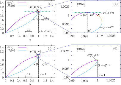
Figure 5: The origin of the crossovers in the cluster size distributions for power-law networks. In this case, $\gamma_{d}=3.5$ is considered. In (a), the functions $\psi(u)$ and its inverse $H_{1}(u)$ are plotted for $t>0$ but $t\ll 1$. In particular, on the scale in (a) it is impossible to detect the difference between $\rho$, $u^{*}$ and $1$, and the system seems to be at criticality $t=0$ and $\rho=1$, with a singular behaviour associated with the critical exponent $\tau$. On a closer look (b), however – hence on a smaller scale – we can distinguish $u^{*}$ from $1$ and a square-root singularity determines the behaviour close to the singularity at $\rho>1$. The asymptotic scaling of $n_{s}$ for large $s\gg s_{*}$ is then determined by the inversion in (b), but for $1\ll s\ll s_{*}$ the picture in (a) is valid and determines the preasymptotic scaling with exponent $\tau$. Similarly, in (c) the situation $t<0$ but $|t|\ll 1$ is considered. At first sight, the system seems to be at criticality $t=0$ in (c), where $\psi^{\prime}(1)=0$. However, on a closer look (d) we realize that $t<0$ since $\psi^{\prime}(1)\neq 0$. Again, the picture in (c) determines the scaling of $n_{s}$ for $1\ll s\ll s_{0}$, while asymptotically we must look closer (d) to find the scaling $n_{s}\sim s^{-\gamma_{d}}$ for $s\gg s_{0}$.

from which $\sigma=(\gamma_{d}-2)/(\gamma_{d}-3)$. Since $t>0$, Eq. (128) can be used again, from which we find again the scaling in Eq. (112). However, now Eq. (128) is valid conditioned on $\epsilon\ll 1-u^{*}=\eta$, because of the presence of the singularity of $G_{1}(u)$ in $u=1$. If we consider the inverse function $H_{1}(z)$ (see Fig. 5) the inversion works only far from the singularity in $z=1$, which implies $\rho-z\ll\rho-1=\psi(u^{*})-1\ll 1$. Hence the asymptotic behavior obtained from Eq. (128) holds provided $s\gg s_{*}$, where

$$s_{*}=\frac{1}{\psi(u^{*})-1}.$$ (119)

In the opposite regime $\psi(u^{*})-1\ll\rho-z\ll 1$, that is for $1\ll s\ll s_{*}$, it is not possible to distinguish $u^{*}$ from $1$, hence $\rho$ from $1$, and the validity of the Taylor expansion breaks down. We can use instead the asymptotic expansion close to $1$ – see Eq. (134) – rather than the Taylor expansion close to $u^{*}$. In this regime, we observe the critical behavior, see the case $t=0$ below. Note that since $s_{\xi}=1/\log(\rho)=1/\log(1+\psi(u^{*})-1)$, and $\log(1+x)\leq x$, we have $s_{*}\leq s_{\xi}$. In particular, $s_{*}\sim s_{\xi}$ for $t\ll 1$.

$t=0$:

In this case Eq. (134) must be used, where now $\epsilon^{2}\ll\epsilon^{\gamma_{d}-2}$. Inverting Eq. (78) implies $\epsilon\sim(\rho-z)^{1/(\gamma_{d}-2)}$ which leads to

$$n_{s}(0)\sim s^{-[2+1/(\gamma_{d}-2)]},$$ (120)

i.e., $\tau=2+1/(\gamma_{d}-2)$.

There is an apparent contradiction: the asymptotic scaling with exponent $5/2$ for any $t>0$ is different from what occurs for $t=0$, where $\tau=2+1/(\gamma_{d}-2)>5/2$. This is at odds with what happens for homogeneous systems (and for $\gamma_{d}>4$) where the value of the exponent is the same and only the cutoff scale $s_{\xi}$ changes as criticality is approached. The conundrum is solved by the presence of the crossover scale $s_{*}$ (discussed above for $t>0$), which separates a decay as $s^{-\tau}$ for $1\ll s\ll s_{*}$ from the asymptotic decay $s^{-5/2}e^{-s/s_{\xi}}$. When $t\to 0$ the crossover size diverges, $s_{*}\sim t^{-1/\sigma}$, while still remaining smaller than the correlation size $s_{*}\leq s_{\xi}$ This does not imply a violation of the scaling ansatz. Eq. (23) is still valid but, analogously to what happens in the case $2<\gamma_{d}<3$ (see below), the scaling function $f_{+}(x)$ has a nonstandard form: it is constant for $x\ll x^{*}=s_{*}/s_{\xi}$; it vanishes exponentially for $x\gg 1$; it behaves as $x^{(4-\gamma_{d})/[2(\gamma_{d}-3)]}$ in the interval between $x^{*}$ and 1.

$t<0$:

The phenomenology is perfectly analogous to the case $\gamma_{d}>4$: $n_{s}(t)$ decays as $s^{-\tau}$ for $1\ll s\ll s_{0}$, where $s_{0}$ diverges as $|t|^{-1/\sigma}$ as criticality is approached. For $s\gg s_{0}$ instead $n_{s}(t)\sim s^{-\gamma_{d}}$. The only difference with respect to the case $\gamma_{d}>4$ is that now $\tau=2+1/(\gamma_{d}-2)$, because the term competing with the linear term in Eq. (135) is $\epsilon^{\gamma_{d}-2}$ instead of $\epsilon^{2}$.

$2<\gamma_{d}<3$

In this range of $\gamma_{d}$ values, only the phase $t>0$ exists and $\phi=t$. We can solve again the characteristic equation using the expansion Eq. (133) for small $\eta$, and from Eq. (132) obtain

$$\rho=1-C(\gamma_{d}-2)[-(\gamma_{d}-2)C(\gamma_{d}-2)]^{1/(3-\gamma_{d})}t^{(\gamma_{d}-2)/(3-\gamma_{d})},$$ (121)

from which $\sigma=(3-\gamma_{d})/(\gamma_{d}-2)$. This result implies the existence of a diverging correlation size $s_{\xi}\sim t^{-1/\sigma}$ even if for $t=0$ no critical behavior occurs.

The asymptotic decay of $n_{s}(t)$ is again determined by the singularity produced by the inversion of $\psi(u)$ close to $u^{*}$

$$H_{1}(z)\simeq u^{*}-c_{1}|\psi^{\prime\prime}(u^{*})|^{-1/2}(\rho-z)^{1/2}.$$ (122)

Hence $n_{s}$ exhibits a tail $s^{-5/2}$ with an exponential cutoff at $s_{\xi}$. As in the case $3<\gamma_{d}<4$, this expression holds provided that $u$ is close enough to $u^{*}$, hence the asymptotic behavior extracted from it holds only for $s\gg s_{*}\sim t^{-1/\sigma}$. For $1\ll s\ll s_{*}$, we can use the expansion in Eq. (129), in perfect analogy to the cases of PL networks for $t<0$ considered above, which gives

$$H_{1}(z)\simeq 1-c_{2}\phi^{\gamma_{d}-2}(1-z)^{\gamma_{d}-2},$$ (123)

corresponding to a power law scaling of $n_{s}$ with exponent $\gamma_{d}$. Following the analogy with the case $3<\gamma_{d}<4$, we may be tempted to identify $\tau=\gamma_{d}$: as $t\to 0$, only the decay with exponent $\gamma_{d}$ survives. However it has to be noted that there are multiplicative factors depending on $\phi$. While they do not play any essential role for $\gamma_{d}>3$, as for $t\ll 1$ they are simply $\phi_{c}>0$ at leading order, the situation now requires a more careful analysis. From Eq. (129), and the expression of $\eta=1-u^{*}$ in terms of $t$, we see that $|\psi^{\prime\prime}(u^{*})|\sim t^{(\gamma_{d}-3)/(\gamma_{d}-2)}=t^{-1/\sigma}$. The concavity of $\psi(u)$ in $u^{*}$ diverges as $t\to 0$. This means that the peak around $u^{*}$ gets not only smaller, but also narrower, as $t\to 0$. This reflects the fact that $\psi(u)=u$ is analytic for $\phi=0$ and there is no peak at all. Hence a prefactor proportional to $t^{1/\sigma}$ multiplies the decay of $n_{s}$ for large $s$. Similarly, the preasymptotic scaling for $1\ll s\ll s_{*}$ contains a prefactor $t^{\gamma_{d}-2}$. Finally, an additional factor $t$ in $n_{s}(t)$ comes from the mapping between the singular behavior of $H_{1}$ and the singular behavior of $H_{0}$, Eq. (70), since $B_{0}=\rho G_{0}^{\prime}(u^{*})A_{1}\sim t$. Putting all these results together

$$n_{s}(t)\simeq\begin{cases}c_{a}t^{\tilde{a}}s^{-\gamma_{d}},&1\ll s\ll s_{*},\\ c_{b}t^{\tilde{b}}s^{-\frac{5}{2}}e^{-s/s_{\xi}},&s\gg s_{*},\end{cases}$$ (124)

where $s_{\xi}\sim s_{*}\sim t^{-1/\sigma}$, $\sigma=(3-\gamma_{d})/(\gamma_{d}-2)$, $\tilde{a}=\gamma_{d}-1$, $\tilde{b}=1/(2\sigma)+1$, and $c_{a},c_{b}$ are constants independent of $t$. The expression in Eq. (124) can be cast in a scaling form like Eq. (23), in which the dependence on $t$ is absorbed in the scaling function. Hence

$$n_{s}(t)\simeq s^{-\tau}f_{+}(q_{1}s^{\sigma}t),$$ (125)

where $\tau=2+1/(\gamma_{d}-2)$ and the scaling function $f_{+}(x)$ behaves now as

$$f_{+}(x)\simeq\begin{cases}(c_{a}/q_{1}^{\tilde{a}})x^{\tilde{a}},&x\ll x_{*},\\ (c_{b}/q_{1}^{\tilde{b}})x^{\tilde{b}}e^{-x^{1/\sigma}},&x\gg x_{*},\end{cases}$$ (126)

with $x_{*}=q_{1}\widetilde{q}$. Note that if $x_{*}>1$, only the first scaling, followed by the exponential cutoff for $x\sim 1$, is observable. This form of the scaling function with $f_{+}(x)\to 0$ as $x\to 0$ is unusual, but note that a similar behavior of the scaling function appears also for the linear chain (see Appendix A), where $n_{s}$ can be put in a scaling form like Eq. (23) with $\tau=2$ and $f_{-}(x)\sim x^{2}\to 0$ for $x\to 0$.

In conclusion, the analysis developed here shows that for $2<\gamma_{d}<3$ the cluster size distribution obeys the scaling form in Eq. (23) with $\sigma=(3-\gamma_{d})/(\gamma_{d}-2)$, $\tau=2+1/(\gamma_{d}-2)$ but with a scaling function $f_{+}(x)\sim x^{\gamma_{d}-1}$ for $x\to 0$. This implies that if the decay of $n_{s}(t)$ with $s$ is studied at fixed $t$ (as it is usually the case) the exponent measured is not $\tau$ but $\gamma_{d}$ with a prefactor decreasing as $t\to 0$.

C.7 The exponent $\bar{\nu}$

For power-law degree-distributed networks with $\gamma_{d}>3$, $b(k_{c})\simeq b_{\infty}-C_{2}k_{c}^{-(\gamma_{d}-3)}$, where $b_{\infty}=b(k_{c}=\infty)$ and $C_{2}$ is a positive constant. Inserting this expression into Eq. (80) we obtain, at lowest order,

$$\phi_{c}(N,k_{c})\simeq b_{\infty}^{-1}+\frac{C_{2}}{b_{\infty}^{2}}k_{c}^{-(\gamma_{d}-3)}+b_{\infty}^{-1}C_{1}N^{-1/3}.$$ (127)

If degrees are sampled from a distribution with a hard (structural) cutoff $k_{\text{max}}(N)\sim N^{1/\omega}$ the actual cutoff in a realization of the network is the minimum between the structural cutoff and the natural one, $N^{1/(\gamma_{d}-1)}$. This implies that in full generality $k_{c}(N)\sim N^{1/{\tilde{\omega}}}$ with ${\tilde{\omega}}=\max[\omega,\gamma_{d}-1]$ .

Then, considering Eq. (127), the scaling of the effective threshold depends on whether $(\gamma_{d}-3)/{\tilde{\omega}}$ is larger or smaller than $1/3$.

For ${\tilde{\omega}}\leq 3(\gamma_{d}-3)$ the second to last term in Eq. (127) decays faster than the last one; as a consequence $\bar{\nu}=3$ as in the fully homogeneous case: the scaling of the effective threshold $\phi_{c}(N)$ is governed by bona fide critical fluctuations. This occurs for $\gamma_{d}\geq 4$ and $\omega\leq 3(\gamma_{d}-3)$.

If instead ${\tilde{\omega}}\geq 3(\gamma_{d}-3)$ the role of the two contributions is reversed: in this case, for asymptotically large $N$ the second to last contribution in Eq. (127) dictates the scaling of $\phi_{c}(N)$, yielding ${\bar{\nu}}={\tilde{\omega}}/(\gamma_{d}-3)$. For $3<\gamma_{d}<4$ and $\omega\leq\gamma_{d}-1$ (so that ${\tilde{\omega}}=\gamma_{d}-1$) this implies ${\bar{\nu}}=(\gamma_{d}-1)/(\gamma_{d}-3)$. Otherwise ${\tilde{\omega}}=\omega$ and ${\bar{\nu}}=\omega/(\gamma_{d}-3)$, see Fig. 3. The fact that $\bar{\nu}$ depends on the parameter $\omega$, which governs how the thermodynamic limit is reached, immediately implies that the hyperscaling relation (41) is violated as the left hand side cannot depend on $\omega$. The violation of (41) can be traced back to the breakdown of Eq. (40). In its turn this is interpreted as follows: the slow growth of the maximum degree $k_{c}$ with $N$ introduces an additional cutoff smaller than $s_{\xi}$ in the cluster size distribution.

For $2<\gamma_{d}<3$ the picture is completely different. The argument based on the mapping to an appropriate field-theory puzzlingly yields a negative upper critical dimension. It is more useful to observe that the negative value of the exponent $\nu=-1/2$ indicates that the correlation length does not diverge for $\phi\to\phi_{c}=0$. The threshold $\phi_{c}=0$ is not a true critical point. If one insists on determining numerically the behavior of the correlation length $\xi$ as a function of $\phi$, one finds a peak in a position $\phi_{c}(N)\approx b(k_{c}(N))^{-1}$ but with an amplitude that decreases with the system size ($\gamma=-1$). In principle it is possible to define in this way an exponent $\bar{\nu}=\omega/(3-\gamma_{d})$, but with this value hyperscaling relation  (41) is violated.

The rich finite size scaling phenomenology just described is summarized in Fig. 3.

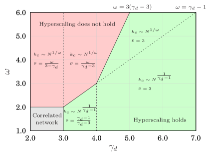
Figure 3: Finite size scaling behavior as a function of $\gamma_{d}$ and $\omega$.

The exponent $\theta$ is readily obtained from Eq. (38). In the region where hyperscaling holds $\theta=2/3$ for $\gamma_{d}>4$ and $\theta=(\gamma_{d}-2)/(\gamma_{d}-1)$ for $3<\gamma_{d}<4$. These values coincide with those obtained using Eq. (40). Instead, when hyperscaling is violated, we find: $\theta=1-(\gamma_{d}-3)/\omega$ for $\gamma_{d}>4$; $\theta=1-1/\omega$ for $\gamma_{d}<4$. These values do not coincide with those obtained from Eq. (40): $1/(\sigma{\bar{\nu}})=2(\gamma_{d}-3)/\omega$ for $\gamma_{d}>4$; $1/(\sigma{\bar{\nu}})=(\gamma_{d}-2)/\omega$ for $\gamma_{d}<4$. Table 2 presents all these results as a function of $\omega$ for the different ranges of $\gamma_{d}$.

Appendix D Asymptotic expansions of $\psi(u)$ and $\psi^{\prime}(u)$

In this Appendix we write the asymptotic expansions of $\psi(u^{*})$ and $\psi^{\prime}(u^{*})$ [see Eq.(73)] for $u^{*}$ close to 1 and also the expansion of $\psi^{\prime}(u)$ for $u$ close to $u^{*}$. We remind that $\psi(u)=u/G_{1}(u)$, where $G_{1}(u)=g_{1}(\phi u+1-\phi)$ and that $u^{*}$ is the solution of the characteristic equation $\psi^{\prime}(u^{*})=0$. These expansions are needed in Appendix C to determine the form of the cluster size distribution $n_{s}(\phi)$. Indeed, in order to determine $\sigma$ we need $s_{\xi}$ for $|t|\ll 1$, which can be evaluated, via Eq. (72), using the expression of $\rho=\psi(u^{*})$. The condition $|t|\ll 1$ implies $u^{*}=1-\eta(t)$ with $\eta\ll 1$. Moreover, to evaluate $\tau$ we must invert Eq. (78) to find $\epsilon=u^{*}-u$ as a function of $\rho-z$ and hence the exponent $a_{1}=a_{0}$, to be inserted in Eq. (71). In some cases this inversion process is far from trivial and is characterized by crossovers between competing behaviors, giving rise to preasymptotic effects in the shape of $n_{s}(\phi)$, see Fig. 1. The main formulas we are going to use are the Taylor expansion of $\psi(u)$ close to $u^{*}$, setting $\epsilon=u^{*}-u$,

$$\psi(u)\simeq\psi(u^{*})-\frac{1}{2}|\psi^{\prime\prime}(u^{*})|^{2}\epsilon^{2},$$ (128)

where we assume $|\psi^{\prime\prime}(u^{*})|\neq 0$, and the asymptotic expansion for $u$ close to $1$, setting $\varepsilon=1-u$,

$$\psi(u)\simeq 1-(1-\phi b)\varepsilon-\frac{1}{2}d\phi^{2}\varepsilon^{2}-C(\gamma_{d}-2)\phi^{\gamma_{d}-2}\varepsilon^{\gamma_{d}-2}.$$ (129)

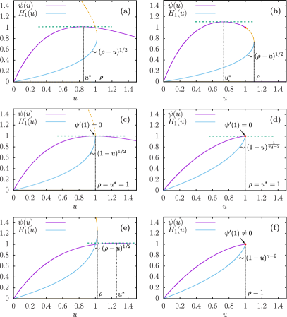
Figure 4: Various plots of the functions $\psi(u)$ (purple) and its inversion $H_{1}(u)$ (blue). The yellow dashed line is the non-physical part produced by the inversion of $\psi(u)$. In the different rows the cases $t>0$, $t=0$ and $t<0$, respectively, are considered. In the left column results are for homogeneous networks, in particular ER graphs, in the right column for power-law network with $\gamma=3.5$. The asymptotic scaling of $H_{1}$ for $\rho-u\ll 1$ is reported. Dashed lines serve as guide to the eye to indicate when the derivative of $\psi(u)$ vanishes (green dashed), in $u^{*}$ (black dotted), and the corresponding convergence radius $\rho$ of $H_{1}$ (black dashed). The red dot signals the presence of a singularity at $u=1$ in $\psi(u)$, but not necessarily in $H_{1}$, see panel (b). While for homogeneous networks the inversion always produces a square-root singularity, i.e. for $t>0$ (a), $t=0$ (c), $t<0$ (e), for power-law networks the inversion produces three different exponents in (b), (d), and (f) corresponding to different scaling asymptotes for $n_{s}(t)$. Note that the exponents in (d) and (f) look similar, but they are different, as explained in detail in Fig. 5.

D.1 Homogeneous degree distributions

For homogeneous distributions $G_{1}(z)$ is analytic and both $\psi(u^{*})$ and $\psi^{\prime}(u^{*})$ can be Taylor expanded [see Fig. 4]. In practice this amounts to use Eq. (129) without the singular term on the r.h.s.. Evaluating it in $u^{*}=1-\eta(t)$, that is $\varepsilon=\eta(t)$, we have for $|t|\ll 1$, $\eta\ll 1$, keeping only the lowest orders in $\eta$

$$\psi(u^{*}) \simeq 1+bt\eta,$$ (130)

$$\psi^{\prime}(u^{*}) \simeq-bt+d\phi_{c}^{2}\eta.$$ (131)

The behavior of $\psi(u)$ for $u$ close to $u^{*}$, setting $\epsilon=u^{*}-u$, is instead given by Eq. (128). Note that these expansions are valid for any $t$, both positive and negative.

D.2 Power-law degree distributions

For power-law degree distributions more care must be taken. The main problem is that $\psi(u)$ is no longer analytic in $u=1$, because of the singularity of $G_{1}(u)$ in $u=1$. Let us discuss separately the three cases $t>0$, $t=0$, and $t<0$. In the first case, $u^{*}<1$ and $\psi(u)$ can still be Taylor expanded around $u^{*}$, using Eq. (128). However, as it will be shown, the validity of such expansion breaks down as $t$ gets small. For $t\leq 0$ instead, the singular behavior of $G_{1}(u)$ around $1$ must be considered and hence Eq. (129) must be used.

D.2.1 Expansions for $t>0$

In this case, setting $u^{*}=1-\eta(t)$ we can write, at lowest order in $\eta$, using Eq. (129)

$$\psi(u^{*}) \simeq 1-(1-\phi b)\eta-C(\gamma_{d}-2)\phi^{\gamma_{d}-2}\eta^{\gamma_{d}-2},$$ (132)

$$\psi^{\prime}(u^{*}) \simeq(1-\phi b)+d\phi^{2}\eta+(\gamma_{d}-2)C(\gamma_{d}-2)\phi^{\gamma_{d}-2}\eta^{\gamma_{d}-3}.$$ (133)

Note that these expansions are defined only for $\eta>0$, hence for $t>0$, in contrast to the case of homogeneous degree distributions, where $\eta<0$ for $t<0$.

Expanding $\psi(u)$ for $u$ close to $u^{*}$ we get again Eq. (128) since, provided that $u^{*}<1$, we can Taylor expand $G_{1}(u)$ in a neighborhood of $u^{*}$.

However, Eq. (128) is valid conditioned on $\epsilon\ll 1-u^{*}=\eta$, because of the presence of the singularity of $G_{1}(u)$ in $u=1$ (see Fig. 4(b)). As shown in Appendix C, this feature leads to preasymptotic effects in the behavior of $n_{s}(t)$.

D.2.2 Expansions for $t=0$

At criticality $u^{*}=1$ and the local behavior of $\psi(u)$ for $u$ close to $u^{*}$ now strongly depends on the value of $\gamma_{d}$. We can no longer Taylor expand $\psi(u)$ (see Fig. 4(d)) and the asymptotic expansion in Eq. (129) must be used instead, obtaining

$$\psi(u)\simeq 1-\frac{1}{2}d\phi^{2}\epsilon^{2}-C(\gamma_{d}-2)\phi^{\gamma_{d}-2}\epsilon^{\gamma_{d}-2},$$ (134)

where $d=\langle k(k-1)(k-2)\rangle/\langle k\rangle>0$ for $\gamma_{d}>4$, while $d$ is a negative constant for $\gamma_{d}<4$ when $\langle k^{3}\rangle=\infty$. As explicitly discussed in Appendix C, the value of the exponent $\tau$ depends on which of the two terms depending on $\epsilon$ in Eq. (134) is the leading order.

D.2.3 Expansion for $t<0$

In this case, the maximum of $\psi(u)$ is now reached in $u^{*}=1$, not because the first derivative vanishes but because $\psi(u)$ is defined only for $u\leq 1$ (see Fig. 4(f)). Hence, setting $1-b\phi=-bt$,

$$\psi(u)\simeq 1+bt\epsilon-\frac{1}{2}d\phi^{2}\epsilon^{2}-C(\gamma_{d}-2)\phi^{\gamma_{d}-2}\epsilon^{\gamma_{d}-2},$$ (135)

that can be rewritten as

$$1-z\simeq-bt\epsilon+\frac{1}{2}d\phi^{2}\epsilon^{2}+C(\gamma_{d}-2)\phi^{\gamma_{d}-2}\epsilon^{\gamma_{d}-2}.$$ (136)

The effect of the competition between the different contributions in these expressions on the behavior of $n_{s}(t)$ is nontrivial, as reported in Appendix C

Appendix E Connection with Kryven’s results

In Ref. Kryven (2017) Kryven presented a general theory to determine the size distribution of connected components in an infinite network built according to the configuration model and specified by an arbitrary degree distribution. The expressions presented there can be used to determine asymptotic properties of the cluster size distribution for a percolation process on the same network by considering that, under dilution, the tail of the degree distribution remains a power-law with the same exponent. In particular, if $q_{k}=Ak^{-(\gamma_{d}-1)}$ is the excess degree distribution of the network with $\phi=1$, after the dilution $q_{k}(\phi)\sim A_{\phi}k^{-(\gamma_{d}-1)}$ for large $k$, where $A_{\phi}=A\phi^{\gamma_{d}-2}$. In other words, dilution affects the small $k$ part of the degree distribution, while the tail remains with the same exponent, only with a different prefactor. All the nontrivial behaviors derived by means of the generating function approach and in particular in Fig. 1, can be worked out from the expressions in Table II in Kryven (2017). In particular, it is interesting to see this connection for the case $2<\gamma_{d}<3$. From Table II in Kryven (2017) and the preasymptotic scaling of the cluster size distribution (see the unnumbered equation below Table II) we find, using the crucial observations that $s_{\text{Kryven}}\sim t^{\gamma_{d}-2}$ and $\mu_{1,{\text{Kryven}}}=t\langle k\rangle$,

$$\pi_{s}(t)\sim\begin{cases}q_{a}t^{\tilde{a}}s^{-(\gamma_{d}-1)},&1\ll s\ll s_{*},\\ q_{b}t^{\tilde{b}}s^{-\frac{3}{2}}e^{-s/s_{\xi}},&s\gg s_{*},\end{cases}$$ (137)

where $s_{\xi}\sim t^{-1/\sigma}$, $\sigma=(3-\gamma_{d})/(\gamma_{d}-2)$, $\tilde{a}=\gamma_{d}-1$, $\tilde{b}=1/(2\sigma)+1$, and $q_{a},q_{b}$ are constants independent of $t$. This is in perfect agreement with Eq. (124). Similar arguments can be developed for $\gamma_{d}>3$, recovering the rich picture of crossover phenomena described here.

References

- Stauffer and Aharony (2018) D. Stauffer and A. Aharony, Introduction to Percolation Theory (CRC press, 2018).
- Machta (1991) J. Machta, “Phase transitions in fractal porous media,” Phys. Rev. Lett. 66, 169 (1991).
- Moon and Girvin (1995) K. Moon and S. M. Girvin, “Critical behavior of superfluid 4 He in aerogel,” Phys. Rev. Lett. 75, 1328 (1995).
- Sahimi (1994) Muhammad Sahimi, Applications of percolation theory (CRC Press, 1994).
- Grassberger (1983) P. Grassberger, “On the critical behavior of the general epidemic process and dynamical percolation,” Math. Biosci. 63, 157 (1983).
- Cardy and Grassberger (1985) J L Cardy and P Grassberger, “Epidemic models and percolation,” Journal of Physics A: Mathematical and General 18, L267 (1985).
- Newman (2002) M. E. J. Newman, “Spread of epidemic disease on networks,” Phys. Rev. E 66, 016128 (2002).
- Cohen et al. (2000) Reuven Cohen, Keren Erez, Daniel ben Avraham, and Shlomo Havlin, “Resilience of the internet to random breakdowns,” Phys. Rev. Lett. 85, 4626–4628 (2000).
- Callaway et al. (2000) D. S. Callaway, M. E. J. Newman, S. H. Strogatz, and D. J. Watts, “Network robustness and fragility: Percolation on random graphs,” Phys. Rev. Lett. 85, 5468–5471 (2000).
- Holme et al. (2002) P. Holme, B. J. Kim, C. N. Yoon, and S. K. Han, “Attack vulnerability of complex networks,” Phys. Rev. E 65, 056109 (2002).
- Goldenfeld (2018) N. Goldenfeld, Lectures on phase transitions and the renormalization group (CRC Press, 2018).
- Patashinsky and Pokrovsky (1979) A. Z. Patashinsky and V. N. Pokrovsky, Fluctuation Theory of Phase Transitions (Pergamon Press, 1979).
- Christensen and Moloney (2005) K. Christensen and N. R. Moloney, Complexity and Criticality, Vol. 1 (World Scientific Publishing Company, 2005).
- Aharony (1980) A. Aharony, “Universal critical amplitude ratios for percolation,” Phys. Rev. B 22, 400–414 (1980).
- Karrer et al. (2014) Brian Karrer, M. E. J. Newman, and Lenka Zdeborová, “Percolation on sparse networks,” Phys. Rev. Lett. 113, 208702 (2014).
- Hamilton and Pryadko (2014) Kathleen E. Hamilton and Leonid P. Pryadko, “Tight lower bound for percolation threshold on an infinite graph,” Phys. Rev. Lett. 113, 208701 (2014).
- Goltsev et al. (2008) A. V. Goltsev, S. N. Dorogovtsev, and J. F. F. Mendes, “Percolation on correlated networks,” Phys. Rev. E 78, 051105 (2008).
- Cantwell and Newman (2019) G. T. Cantwell and M. E. J. Newman, “Message passing on networks with loops,” Proc. Natl. Acad. Sci. USA 116, 23398–23403 (2019).
- Cohen et al. (2002) R. Cohen, D. Ben-Avraham, and S. Havlin, “Percolation critical exponents in scale-free networks,” Phys. Rev. E 66, 036113 (2002).
- Dorogovtsev et al. (2008) S. N. Dorogovtsev, A. V. Goltsev, and J. F. F. Mendes, “Critical phenomena in complex networks,” Rev. Mod. Phys. 80, 1275–1335 (2008).
- Li et al. (2021) Ming Li, Run-Ran Liu, Linyuan Lü, Mao-Bin Hu, Shuqi Xu, and Yi-Cheng Zhang, “Percolation on complex networks: Theory and application,” Physics Reports 907, 1–68 (2021), percolation on complex networks: Theory and application.
- Lee et al. (2004) D.-S. Lee, K.-I. Goh, B. Kahng, and D. Kim, “Evolution of scale-free random graphs: Potts model formulation,” Nuclear Physics B 696, 351–380 (2004).
- Radicchi and Castellano (2015) F. Radicchi and C. Castellano, “Breaking of the site-bond percolation universality in networks,” Nat. Commun. 6, 10196 (2015).
- Newman (2007) M. E. J. Newman, “Component sizes in networks with arbitrary degree distributions,” Phys. Rev. E 76, 045101 (2007).
- Kryven (2017) I. Kryven, “General expression for the component size distribution in infinite configuration networks,” Phys. Rev. E 95, 052303 (2017).
- Newman et al. (2001) M. E. J. Newman, S. H. Strogatz, and D. J. Watts, “Random graphs with arbitrary degree distributions and their applications,” Phys. Rev. E 64, 026118 (2001).
- Newman (2010) Mark Newman, Networks (Oxford university press, 2010).
- Flajolet and Sedgewick (2009) P. Flajolet and R. Sedgewick, Analytic Combinatorics (Cambridge University Press, Cambridge, 2009).
- Wattendorff and Wessel (2024) Jonas Wattendorff and Stefan Wessel, “Sublattice-selective percolation on bipartite planar lattices,” Phys. Rev. E 109, 044108 (2024).
- Dorogovtsev and Mendes (2022) S. N. Dorogovtsev and J. F. F. Mendes, The Nature of Complex Networks (Oxford University Press, 2022).
- Lee et al. (2016a) D. Lee, S. Choi, M. Stippinger, J. Kertész, and B. Kahng, “Hybrid phase transition into an absorbing state: Percolation and avalanches,” Phys. Rev. E 93, 042109 (2016a).
- Lee et al. (2016b) D. Lee, M. Jo, and B. Kahng, “Critical behavior of k-core percolation: Numerical studies,” Phys. Rev. E 94, 062307 (2016b).
- Dhara (2018) Souvik Dhara, “Critical percolation on random networks with prescribed degrees,” (2018), arXiv:1809.03634 [math.PR] .
- Dhara et al. (2021) Souvik Dhara, Remco van der Hofstad, and Johan S. H. van Leeuwaarden, “Critical percolation on scale-free random graphs: New universality class for the configuration model,” Communications in Mathematical Physics 382, 123–171 (2021).
- Catanzaro et al. (2005) Michele Catanzaro, Marián Boguñá, and Romualdo Pastor-Satorras, “Generation of uncorrelated random scale-free networks,” Phys. Rev. E 71, 027103 (2005).
- Newman and Ziff (2000) M. E. J. Newman and R. M. Ziff, “Efficient monte carlo algorithm and high-precision results for percolation,” Phys. Rev. Lett. 85, 4104–4107 (2000).
- Castellano and Pastor-Satorras (2016) Claudio Castellano and Romualdo Pastor-Satorras, “On the numerical study of percolation and epidemic critical properties in networks,” The European Physical Journal B 89, 243 (2016).
- Cohen et al. (2001) Reuven Cohen, Keren Erez, Daniel ben Avraham, and Shlomo Havlin, “Breakdown of the internet under intentional attack,” Phys. Rev. Lett. 86, 3682–3685 (2001).
- Gallos et al. (2005) Lazaros K. Gallos, Reuven Cohen, Panos Argyrakis, Armin Bunde, and Shlomo Havlin, “Stability and topology of scale-free networks under attack and defense strategies,” Phys. Rev. Lett. 94, 188701 (2005).
- Caligiuri and Castellano (2020) Annalisa Caligiuri and Claudio Castellano, “Degree-ordered-percolation on uncorrelated networks,” Journal of Statistical Mechanics: Theory and Experiment 2020, 113401 (2020).
- Cirigliano et al. (2023) L. Cirigliano, C. Castellano, and G. Timár, “Extended-range percolation in complex networks,” Phys. Rev. E 108, 044304 (2023).
- Cirigliano et al. (2024) Lorenzo Cirigliano, Claudio Castellano, and Ginestra Bianconi, “General theory for extended-range percolation on simple and multiplex networks,” arXiv preprint arXiv:2407.04585 (2024), https://doi.org/10.48550/arXiv.2407.04585.
- Pastor-Satorras et al. (2015) Romualdo Pastor-Satorras, Claudio Castellano, Piet Van Mieghem, and Alessandro Vespignani, “Epidemic processes in complex networks,” Rev. Mod. Phys. 87, 925 (2015).
- Amit (1976) Daniel J Amit, “Renormalization of the potts model,” Journal of Physics A: Mathematical and General 9, 1441 (1976).
- Cardy (1996) John Cardy, Scaling and renormalization in statistical physics, Vol. 5 (Cambridge University Press, 1996) pp. 145–168.
- Goltsev et al. (2003) A. V. Goltsev, S. N. Dorogovtsev, and J. F. F. Mendes, “Critical phenomena in networks,” Phys. Rev. E 67, 026123 (2003).
- Cohen and Havlin (2004) Reuven Cohen and Shlomo Havlin, “Fractal dimensions of percolating networks,” Physica A: Statistical Mechanics and its Applications 336, 6–13 (2004), proceedings of the XVIII Max Born Symposium ”Statistical Physics outside Physics”.