Eigenvector Localization and Universal Regime Transitions in Multiplex Networks: A Perturbative Approach

Abstract

In this work, we investigate the transition between layer-localized and delocalized regimes in a general contact-based social contagion model on multiplex networks. We begin by analyzing the layer-localization to delocalization transition through the inverse participation ratio (IPR). Utilizing perturbation analysis, we derive a new analytical approximation for the transition point and an expression for the IPR in the non-dominant layer within the localized regime. Additionally, we examine the transition from a non-dominant to a dominant regime, providing an analytical expression for the transition point. These transitions are further explored and validated through dynamical simulations.

I Introduction

Since the inception of multiplex network theory Cozzo et al. (2018); Kivelä et al. (2014), a central focus has been to determine how critical behaviors in these networks differ from those observed in traditional monoplex networks. A key aspect of this exploration involves relating these critical behaviors to the spectral properties of the supra-adjacency matrices and the supra-LaplaciansSánchez-García et al. (2014). One of the critical phenomena intrinsically related to multiplexity is layer-localization, where certain dynamics or structural features become confined to specific layers of the network. The layer-localized/delocalized transition of the endemic steady state in a Susceptible-Infected-Susceptible (SIS) dynamics on multiplex networks was initially described in de Arruda et al. (2017). This phenomenon pertains to the spectral properties of the supra-adjacency matrix, which serves as the dynamical operator describing the process on a multiplex network. Restricting ourselves to a two-layer system, the eigenvalue problem for the supra-adjacency matrix reads:

$$\left[\begin{array}[]{c|c}A_{1}&pI\\ \hline\cr pI&A_{2}\\ \end{array}\right]\cdot\left[\begin{array}[]{c}v_{1}\\ \hline\cr v_{2}\\ \end{array}\right]=\lambda\cdot\left[\begin{array}[]{c}v_{1}\\ \hline\cr v_{2}\\ \end{array}\right]$$ (1)

The fact that nodal infection probabilities at the steady state can be expressed as a linear combination of the eigenvectors of the dynamical operatorGoltsev et al. (2012); de Arruda et al. (2017) allows the study of the layer-localization/delocalization transition in terms of these eigenvectors. Specifically, depending on the inter-layer coupling parameter $p$, the leading eigenvector may become localized in one layer, the dominant one, i.e., the one with the largest leading eigenvalueCozzo et al. (2013), or delocalized across all layers. This property is commonly quantified using the Inverse Participation Ratio (IPR) of the leading eigenvector:

$$IPR(\mathbf{v})=\sum_{i=1}^{N}v_{i}^{4},$$ (2)

where $N$ is the number of nodes-layer pairs in the multiplex network. The summation in 2 can be broken into $m$ parts, where $m$ is the number of layers. For the case of two layers, $IPR(v)=IPR(v_{1})+IPR(v_{2})=IPR_{1}+IPR_{2}$. Additionally, from a dynamical perspective, the modified susceptibility, which measures fluctuations in the system, exhibits a double peak in the localized regime, with only one peak diverging, and a single diverging peak in the delocalized regimede Arruda et al. (2017). More recently, in Ferraz de Arruda et al. (2020), the authors numerically showed that the IPR curves collapse onto a universal curve when the coupling parameter is properly rescaled, where the scaling factor is linearly related to the mean degree difference between layers. For a two-layer multiplex network, they numerically found that the scaling parameter follows the equation $p^{*}\approx\beta_{1}<k_{1}-k_{2}>+\beta_{2}$, where $k_{\alpha}$ is the mean degree of layer $\alpha$, independently of the details of the system. $p^{*}$ separates the layer-localized regime from the delocalized one, and the IPR curves collapse when plotted against $p/p^{*}$. In Ferraz de Arruda et al. (2020), $p^{*}$ is defined as the value of the coupling parameter $p$ at which the power-law trend of the $IPR_{2}$ that characterizes the localized regime and its constant trend that characterizes the delocalized regime intersect. In analogy with the fictive temperature defined in glassy systemsMauro et al. (2009), we call this the fictive coupling.

In this work, we generalize these results to contact-based contagious processes on multiplex networks and demonstrate how the fictive coupling $p^{*}$ can be derived analytically through a perturbative analysis of the leading eigenvector of the supra-contact probability matrix. Furthermore, we establish a connection between this phenomenon and another phenomenon investigated in Cozzo et al. (2013), namely, the switching of the dominant layer based on the intra-layer activity.

II Supra contact probability matrix

Let us now define the main mathematical object of our analysis.The contact probability matrix $\mathbf{R(A)}=\{R(A)_{ij}\}$ was introduced in Gómez et al. (2010) in the context of a contact-based Markov chain approach to epidemic spreading in single layer networks. Its elements are given by

$$R(A)_{ij}=1-\left(1-\frac{A_{ij}}{k_{i}}\right)^{\gamma_{i}},$$ (3)

with $A_{ij}$ the elements of the adjacency matrix $\mathbf{A}=\{A_{ij}\}$, and $k_{i}$ the degree of the node $i$. The element $R(A)_{ij}$ is the probability of node $i$ contacting node $j$ and depends on the activity parameter $1\leq\gamma_{i}$. When $\gamma_{i}=\gamma=1$, $R(A)_{ij}=\frac{A_{ij}}{k_{i}}$ and it describes a contact process, conversely, when $\gamma\to\infty$, $R(A)_{ij}\to A_{ij}$, and the fully reactive process is recovered. In Cozzo et al. (2013), the contact probability matrix is generalize to a multiplex network. In this scenario we have $R_{\alpha}=R(A_{\alpha})$ for each layer. Thus, the supra-contact probability matrix is given by

$$\bar{R}=\bigoplus_{\alpha}R_{\alpha}+pC,$$ (4)

where the first part is the direct sum of each layer contact probability matrix and C is a matrix where $C_{ij}=1$ if the same node is present on different layers. Therefore, the supra-contact probability matrix has a block structure with $R_{\alpha}$ on the diagonal and the $p*C$ out of this diagonal, for instance $\bar{R}=\left(\begin{array}[]{c|c}R_{1}&C_{12}\\ \hline\cr C_{21}&R_{2}\\ \end{array}\right)$ for a two layer multiplex network. Furthermore, when considering the discrete time evolution equation for the contagion probability of a node $i$ Cozzo et al. (2013), we got

$$\vec{p}(t+1)= [\vec{1}-\vec{p}(t)]*[\vec{1}-\vec{q}(t)]+(1+\mu)*\vec{p}(t)$$ (5)

$$+\mu*[\vec{1}-\vec{q}(t)]*\vec{p}(t),$$

where $q_{i}(t)=\prod_{j}[1-\beta R_{ij}p_{j}(t)]$ is the probability to not be infected for the node-layer pair $i$, with $p=\frac{\epsilon}{\beta}$, where $\beta$ characterizes the contagion rate within layers and $\epsilon$ characterizes the contagion rate between the same node in different layers.$\mu$ being the probability of an active state decaying to an inactive one. The phase transition to an endemic phase is given by$\left(\frac{\beta}{\mu}\right)_{c}=\frac{1}{\Lambda_{max}}$ Cozzo et al. (2013), where $\Lambda_{max}$is the largest eigenvalue of the supra-contact probability matrix (4).

III Perturbative analysis

In this section, we study the localization properties of the leading eigenvector of the supra-contact probability matrix through a perturbative analysis of the IPR to obtain the characteristic value of the localized-delocalized regime transition, i.e. the fictive coupling $p^{*}$. We first consider random regular networks (RRNs) due to the simplicity of the calculations. Later, we will show that these results are generalizable to other networks models.

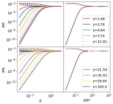
Figure 1: The top panels are a representation of the inverse participation ratio as a function of $p$ and $p/p^{*}$. It is a regular network with $k_{1}=10$, $k_{2}=8$ and 100 nodes. The bottom panels are also a representation of $IPR$ as a function of $p$ and $p/p^{*}$. It is a Erdös-Rényi network with $\langle k_{1}\rangle=10$, $\langle k_{2}\rangle=8$ and 1000 nodes.

Let us consider the case where $p\ll 1$. In the supra-contact probability matrix $\bar{R}=\bigoplus_{\alpha}R_{\alpha}+pC$, the p-dependent part can be treated as a perturbation. Therefore, we can approximate the leading eigenvalue $\bar{\Lambda}\approx\Lambda_{0}+p\Delta\Lambda$ and the corresponding leading eigenvector $\vec{v}\approx\vec{v}_{0}+p\Delta\vec{v}$, where $\Lambda_{0}$ and $\vec{v}_{0}$ are the leading eigenvalue and eigenvector of the uncoupled system. For the uncoupled system, $R=\bigoplus_{\alpha}R_{\alpha}$ is a diagonal block matrix, its eigenvalues are those of the $R_{\alpha}$, thus $\Lambda_{0}$ is the leading eigenvalue of the dominant layer and $\vec{v}_{0}=\left[\begin{array}[]{c}v_{0}\\ \hline\cr 0\\ \end{array}\right]$ is its associated eigenvector, with $v_{0}$ the leading eigenvector of the dominant layer. Considering RRNs, the largest eigenvalue of each layer is $\Lambda_{\alpha}=k_{\alpha}\cdot(1-(1-\frac{1}{k_{\alpha}})^{\gamma_{\alpha}})$ and its corresponding eigenvector is a normalized vector of all ones. The first-order approximation is given by (assuming normalized eigenvectors)

$$\Delta\Lambda_{max}=\vec{v}^{\top}_{0}C\vec{v}_{0}$$ (6)

$$\Delta\vec{v}=\sum_{u_{0}\not=v_{0}}\frac{\vec{u}^{\top}_{0}C\vec{v}_{0}}{\Lambda_{v_{0}}-\Lambda_{u_{0}}}\vec{u}_{0},$$ (7)

where $\vec{u}_{0}$ are the non-leading eigenvectors. Since the leading eigenvectors of two RRNs are equal, the non-leading eigenvector of one of the layer are orthogonal also to the leading eigenvector of the other, there is just one term in the sum in (7) that is not equalto zero. Therefore, $\Delta\Lambda=0$ and $\Delta\vec{v}=\frac{p}{\Lambda_{1}-\Lambda_{2}}C\vec{v}_{0}$. Consequently, the resulting vector is

$$\vec{v}=\left(\begin{array}[]{c}\vec{v}_{0}\\ \hline\cr\frac{p}{\Lambda_{1}-\Lambda_{2}}\vec{v}_{0}\\ \end{array}\right).$$ (8)

Now, we can obtain $p^{*}$ as the $p$ at which $IPR_{1}\approx IPR_{2}$, therefore, $p^{*}=\Lambda_{1}-\Lambda_{2}$

$$p^{*}=k_{1}\left(1-\left(1-\frac{1}{k_{1}}\right)^{\gamma_{1}}\right)-k_{2}\left(1-\left(1-\frac{1}{k_{2}}\right)^{\gamma_{2}}\right).$$ (9)

It results that when $p$ is scaled with $p*$, the IPR curves for different $\gamma$ values collapse onto a universal curve, as shown in Fig. 1. These results have been obtained assuming that we have a RRN in each layer. However, the summation of the products between non-dominant layer non-leading eigenvector and the leading eigenvector of the dominant layer equals zero on average for other network models as well, leading to the same result (see Fig. 1 bottom panel).

Considering the $IPR_{2}$ for $p<p^{*}$, from the perurbative results we have

$$IPR_{2}\approx\left(\frac{p}{\Lambda_{1}-\Lambda_{2}}\right)^{4}$$ (10)

The numerical result given in Ferraz de Arruda et al. (2020) is $\log{IPR_{2}}=\alpha\log(p)+c_{1}$. They obtained that $\alpha\approx 4$ and $c_{1}$ was dependant of the network, and it coincides with our analytical result $\alpha=4$ and $c_{1}\approx-4\log(\Lambda_{1}-\Lambda_{2})$.

IV Non-dominant to dominant transition

It is interesting to study how IPR behaves when changing $\gamma$ for one of the layers. As $\gamma$ grows, the leading eigenvalue associated to the layer till eventually cross the value of the dominant layer and becoming dominant Cozzo et al. (2013).

Let us consider a system of two RRNs with the first layer with $\gamma_{1}\xrightarrow{}\infty$ and $k_{1}=10$ and the second with $k_{2}=30$ and a variable $\gamma$. In this scenario, for low values of $\gamma$, the dominant layer is the first as it has the larger eigenvalue. Then, when surpassing $\gamma*$ (the point where $\Lambda_{1}=\Lambda_{2}$), there is a dominance change where the second layer has the largest eigenvalue. As we know the expression for the eigenvalue in a RRN, we can calculate the analytical expression of $\gamma*$

$$\gamma*=\frac{\ln{\left(1-\frac{\Lambda_{1}}{k_{2}}\right)}}{\ln{\left(1-\frac{1}{k_{2}}\right)}}$$ (11)

Using the numbers of the example, $\gamma*=11.96$ where $\Lambda_{1}=k_{1}$. This result is exact for a RR network. For an Erdös-Rényi network, we can approximate $\gamma*$ using $\Lambda\approx<k>+1$. In the previous example, $\gamma*\approx 13.47$ for an ER network with $\Lambda_{1}\approx<k_{1}>+1$.

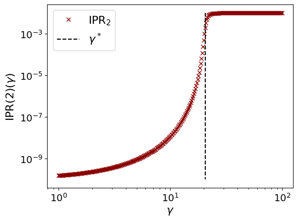
Figure 2: Representation of $IPR_{2}$ as a function of $\gamma$ for a fixed $p=0.1$. Layer 1 has a fixed value of $\gamma\xrightarrow{}\infty$. Its a regular network with 100 nodes and $k_{1}=10$ and $k_{2}=12$. In this network, $\gamma^{*}=20.59$

The change of dominance is showed in Fig. 2, where the IPR for the second layer for low values of $\gamma$ has the non-dominant form and, then, when $\gamma^{*}$ is surpassed, it behaves as the dominant layer.

V Dynamical behaviour at the regimes transitions

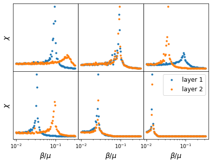
Figure 3: The top panels are $\chi$ in function of $\beta/\mu$ with $\eta=0.1$, the layer 1 with $k_{1}=10$, $\Lambda_{1}\approx 11$ with $\gamma_{1}\xrightarrow{}\infty$ and the layer 2 with $k_{2}=30$, $\Lambda_{2}\approx 31$ and $\gamma_{2}$ variable. Left to right, (i) first layer dominance regime with $\gamma_{2}=5$, (ii) near the dominance change with $\gamma_{2}=13.5$, (iii) second layer dominance regime with $\gamma_{2}$ = 100. The transition point is $\gamma^{*}=13.47$. The bottom panels are $\chi$ in function of $\beta/\mu$ for different values of $\eta$. The layer 1 with $k_{1}=30$, $\Lambda_{1}\approx 31$ and $\gamma_{1}=\infty$. The layer 2 with $k2=10$, $\Lambda_{2}\approx 11$ and $\gamma_{2}=10000$. Left to right, (i4) localized regime with $\eta=0.01$, (i5) near the localization transition with $\eta=15$, (i6) delocalized regime with $\eta=50$. The fictive coupling is $p*=20$.

We perform Monte Carlo simulations on an ER two-layer multiplex network, utilizing a quasi-stationary algorithm de Oliveira and Dickman (2004) to simulate the contagion process. Our focus is on examining the dynamical behavior associated with the regime transitions discussed earlier: the layer-localized to delocalized transition and the dominance transition. These transitions can be characterized using the modified susceptibility, defined as

$$\chi=N\frac{\langle\rho\rangle^{2}-\langle\rho^{2}\rangle}{\langle\rho\rangle},$$ (12)

where $\rho$ is the density when the stationary state is reached and $N=nM$The susceptibility as a function of the structural parameter exhibits a diverging peak at the point of transition, with the peak position being inversely related to the largest eigenvalue of the system. Importantly, since we are concerned only with the peak positions, the normalization factor is not of interest. In a multiplex network, we can analyze the density of each layer individually. In this context, each layer’s susceptibility shows a peak at its transition point; however, only the peak corresponding to the dominant layer will diverge.

We conducted simulations by varying network structural parameters to study the transitions analyzed in previous sections. To investigate the localized-delocalized transition, we varied $\eta=\frac{\epsilon}{\beta}$ which corresponds to the coupling parameter $p$ in the IPR study. For the dominant-to-non-dominant transition, we varied $\gamma_{2}$ for the second layer.

In Fig. 3, we illustrate different structural configurations that are informative for studying these regimes. The top panels focus on the dominance transition. When $\gamma_{2}^{*}>\gamma_{2}$ , layer one dominates, with a diverging peak at $\frac{\beta}{\mu}=\frac{1}{\Lambda_{1}}$ , while layer two shows its peak at $\frac{\beta}{\mu}=\frac{1}{\Lambda_{2}}$. As $\gamma_{2}$ increases, $\Lambda_{2}$ also increases, causing the peak to shift. When $\Lambda_{1}=\Lambda_{2}$, both layers exhibit a diverging peak at the same position and when $\Lambda_{1}<\Lambda_{2}$ the second layer’s peak diverges at $\frac{\beta^{*}}{\mu}=\frac{1}{\Lambda_{2}}$. The bottom panels focus on the localized to delocalized transition. Layer one consistently shows a diverging peak at $\frac{\beta}{\mu}=\frac{1}{\Lambda_{1}}$. . For low values of $\eta$ the second layer exhibits a peak at $\frac{\beta}{\mu}=\frac{1}{\Lambda_{2}}$, however, as $\eta$ increases, this secondary peak disappears and reappears at the position of the layer one peak. When $\eta\gg\eta^{*}$, layers one and two behave similarly, both showing a diverging peak.

VI Conclusions

In this work, we have deduced a first order perturbation approximation for the fictive coupling that characterizes the localised to delocalized transition for a social-contagion model on multiplex networks, $p^{*}$. With this approximation we also have obtained an analytical form for the non-dominant $IPR_{i}$ when $p<p^{*}$, coinciding with the numerical results in Ref. Ferraz de Arruda et al. (2020).

Furthermore, we have studied a dominance transition when varying $\gamma$ for one layer, mentioned before in Ref. Cozzo et al. (2013). We have given an analytical expression for the transition point, $\gamma^{*}$.

Our results completely characterize these regime transitions, giving a direct understanding of the mechanism causing it. However, the real nature of the layer-localized/delocalized transition is still elusive. In fact, structural transitions in multiplex networks are usually related to an eigenvalues crossing De Arruda et al. (2018); Gomez et al. (2013), while in this setting it seams not to be the case.