A Single-Loop Finite-Time Convergent Policy Optimization Algorithm for Mean Field Games (and Average-Reward Markov Decision Processes)

Abstract

We study the problem of finding an equilibrium of a mean field game (MFG) – a policy performing optimally in a Markov decision process (MDP) determined by the induced mean field, where the mean field is a distribution over a population of agents and a function of the policy itself. Prior solutions to MFGs are built upon either the contraction assumption on a mean field optimality-consistency operator or strict weak monotonicity. The class of problems satisfying these assumptions represent only a small subset of MFGs, to which any MFG admitting more than one equilibrium does not belong. In this work, we expand the class of solvable MFGs by introducing a “herding condition” and propose a direct gradient-based policy optimization algorithm that provably finds an (not necessarily unique) equilibrium within the class. The algorithm, named Accelerated Single-loop Actor Critic Algorithm for Mean Field Games (ASAC-MFG), is data-driven, single-loop, and single-sample-path. We characterize the finite-time and finite-sample convergence of ASAC-MFG to a mean field equilibrium building on a novel multi-time-scale analysis. We support the theoretical results with illustrative numerical simulations.

As an additional contribution, we show how the developed novel analysis can benefit the literature on average-reward MDPs. An MFG reduces to a standard MDP when the transition kernel and reward are independent of the mean field. As a byproduct of our analysis for MFGs, we get an actor-critic algorithm for finding the optimal policy in average-reward MDPs, with a convergence guarantee matching the state-of-the-art. The prior bound is derived under the assumption that the Bellman operator is contractive, which never holds in average-reward MDPs. Our analysis removes this assumption.

Keywords— Mean field games, average-reward Markov decision process, actor-critic algorithms

1 Introduction

The mean field game (MFG) framework, introduced in Huang et al. (2006); Lasry and Lions (2007), provides an infinite-population approximation to the $N$-agent Markov game with a large number of homogeneous agents. It addresses the increasing difficulty in solving Markov games as $N$ scales up and finds practical applications in many domains including resource allocation (Li et al., 2020; Mao et al., 2022), wireless communication (Xu et al., 2018; Narasimha et al., 2019; Jiang et al., 2019), and the management of power grids (Alasseur et al., 2020; Zhang et al., 2021b).

A mean field equilibrium describes the notion of solution in an MFG, and is a pair of policy and mean field such that the policy performs optimally in a Markov decision process (MDP) determined by the mean field and the mean field is the induced stationary distribution of the states when every agent in the infinite population adopts the policy. In the discrete-time setting without explicit knowledge of the environment dynamics, reinforcement learning (RL) is an important framework for finding a mean field equilibrium using samples of the state transition and reward. A series of recent works have proposed finite-time convergent RL solutions to MFGs, which either make an assumption on the contraction of a mean field optimality-consistency operator (Guo et al., 2019; Xie et al., 2021; Anahtarci et al., 2023; Mao et al., 2022; Zaman et al., 2023; Yardim et al., 2023) or assume that the MFG is strictly weakly monotone (Perrin et al., 2020; Perolat et al., 2021; Geist et al., 2021; Zhang et al., 2024). However, as pointed out in Yardim et al. (2024), the former assumption only holds if an impractically large regularization is added. Since the policy at the regularized equilibrium quickly approaches a uniform distribution as the regularization weight increases, solving such a regularized problem is usually uninformative about the original game. The latter assumption is also restrictive, reflected by the fact that strictly weakly monotone MFGs may only have one unique equilibrium whereas multiple equilibria usually exist in practical problems (Nutz et al., 2020; Dianetti et al., 2024). The aim of this paper is to expand our knowledge on the class of solvable MFGs and to design a convenient-to-implement, provably convergent, and efficient algorithm for solving MFGs. We summarize our main contributions below and include a literature comparison in Table 1.

Main Contributions
$\bullet\,\,$ We propose a single-loop, single-sample-path policy optimization algorithm ASAC-MFG for finding the equilibrium in an infinite-horizon average-reward MFG, without imposing the aforementioned assumptions. However, it is shown in Yardim et al. (2024) that solving general MFGs (even with Lipschitz transition kernel and reward function) is a PPAD-complete problem conjectured to be computationally intractable (Daskalakis et al., 2009). We identify a subclass of MFGs satisfying a proposed “herding condition” (Assumption 4), which contains instances not observing either the contraction assumption or strict weak monotonicity and can be optimally solved by ASAC-MFG. In this sense, our work complements and expands on the finding of Yardim et al. (2024) and enlarges the class of solvable MFGs. (See Figure. 2)

$\bullet\,\,$ We explicitly characterize the finite-time and finite-sample complexity of ASAC-MFG. On MFGs satisfying the herding condition with $\Delta=0$, ASAC-MFG converges to a global mean field equilibrium with a rate of $\widetilde{{\cal O}}(k^{-1/4})$; for $\Delta>0$, it converges to a $\sqrt{\Delta}-$approximate MFE with the same rate. As our algorithm draws exactly one sample in each iteration, the finite-time complexity translates to an finite-sample complexity of the same order. To our knowledge, this work is the first to study a finite-time convergent algorithm for MFGs without the contraction/monotonicity assumption, and is also the first to propose a completely sample-based single-loop single-sample-path algorithm for MFGs with finite-time guarantees. The single-loop and single-sample-path structure make our algorithm much easier and more convenient to implement than those in the existing literature. Single-loop single-sample-path RL algorithms are widely used in practice due to simplicity but their theoretical understanding is not as complete as their nested-loop counterparts. Our work fills in this important gap in the context of MFGs.

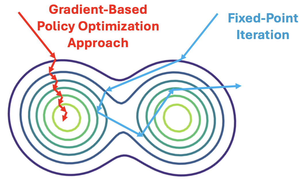
Figure 1: Possible trajectories of gradient-based versus fixed-point iteration methods in the landscape of MFG cumulative return without the contraction assumption. Fixed-point iteration may diverge on the unregularized problem, while gradient-based method converges.

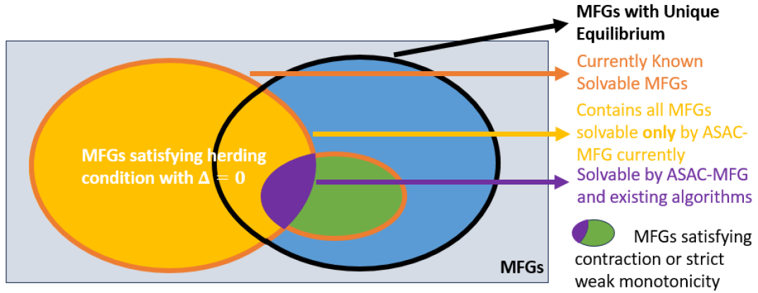
Figure 2: Herding Condition & Subclasses of Mean Field Games.

$\bullet\,\,$ We extend the techniques of analyzing two-time-scale actor-critic algorithms (Wu et al., 2020; Chen and Zhao, 2024) to the three-time-scale case where the additional time scale is introduced to carry out the mean field updates. Our proof is based on a novel multi-time-scale analysis. The additional time scale may prevent the selection of the most suitable step sizes and result in convergence rate degradation if not treated properly. We overcome the challenge by incorporating the latest innovation in convergence acceleration through smoothed gradient estimators (Zeng and Doan, 2024). Our multi-time-scale algorithm design methodology and analysis can be of independent interest and potentially applicable to other problems where the goal is to solve a coupled system of optimization problems.

$\bullet\,\,$ We can regard a Markov decision process (MDP) as a degenerate MFG in which the transition kernel and reward are independent of the mean field. Recognizing this connection, in Sec.5, we note that a simplified version of the proposed method becomes an actor-critic algorithm in an average-reward MDP and is guaranteed to converge to a stationary point of the policy optimization objective with rate $\widetilde{{\cal O}}(1/\sqrt{k})$. This matches the state-of-the-art analysis of the actor-critic algorithm (Chen and Zhao, 2024). However, in this prior work an unrealistic assumption is made on the Bellman back operator that can be shown to never hold. We establish our convergence rate without making this assumption, making our algorithm practical and reliable.

1.1 Related Work

The classic works on MFGs study the continuous-time setting where the equilibrium point simultaneously satisfies a Hamilton–Jacobi–Bellman equation on the optimality of the policy and a Fokker–Planck equation that describes the dynamics of the mean field, and have proposed optimal control techniques that provably find the solution (Huang et al., 2006, 2007; Lasry and Lions, 2007). In discrete time, MFGs can be considered a generalization of MDPs and are widely solved using RL. Among the latest representative works, Yang et al. (2018); Carmona et al. (2021); Perolat et al. (2021) build upon policy optimization and Anahtarcı et al. (2020); Angiuli et al. (2022, 2023); Gu et al. (2023); An et al. (2024) consider valued-based methods. The algorithms proposed in these works, however, either do not come with convergence analysis or are only shown to converge asymptotically.

Finite-time convergent algorithms have been developed under the contraction assumption or strict weak monotonicity. Both assumptions imply the uniqueness of the mean field equilibrium, whereas multiple equilibria usually exist in practical applications (Nutz et al., 2020; Dianetti et al., 2024), violating the assumptions. Leveraging the contraction assumption or by enforcing the assumption through an entropy regularization, Guo et al. (2019); Xie et al. (2021); Anahtarci et al. (2023); Mao et al. (2022); Zaman et al. (2023); Yardim et al. (2023) design fixed-point-iteration-type algorithms, whose sample complexities we detail in Table 1. Perrin et al. (2020); Geist et al. (2021); Zhang et al. (2024) study solving strictly weakly monotone MFGs with mirror descent or fictitious play. The algorithm proposed in Zhang et al. (2024) has a complexity matching that of ASAC-MFG, but is less convenient to implement due to its nested-loop structure and the requirement to pre-generate and store offline samples. Perrin et al. (2020) proposes a continuous-time algorithm and Geist et al. (2021) studies a deterministic gradient algorithm not based on samples, so their complexities are not directly comparable. Without the contraction/monotonicity assumption, algorithms designed in the existing works, especially those based on fixed-point iteration, lose convergence/stability guarantees and may in theory exhibit arbitrary behaviors even when close to an equilibrium, as illustrated in Figure. 1. In contrast, even when a MFG does not satisfy the herding condition with $\Delta=0$, there always exists a positive $\Delta$ for which the herding condition holds, and our algorithm is guaranteed to be stable in the sense that it roughly converges to a region around an equilibrium with radius $\sqrt{\Delta}$.

It is worth pointing out the relevant works (Carmona et al., 2019; Fu et al., 2020; Zaman et al., 2020; Wang, 2024; Zaman et al., 2024) on linear-quadrtic MFGs (i.e. the state and action are continuous, the cost is a quadratic function of state and action, and the state transition is linear), which can be regarded as an extension of the single-agent linear-quadratic regulator. The linear-quadratic structure makes this class of problems more convenient to study and efficient to solve.

Finally, we note the separate line of works (Guo et al., 2024; Mandal et al., 2023) that reformulate the MFG policy optimization problem as a constrained program with convex constraints and a bounded objective. The simple projected gradient descent algorithm provably solves the constrained program, leading to a solution of the MFG. However, a finite-time convergence guarantee is not established, unless again a sufficiently large regularization is added.

	Assumption	Single Sample Path	Single Loop	Sample Complexity
Guo et al. (2019)	Contraction	No	No	Regularization Dependent
Anahtarcı et al. (2020)	Contraction	No	No	-
Xie et al. (2021)	Contraction	Yes*	Yes*	$\widetilde{{\cal O}}(\epsilon^{-5})^{\dagger}$, regularized solution
Mao et al. (2022)	Contraction	No	No	$\widetilde{{\cal O}}(\epsilon^{-5})^{\dagger}$, regularized solution
Zaman et al. (2023)	Contraction	Yes	No	$\widetilde{{\cal O}}(\epsilon^{-4})^{\dagger}$, regularized solution
Yardim et al. (2023)	Contraction	Yes	No	$\widetilde{{\cal O}}(\epsilon^{-2})^{\dagger}$, regularized solution
Zhang et al. (2024)	Monotonicity	No	No	$\widetilde{{\cal O}}(\epsilon^{-4})$, original solution
Our Work	MFG subclass $\Delta=0$	Yes	Yes	$\widetilde{{\cal O}}(\epsilon^{-4})$, original solution
Our Work	Other MFG instances	Yes	Yes	$\widetilde{{\cal O}}(\epsilon^{-4})$, $\sqrt{\Delta}$-optimal solution

Table 1: Existing algorithms and their assumption, structure, and complexity. * The algorithm in Xie et al. (2021) is single-loop and single-sample-path under an oracle that returns the stationary distribution of states for any $\pi,\mu$. Mao et al. (2022) also relies on such an oracle. Our work, in comparison, is oracle-free. ^† If these works could choose the regularization weight freely (note that they actually cannot since the contraction operator assumption only holds when the weight is sufficiently large), they can solve the original unregularized game by making the weight small enough. The complexities, however, at least double, i.e. become $\widetilde{{\cal O}}(\epsilon^{-10})$, $\widetilde{{\cal O}}(\epsilon^{-8})$, $\widetilde{{\cal O}}(\epsilon^{-4})$ to the original solution.

The rest of the paper is organized as follows. Sec.2 presents the MFG formulation. Sec.3 develops the proposed ASAC-MFG algorithm. In Sec.4 we introduce the technical assumptions and state our main theoretical results. Sec.5 discusses an application of our main theorem to policy optimization in average-reward MDPs. Simulation results are presented in Sec.6. Due to the space limit, we defer the literature survey to Appendix 1.1.

2 Formulation

We study MFGs in the stationary infinite-horizon average-reward setting, in which we denote the finite state and action spaces by ${\cal S}$ and ${\cal A}$. From the perspective of a single representative agent, the state transition depends not only on its own action but also on the aggregate behavior of all other agents. Mathematically, we describe this aggregate behavior by the mean field $\mu\in\Delta_{{\cal S}}$, which conceptually measures the percentage of population in each state. The transition kernel of an MFG is represented by ${\cal P}:{\cal S}\times{\cal A}\times\Delta_{{\cal S}}\rightarrow\Delta_{{\cal S}}$, where ${\cal P}(s^{\prime}\mid s,a,\mu)$ describes the probability that the state of the representative agent transitions from $s$ to $s^{\prime}$ when it takes action $a$ and mean field is $\mu$. The mean field also affects the reward function $r:{\cal S}\times{\cal A}\times\Delta_{{\cal S}}\rightarrow[0,1]$ – the agent receives reward $r(s,a,\mu)$ when it takes action $a$ in state $s$ under mean field $\mu$. Not directly observing the mean field, the agent takes actions according to policy $\pi:{\cal S}\rightarrow{\cal A}$, which is represented as $\Delta_{{\cal A}}^{{\cal S}}\subset\mathbb{R}^{|{\cal S}|\times|{\cal A}|}$.

Under a given policy $\pi$ and mean field $\mu$, the states sequentially generated form a Markov chain with transition matrix $P^{\pi,\,\mu}\in\mathbb{R}^{|{\cal S}|\times|{\cal S}|}$, where $P^{\pi,\,\mu}_{s^{\prime},s}=\textstyle\sum_{a\in{\cal A}}{\cal P}(s^{\prime}\mid s,a,\mu)\pi(a\mid s).$ We denote by $\nu^{\pi,\,\mu}\in\Delta_{{\cal S}}$ the stationary distribution of the Markov chain, which is the right singular vector of $P^{\pi,\,\mu}$ associated with singular value 1, i.e. $\nu^{\pi,\,\mu}=P^{\pi,\,\mu}\nu^{\pi,\,\mu}.$ When the mean field is $\mu$ and the agent generates actions according to $\pi$, the agent can expect to collect the cumulative reward $J(\pi,\mu)$

$$J(\pi,\mu) \triangleq\lim_{K\rightarrow\infty}\frac{1}{K}\mathbb{E}_{a_{k}\sim\pi(\cdot\mid s_{k}),s_{k+1}\sim{\cal P}(\cdot\mid s_{k},a_{k},\mu)}[\textstyle\sum_{k=0}^{K-1}r(s_{k},a_{k},\mu)\mid s_{0}]$$

$$=\mathbb{E}_{s\sim\nu^{\pi,\,\mu},\,a\sim\pi(\cdot\mid s)}[r(s,a,\mu)].$$ (1)

We use the differential value function $V^{\pi,\,\mu}\in\mathbb{R}^{|{\cal S}|}$ to quantify the relative value of each initial state

$$V^{\pi,\,\mu}(s)\triangleq\mathbb{E}_{a_{k}\sim\pi(\cdot\mid s_{k}),s_{k+1}\sim{\cal P}(\cdot\mid s_{k},a_{k},\mu)}\Big{[}\textstyle\sum_{k=0}^{\infty}\big{(}r(s_{k},a_{k},\mu)-J(\pi,\mu)\big{)}\mid s_{0}=s\Big{]}.$$

If the mean field were fixed to a given $\mu$, the goal of the agent would be to find a policy $\pi$ that maximizes $J(\pi,\mu)$. However, when every agent in the infinite population follows the same policy as the representative agent, the mean field evolves as a function of $\pi$. We use $\mu^{\star}:\Delta_{{\cal A}}^{{\cal S}}\rightarrow\Delta_{{\cal S}}$ to denote the mapping from a policy to the induced mean field, which is the stationary distribution of states when the infinite number of players in the game all adopt policy $\pi$. The following consistency equation needs to be satisfied by $\mu^{\star}(\pi)$

$$\mu^{\star}(\pi)=\nu^{\pi,\,\mu^{\star}(\pi)}=(P^{\pi,\,\mu^{\star}(\pi)})^{\top}\mu^{\star}(\pi).$$ (2)

The goal of the representative agent in an MFG is to find a policy optimal under the mean field induced by the policy. Mathematically, the objective is to find a pair of policy and mean field $(\bar{\pi},\bar{\mu})$, known to exist under mild regularity assumptions (Saldi et al., 2018), as the solution to the system

$$J(\bar{\pi},\bar{\mu})\geq J(\pi,\bar{\mu}),\quad\forall\pi$$ (3)

$$\bar{\mu}=\mu^{\star}(\bar{\pi}).$$ (4)

We assume that the induced mean field $\mu^{\star}(\pi)$ is unique for any $\pi$. Note that this does not imply the mean field equilibrium $(\bar{\pi},\bar{\mu})$ is unique.

Definition 1

The pair of policy and mean field $(\pi,\mu)$ is an $\epsilon$-mean field equilibrium if

$$J(\pi^{\prime},\mu)-J(\pi,\mu)\leq\epsilon,\forall\pi^{\prime},\text{ and }\|\mu-\mu^{\star}(\pi)\|\leq\epsilon.$$ (5)

We usually cannot hope to find the exact equilibrium. Definition 1 quantifies the distance between an exact equilibrium and any solution pair $(\pi,\mu)$ that we may find in finite time. It says that $(\pi,\mu)$ is an approximate mean field equilibrium if $\pi$ approximately optimizes the cumulative return in the MDP determined by $\mu$ and $\mu$ is close to the mean field induced by policy $\pi$. If a given solution $(\pi,\mu)$ satisfies (5) with $\epsilon=0$, it is obviously an exact mean field equilibrium as a solution to (3)-(4).

3 Algorithm

Our algorithm departs from the existing literature in that we approach MFGs from the perspective of direct policy optimization rather than fixed-point iteration. As we do not directly deal with the mean field optimality-consistency operator, we bypass the need to impose strong and unrealistic assumptions. It is obvious from (3) that if the optimal policy under $\bar{\mu}$ were unique and we knew $\bar{\mu}$, we could easily find $\bar{\pi}$ through policy optimization with the mean field fixed to $\bar{\mu}$. On the other hand, if we knew the equilibrium policy $\bar{\pi}$, we could obtain $\bar{\mu}$ by finding $\mu^{\star}(\bar{\pi})$. However, we do not know either $\bar{\pi}$ or $\bar{\mu}$ in reality and the optimal policy under $\bar{\mu}$ may not be unique. To address this challenge, we take the approach of simultaneous learning inspired by the discussion above. We maintain a parameter $\theta\in\mathbb{R}^{|{\cal S}||{\cal A}|}$ that encodes the policy $\pi_{\theta}$ via the softmax function i.e. $\pi_{\theta}(a\mid s)=\exp(\theta(s,a))/\sum_{a^{\prime}\in{\cal A}}\exp(\theta(s,a^{\prime}))$, and a mean field iterate $\hat{\mu}$ to estimate the mean field induced by the current policy. We improve $\theta$ and $\hat{\mu}$ with respect to each other by iteratively taking the steps below

$$\theta_{k+1}=\theta_{k}+\alpha_{k}\nabla_{\theta}J(\pi_{\theta_{k}},\hat{\mu}_{k}),\quad\hat{\mu}_{k+1}=\mu^{\star}(\pi_{\theta_{k}})$$ (6)

where $k$ is the iteration index and $\alpha_{k}$ is a properly selected step sizes.

By the policy gradient theorem (Sutton et al., 1999), a closed-form expression for $\nabla_{\theta}J(\pi_{\theta},\mu)$ is

$$\nabla_{\theta}J(\pi_{\theta},\mu) =\mathbb{E}_{s\sim\nu^{\pi_{\theta},\mu},a\sim\pi_{\theta}(\cdot\mid s),s^{\prime}\sim{\cal P}(\cdot\mid s,a,\mu)}\Big{[}(r(s,a,\mu)+V^{\pi_{\theta},\mu}(s^{\prime})-V^{\pi_{\theta},\mu}(s))\nabla_{\theta}\log\pi_{\theta}(a\mid s)\Big{]}.$$

In large and/or unknown environments in the real life, performing (6) poses computational challenges. The updates require the knowledge of $\mu^{\star}(\pi_{\theta_{k}})$ and value function $V^{\pi_{\theta_{k}},\,\mu^{\star}(\pi_{\theta_{k}})}$, neither of which can be exactly determined instantaneously. We propose learning $\mu^{\star}(\pi_{\theta_{k}})$ and $V^{\pi_{\theta_{k}},\,\mu^{\star}(\pi_{\theta_{k}})}$ simultaneously with the policy update using the same path of samples. We recognize that

$$\mu^{\star}({\pi_{\theta_{k}}})=\textstyle\lim_{T\rightarrow\infty}\frac{1}{T}\mathbb{E}_{a_{t}\sim\pi_{\theta_{k}}(\cdot\mid s_{t}),s_{t+1}\sim{\cal P}(\cdot\mid s_{t},a_{t},\mu^{\star}(\pi_{\theta_{k}}))}[e_{s_{k}}],$$ (7)

where $e_{s}\in\mathbb{R}^{|{\cal S}|}$ is the indicator vector whose entry $s^{\prime}$ is 1 if $s^{\prime}=s$ and 0 otherwise. Solving Eq. (7) with multi-time-scale stochastic approximation, we iteratively carry out

$$\hat{\mu}_{k+1}=\hat{\mu}_{k}+\xi_{k}(e_{s_{k}}-\hat{\mu}_{k})$$ (8)

for some step size $\xi_{k}\gg\alpha_{k}$. Due to the difference in time scales (step size), $\hat{\mu}_{k}$ becomes an increasingly accurate estimate of $\mu^{\star}({\pi_{\theta_{k}}})$ as the iterations proceed.

It is well-known that $V^{\pi_{\theta_{k}},\,\hat{\mu}_{k}}$ satisfies the Bellman equation

$$V^{\pi_{\theta_{k}},\,\hat{\mu}_{k}}=\textstyle\sum_{a}\pi_{\theta_{k}}(a\mid\cdot)r(\cdot,a,\hat{\mu}_{k})+J(\pi_{\theta_{k}},\hat{\mu}_{k}){\mathbf{1}}_{|{\cal S}|}+(P^{\pi_{\theta_{k}},\,\hat{\mu}_{k}})^{\top}V^{\pi_{\theta_{k}},\,\hat{\mu}_{k}}.$$ (9)

Here ${\mathbf{1}}_{|{\cal S}|}$ denotes the all-one vector of length $|{\cal S}|$. We introduce an auxiliary variable $\hat{V}$ to track $V^{\pi_{\theta_{k}},\,\hat{\mu}_{k}}$ also by stochastic approximation. The following update solves (9)

$$\hat{V}_{k+1}(s_{k})=\hat{V}_{k}(s_{k})+\beta_{k}\big{(}r(s_{k},a_{k},\hat{\mu}_{k})-\hat{J}_{k}+\hat{V}_{k}(s_{k+1})-\hat{V}_{k}(s_{k})\big{)},$$ (10)

where the unknown $J(\pi_{\theta},\mu^{\star}(\pi_{\theta}))$ is replaced with an estimate that itself is iteratively refined

$$\hat{J}_{k+1}=\hat{J}_{k}+\beta_{k}(r(s_{k},a_{k},\hat{\mu}_{k})-\hat{J}_{k}).$$ (11)

Here we make the step size $\beta_{k}$ much larger than $\xi_{k}$ for $\hat{V}_{k+1}$ and $\hat{J}_{k+1}$ to chase the targets $V^{\pi_{\theta_{k}},\hat{\mu}_{k}}$ and $J(\pi_{\theta_{k}},\hat{\mu}_{k})$ which evolve with the step size $\xi_{k}$.

Combining Eqs. (8), (10), and (11) with the $\theta$ update in (6) results in a single-loop single-sample-path algorithm where in the slowest time scale we ascend the policy parameter $\theta_{k}$ along the gradient direction and the fast time scales are used to compute the quantities necessary for the gradient evaluation. While such an algorithm can be shown to converge to a mean field equilibrium (under proper assumptions), the convergence does not occur at the best possible rate due to the coupling between iterates – $\theta_{k}$, $\hat{\mu}_{k}$, $\hat{V}_{k}$, and $\hat{J}_{k}$ – directly affect each other’s update, causing potential noise in any variable to be immediately propagated to others. Zeng and Doan (2024) details the degradation in algorithm complexity resulting from such coupling effect when two variables are simultaneously updated. In this work we need to deal with three time scales ($\alpha_{k}$, $\beta_{k}$, $\xi_{k}$), which makes coupling worse. To alleviate the issue, Zeng and Doan (2024) proposes an improved algorithm that accelerates convergence by introducing a denoising step. We adopt this technique and extend it to handle the three-time-scale updates. The idea behind the acceleration is simple – we first estimate smoothed and denoised versions of the gradients before using them to update the policy, mean field, and value function iterates. We present the full details in Algorithm 1, in which the smoothed gradient estimates are $f_{k}$, $g_{k}^{V}$, $g_{k}^{J}$, and $h_{k}$ updated recursively according to (15).

In (14), $\Pi_{B_{V}}:\mathbb{R}^{|{\cal S}|}\rightarrow\mathbb{R}^{|{\cal S}|}$ denotes the projection to the $\ell_{2}$-norm ball with radius $B_{V}$, and $\Pi_{[0,1]}:\mathbb{R}\rightarrow\mathbb{R}$ is the projection of a scalar to the range $[0,1]$. The projection operators guarantee the stability of the critic iterates in (14) and are a frequently used tool in the analysis of actor-critic algorithms in the literature (Wu et al., 2020; Chen and Zhao, 2024; Panda and Bhatnagar, 2024).

Algorithm 1 Accelerated Single-loop Actor Critic Algorithm for Mean Field Games (ASAC-MFG)

1:  Initialize: policy parameter $\theta_{0}$, value function estimate $\hat{V}_{0},\hat{J}_{0}$, mean field estimate $\hat{\mu}_{0}\in\Delta_{{\cal S}}$, gradient/operator estimates $f_{0}=0\in\mathbb{R}^{|{\cal S}||{\cal A}|},g_{0}^{V}=0\in\mathbb{R}^{|{\cal S}|},g_{0}^{J}=0\in\mathbb{R},h_{0}=0\in\mathbb{R}^{|{\cal S}|}$

2:  Sample: initial state $s_{0}\in{\cal S}$ randomly

3:  for iteration $k=0,1,2,...$ do

4:     Take action $a_{k}\sim\pi_{\theta_{k}}(\cdot\mid s_{k})$. Observe $r(s_{k},a_{k},\hat{\mu}_{k})$ and $s_{k+1}\sim{\cal P}(\cdot\mid s_{k},a_{k},\hat{\mu}_{k})$

5:     Policy (actor) update:

$$\theta_{k+1}=\theta_{k}+\alpha_{k}f_{k}.$$ (12)

6:     Mean field update:

$$\hat{\mu}_{k+1}=\hat{\mu}_{k}+\xi_{k}h_{k}.$$ (13)

7:     Value function (critic) update:

$$\hat{V}_{k+1}=\Pi_{B_{V}}(\hat{V}_{k}+\beta_{k}g_{k}^{V}),\quad\hat{J}_{k+1}=\Pi_{[0,1]}(\hat{J}_{k}+\beta_{k}g_{k}^{J}).$$ (14)

8:     Gradient/Operator estimate update:

$$\begin{aligned} f_{k+1}&=(1-\lambda_{k})f_{k}+\lambda_{k}(r(s_{k},a_{k},\hat{\mu}_{k})+\hat{V}_{k}(s_{k+1})-\hat{V}_{k}(s_{k}))\nabla\log\pi_{\theta_{k}}(a_{k}\mid s_{k})\\ g_{k+1}^{V}&=(1-\lambda_{k})g_{k}^{V}+\lambda_{k}(r(s_{k},a_{k},\hat{\mu}_{k})-\hat{J}_{k}+\hat{V}_{k}(s_{k+1})-\hat{V}_{k}(s_{k}))e_{s_{k}}\\ g_{k+1}^{J}&=(1-\lambda_{k})g_{k}^{J}+\lambda_{k}c_{J}(r(s_{k},a_{k},\hat{\mu}_{k})-\hat{J}_{k})\\ h_{k+1}&=(1-\lambda_{k})h_{k}+\lambda_{k}(e_{s_{k}}-\hat{\mu}_{k})\end{aligned}$$ (15)

9:  end for

4 Main Results

This section presents the finite-time convergence of Algorithm 1 to a mean field equilibrium. We start by introducing the technical assumptions made in this paper, most of which are standard.

Assumption 1 (Uniform Geometric Ergodicity)

Given any $\pi,\mu$, the Markov chain $\{s_{k}\}$ generated by $P^{\pi,\,\mu}$ according to $s_{k+1}\sim P^{\pi,\,\mu}(\cdot\mid s_{k})$ is irreducible and aperiodic. In addition, there exist $C_{0}\geq 1$ and $C_{1}\in(0,1)$ such that

$$\textstyle\sup_{s}d_{\text{TV}}\big{(}\mathbb{P}(s_{k}=\cdot\mid s_{0}=s),\nu^{\pi,\,\mu}(\cdot)\big{)}\leq C_{0}C_{1}^{k},\,\forall k\geq 0,$$ (16)

where $d_{TV}$ denotes the total variation (TV) distance.

Eq. (16) states that the $k_{\text{th}}$ sample of the Markov chain exponentially approaches the stationary distribution as $k$ goes up. In other words, the Markov chain generated under $P^{\pi,\,\mu}$ is geometrically ergodic for any $\pi,\mu$. This assumption is important and common among the papers that study the complexity of sample-based single-loop RL algorithms (Zou et al., 2019; Wu et al., 2020; Zeng et al., 2022; Chen and Zhao, 2024).

Assumption 2 (Lipschitz Continuity and Boundedness)

Given two distributions $d_{1},d_{2}$ over ${\cal S}$, policies $\pi_{1},\pi_{2}$, and mean fields $\mu_{1},\mu_{2}$, we draw samples according to $s\sim d_{1},s^{\prime}\sim P^{\pi_{1},\,\mu_{1}}(\cdot\mid s)$ and $\hat{s}\sim d_{2},\hat{s}^{\prime}\sim P^{\pi_{2},\,\mu_{2}}(\cdot\mid\hat{s})$. We assume that there exists a constant $L>0$ such that

$$|r(s,a,\mu_{1})-r(s,a,\mu_{2})| \leq L|\mu_{1}-\mu_{2}\|,$$ (18)

$$d_{TV}(\mathbb{P}(s^{\prime}=\cdot),\mathbb{P}(\hat{s}^{\prime}=\cdot)) \leq d_{TV}(d_{1},d_{2})+L\|\pi_{1}-\pi_{2}\|+L\|\mu_{1}-\mu_{2}\|,$$ (19)

$$d_{TV}(\nu^{\pi_{1},\,\mu_{1}},\nu^{\pi_{2},\,\mu_{2}}) \leq L\|\pi_{1}-\pi_{2}\|+L\|\mu_{1}-\mu_{2}\|,$$ (20)

$$\|\mu^{\star}(\pi_{1})-\mu^{\star}(\pi_{2})\| \leq L\|\pi_{1}-\pi_{2}\|.$$ (21)

In addition, there exist a constant $B_{V}>0$ such that $\|V^{\pi,\,\mu}\|\leq B_{V}$, for all $\pi,\mu$.

Eq. (18) states that the reward function is Lipschitz in the mean field. Eq. (19) amounts to a regularity condition on the transition probability matrix $P^{\pi,\,\mu}$ as a function of $\pi$ and $\mu$ and can be shown to hold if the transition kernel ${\cal P}(\cdot\mid\cdot,\cdot,\mu)$ is Lipschitz in $\mu$ (using an argument similar to Wu et al. (2020)[Lemma B.2]). Eqs. (20) and (21) impose the Lipschitz continuity of the stationary distribution and induced mean field, which also can be shown to hold if the transition kernel is Lipschitz. In this work, we directly assume Eqs. (19)-(21) for simplicity. Importantly, Assumption 2 guarantees the Lipschitz continuity of the cumulative reward and differential value function, which we show in Lemma 1. All conditions in this assumption are common in the literature of MFGs and RL (Yardim et al., 2023; Anahtarci et al., 2023; Wu et al., 2020; Zeng et al., 2024).

Assumption 3 (Estimability of Induced Mean Field)

There exists a constant $\delta\in(0,1)$ such that

$$\|\nu^{\pi,\,\mu_{1}}-\nu^{\pi,\,\mu_{2}}\|\leq\delta\|\mu_{1}-\mu_{2}\|,\quad\forall\pi,\mu_{1},\mu_{2}.$$

Assumption 3 can be viewed as an estimability condition on the induced mean field for any policy, whose validity does not depend on the reward function but only the transition kernel ${\cal P}$. The assumption states that for any $\pi$ the stationary distribution $\nu^{\pi,\,\mu}$ is a contractive mapping in $\mu$. It guarantees that to estimate the induced mean field of a policy $\pi$, we can start from any estimate $\mu_{0}$, iteratively update it according to $\mu_{k}=\nu^{\pi,\mu_{k-1}}$, and guarantee $\mu_{k}\rightarrow\mu^{\star}(\pi)$ as the iterations proceed. (What we actually analyze in the paper is an online sample-based version of what we have described when the policy itself is changing, but this gives the main idea.) We point out that the assumption is standard in the existing literature (for example, see Eq.(8) of Guo et al. (2019), Assumption 3 of Xie et al. (2021), Assumption 3 of Mao et al. (2022), on the contractive $\Gamma_{2}$ operator defined in these papers).

The approach we take in this paper is to iteratively refine the policy parameter $\theta$ along a direction that may improve the cumulative reward under the induced mean field $\mu^{\star}(\pi_{\theta})$. If we take $\theta^{\prime}=\theta+\alpha\nabla_{\theta}J(\pi_{\theta},\mu)\mid_{\mu=\mu^{\star}(\pi_{\theta})}$ with a sufficiently small step size $\alpha$, we can approximately guarantee

$$J(\pi_{\theta^{\prime}},\mu^{\star}(\pi_{\theta}))\gtrsim J(\pi_{\theta},\mu^{\star}(\pi_{\theta})).$$

However, the induced mean field shifts from $\mu^{\star}(\pi_{\theta})$ to $\mu^{\star}(\pi_{\theta^{\prime}})$ as the policy changes. Due to the lack of strong structure on $\mu^{\star}(\pi_{\theta})$ besides the Lipschitz condition, predicting/controlling whether $J(\pi_{\theta^{\prime}},\mu^{\star}(\pi_{\theta^{\prime}}))$ improves over $J(\pi_{\theta},\mu^{\star}(\pi_{\theta}))$ is difficult. In this work, we characterize the difficulty of an MFG by the mean field shift error $\Delta$ introduced in the following assumption. A problem with a small or zero $\Delta$ is considered easier to solve. In fact, we later show in our analysis that the ASAC-MFG algorithm solves a MFG up to a sub-optimality gap proportional to $\Delta$.

Assumption 4 (Herding Condition)

There exist bounded constants $\rho,\Delta\geq 0$ such that $\forall\pi,\pi^{\prime}$

$$J(\pi^{\prime},\mu^{\star}(\pi))-J(\pi^{\prime},\mu^{\star}(\pi^{\prime}))\leq\rho\Big{(}J(\pi,\mu^{\star}(\pi))-J(\pi^{\prime},\mu^{\star}(\pi))\Big{)}+\Delta\|\pi-\pi^{\prime}\|.$$ (22)

Conceptually, the MFGs with a small or zero $\Delta$ are those in which the reward is higher when the representative agent “follows the crowd” or displays a “herding” behavior. In Sec.4.2, we discuss the structure and implication of the condition and show the existence of MFGs satisfying the herding condition with $\Delta=0$ but not the prior assumptions in the literature.

We denote by $\mathbb{F}(\theta)$ the Fisher information matrix at policy parameter $\theta$

$$\mathbb{F}(\theta)=\mathbb{E}_{s\sim\mu^{\star}(\pi_{\theta}),a\sim\pi_{\theta}(\cdot\mid s)}[\nabla_{\theta}\log\pi_{\theta}(a\mid s)\left(\nabla_{\theta}\log\pi_{\theta}(a\mid s)\right)^{\top}].$$

Assumption 5 (Fisher Non-Degenerate Policy)

There is a constant $\sigma>0$ such that $\mathbb{F}(\theta)-\sigma I_{|{\cal S}||{\cal A}|\times|{\cal S}||{\cal A}|}$ is positive definite $\forall\theta$.

Our final assumption on Fisher non-degenerate policy implies a “gradient domination” condition – for any policy $\pi$, every stationary point of the cumulative reward $J(\pi,\mu^{\star}(\pi))$ is globally optimal. This is again a standard assumption in the existing literature on policy optimization (Liu et al., 2020; Fatkhullin et al., 2023; Ganesh et al., 2024). It is worth noting that we do not need Assumption 5 to establish the main theoretical result (Theorem 1) where the policy convergence is measured by its distance to a first-order stationary point. The assumption is only used to translate a stationary point to a globally optimal policy in Corollary 1 under the average-reward formulation. Under a discounted-reward formulation, however, Assumption 5 can be removed, as the gradient domination condition holds automatically under sufficient exploration (see Lemma 8 of Mei et al. (2020)).

4.1 Finite-Time Analysis

Each variable in Algorithm 1 has a target to chase. The target of $\theta_{k}$ is a policy parameter optimal under its induced mean field, whereas $\hat{\mu}_{k}$ and $\hat{V}_{k},\hat{J}_{k}$ aim to converge to the mean field induced by $\pi_{\theta_{k}}$ and the value functions under $\pi_{\theta_{k}},\hat{\mu}_{k}$. We quantify the gap between these variables and their targets by the convergence metrics below, and will shortly show that they all decay at a sublinear rate.

$$\begin{gathered}\varepsilon_{k}^{\pi}\triangleq\|\nabla_{\theta}J(\pi_{\theta_{k}},\mu)\mid_{\mu=\mu^{\star}(\pi_{\theta_{k}})}\|^{2},\quad\varepsilon_{k}^{\mu}\triangleq\|\hat{\mu}_{k}-\mu^{\star}(\pi_{\theta_{k}})\|^{2},\\ \varepsilon_{k}^{V}\triangleq\|\Pi_{{\cal E}_{\perp}}(\hat{V}_{k}-V^{\pi_{\theta_{k}},\hat{\mu}_{k}})\|^{2},\quad\varepsilon_{k}^{J}\triangleq(\hat{J}_{k}-J(\pi_{\theta_{k}},\hat{\mu}_{k}))^{2}.\end{gathered}$$ (25)

We would like $\hat{V}_{k}$ to converge to $V^{\pi_{\theta_{k}},\hat{\mu}_{k}}$ which solves the Bellman equation (9). However, the solution is not unique. If $V\in\mathbb{R}^{|{\cal S}|}$ solves (9), so does $V+c{\mathbf{1}}_{|{\cal S}|}$ for any scalar $c$. We denote by ${\cal E}$ the subspace spanned by ${\mathbf{1}}_{|{\cal S}|}$ in $\mathbb{R}^{|{\cal S}|}$ and by ${\cal E}_{\perp}$ its orthogonal complement, i.e. for any $V\in{\cal E}_{\perp}$ we have $V^{\top}{\mathbf{1}}_{|{\cal S}|}=0$. To make the convergence of the value function well-defined, we consider $\varepsilon_{k}^{V}$ in (25) where $\Pi_{{\cal E}_{\perp}}$ is the orthogonal projection to ${\cal E}_{\perp}$. It is easy to see $\Pi_{{\cal E}_{\perp}}=I_{|{\cal S}|\times|{\cal S}|}-{\mathbf{1}}_{|{\cal S}|}{\mathbf{1}}_{|{\cal S}|}^{\top}/|{\cal S}|$.

Theorem 1

Consider the iterates generated by Algorithm 1 with the step sizes satisfying

$$\lambda_{k}=\frac{\lambda_{0}}{\sqrt{k+1}},\quad\alpha_{k}=\frac{\alpha_{0}}{\sqrt{k+1}},\quad\beta_{k}=\frac{\beta_{0}}{\sqrt{k+1}},\quad\xi_{k}=\frac{\xi_{0}}{\sqrt{k+1}},$$ (26)

with constants $\lambda_{0},\alpha_{0},\beta_{0},\xi_{0},c_{J}$ specified in Appendix B.2. Under Assumptions 1-4, we have for all $k\geq\tau_{k}$

$$\min_{\tau_{k}\leq t<k}\mathbb{E}[\varepsilon_{t}^{\pi}+\varepsilon_{t}^{\mu}+\varepsilon_{t}^{V}+\varepsilon_{t}^{J}]\leq{\cal O}\left(\frac{\log^{3}(k+1)}{\sqrt{k+1}}\right)+{\cal O}(\Delta),$$

where $\tau_{k}$ denotes the mixing time, which is a linear function of $\log(k+1)$ defined in Appendix A.1.

Theorem 1 states that all main variables of Algorithm 1 converge to their learning targets with a rate of $\widetilde{{\cal O}}(k^{-1/2})$ up to an error linear in $\Delta$, under a single trajectory of Markovian samples. Since Algorithm 1 draws exactly one sample in each iteration, this translates to a finite-sample complexity of the same order. We defer the detailed proof of the theorem to Appendix B but point out that the convergence rate is derived through a careful multi-time-scale analysis. The step sizes have the same dependency on $k$, but need to observe $\alpha_{0}\leq\xi_{0}\leq\beta_{0}\leq\lambda_{0}$. Such a requirement makes intuitive sense: 1) the learning targets of $\hat{\mu}_{k},\hat{V}_{k},\hat{J}_{k}$ are depend on $\theta_{k}$, which requires $\theta_{k}$ to be relatively stable and hence updated with the smallest step size; 2) similarly, the learning target of $\hat{V}_{k},\hat{J}_{k}$ is a function of $\hat{\mu}_{k}$, so $\hat{\mu}_{k}$ has to move slower; 3) we need the auxiliary variables $f_{k},h_{k},g_{k}^{V},g_{k}^{J}$ to be updated the fastest to track the moving gradients/operators.

Our ultimate goal is to find an $\epsilon$-mean field equilibrium in the sense of Definition 1. This requires us to connect the convergence of $\varepsilon_{k}^{\pi}$ to the optimality gap below

$$\textstyle\max_{\pi}J(\pi,\mu^{\star}(\pi_{\theta_{k}}))-J(\pi_{\theta_{k}},\mu^{\star}(\pi_{\theta_{k}})).$$ (27)

Under Assumption 5 a “gradient domination” condition holds, which upper bounds (27) by $\sqrt{\varepsilon_{k}^{\pi}}$. We take advantage of the gradient domination property to establish the convergence of Algorithm 1 to an approximate mean field equilibrium, as a corollary of Theorem 1.

Corollary 1

Consider the policy $\pi_{\theta_{k}}$ generated by Algorithm 1 under any initialization with the step sizes satisfying (26). Under Assumptions 1-5, we have for all $k\geq\tau_{k}$

$$\textstyle\min_{\tau_{k}\leq t<k}\mathbb{E}\left[\max_{\pi}J(\pi,\mu^{\star}(\pi_{\theta_{t}}))-J(\pi_{\theta_{t}},\mu^{\star}(\pi_{\theta_{t}}))\right]\leq\widetilde{{\cal O}}((k+1)^{-1/4})+{\cal O}(\sqrt{\Delta}),$$

$$\textstyle\min_{\tau_{k}\leq t<k}\mathbb{E}[\|\hat{\mu}_{k}-\mu^{\star}(\pi_{\theta_{k}})\|]\leq\widetilde{{\cal O}}((k+1)^{-1/4})+{\cal O}(\sqrt{\Delta}).$$

Corollary 1 guarantees that Algorithm 1 finds an $(\epsilon+{\cal O}(\sqrt{\Delta}))$-mean field equilibrium in the sense of Definition 1 within at most $\widetilde{{\cal O}}(\epsilon^{-4})$ iterations. We note that an important reason for the study of MFGs is that a mean field equilibrium approximates the Nash equilibrium of an $N$-player symmetric anonymous game, with a gap of ${\cal O}(1/\sqrt{N})$ (Yardim et al., 2023). Our result is compatible with this theory. By running our algorithm for $k$ iterations on the mean field game, we get a $\widetilde{{\cal O}}(k^{-1/4})+{\cal O}(\Delta^{1/2}+N^{-1/2})$-approximate solution to the associated N-player game.

4.2 More On the Herding Condition

It can be shown that due to the Lipschitz continuity of $J$ and $\mu^{\star}$, Assumption 4 always holds in the worst case with $\rho=0$ and $\Delta=LL_{V}$, where $L$ is from Assumption 2 and $L_{V}$ is the Lipschitz constant of $V$ and $J$ introduced in Lemma 1. However, specific MFG problems may be so structured that it satisfies (22) with a smaller $\Delta$ (or even $\Delta=0$). In Example 1, we present a subclass of MFGs satisfying Assumption 4, for which our algorithm is able to find an equilibrium among the multiple (in fact, an infinite number of) mean field equilibria. Note that due to the non-uniqueness of the mean field equilibrium, this example MFG cannot satisfy the contraction or strict weak monotonicity assumptions, implying that the herding condition is overlapping with or weaker than (but certainly not stronger than) the prior assumptions. In this sense, we expand the known class of solvable MFGs.

Example 1

Consider MFGs in which the transition probability kernel independent of the mean field and the reward function is $r(s,a,\mu)=\mu(s)$. This subclass of MFGs satisfies Assumption 4 with $\rho=1$ and $\Delta=0$, which we justify in Appendix F. However, neither the contraction assumption nor strict weak monotonicity have to hold. Take a simple example with $|{\cal S}|=|{\cal A}|=2$, where the transition kernel is such that in either state $s\in\{s_{1},s_{2}\}$, the action $a_{1}$ (resp. $a_{2}$) leads the next state to $s_{1}$ (resp. $s_{2}$) with probability $p=3/4$. There exist an infinite number of equilibria in this MFG. They occur at policies $\bar{\pi}_{1}$, $\bar{\pi}_{2}$

$$\bar{\pi}_{1}(a\mid s)=\begin{cases}1,&\forall s,\text{if $a=a_{1}$}\\ 0,&\forall s,\text{if $a=a_{0}$}\end{cases}\quad\bar{\pi}_{2}(a\mid s)=\begin{cases}0,&\forall s,\text{if $a=a_{1}$}\\ 1,&\forall s,\text{if $a=a_{0}$}\end{cases}$$

with the induced mean field $\bar{\mu}_{1}=[3/4,1/4]^{\top}$, $\bar{\mu}_{2}=[1/4,3/4]^{\top}$, and at all policies that induce $[1/2,1/2]^{\top}$ as the mean field (such as $\bar{\pi}_{3}(a\mid s)=1/2$ for all $s,a$). The contraction assumption or strict weak monotonicity does not hold as the equilibrium is not unique. The detailed derivation can be found in Appendix F.

5 Actor-Critic Algorithm for Average-Reward Markov Decision Processes

An average-reward MDP can be regarded as an average-reward MFG in the degenerate setting where the mean field has no impact on the transition kernel or reward function, i.e. ${\cal P}(s^{\prime}\mid s,a,\mu)={\cal P}(s^{\prime}\mid s,a)$ and $r(s,a,\mu)=r(s,a)$. Observing this connection, we recognize that Algorithm 1 (with the mean field update (13) removed; details presented in Appendix G and Algorithm 2) reduces to an online single-loop actor-critic algorithm which optimizes the following objective.

$$\textstyle J_{\text{MDP}}(\pi)\triangleq\lim_{K\rightarrow\infty}\frac{1}{K}\mathbb{E}_{a_{k}\sim\pi(\cdot\mid s_{k}),s_{k+1}\sim{\cal P}(\cdot\mid s_{k},a_{k})}[\sum_{k=0}^{K-1}r(s_{k},a_{k})\mid s_{0}=s].$$

There exist a series of works on this subject (Wu et al., 2020; Olshevsky and Gharesifard, 2023; Chen and Zhao, 2024), with the best-known finite-time complexity $\widetilde{{\cal O}}(1/\sqrt{k})$ established in Chen and Zhao (2024). These prior works, however, all base their analysis on the unrealistic assumption that there exists a constant $\gamma\in(0,1)$ such that given a policy $\pi\in\Delta_{{\cal A}}^{{\cal S}}$, the following inequality holds for all $V\in\mathbb{R}^{|{\cal S}|}$

$$V^{\top}\mathbb{E}_{s\sim\nu^{\pi},a\sim\pi(\cdot\mid s),s^{\prime}\sim{\cal P}(\cdot\mid s,a)}[e_{s}(e_{s^{\prime}}-e_{s})^{\top}]V\leq-\gamma\|V\|^{2}.$$ (28)

Eq. (28) contradicts the common knowledge that the value function in average-reward MDP is non-unique as we discussed in Sec.4.1 and therefore never holds true. Fortunately, under Assumption 1, it can be shown that the inequality (28) holds for all $V\in{\cal E}_{\perp}$ (as opposed to $V\in\mathbb{R}^{|{\cal S}|}$). This result is stated in Lemma 5 and the proof has been established in (Zhang et al., 2021a; Tsitsiklis and Van Roy, 1999). This fact allows us to remove the assumption (28) in our analysis by treating the convergence of the value function in the space of ${\cal E}_{\perp}$. Specifically, while the prior works consider the Lyapunov function

$${\cal L}_{k}=\mathbb{E}[\|\nabla_{\theta}J_{\text{MDP}}(\pi_{\theta_{k}})\|^{2}+\|\hat{V}_{k}-V_{\text{MDP}}^{\pi_{\theta_{k}}})\|^{2}],$$

with $V_{\text{MDP}}^{\pi_{\theta}}(s)\triangleq\mathbb{E}_{a_{k}\sim\pi_{\theta}(\cdot\mid s_{k}),s_{k+1}\sim{\cal P}(\cdot\mid s_{k},a_{k})}[\sum_{k=0}^{\infty}(r(s_{k},a_{k})-J_{\text{MDP}}(\pi))\mid s_{0}=s]$, we instead use

$${\cal L}_{k}=\mathbb{E}[\|\nabla_{\theta}J_{\text{MDP}}(\pi_{\theta_{k}})\|^{2}+\|\Pi_{{\cal E}_{\perp}}(\hat{V}_{k}-V_{\text{MDP}}^{\pi_{\theta_{k}}})\|^{2}].$$ (29)

We note that we do not modify the algorithm to perform the projection to ${\cal E}_{\perp}$. We make the enhancement in the analysis only.

Corollary 2

Consider the policy $\pi_{\theta_{k}}$ generated by Algorithm 2 with properly selected step sizes. Under Assumptions 1 and 2 mapped to the context of single-agent MDP, we have for all $k\geq\tau_{k}$

$$\min_{\tau_{k}\leq t<k}\mathbb{E}\Big{[}\|\nabla_{\theta}J_{\text{MDP}}(\pi_{\theta_{k}})\|^{2}+\|\Pi_{{\cal E}_{\perp}}(\hat{V}_{k}-V_{\text{MDP}}^{\pi_{\theta_{k}}})\|^{2}\Big{]}\leq{\cal O}\left(\frac{\log^{3}(k+1)}{\sqrt{k+1}}\right).$$

Corollary 2 guarantees the convergence of Algorithm 2 to a stationary point of $J_{\text{MDP}}$, with a finite-time complexity of $\widetilde{{\cal O}}(k^{-1/2})$. This matches the state-of-the-art bound in Chen and Zhao (2024), without making the restrictive assumption (28). The detailed problem formulation and algorithm in the context of MDP can be found in Appendix G. The proof of the corollary is in Appendix C.2.

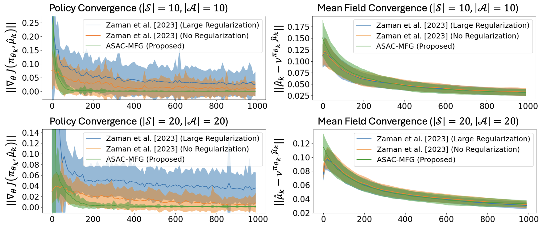
Figure 3: Algorithm Performance in Synthetic Games. Averaged over 100 trials. First columns shows sub-optimality gap of policy under latest mean field estimate. Second column shows convergence of mean field estimate to mean field induced by latest policy iterate. Large regularization is required for theoretical analyses by Zaman et al. (2023), which manifests in persistent bias.

6 Numerical Simulations

We numerically verify the convergence of the proposed algorithm through simulations on small-scale synthetic MFGs. We consider two environments, first of dimension $|{\cal S}|=|{\cal A}|=10$ and second $|{\cal S}|=|{\cal A}|=20$, both of which have a randomly generated transition kernel and reward function. Due to the unknown equilibria, we measure the convergence of the policy by $\|\nabla_{\theta}J(\pi_{\theta_{k}},\hat{\mu}_{k})\|$ and the convergence of the mean field by $\|\hat{\mu}_{k}-\nu^{\pi_{k},\hat{\mu}_{k}}\|$ as a proxy for $\|\hat{\mu}_{k}-\mu^{\star}(\pi_{\theta_{k}})\|$.

We compare ASAC-MFG with the algorithm proposed in Zaman et al. (2020) as the information oracles are similar and enables a fair comparison. We consider two variations of their algorithm: 1) with regularization large enough that the contraction assumption holds, and 2) with regularization set to 0 which breaks the assumption. The environments do not satisfy Assumption 4 with $\Delta=0$, so the theoretical result in Sec.4.1 guarantees the convergence of ASAC-MFG up to an error proportional to $\Delta$. As shown in Figure 3, all algorithms have their mean field iterates converge to the mean field induced by the latest policy iterate, while the convergence of the policy varies. For the considered examples, ASAC-MFG and Zaman et al. (2023) with no regularization exhibit convergence to a global MFE. However, ASAC-MFG converges at a faster rate, which we believe can be attributed to the single-loop updates as well as the fact that our work still enjoys convergence guarantees on this problem (though not to the exactly optimal solution) while Zaman et al. (2023) under no regularization loses any guarantee. ASAC-MFG is also superior in that the convergence path has a much smaller variance. The blue curve in Figure 3 shows that while Zaman et al. (2023) with sufficiently large regularization may converge to a solution of the regularized problem, the bias caused by the large regularization prevents it from finding an equilibrium of the original game.

7 Conclusion

We made several important contributions to the literature on MFGs that are worth re-emphasizing: (i) We proposed a fast policy optimization algorithm for solving MFGs. Being the first of its kind, the algorithm is single loop and uses a single trajectory of continuously generated samples. The analysis is novel, and the convergence results are established under weaker conditions. (ii) We identify a class of MFGs – satisfying a novel herding condition – that can be optimally solved by the proposed algorithm. This expands the class of solvable MFGs, which for the first time is known to include MFGs with more than one equilibrium. (iii) We showed that the current analysis for actor-critic algorithms in average-reward MDPs requires an assumption that is impossible to hold. By recognizing that a MFG reduces to a standard MDP with transition kernal and reward function independent of the mean field, we showed that our main theoretical results lead to a finite-time analysis of an actor-critic algorithm for average-reward MDPs that achieves the state-of-the-art complexity without unrealistic assumptions.

Disclaimer

This paper was prepared for informational purposes [“in part” if the work is collaborative with external partners] by the Artificial Intelligence Research group of JPMorgan Chase & Co. and its affiliates (”JP Morgan”) and is not a product of the Research Department of JP Morgan. JP Morgan makes no representation and warranty whatsoever and disclaims all liability, for the completeness, accuracy or reliability of the information contained herein. This document is not intended as investment research or investment advice, or a recommendation, offer or solicitation for the purchase or sale of any security, financial instrument, financial product or service, or to be used in any way for evaluating the merits of participating in any transaction, and shall not constitute a solicitation under any jurisdiction or to any person, if such solicitation under such jurisdiction or to such person would be unlawful.

Appendix A Notations and Frequently Used Identities

We first introduce a few more shorthand notations frequently used in the analysis. First, we define

$$\begin{aligned} F(\theta,V,\mu,s,a,s^{\prime})&\triangleq(r(s,a,\mu)+V(s^{\prime})-V(s))\nabla_{\theta}\log\pi_{\theta}(a\mid s),\\ G^{V}(V,J,\mu,s,a,s^{\prime})&\triangleq(r(s,a,\mu)-J+V(s^{\prime})-V(s))e_{s},\\ G^{J}(J,\mu,s,a)&\triangleq c_{J}(r(s,a,\mu)-J),\\ G(V,J,\mu,s,a,s^{\prime})&\triangleq\left[\begin{array}[]{c}G^{V}(V,J,\mu,s,a,s^{\prime})\\ G^{J}(J,\mu,s,a)\end{array}\right]=\left[\begin{array}[]{c}(r(s,a,\mu)-J+V(s^{\prime})-V(s))e_{s}\\ c_{J}(r(s,a,\mu)-J)\end{array}\right],\\ H(\mu,s)&\triangleq e_{s}-\mu.\end{aligned}$$ (30)

Then, the update of $f_{k}$, $g_{k}^{V}$, $g_{k}^{J}$, and $h_{k}$ in Algorithm 1 can be alternatively expressed as

$$f_{k+1}=(1-\lambda_{k})f_{k}+\lambda_{k}F(\theta_{k},\hat{V}_{k},\hat{\mu}_{k},s_{k},a_{k},s_{k+1}),$$

$$g_{k+1}^{V}=(1-\lambda_{k})g_{k}^{V}+\lambda_{k}G^{V}(\hat{V}_{k},\hat{J}_{k},\hat{\mu}_{k},s_{k},a_{k},s_{k+1}),$$

$$g_{k+1}^{J}=(1-\lambda_{k})g_{k}^{J}+\lambda_{k}G^{J}(\hat{J}_{k},\hat{\mu}_{k},s_{k},a_{k}),$$

$$h_{k+1}=(1-\lambda_{k})h_{k}+\lambda_{k}H(\hat{\mu}_{k},s_{k}).$$

Denote $g_{k}=[(g_{k}^{V})^{\top},g_{k}^{J}]^{\top}$. The update of $g_{k}$ is

$$g_{k+1}=\left[\begin{array}[]{c}g_{k+1}^{V}\\ g_{k+1}^{J}\end{array}\right]=(1-\lambda_{k})g_{k}+\lambda_{k}G(\hat{V}_{k},\hat{J}_{k},\hat{\mu}_{k},s_{k},a_{k},s_{k+1}).$$

We also define

$$\begin{aligned} \bar{F}(\theta,V,\mu)&\triangleq\mathbb{E}_{s\sim\nu^{\pi_{\theta},\,\mu},a\sim\pi_{\theta}(\cdot\mid s),s^{\prime}\sim{\cal P}(\cdot\mid s,a,\mu)}[F(\theta,V,\mu,s,a,s^{\prime})],\\ \bar{G}^{V}(\theta,V,J,\mu)&\triangleq\mathbb{E}_{s\sim\nu^{\pi_{\theta},\,\mu},a\sim\pi_{\theta}(\cdot\mid s),s^{\prime}\sim{\cal P}(\cdot\mid s,a,\mu)}[G^{V}(V,J,\mu,s,a,s^{\prime})],\\ \bar{G}^{J}(\theta,J,\mu)&\triangleq\mathbb{E}_{s\sim\nu^{\pi_{\theta},\,\mu},a\sim\pi_{\theta}(\cdot\mid s)}[G^{J}(J,\mu,s,a)],\\ \bar{G}(\theta,V,J,\mu)&\triangleq\mathbb{E}_{s\sim\nu^{\pi_{\theta},\,\mu},a\sim\pi_{\theta}(\cdot\mid s),s^{\prime}\sim{\cal P}(\cdot\mid s,a,\mu)}[G(V,J,\mu,s,a,s^{\prime})]=\left[\begin{array}[]{c}\bar{G}^{V}(\theta,V,J,\mu)\\ \bar{G}^{J}(\theta,J,\mu)\end{array}\right],\\ \bar{H}(\theta,\mu)&\triangleq\mathbb{E}_{s\sim\nu^{\pi_{\theta},\,\mu}}[H(\mu,s)]=\mathbb{E}_{s\sim\nu^{\pi_{\theta},\,\mu}}[e_{s}-\mu].\end{aligned}$$ (31)

We measure the convergence of auxiliary variables $f_{k}$, $g_{k}^{V}$, $g_{k}^{J}$, and $h_{k}$ by

$$\Delta f_{k}\triangleq f_{k}-\bar{F}(\theta_{k},\hat{V}_{k},\hat{\mu}_{k}),\quad\Delta g_{k}^{V}\triangleq g_{k}^{V}-\bar{G}^{V}(\theta_{k},\hat{V}_{k},\hat{J}_{k},\hat{\mu}_{k}),$$

$$\Delta g_{k}^{J}\triangleq g_{k}^{J}-\bar{G}^{J}(\theta_{k},\hat{J}_{k},\hat{\mu}_{k}),\quad\Delta h_{k}\triangleq h_{k}-\bar{H}(\theta_{k},\hat{\mu}_{k}),$$

and denote

$$\Delta g_{k}=\left[\begin{array}[]{c}\Delta g_{k}^{V}\\ \Delta g_{k}^{J}\end{array}\right]=g_{k}-\bar{G}(\theta_{k},\hat{V}_{k},\hat{J}_{k},\hat{\mu}_{k}).$$

We use $\ell(\pi)$ to denote the cumulative reward collected by policy $\pi$ under the induced mean field $\mu^{\star}(\pi)$

$$\ell(\pi)\triangleq J(\pi,\mu^{\star}(\pi)).$$

This is well-defined since $\mu^{\star}(\pi)$ is unique.

We denote by ${\cal F}_{k}=\{s_{0},a_{0},s_{1},a_{1}\cdots,s_{k},a_{k}\}$ denote the filtration (set of all randomness information) up to iteration $k$.

We use the notation ${\cal P}_{\mu}(s^{\prime}\mid s,a)={\cal P}(s^{\prime}\mid s,a,\mu)$. Under Assumptions 1 and 2, it can be shown using an argument similar to Lemma B.1 of Wu et al. [2020] that there exists a constant $L_{TV}$ depending only on $|{\cal A}|$, $L$, $C_{0}$, and $C_{1}$ such that for all $\pi_{1},\pi_{2},\mu_{1},\mu_{2}$

$$d_{TV}(\nu^{\pi_{1},\,\mu_{1}}\otimes\pi_{1}\otimes{\cal P}_{\mu_{1}},\nu^{\pi_{2},\,\mu_{2}}\otimes\pi_{2}\otimes{\cal P}_{\mu_{2}})\leq L_{TV}(\|\pi_{1}-\pi_{2}\|+\|\mu_{1}-\mu_{2}\|).$$ (32)

Without loss of generality, we assume $L\geq 1$, a condition that we will sometimes use to simplify and combine terms.

A.1 Mixing Time

An immediate consequence of Assumption 1 is that the Markov chain under any policy and mean field has a geometric mixing time.

Definition 2

Consider a Markov chain $\{\hat{s}_{k}\}$ generated according to $\hat{s}_{k}\sim P^{\pi,\,\mu}(\cdot\mid\hat{s}_{k-1})$, for which $\nu^{\pi,\,\mu}$ is the stationary distribution. For any $c>0$, the $c$-mixing time of the Markov chain is

$$\tau^{\pi,\,\mu}(c)\triangleq\min\big{\{}k\in\mathbb{N}:\textstyle\sup_{s}d_{TV}\big{(}\mathbb{P}(\hat{s}_{k}=\cdot\mid\hat{s}_{0}=s),\,\nu^{\pi,\,\mu}(\cdot)\big{)}\leq c\big{\}}.$$

The mixing time measures time for the samples of the Markov chain to approach its stationary distribution in TV distance. We define $\tau_{k}\triangleq\sup_{\pi,\,\mu}\tau^{\pi,\,\mu}(\alpha_{k})$ as the time when the TV distance drops below $\alpha_{k}$, where $\alpha_{k}$ is a step size for the policy parameter update in Algorithm 1. Under Assumption 1, it is obvious that there exists a constant $C$ as a function of $C_{0},C_{1}$ such that

$$\tau_{k}\leq C\log\left(1/\alpha_{k}\right)=C\log(\frac{(k+1)^{1/2}}{\alpha_{0}})=\frac{C}{2}\log(k+1)-C\log(\alpha_{0}).$$

A.2 Supporting Lemmas

The value function $V^{\pi_{\theta},\,\mu}$ is Lipschitz in both $\theta$ and $\mu$, as shown in the lemma below.

Lemma 1

Under Assumption 2, there exist a bounded constant $L_{V}\geq 1$ such that for any policy parameter $\theta_{1},\theta_{2}$ and mean field $\mu_{1},\mu_{2}$, we have

$$\|\Pi_{{\cal E}_{\perp}}(V^{\pi_{\theta_{1}},\,\mu_{1}}-V^{\pi_{\theta_{2}},\,\mu_{2}})\|\leq L_{V}\left(\|\theta_{1}-\theta_{2}\|+\|\mu_{1}-\mu_{2}\|\right),$$

$$\|J(\pi_{\theta_{1}},\,\mu_{1})-J(\pi_{\theta_{2}},\,\mu_{2})\|\leq L_{V}\left(\|\theta_{1}-\theta_{2}\|+\|\mu_{1}-\mu_{2}\|\right),$$

$$\|\nabla_{\theta}J(\pi_{\theta_{1}},\,\mu_{1})-\nabla_{\theta}J(\pi_{\theta_{2}},\,\mu_{2})\|\leq L_{V}\left(\|\theta_{1}-\theta_{2}\|+\|\mu_{1}-\mu_{2}\|\right),$$

$$\|\nabla_{\mu}J(\pi_{\theta_{1}},\,\mu_{1})-\nabla_{\mu}J(\pi_{\theta_{2}},\,\mu_{2})\|\leq L_{V}\left(\|\theta_{1}-\theta_{2}\|+\|\mu_{1}-\mu_{2}\|\right).$$

We establish the boundedness of the operators $F$, $G$, and $H$.

Lemma 2

For any $\theta\in\mathbb{R}^{|{\cal S}||{\cal A}|}$, $V\in\mathbb{R}^{|{\cal S}|}$ with norm bounded by $B_{V}$, $J\in[0,1]$, $\mu\in\Delta_{{\cal S}}$, and $s,a,s^{\prime}$, we have

$$\|F(\theta,V,\mu,s,a,s^{\prime})\|\leq B_{F},\|G(V,J,\mu,s,a,s^{\prime})\|\leq B_{G},\|H(\mu,s)\|\leq B_{H},$$

where $B_{F}=B_{V}+1$, $B_{G}=2(B_{V}+c_{J}+2)$, $B_{H}=2$.

Since $f_{k}$, $g_{k}^{V}$, $g_{k}^{J}$, and $h_{k}$ are simply convex combination with the operators $F$, $G^{V}$, $G^{J}$, and $H$, Lemma 2 implies for all $k$

$$\|f_{k}\|\leq B_{F},\quad\|g_{k}^{V}\|\leq B_{G},\quad|g_{k}^{J}|\leq B_{G},\quad\|h_{k}\|\leq B_{H}.$$

We also establish the Lipschitz continuity of these operators.

Lemma 3

We have for any $\theta_{1},\theta_{2}\in\mathbb{R}^{|{\cal S}||{\cal A}|}$, $\mu_{1},\mu_{2}\in\Delta_{{\cal S}}$, $V_{1},V_{2}\in\mathbb{R}^{|{\cal S}|}$, and $J_{1},J_{2}\in\mathbb{R}$

$$\|\bar{F}(\theta_{1},V_{1},\mu_{1})-\bar{F}(\theta_{2},V_{2},\mu_{2})\|\leq L_{F}\Big{(}\|\theta_{1}-\theta_{2}\|+\|\Pi_{{\cal E}_{\perp}}(V_{1}-V_{2})\|+\|\mu_{1}-\mu_{2}\|\Big{)}$$

$$\|\bar{G}(\theta_{1},V_{1},J_{1},\mu_{1})-\bar{G}(\theta_{2},V_{2},J_{2},\mu_{2})\|$$

$$\hskip 100.0pt\leq L_{G}\Big{(}\|\theta_{1}-\theta_{2}\|+\|\Pi_{{\cal E}_{\perp}}(V_{1}-V_{2})\|+|J_{1}-J_{2}|+\|\mu_{1}-\mu_{2}\|\Big{)},$$

$$\|\bar{H}(\theta_{1},\mu_{1})-\bar{H}(\theta_{2},\mu_{2})\|\leq L_{H}\Big{(}\|\theta_{1}-\theta_{2}\|+\|\mu_{1}-\mu_{2}\|\Big{)},$$

where the constants are $L_{F}=10B_{V}+L+2B_{F}L_{TV}+5$, $L_{G}=2B_{G}L_{TV}+(L+1)(c_{J}+1)+2$, and $L_{H}=L+1$.

As a result of Lemma 3, we can establish the following results that bound the energy of the auxiliary variables $f_{k}$, $g_{k}$, and $h_{k}$.

Lemma 4

We have for any $k\geq 0$

$$\|f_{k}\| \leq\|\Delta f_{k}\|+L_{F}\sqrt{\varepsilon_{k}^{V}}+L_{F}(L_{V}+1)\sqrt{\varepsilon_{k}^{\mu}}+\sqrt{\varepsilon_{k}^{\pi}},$$

$$\|g_{k}\| \leq\|\Delta g_{k}\|+L_{G}\sqrt{\varepsilon_{k}^{V}}+L_{G}\sqrt{\varepsilon_{k}^{J}},$$

$$\|h_{k}\| \leq\|\Delta h_{k}\|+L_{H}\sqrt{\epsilon_{k}^{\mu}}.$$

Also as a consequence of Assumption 1, the following lemma holds which states that the Bellman backup operator of the value function is almost everywhere contractive (except along the direction of the all-one vector). This lemma is adapted from Zhang et al. [2021a][Lemma 2] and Tsitsiklis and Van Roy [1999][Lemma 7].

Lemma 5

Recall the definition of ${\cal E}_{\perp}$ in Sec.4.1. There exists a constant $\gamma\in(0,1)$ such that for any $\theta,\mu$ and $V\in{\cal E}_{\perp}$

$$V^{\top}\mathbb{E}_{s\sim\nu^{\pi_{\theta},\,\mu},a\sim\pi_{\theta}(\cdot\mid s),s^{\prime}\sim{\cal P}(\cdot\mid s,a,\mu)}[e_{s}(e_{s^{\prime}}-e_{s})^{\top}]V\leq-\gamma\|V\|^{2}.$$

Appendix B Proof of Main Theorem

B.1 Intermediate Results

The proof of Theorem 1 relies critically on the iteration-wise convergence of policy iterate $\theta_{k}$, mean field iterate $\hat{\mu}_{k}$, value function estimate $\hat{V}_{k}$, $\hat{J}_{k}$, and auxiliary variables $f_{k}$, $h_{k}$, and $g_{k}$, which we bound individually in the propositions below.

B.1.1 Convergence of Policy Iterate

Proposition 1

Under Assumptions 1-2, we have

$$\ell(\pi_{\theta_{k}})-\ell(\pi_{\theta_{k+1}}) \leq-\frac{(1+\rho)\alpha_{k}}{2}\varepsilon_{k}^{\pi}+(1+\rho)\alpha_{k}\|\Delta f_{k}\|^{2}$$

$$\hskip 20.0pt+(1+\rho)L_{F}^{2}\alpha_{k}(\varepsilon_{k}^{V}+\varepsilon_{k}^{\mu})+\frac{(1+\rho)L_{V}B_{F}^{2}\alpha_{k}^{2}}{2}+B_{F}\alpha_{k}\Delta.$$

Proposition 2

Under Assumptions 1-2, we have for all $k\geq\tau_{k}$

$$\mathbb{E}[\|\Delta f_{k+1}\|^{2}]$$

$$\leq(1-\lambda_{k})\mathbb{E}[\|\Delta f_{k}\|^{2}]+(-\frac{\lambda_{k}}{2}+\lambda_{k}^{2}+\frac{48L_{F}^{2}\alpha_{k}^{2}}{\lambda_{k}})\mathbb{E}[\|\Delta f_{k}\|^{2}]$$

$$\hskip 20.0pt+\frac{36L_{F}^{2}\beta_{k}^{2}}{\lambda_{k}}\mathbb{E}[\|\Delta g_{k}\|^{2}]+\frac{24L_{F}^{2}L_{H}^{2}\xi_{k}^{2}}{\lambda_{k}}\mathbb{E}[\|\Delta h_{k}\|^{2}]+\frac{48L_{F}^{2}\alpha_{k}^{2}}{\lambda_{k}}\mathbb{E}[\varepsilon_{k}^{\pi}]+\frac{216L_{F}^{4}L_{V}^{2}\xi_{k}^{2}}{\lambda_{k}}\mathbb{E}[\varepsilon_{k}^{\mu}]$$

$$\hskip 20.0pt+\frac{96L_{F}^{4}L_{G}^{2}\beta_{k}^{2}}{\lambda_{k}}\mathbb{E}[\varepsilon_{k}^{V}]+\frac{48L_{F}^{2}L_{G}^{2}\beta_{k}^{2}}{\lambda_{k}}\mathbb{E}[\varepsilon_{k}^{J}]+(28L+2|{\cal A}|)L_{F}L_{TV}B_{F}^{3}B_{G}B_{H}^{2}\tau_{k}^{2}\lambda_{k}\lambda_{k-\tau_{k}}.$$

The proofs of Propositions 1 and 2 can be found in Sec.D.1 and D.2.

B.1.2 Convergence of Mean Field Estimate

Proposition 3

Under Assumptions 1-3, we have for all $k$

$$\varepsilon_{k+1}^{\mu}\leq(1-\frac{(1-\delta)\xi_{k}}{8})\varepsilon_{k}^{\mu}+\frac{8\xi_{k}}{1-\delta}\|\Delta h_{k}\|^{2}+\frac{32L^{2}\alpha_{k}^{2}}{(1-\delta)\xi_{k}}\left(\|\Delta f_{k}\|^{2}+L_{F}^{2}\varepsilon_{k}^{V}+\varepsilon_{k}^{\pi}\right)+9L^{2}B_{F}^{2}B_{H}^{2}\xi_{k}^{2}.$$

Proposition 4

Under Assumptions 1-2, we have for all $k\geq\tau_{k}$

$$\mathbb{E}[\|\Delta h_{k+1}\|^{2}]$$

$$\leq(1-\lambda_{k})\mathbb{E}[\|\Delta h_{k}\|^{2}]+(-\frac{\lambda_{k}}{2}+\lambda_{k}^{2}+\frac{16L_{H}^{2}\xi_{k}^{2}}{\lambda_{k}})\mathbb{E}[\|\Delta h_{k}\|^{2}]+\frac{32L_{H}^{2}\alpha_{k}^{2}}{\lambda_{k}}\mathbb{E}[\|\Delta f_{k}\|^{2}]$$

$$\hskip 20.0pt+\frac{32L_{H}^{2}L_{F}^{2}\alpha_{k}^{2}}{\lambda_{k}}\mathbb{E}[\varepsilon_{k}^{V}]+\frac{144L_{F}^{2}L_{V}^{2}L_{H}^{4}\xi_{k}^{2}}{\lambda_{k}}\mathbb{E}[\varepsilon_{k}^{\mu}]+\frac{32L_{H}^{2}\alpha_{k}^{2}}{\lambda_{k}}\mathbb{E}[\varepsilon_{k}^{\pi}]+24LB_{F}B_{H}^{2}\tau_{k}^{2}\lambda_{k}\lambda_{k-\tau_{k}}.$$

The proofs of Propositions 3 and 4 can be found in Sec.D.3 and D.4.

B.1.3 Convergence of Valuation Function Estimate

Proposition 5

Under Assumptions 1-2,

$$\varepsilon_{k+1}^{V}+\varepsilon_{k+1}^{J} \leq(1-\frac{\gamma\beta_{k}}{4})(\varepsilon_{k}^{V}+\varepsilon_{k}^{J})+\frac{128L_{V}^{2}\alpha_{k}^{2}}{\gamma\beta_{k}}\|\Delta f_{k}\|^{2}+\frac{8\beta_{k}}{\gamma}\|\Delta g_{k}\|^{2}+\frac{64L_{V}^{2}\xi_{k}^{2}}{\gamma\beta_{k}}\|\Delta h_{k}\|^{2}$$

$$\hskip 20.0pt+\frac{128L_{V}^{2}\alpha_{k}^{2}}{\gamma\beta_{k}}(L_{F}^{2}\varepsilon_{k}^{V}+\varepsilon_{k}^{\pi})+\frac{192L_{V}^{2}\xi_{k}^{2}}{\gamma\beta_{k}}\varepsilon_{k}^{\mu}+28L_{V}^{2}B_{F}^{2}B_{G}^{2}B_{H}^{2}\beta_{k}^{2}.$$

Proposition 6

Under Assumptions 1-2, we have for all $k\geq\tau_{k}$

$$\mathbb{E}[\|\Delta g_{k+1}\|^{2}] \leq(1-\lambda_{k})\mathbb{E}[\|\Delta g_{k}\|^{2}]+(-\frac{\lambda_{k}}{2}+\lambda_{k}^{2}+\frac{72|{\cal S}|L_{G}^{2}\beta_{k}^{2}}{\lambda_{k}})\mathbb{E}[\|\Delta g_{k}\|^{2}]+\frac{48L_{G}^{2}\alpha_{k}^{2}}{\lambda_{k}}\mathbb{E}[\|\Delta f_{k}\|^{2}]$$

$$\hskip 20.0pt+\frac{24L_{G}^{2}\xi_{k}^{2}}{\lambda_{k}}\mathbb{E}[\|\Delta h_{k}\|^{2}]+\frac{48L_{G}^{2}\alpha_{k}^{2}}{\lambda_{k}}\mathbb{E}[\varepsilon_{k}^{\pi}]+\frac{216L_{F}^{2}L_{G}^{2}L_{H}^{2}L_{V}^{2}\xi_{k}^{2}}{\lambda_{k}}\mathbb{E}[\varepsilon_{k}^{\mu}]$$

$$\hskip 20.0pt+\frac{120|{\cal S}|L_{F}^{2}L_{G}^{4}\beta_{k}^{2}}{\lambda_{k}}\mathbb{E}[\varepsilon_{k}^{V}+\varepsilon_{k}^{J}]+(30L+2|{\cal A}|)L_{F}L_{TV}B_{F}B_{G}^{2}B_{H}\tau_{k}^{2}\lambda_{k}\lambda_{k-\tau_{k}}.$$

The proofs of Propositions 5 and 6 can be found in Sec.D.5 and D.6.

B.2 Proof of Theorem 1

The exact requirements on $\lambda_{0},\alpha_{0},\beta_{0},\xi_{0}$ include $c_{J}\geq 1/\gamma$, $\alpha_{0}\leq\xi_{0}\leq\beta_{0}\leq\lambda_{0}$, and

$$\begin{gathered}\alpha_{0}\leq\min\left\{\frac{1}{192(L_{F}^{2}+L_{G}^{2}+L_{H}^{2}+L_{V}^{2}+L^{2}/(1-\delta)+\rho+1)}\lambda_{0},\,C_{\beta}\beta_{0},\,C_{\xi}\xi_{0}\right\},\\ \xi_{0}\leq\min\left\{\frac{\lambda_{0}}{64(L_{H}^{2}L_{F}^{2}+L_{G}^{2}+L_{V}^{2}/\gamma+1/(1-\delta))},\,\frac{(1-\delta)\gamma\beta_{0}}{6912(L_{F}^{4}L_{V}^{2}+L_{F}^{2}L_{G}^{2}L_{H}^{2}L_{V}^{2}+L_{F}^{2}L_{H}^{4}L_{V}^{2}+L_{V}^{2})}\right\},\\ \beta_{0}\leq\min\left\{\frac{\lambda_{0}}{72|{\cal S}|L_{G}^{2}+36L_{F}^{2}+8/\gamma},\,\frac{\gamma}{4L_{G}^{2}},\frac{1-\delta}{2L_{H}^{2}}\right\},\quad\lambda_{0}\leq\frac{1}{4},\end{gathered}$$ (36)

where $C_{\xi}=\min\{\frac{(1-\delta)}{32(1+\rho)L_{F}^{2}},\frac{1-\delta}{4(1+\rho)},\frac{L_{H}}{2L_{F}L_{V}},\frac{1-\delta}{16LL_{F}L_{V}}\}$ and

$$C_{\beta} =\min\Big{\{}\frac{\gamma}{4},\frac{(1+\rho)\gamma}{512(L_{F}^{2}+L_{G}^{2}+L_{H}^{2}+L_{V}^{2}+L^{2}/(1-\delta)},$$

$$\hskip 20.0pt\sqrt{\frac{\gamma}{3456|{\cal S}|(L_{F}^{4}L_{G}^{4}+L_{F}^{2}L_{H}^{2}+(\rho+1)L_{F}^{2}+L_{V}^{2}/\gamma+L^{2}L_{F}^{2}(1-\delta))}},\frac{\gamma}{2(1+\rho)}\Big{\}}.$$

We note that such parameters can always chosen with no conflict in any MFG.

We consider the potential function

$${\cal L}_{k}=\mathbb{E}[\|\Delta f_{k}\|^{2}+\|\Delta g_{k}\|^{2}+\|\Delta h_{k}\|^{2}-\ell(\pi_{\theta_{k}})+\varepsilon_{k}^{V}+\varepsilon_{k}^{J}+\varepsilon_{k}^{\mu}].$$

Collecting the bounds from Propositions 1-6, we have for all $k\geq\tau_{k}$

$${\cal L}_{k+1}$$

$$=\mathbb{E}[\|\Delta f_{k+1}\|^{2}+\|\Delta g_{k+1}\|^{2}+\|\Delta h_{k+1}\|^{2}-\ell(\pi_{\theta_{k+1}})+\varepsilon_{k+1}^{V}+\varepsilon_{k+1}^{J}+\varepsilon_{k+1}^{\mu}]$$

$$\leq(1-\lambda_{k})\mathbb{E}[\|\Delta f_{k}\|^{2}]+(-\frac{\lambda_{k}}{2}+\lambda_{k}^{2}+\frac{48L_{F}^{2}\alpha_{k}^{2}}{\lambda_{k}})\mathbb{E}[\|\Delta f_{k}\|^{2}]$$

$$\hskip 20.0pt+\frac{36L_{F}^{2}\beta_{k}^{2}}{\lambda_{k}}\mathbb{E}[\|\Delta g_{k}\|^{2}]+\frac{24L_{F}^{2}L_{H}^{2}\xi_{k}^{2}}{\lambda_{k}}\mathbb{E}[\|\Delta h_{k}\|^{2}]+\frac{48L_{F}^{2}\alpha_{k}^{2}}{\lambda_{k}}\mathbb{E}[\varepsilon_{k}^{\pi}]+\frac{216L_{F}^{4}L_{V}^{2}\xi_{k}^{2}}{\lambda_{k}}\mathbb{E}[\varepsilon_{k}^{\mu}]$$

$$\hskip 20.0pt+\frac{96L_{F}^{4}L_{G}^{2}\beta_{k}^{2}}{\lambda_{k}}\mathbb{E}[\varepsilon_{k}^{V}]+\frac{48L_{F}^{2}L_{G}^{2}\beta_{k}^{2}}{\lambda_{k}}\mathbb{E}[\varepsilon_{k}^{J}]+(28L+2|{\cal A}|)L_{F}L_{TV}B_{F}^{3}B_{G}B_{H}^{2}\tau_{k}^{2}\lambda_{k}\lambda_{k-\tau_{k}}$$

$$\hskip 20.0pt+(1-\lambda_{k})\mathbb{E}[\|\Delta g_{k}\|^{2}]+(-\frac{\lambda_{k}}{2}+\lambda_{k}^{2}+\frac{72|{\cal S}|L_{G}^{2}\beta_{k}^{2}}{\lambda_{k}})\mathbb{E}[\|\Delta g_{k}\|^{2}]+\frac{48L_{G}^{2}\alpha_{k}^{2}}{\lambda_{k}}\mathbb{E}[\|\Delta f_{k}\|^{2}]$$

$$\hskip 20.0pt+\frac{24L_{G}^{2}\xi_{k}^{2}}{\lambda_{k}}\mathbb{E}[\|\Delta h_{k}\|^{2}]+\frac{48L_{G}^{2}\alpha_{k}^{2}}{\lambda_{k}}\mathbb{E}[\varepsilon_{k}^{\pi}]+\frac{216L_{F}^{2}L_{G}^{2}L_{H}^{2}L_{V}^{2}\xi_{k}^{2}}{\lambda_{k}}\mathbb{E}[\varepsilon_{k}^{\mu}]$$

$$\hskip 20.0pt+\frac{120|{\cal S}|L_{F}^{2}L_{G}^{4}\beta_{k}^{2}}{\lambda_{k}}\mathbb{E}[\varepsilon_{k}^{V}+\varepsilon_{k}^{J}]+(30L+2|{\cal A}|)L_{F}L_{TV}B_{F}B_{G}^{2}B_{H}\tau_{k}^{2}\lambda_{k}\lambda_{k-\tau_{k}}$$

$$\hskip 20.0pt+(1-\lambda_{k})\mathbb{E}[\|\Delta h_{k}\|^{2}]+(-\frac{\lambda_{k}}{2}+\lambda_{k}^{2}+\frac{16L_{H}^{2}\xi_{k}^{2}}{\lambda_{k}})\mathbb{E}[\|\Delta h_{k}\|^{2}]+\frac{32L_{H}^{2}\alpha_{k}^{2}}{\lambda_{k}}\mathbb{E}[\|\Delta f_{k}\|^{2}]$$

$$\hskip 20.0pt+\frac{32L_{H}^{2}L_{F}^{2}\alpha_{k}^{2}}{\lambda_{k}}\mathbb{E}[\varepsilon_{k}^{V}]+\frac{144L_{F}^{2}L_{V}^{2}L_{H}^{4}\xi_{k}^{2}}{\lambda_{k}}\mathbb{E}[\varepsilon_{k}^{\mu}]+\frac{32L_{H}^{2}\alpha_{k}^{2}}{\lambda_{k}}\mathbb{E}[\varepsilon_{k}^{\pi}]+24LB_{F}B_{H}^{2}\tau_{k}^{2}\lambda_{k}\lambda_{k-\tau_{k}}$$

$$\hskip 20.0pt-\mathbb{E}[\ell(\pi_{\theta_{k}})]-\frac{(1+\rho)\alpha_{k}}{2}\mathbb{E}[\varepsilon_{k}^{\pi}]+(1+\rho)\alpha_{k}\mathbb{E}[\|\Delta f_{k}\|^{2}]$$

$$\hskip 20.0pt+(1+\rho)L_{F}^{2}\alpha_{k}\mathbb{E}[\varepsilon_{k}^{V}+\varepsilon_{k}^{\mu}]+\frac{(1+\rho)L_{V}B_{F}^{2}\alpha_{k}^{2}}{2}+B_{F}\alpha_{k}\Delta$$

$$\hskip 20.0pt+(1-\frac{\gamma\beta_{k}}{4})\mathbb{E}[\varepsilon_{k}^{V}+\varepsilon_{k}^{J}]+\frac{128L_{V}^{2}\alpha_{k}^{2}}{\gamma\beta_{k}}\mathbb{E}[\|\Delta f_{k}\|^{2}]+\frac{8\beta_{k}}{\gamma}\mathbb{E}[\|\Delta g_{k}\|^{2}]+\frac{64L_{V}^{2}\xi_{k}^{2}}{\gamma\beta_{k}}\mathbb{E}[\|\Delta h_{k}\|^{2}]$$

$$\hskip 20.0pt+\frac{128L_{V}^{2}\alpha_{k}^{2}}{\gamma\beta_{k}}(L_{F}^{2}\mathbb{E}[\varepsilon_{k}^{V}]+\mathbb{E}[\varepsilon_{k}^{\pi}])+\frac{192L_{V}^{2}\xi_{k}^{2}}{\gamma\beta_{k}}\mathbb{E}[\varepsilon_{k}^{\mu}]+28L_{V}^{2}B_{F}^{2}B_{G}^{2}B_{H}^{2}\beta_{k}^{2}$$

$$\hskip 20.0pt+(1-\frac{(1-\delta)\xi_{k}}{8})\mathbb{E}[\varepsilon_{k}^{\mu}]+\frac{8\xi_{k}}{1-\delta}\mathbb{E}[\|\Delta h_{k}\|^{2}]+\frac{32L^{2}\alpha_{k}^{2}}{(1-\delta)\xi_{k}}\mathbb{E}[\|\Delta f_{k}\|^{2}+L_{F}^{2}\varepsilon_{k}^{V}+\varepsilon_{k}^{\pi}]+9L^{2}B_{F}^{2}B_{H}^{2}\xi_{k}^{2}$$

$$\leq(1-\lambda_{k})\mathbb{E}[\|\Delta f_{k}\|^{2}+\|\Delta g_{k}\|^{2}+\|\Delta h_{k}\|^{2}]-\mathbb{E}[\ell(\pi_{\theta_{k}})]-\frac{(1+\rho)\alpha_{k}}{4}\mathbb{E}[\varepsilon_{k}^{\pi}]$$

$$\hskip 20.0pt+(1-\frac{\gamma\beta_{k}}{8})\mathbb{E}[\varepsilon_{k}^{V}+\varepsilon_{k}^{J}]+(1-\frac{(1-\delta)\xi_{k}}{16})\mathbb{E}[\varepsilon_{k}^{\mu}]+B_{F}\alpha_{k}\Delta$$

$$\hskip 20.0pt+(28L+2|{\cal A}|)L_{F}L_{TV}B_{F}^{3}B_{G}B_{H}^{2}\tau_{k}^{2}\lambda_{k}\lambda_{k-\tau_{k}}+(30L+2|{\cal A}|)L_{F}L_{TV}B_{F}B_{G}^{2}B_{H}\tau_{k}^{2}\lambda_{k}\lambda_{k-\tau_{k}}$$

$$\hskip 20.0pt+24LB_{F}B_{H}^{2}\tau_{k}^{2}\lambda_{k}\lambda_{k-\tau_{k}}+\frac{(1+\rho)L_{V}B_{F}^{2}\alpha_{k}^{2}}{2}+28L_{V}^{2}B_{F}^{2}B_{G}^{2}B_{H}^{2}\beta_{k}^{2}+9L^{2}B_{F}^{2}B_{H}^{2}\xi_{k}^{2}$$

$$\hskip 20.0pt+\underbrace{(-\frac{\lambda_{k}}{2}+\lambda_{k}^{2}+\frac{48L_{F}^{2}\alpha_{k}^{2}}{\lambda_{k}}+\frac{48L_{G}^{2}\alpha_{k}^{2}}{\lambda_{k}}+\frac{32L_{H}^{2}\alpha_{k}^{2}}{\lambda_{k}}+(1+\rho)\alpha_{k}+\frac{128L_{V}^{2}\alpha_{k}^{2}}{\gamma\beta_{k}}+\frac{32L^{2}\alpha_{k}^{2}}{(1-\delta)\lambda_{k}})}_{A_{1}}\mathbb{E}[\|\Delta f_{k}\|^{2}]$$

$$\hskip 20.0pt+\underbrace{(-\frac{\lambda_{k}}{2}+\lambda_{k}^{2}+\frac{72|{\cal S}|L_{G}^{2}\beta_{k}^{2}}{\lambda_{k}}+\frac{36L_{F}^{2}\beta_{k}^{2}}{\lambda_{k}}+\frac{8\beta_{k}}{\gamma})}_{A_{2}}\mathbb{E}[\|\Delta g_{k}\|^{2}]$$

$$\hskip 20.0pt+\underbrace{(-\frac{\lambda_{k}}{2}+\lambda_{k}^{2}+\frac{16L_{H}^{2}\xi_{k}^{2}}{\lambda_{k}}+\frac{24L_{F}^{2}L_{H}^{2}\xi_{k}^{2}}{\lambda_{k}}+\frac{24L_{G}^{2}\xi_{k}^{2}}{\lambda_{k}}+\frac{64L_{V}^{2}\xi_{k}^{2}}{\gamma\lambda_{k}}+\frac{8\xi_{k}}{1-\delta})}_{A_{3}}\mathbb{E}[\|\Delta h_{k}\|^{2}]$$

$$\hskip 20.0pt+\underbrace{(-\frac{(1+\rho)\alpha_{k}}{4}+\frac{48L_{F}^{2}\alpha_{k}^{2}}{\lambda_{k}}+\frac{48L_{G}^{2}\alpha_{k}^{2}}{\lambda_{k}}+\frac{32L_{H}^{2}\alpha_{k}^{2}}{\lambda_{k}}+\frac{128L_{V}^{2}\alpha_{k}^{2}}{\gamma\beta_{k}}+\frac{32L^{2}\alpha_{k}^{2}}{(1-\delta)\lambda_{k}})}_{A_{4}}\mathbb{E}[\varepsilon_{k}^{\pi}]$$

$$\hskip 20.0pt+\underbrace{(-\frac{\gamma\beta_{k}}{8}+\frac{96L_{F}^{4}L_{G}^{2}\beta_{k}^{2}}{\lambda_{k}}+\frac{120|{\cal S}|L_{F}^{2}L_{G}^{4}\beta_{k}^{2}}{\lambda_{k}}+\frac{32L_{F}^{2}L_{H}^{2}\alpha_{k}^{2}}{\lambda_{k}}+(1+\rho)L_{F}^{2}\alpha_{k}+\frac{128L_{V}^{2}\alpha_{k}^{2}}{\gamma\beta_{k}}+\frac{32L^{2}L_{F}^{2}\alpha_{k}^{2}}{(1-\delta)\lambda_{k}})}_{A_{5}}\mathbb{E}[\varepsilon_{k}^{V}+\varepsilon_{k}^{J}]$$

$$\hskip 20.0pt+\underbrace{(-\frac{(1-\delta)\xi_{k}}{16}+\frac{216L_{F}^{4}L_{V}^{2}\xi_{k}^{2}}{\lambda_{k}}+\frac{216L_{F}^{2}L_{G}^{2}L_{H}^{2}L_{V}^{2}\xi_{k}^{2}}{\lambda_{k}}+\frac{144L_{F}^{2}L_{H}^{4}L_{V}^{2}\xi_{k}^{2}}{\lambda_{k}}+(1+\rho)L_{F}^{2}\alpha_{k}+\frac{192L_{V}^{2}\xi_{k}^{2}}{\gamma\beta_{k}})}_{A_{6}}\mathbb{E}[\varepsilon_{k}^{\mu}].$$ (37)

We show that the terms $A_{1}$-$A_{6}$ are all non-positive under the step size conditions in (36). First, under the step size condition $\alpha_{k}\leq\frac{\gamma}{4}\beta_{k}$, $\lambda_{k}\leq 1/4$, and $\alpha_{k}\leq(192(L_{F}^{2}+L_{G}^{2}+L_{H}^{2}+L_{V}^{2}+L^{2}/(1-\delta)+\rho+1))^{-1}\lambda_{k}$

$$A_{1} =-\frac{\lambda_{k}}{2}+\lambda_{k}^{2}+\frac{48L_{F}^{2}\alpha_{k}^{2}}{\lambda_{k}}+\frac{48L_{G}^{2}\alpha_{k}^{2}}{\lambda_{k}}+\frac{32L_{H}^{2}\alpha_{k}^{2}}{\lambda_{k}}+(1+\rho)\alpha_{k}+\frac{128L_{V}^{2}\alpha_{k}^{2}}{\gamma\beta_{k}}+\frac{32L^{2}\alpha_{k}^{2}}{(1-\delta)\lambda_{k}}$$

$$\leq-\frac{\lambda_{k}}{4}+\frac{48(L_{F}^{2}+L_{G}^{2}+L_{H}^{2}+L^{2}/(1-\delta))\alpha_{k}^{2}}{\lambda_{k}}+(1+\rho)\alpha_{k}+32L_{V}^{2}\alpha_{k}$$

$$\leq-\frac{\lambda_{k}}{4}+48(L_{F}^{2}+L_{G}^{2}+L_{H}^{2}+L_{V}^{2}+L^{2}/(1-\delta)+\rho+1)\alpha_{k}$$

$$\leq 0.$$ (38)

Next, under the step size condition $\lambda_{k}\leq 1/4$ and $\beta_{k}\leq(72|{\cal S}|L_{G}^{2}+36L_{F}^{2}+8/\gamma)^{-1}\lambda_{k}$

$$A_{2} =-\frac{\lambda_{k}}{2}+\lambda_{k}^{2}+\frac{72|{\cal S}|L_{G}^{2}\beta_{k}^{2}}{\lambda_{k}}+\frac{36L_{F}^{2}\beta_{k}^{2}}{\lambda_{k}}+\frac{8\beta_{k}}{\gamma}$$

$$\leq-\frac{\lambda_{k}}{4}+(72|{\cal S}|L_{G}^{2}+36L_{F}^{2}+8/\gamma)\beta_{k}$$

$$\leq 0.$$ (39)

Next, under the step size condition $\lambda_{k}\leq 1/4$ and $\xi_{k}\leq(64(L_{H}^{2}L_{F}^{2}+L_{G}^{2}+L_{V}^{2}/\gamma+1/(1-\delta)))^{-1}\lambda_{k}$

$$A_{3} =-\frac{\lambda_{k}}{2}+\lambda_{k}^{2}+\frac{16L_{H}^{2}\xi_{k}^{2}}{\lambda_{k}}+\frac{24L_{F}^{2}L_{H}^{2}\xi_{k}^{2}}{\lambda_{k}}+\frac{24L_{G}^{2}\xi_{k}^{2}}{\lambda_{k}}+\frac{64L_{V}^{2}\xi_{k}^{2}}{\gamma\lambda_{k}}+\frac{8\xi_{k}}{1-\delta}$$

$$\leq-\frac{\lambda_{k}}{4}+64(L_{H}^{2}L_{F}^{2}+L_{G}^{2}+L_{V}^{2}/\gamma+1/(1-\delta))\xi_{k}$$

$$\leq 0.$$ (40)

Next, we have

$$A_{4} =-\frac{(1+\rho)\alpha_{k}}{4}+\frac{48L_{F}^{2}\alpha_{k}^{2}}{\lambda_{k}}+\frac{48L_{G}^{2}\alpha_{k}^{2}}{\lambda_{k}}+\frac{32L_{H}^{2}\alpha_{k}^{2}}{\lambda_{k}}+\frac{128L_{V}^{2}\alpha_{k}^{2}}{\gamma\beta_{k}}+\frac{32L^{2}\alpha_{k}^{2}}{(1-\delta)\lambda_{k}}$$

$$\leq-\frac{(1+\rho)\alpha_{k}}{4}+\frac{128}{\gamma}(L_{F}^{2}+L_{G}^{2}+L_{H}^{2}+L_{V}^{2}+L^{2}/(1-\delta))\frac{\alpha_{k}^{2}}{\beta_{k}}$$

$$\leq 0,$$ (41)

under the step size condition

$$\alpha_{k}\leq\frac{(1+\rho)\gamma}{512(L_{F}^{2}+L_{G}^{2}+L_{H}^{2}+L_{V}^{2}+L^{2}/(1-\delta)}\beta_{k}.$$

Then,

$$A_{5} =-\frac{\gamma\beta_{k}}{8}+\frac{96L_{F}^{4}L_{G}^{2}\beta_{k}^{2}}{\lambda_{k}}+\frac{120|{\cal S}|L_{F}^{2}L_{G}^{4}\beta_{k}^{2}}{\lambda_{k}}+\frac{32L_{F}^{2}L_{H}^{2}\alpha_{k}^{2}}{\lambda_{k}}$$

$$\hskip 20.0pt+(1+\rho)L_{F}^{2}\alpha_{k}+\frac{128L_{V}^{2}\alpha_{k}^{2}}{\gamma\beta_{k}}+\frac{32L^{2}L_{F}^{2}\alpha_{k}^{2}}{(1-\delta)\lambda_{k}}$$

$$\leq-\frac{\gamma\beta_{k}}{8}+432|{\cal S}|(L_{F}^{4}L_{G}^{4}+L_{F}^{2}L_{H}^{2}+(\rho+1)L_{F}^{2}+L_{V}^{2}/\gamma+L^{2}L_{F}^{2}(1-\delta))\frac{\alpha_{k}^{2}}{\beta_{k}}$$

$$\leq 0,$$ (42)

due to the condition

$$\alpha_{k}\leq\sqrt{\frac{\gamma}{3456|{\cal S}|(L_{F}^{4}L_{G}^{4}+L_{F}^{2}L_{H}^{2}+(\rho+1)L_{F}^{2}+L_{V}^{2}/\gamma+L^{2}L_{F}^{2}(1-\delta))}}\beta_{k}.$$

Finally, as a result of $\alpha_{k}\leq\frac{(1-\delta)}{32(1+\rho)L_{F}^{2}}\xi_{k}$ and $\xi_{k}\leq\frac{(1-\delta)\gamma}{6912(L_{F}^{4}L_{V}^{2}+L_{F}^{2}L_{G}^{2}L_{H}^{2}L_{V}^{2}+L_{F}^{2}L_{H}^{4}L_{V}^{2}+L_{V}^{2})}\beta_{k}$

$$A_{6} =-\frac{(1-\delta)\xi_{k}}{16}+\frac{216L_{F}^{4}L_{V}^{2}\xi_{k}^{2}}{\lambda_{k}}+\frac{216L_{F}^{2}L_{G}^{2}L_{H}^{2}L_{V}^{2}\xi_{k}^{2}}{\lambda_{k}}$$

$$\hskip 20.0pt+\frac{144L_{F}^{2}L_{H}^{4}L_{V}^{2}\xi_{k}^{2}}{\lambda_{k}}+(1+\rho)L_{F}^{2}\alpha_{k}+\frac{192L_{V}^{2}\xi_{k}^{2}}{\gamma\beta_{k}}$$

$$\leq-\frac{(1-\delta)\xi_{k}}{32}+\frac{216}{\gamma}(L_{F}^{4}L_{V}^{2}+L_{F}^{2}L_{G}^{2}L_{H}^{2}L_{V}^{2}+L_{F}^{2}L_{H}^{4}L_{V}^{2}+L_{V}^{2})\frac{\xi_{k}^{2}}{\beta_{k}}$$

$$\leq 0.$$ (43)

Plugging (38)-(43) into (37), we have for all $k\geq\tau_{k}$

$${\cal L}_{k+1}$$

$$\leq(1-\lambda_{k})\mathbb{E}[\|\Delta f_{k}\|^{2}+\|\Delta g_{k}\|^{2}+\|\Delta h_{k}\|^{2}]-\mathbb{E}[\ell(\pi_{\theta_{k}})]-\frac{(1+\rho)\alpha_{k}}{4}\mathbb{E}[\varepsilon_{k}^{\pi}]$$

$$\hskip 20.0pt+(1-\frac{\gamma\beta_{k}}{8})\mathbb{E}[\varepsilon_{k}^{V}+\varepsilon_{k}^{J}]+(1-\frac{(1-\delta)\xi_{k}}{16})\mathbb{E}[\varepsilon_{k}^{\mu}]+B_{F}\alpha_{k}\Delta$$

$$\hskip 20.0pt+(28L+2|{\cal A}|)L_{F}L_{TV}B_{F}^{3}B_{G}B_{H}^{2}\tau_{k}^{2}\lambda_{k}\lambda_{k-\tau_{k}}+(30L+2|{\cal A}|)L_{F}L_{TV}B_{F}B_{G}^{2}B_{H}\tau_{k}^{2}\lambda_{k}\lambda_{k-\tau_{k}}$$

$$\hskip 20.0pt+24LB_{F}B_{H}^{2}\tau_{k}^{2}\lambda_{k}\lambda_{k-\tau_{k}}+\frac{(1+\rho)L_{V}B_{F}^{2}\alpha_{k}^{2}}{2}+28L_{V}^{2}B_{F}^{2}B_{G}^{2}B_{H}^{2}\beta_{k}^{2}+9L^{2}B_{F}^{2}B_{H}^{2}\xi_{k}^{2}$$

$$\leq{\cal L}_{k}-\min\left\{\frac{(1+\rho)\alpha_{k}}{4},\frac{\gamma\beta_{k}}{8},\frac{(1-\delta)\xi_{k}}{16}\right\}\mathbb{E}[\varepsilon_{k}^{\pi}+\varepsilon_{k}^{\mu}+\varepsilon_{k}^{V}+\varepsilon_{k}^{J}]+B_{F}\alpha_{k}\Delta+{\cal O}(\frac{\log^{2}(k+1)}{k+1})$$

$$\leq{\cal L}_{k}-\frac{(1+\rho)\alpha_{k}}{4}\mathbb{E}[\varepsilon_{k}^{\pi}+\varepsilon_{k}^{\mu}+\varepsilon_{k}^{V}+\varepsilon_{k}^{J}]+B_{F}\alpha_{k}\Delta+{\cal O}(\frac{\log^{2}(k+1)}{k+1}),$$ (44)

where the last inequality follows from the step size condition $\alpha_{k}\leq\frac{\gamma}{2(1+\rho)}\beta_{k}$ and $\alpha_{k}\leq\frac{1-\delta}{4(1+\rho)}\xi_{k}$.

Re-arranging the terms and summing over iterations, we have

$$\sum_{t=\tau_{k}}^{k-1}\alpha_{t}\mathbb{E}[\varepsilon_{t}^{\pi}+\varepsilon_{t}^{\mu}+\varepsilon_{t}^{V}+\varepsilon_{t}^{J}] \leq\frac{4}{1+\rho}\sum_{t=\tau_{k}}^{k-1}({\cal L}_{t}-{\cal L}_{t+1})+B_{F}\Delta\sum_{t=\tau_{k}}^{k-1}\alpha_{t}+\sum_{t=\tau_{k}}^{k-1}{\cal O}(\frac{\log^{2}(t+1)}{t+1})$$

$$\leq\frac{4}{1+\rho}({\cal L}_{\tau_{k}}+1)+B_{F}\Delta\sum_{t=\tau_{k}}^{k-1}\alpha_{t}+{\cal O}(\log^{3}(k+1)),$$

where the second inequality follows from $-{\cal L}_{k+1}\leq-\ell(\pi_{\theta_{k+1}})\leq 1$ and the well-known relation that

$$\sum_{t=\tau_{k}}^{k-1}\frac{1}{t+1}\leq\sum_{t=0}^{k-1}\frac{1}{t+1}\leq 2\log(k+1).$$

Due to $\tau_{k}\leq{\cal O}(\log(k+1))$, it is also a standard result that (for example, see Zeng et al. [2024][Lemma 3])

$$\sum_{t=\tau_{k}}^{k-1}\alpha_{t}=\sum_{t=\tau_{k}}^{k-1}\frac{\alpha_{0}}{\sqrt{t+1}}=\Theta(k+1).$$

Dividing both sides of the inequality by $\sum_{t=\tau_{k}}^{k-1}\alpha_{t}$, we get

$$\min_{t<k}\mathbb{E}[\varepsilon_{t}^{\pi}+\varepsilon_{t}^{\mu}+\varepsilon_{t}^{V}+\varepsilon_{t}^{J}] \leq\frac{\sum_{t=\tau_{k}}^{k-1}\alpha_{t}\mathbb{E}[\varepsilon_{t}^{\pi}+\varepsilon_{t}^{\mu}+\varepsilon_{t}^{V}+\varepsilon_{t}^{J}]}{\sum_{t=\tau_{k}}^{k-1}\alpha_{t}}$$

$$\leq{\cal O}(\frac{1}{\sqrt{k+1}})\left(\frac{4}{1+\rho}({\cal L}_{\tau_{k}}+1)+{\cal O}(\log^{3}(k+1))\right)+B_{F}\Delta.$$

Since the updates of all iterates in Algorithm 1 are bounded, ${\cal L}_{\tau_{k}}\leq{\cal O}(\tau_{k})\leq{\cal O}(\log(k+1))$. As a result, we eventually have

$$\min_{\tau_{k}\leq t<k}\mathbb{E}[\varepsilon_{t}^{\pi}+\varepsilon_{t}^{\mu}+\varepsilon_{t}^{V}+\varepsilon_{t}^{J}]\leq{\cal O}\left(\frac{\log^{3}(k+1)}{\sqrt{k+1}}\right)+{\cal O}(\Delta).$$

$\blacksquare$

Appendix C Proof of Corollaries

C.1 Proof of Corollary 1

As a result of Assumption 5, we have the following gradient domination condition, which is adapted from Lemma 19 of Ganesh et al. [2024].

Lemma 6

Under Assumption 5, we have the following gradient domination condition for any policy parameter $\theta$ and mean field $\mu$

$$\max_{\bar{\pi}}J(\bar{\pi},\mu)-J(\pi_{\theta},\mu)\leq\frac{1}{\sigma}\|\nabla_{\theta}J(\pi_{\theta},\mu)\|.$$

Since $\varepsilon_{t}^{\pi},\varepsilon_{t}^{\mu},\varepsilon_{t}^{V},\varepsilon_{t}^{J}$ are all non-negative, we have

$$\min_{\tau_{k}\leq t<k}\mathbb{E}\left[\|\nabla_{\theta}J(\pi_{\theta_{t}},\mu)\mid_{\mu=\mu^{\star}(\pi_{\theta_{t}})}\|^{2}\right]\leq{\cal O}\left(\frac{\log^{3}(k+1)}{\sqrt{k+1}}\right)+{\cal O}(\Delta)=\widetilde{{\cal O}}\left(\frac{\log^{3}(k+1)}{\sqrt{k+1}}\right)+{\cal O}(\Delta),$$

$$\min_{\tau_{k}\leq t<k}\mathbb{E}[\|\hat{\mu}_{k}-\mu^{\star}(\pi_{\theta_{k}})\|^{2}]\leq{\cal O}\left(\frac{\log^{3}(k+1)}{\sqrt{k+1}}\right)+{\cal O}(\Delta)=\widetilde{{\cal O}}\left(\frac{\log^{3}(k+1)}{\sqrt{k+1}}\right)+{\cal O}(\Delta).$$

Applying Lemma 6 with $\theta=\theta_{t}$ and $\mu=\mu^{\star}(\pi_{\theta_{t}})$,

$$\max_{\pi}J(\pi,\mu^{\star}(\pi_{\theta_{t}}))-J(\pi_{\theta},\mu^{\star}(\pi_{\theta_{t}}))\leq\frac{1}{\sigma}\|\nabla_{\theta}J(\pi_{\theta_{t}},\mu)\mid_{\mu=\mu^{\star}(\pi_{\theta_{t}})}\|.$$

By Jensen’s inequality,

$$\left(\min_{\tau_{k}\leq t<k}\mathbb{E}\left[\max_{\pi}J(\pi,\mu^{\star}(\pi_{\theta_{t}}))-J(\pi_{\theta_{t}},\mu^{\star}(\pi_{\theta_{t}}))\right]\right)^{2}$$

$$\leq\min_{\tau_{k}\leq t<k}\mathbb{E}\left[\left(\max_{\pi}J(\pi,\mu^{\star}(\pi_{\theta_{t}}))-J(\pi_{\theta_{t}},\mu^{\star}(\pi_{\theta_{t}}))\right)^{2}\right]$$

$$\leq\frac{1}{\sigma^{2}}\min_{\tau_{k}\leq t<k}\mathbb{E}\left[\|\nabla_{\theta}J(\pi_{\theta_{t}},\mu)\mid_{\mu=\mu^{\star}(\pi_{\theta_{t}})}\|^{2}\right]$$

$$\leq\widetilde{{\cal O}}\left(\frac{1}{\sqrt{k+1}}\right)+{\cal O}(\Delta).$$

Taking square root on both sides of this inequality leads to the claimed result on the convergence of the policy.

Similarly, we have

$$\min_{\tau_{k}\leq t<k}\mathbb{E}[\|\hat{\mu}_{k}-\mu^{\star}(\pi_{\theta_{k}})\|] \leq\sqrt{\min_{\tau_{k}\leq t<k}\mathbb{E}[\|\hat{\mu}_{k}-\mu^{\star}(\pi_{\theta_{k}})\|^{2}]}$$

$$\leq\sqrt{\widetilde{{\cal O}}\left(\frac{\log^{3}(k+1)}{\sqrt{k+1}}\right)+{\cal O}(\Delta)}$$

$$\leq\widetilde{{\cal O}}\left(\frac{1}{(k+1)^{1/4}}\right)+{\cal O}(\sqrt{\Delta}).$$

$\blacksquare$

C.2 Proof of Corollary 2

In the context of single-agent MDP we define

$$\varepsilon_{k}^{\pi}=\|\nabla_{\theta}J_{\text{MDP}}(\pi_{\theta_{k}})\|^{2},\quad\varepsilon_{k}^{V}=\|\Pi_{{\cal E}_{\perp}}(\hat{V}_{k}-V_{MDP}^{\pi_{\theta_{k}}})\|^{2},\quad\varepsilon_{k}^{J}=(\hat{J}_{k}-J_{\text{MDP}}(\pi_{\theta_{k}}))^{2}.$$

Theorem 1 implies that

$$\min_{\tau_{k}\leq t<k}\mathbb{E}[\varepsilon_{t}^{\pi}+\varepsilon_{t}^{V}+\varepsilon_{t}^{J}]\leq{\cal O}\left(\frac{\log^{3}(k+1)}{\sqrt{k+1}}\right)+{\cal O}(\Delta).$$

As neither the transition kernel nor the reward function depends on the mean field, Assumption 4 is meaningless, or equivalently, it trivially holds with $\rho=\Delta=0$. Therefore, the claimed result holds by recognizing that $\varepsilon_{k}^{V}$ and $\varepsilon_{k}^{J}$ are non-negative for any $k$.

$\blacksquare$

Appendix D Proof of Propositions

D.1 Proof of Proposition 1

By the $L_{V}$-Lipschitz continuity of the function $J$

$$J(\pi_{\theta_{k}},\mu^{\star}(\pi_{\theta_{k}}))-J(\pi_{\theta_{k+1}},\mu^{\star}(\pi_{\theta_{k}}))$$

$$\leq-\langle\nabla_{\theta}J(\pi_{\theta_{k}},\mu)\mid_{\mu=\mu^{\star}(\pi_{\theta_{k}})},\theta_{k+1}-\theta_{k}\rangle+\frac{L_{V}}{2}\|\theta_{k+1}-\theta_{k}\|^{2}$$

$$=-\alpha_{k}\langle\nabla_{\theta}J(\pi_{\theta_{k}},\mu)\mid_{\mu=\mu^{\star}(\pi_{\theta_{k}})},f_{k}\rangle+\frac{L_{V}\alpha_{k}^{2}}{2}\|f_{k}\|^{2}$$

$$=-\alpha_{k}\langle\nabla_{\theta}J(\pi_{\theta_{k}},\mu)\mid_{\mu=\mu^{\star}(\pi_{\theta_{k}})},\Delta f_{k}\rangle-\alpha_{k}\langle\nabla_{\theta}J(\pi_{\theta_{k}},\mu)\mid_{\mu=\mu^{\star}(\pi_{\theta_{k}})},\bar{F}(\theta_{k},\hat{V}_{k},\hat{\mu}_{k})\rangle+\frac{L_{V}\alpha_{k}^{2}}{2}\|f_{k}\|^{2}$$

$$=-\alpha_{k}\langle\nabla_{\theta}J(\pi_{\theta_{k}},\mu)\mid_{\mu=\mu^{\star}(\pi_{\theta_{k}})},\Delta f_{k}\rangle-\alpha_{k}\|\nabla_{\theta}J(\pi_{\theta_{k}},\mu)\mid_{\mu=\mu^{\star}(\pi_{\theta_{k}})}\|^{2}$$

$$\hskip 20.0pt+\alpha_{k}\langle\nabla_{\theta}J(\pi_{\theta_{k}},\mu)\mid_{\mu=\mu^{\star}(\pi_{\theta_{k}})},\bar{F}(\theta_{k},V^{\pi_{\theta_{k}},\,\mu^{\star}(\pi_{\theta_{k}})},\mu^{\star}(\pi_{\theta_{k}}))-\bar{F}(\theta_{k},\hat{V}_{k},\hat{\mu}_{k})\rangle+\frac{L_{V}\alpha_{k}^{2}}{2}\|f_{k}\|^{2}$$

$$\leq-\alpha_{k}\|\nabla_{\theta}J(\pi_{\theta_{k}},\mu)\mid_{\mu=\mu^{\star}(\pi_{\theta_{k}})}\|^{2}-\alpha_{k}\langle\nabla_{\theta}J(\pi_{\theta_{k}},\mu)\mid_{\mu=\mu^{\star}(\pi_{\theta_{k}})},\Delta f_{k}\rangle$$

$$\hskip 20.0pt+\alpha_{k}\langle\nabla_{\theta}J(\pi_{\theta_{k}},\mu)\mid_{\mu=\mu^{\star}(\pi_{\theta_{k}})},\bar{F}(\theta_{k},V^{\pi_{\theta_{k}},\,\mu^{\star}(\pi_{\theta_{k}})},\mu^{\star}(\pi_{\theta_{k}}))-\bar{F}(\theta_{k},\hat{V}_{k},\hat{\mu}_{k})\rangle+\frac{L_{V}B_{F}^{2}\alpha_{k}^{2}}{2},$$ (45)

where the third equation follows from $\nabla_{\theta}J(\pi_{\theta},\mu)\mid_{\mu=\mu^{\star}(\pi_{\theta})}\,=\bar{F}(\theta,V^{\pi_{\theta},\,\mu^{\star}(\pi_{\theta})},\mu^{\star}(\pi_{\theta}))$ for any $\theta$.

To bound the second term on the right hand side of (45), we use the fact that $\langle\vec{a},\vec{b}\rangle\leq\frac{c}{2}\|\vec{a}\|^{2}+\frac{1}{2c}\|\vec{b}\|^{2}$ for any vectors $\vec{a},\vec{b}$ and scalar $c>0$

$$-\alpha_{k}\langle\nabla_{\theta}J(\pi_{\theta_{k}},\mu)\mid_{\mu=\mu^{\star}(\pi_{\theta_{k}})},\Delta f_{k}\rangle \leq\frac{\alpha_{k}}{4}\|\nabla_{\theta}J(\pi_{\theta_{k}},\mu)\mid_{\mu=\mu^{\star}(\pi_{\theta_{k}})}\|^{2}+\alpha_{k}\|\Delta f_{k}\|^{2}.$$ (46)

Similarly, for the third term of (45), we have

$$\alpha_{k}\langle\nabla_{\theta}J(\pi_{\theta_{k}},\mu)\mid_{\mu=\mu^{\star}(\pi_{\theta_{k}})},\mu^{\star}(\pi_{\theta_{k}}))-\bar{F}(\theta_{k},\hat{V}_{k},\hat{\mu}_{k})\rangle$$

$$\leq\frac{\alpha_{k}}{4}\|\nabla_{\theta}J(\pi_{\theta_{k}},\mu)\mid_{\mu=\mu^{\star}(\pi_{\theta_{k}})}\|^{2}+\alpha_{k}\|\bar{F}(\theta_{k},V^{\pi_{\theta_{k}},\,\mu^{\star}(\pi_{\theta_{k}})},\mu^{\star}(\pi_{\theta_{k}}))-\bar{F}(\theta_{k},\hat{V}_{k},\hat{\mu}_{k})\|^{2}$$

$$\leq\frac{\alpha_{k}}{4}\|\nabla_{\theta}J(\pi_{\theta_{k}},\mu)\mid_{\mu=\mu^{\star}(\pi_{\theta_{k}})}\|^{2}+L_{F}^{2}\alpha_{k}\|\Pi_{{\cal E}_{\perp}}(\hat{V}_{k}-V^{\pi_{\theta_{k}},\mu^{\star}(\pi_{\theta_{k}})})\|^{2}+L_{F}^{2}\alpha_{k}\|\hat{\mu}_{k}-\mu^{\star}(\pi_{\theta_{k}})\|^{2}$$

$$=\frac{\alpha_{k}}{4}\|\nabla_{\theta}J(\pi_{\theta_{k}},\mu)\mid_{\mu=\mu^{\star}(\pi_{\theta_{k}})}\|^{2}+L_{F}^{2}\alpha_{k}(\varepsilon_{k}^{V}+\varepsilon_{k}^{\mu}).$$ (47)

Plugging (46)-(47) into (45), we have

$$J(\pi_{\theta_{k}},\mu^{\star}(\pi_{\theta_{k}}))-J(\pi_{\theta_{k+1}},\mu^{\star}(\pi_{\theta_{k}}))$$

$$\leq-\alpha_{k}\|\nabla_{\theta}J(\pi_{\theta_{k}},\mu)\mid_{\mu=\mu^{\star}(\pi_{\theta_{k}})}\|^{2}-\alpha_{k}\langle\nabla_{\theta}J(\pi_{\theta_{k}},\mu)\mid_{\mu=\mu^{\star}(\pi_{\theta_{k}})},\Delta f_{k}\rangle$$

$$\hskip 20.0pt+\alpha_{k}\langle\nabla_{\theta}J(\pi_{\theta_{k}},\mu)\mid_{\mu=\mu^{\star}(\pi_{\theta_{k}})},\bar{F}(\theta_{k},V^{\pi_{\theta_{k}},\,\mu^{\star}(\pi_{\theta_{k}})},\mu^{\star}(\pi_{\theta_{k}}))-\bar{F}(\theta_{k},\hat{V}_{k},\hat{\mu}_{k})\rangle+\frac{L_{V}B_{F}^{2}\alpha_{k}^{2}}{2}$$

$$\leq-\alpha_{k}\|\nabla_{\theta}J(\pi_{\theta_{k}},\mu)\mid_{\mu=\mu^{\star}(\pi_{\theta_{k}})}\|^{2}+\frac{\alpha_{k}}{4}\|\nabla_{\theta}J(\pi_{\theta_{k}},\mu)\mid_{\mu=\mu^{\star}(\pi_{\theta_{k}})}\|^{2}+\alpha_{k}\|\Delta f_{k}\|^{2}$$

$$\hskip 20.0pt+\frac{\alpha_{k}}{4}\|\nabla_{\theta}J(\pi_{\theta_{k}},\mu)\mid_{\mu=\mu^{\star}(\pi_{\theta_{k}})}\|^{2}+L_{F}^{2}\alpha_{k}(\varepsilon_{k}^{V}+\varepsilon_{k}^{\mu})+\frac{L_{V}B_{F}^{2}\alpha_{k}^{2}}{2}$$

$$\leq-\frac{\alpha_{k}}{2}\|\nabla_{\theta}J(\pi_{\theta_{k}},\mu)\mid_{\mu=\mu^{\star}(\pi_{\theta_{k}})}\|^{2}+\alpha_{k}\|\Delta f_{k}\|^{2}+L_{F}^{2}\alpha_{k}(\varepsilon_{k}^{V}+\varepsilon_{k}^{\mu})+\frac{L_{V}B_{F}^{2}\alpha_{k}^{2}}{2}.$$ (48)

By Assumption 4, we have

$$J(\pi_{\theta_{k+1}},\mu^{\star}(\pi_{\theta_{k}}))-J(\pi_{\theta_{k+1}},\mu^{\star}(\pi_{\theta_{k+1}}))$$

$$\leq\rho\Big{(}J(\pi_{\theta_{k}},\mu^{\star}(\pi_{\theta_{k}}))-J(\pi_{\theta_{k+1}},\mu^{\star}(\pi_{\theta_{k}}))\Big{)}+\Delta\|\theta_{k+1}-\theta_{k}\|$$

$$\leq\rho\big{(}-\frac{\alpha_{k}}{2}\|\nabla_{\theta}J(\pi_{\theta_{k}},\mu)\mid_{\mu=\mu^{\star}(\pi_{\theta_{k}})}\|^{2}+\alpha_{k}\|\Delta f_{k}\|^{2}+L_{F}^{2}\alpha_{k}(\varepsilon_{k}^{V}+\varepsilon_{k}^{\mu})+\frac{L_{V}B_{F}^{2}\alpha_{k}^{2}}{2}\big{)}+B_{F}\alpha_{k}\Delta.$$ (49)

Combining (48) and (49),

$$J(\pi_{\theta_{k}},\mu^{\star}(\pi_{\theta_{k}}))-J(\pi_{\theta_{k+1}},\mu^{\star}(\pi_{\theta_{k+1}}))$$

$$\leq-\frac{\alpha_{k}}{2}\|\nabla_{\theta}J(\pi_{\theta_{k}},\mu)\mid_{\mu=\mu^{\star}(\pi_{\theta_{k}})}\|^{2}+\alpha_{k}\|\Delta f_{k}\|^{2}+L_{F}^{2}\alpha_{k}(\varepsilon_{k}^{V}+\varepsilon_{k}^{\mu})+\frac{L_{V}B_{F}^{2}\alpha_{k}^{2}}{2}$$

$$\hskip 20.0pt+\rho\Big{(}-\frac{\alpha_{k}}{2}\|\nabla_{\theta}J(\pi_{\theta_{k}},\mu)\mid_{\mu=\mu^{\star}(\pi_{\theta_{k}})}\|^{2}+\alpha_{k}\|\Delta f_{k}\|^{2}+L_{F}^{2}\alpha_{k}(\varepsilon_{k}^{V}+\varepsilon_{k}^{\mu})+\frac{L_{V}B_{F}^{2}\alpha_{k}^{2}}{2}\Big{)}$$

$$\hskip 20.0pt+B_{F}\alpha_{k}\Delta$$

$$\leq-\frac{(1+\rho)\alpha_{k}}{2}\|\nabla_{\theta}J(\pi_{\theta_{k}},\mu)\mid_{\mu=\mu^{\star}(\pi_{\theta_{k}})}\|^{2}+(1+\rho)\alpha_{k}\|\Delta f_{k}\|^{2}+(1+\rho)L_{F}^{2}\alpha_{k}(\varepsilon_{k}^{V}+\varepsilon_{k}^{\mu})$$

$$\hskip 20.0pt+\frac{(1+\rho)L_{V}B_{F}^{2}\alpha_{k}^{2}}{2}++B_{F}\alpha_{k}\Delta.$$

$\blacksquare$

D.2 Proof of Proposition 2

The proof of Proposition 2 relies on the lemma below. We defer the proof of the lemma to Sec.E.7.

Lemma 7

We have for all $k\geq\tau_{k}$

$$\mathbb{E}[\langle\Delta f_{k},F(\theta_{k},\hat{V}_{k},\hat{\mu}_{k},s_{k},a_{k},s_{k+1})-\bar{F}(\theta_{k},\hat{V}_{k},\hat{\mu}_{k})\rangle]\leq(20L+2|{\cal A}|)L_{F}L_{TV}B_{F}^{3}B_{G}B_{H}^{2}\tau_{k}^{2}\lambda_{k-\tau_{k}}.$$

By the update rule of $f_{k}$,

$$\Delta f_{k+1} =f_{k+1}-\bar{F}(\theta_{k+1},\hat{V}_{k+1},\hat{\mu}_{k+1})$$

$$=(1-\lambda_{k})f_{k}+\lambda_{k}F(\theta_{k},\hat{V}_{k},\hat{\mu}_{k},s_{k},a_{k},s_{k+1})-\bar{F}(\theta_{k+1},\hat{V}_{k+1},\hat{\mu}_{k+1})$$

$$=(1-\lambda_{k})f_{k}+\lambda_{k}\bar{F}(\theta_{k},\hat{V}_{k},\hat{\mu}_{k})-\bar{F}(\theta_{k+1},\hat{V}_{k+1},\hat{\mu}_{k+1})$$

$$\hskip 20.0pt+\lambda_{k}\Big{(}F(\theta_{k},\hat{V}_{k},\hat{\mu}_{k},s_{k},a_{k},s_{k+1})-\bar{F}(\theta_{k},\hat{V}_{k},\hat{\mu}_{k})\Big{)}$$

$$=(1-\lambda_{k})\Delta f_{k}+\Big{(}\bar{F}(\theta_{k},\hat{V}_{k},\hat{\mu}_{k})-\bar{F}(\theta_{k+1},\hat{V}_{k+1},\hat{\mu}_{k+1})\Big{)}$$

$$\hskip 20.0pt+\lambda_{k}\Big{(}F(\theta_{k},\hat{V}_{k},\hat{\mu}_{k},s_{k},a_{k},s_{k+1})-\bar{F}(\theta_{k},\hat{V}_{k},\hat{\mu}_{k})\Big{)}.$$

Taking the norm, we have

$$\|\Delta f_{k+1}\|^{2}$$

$$=(1-\lambda_{k})^{2}\|\Delta f_{k}\|^{2}+\|\bar{F}(\theta_{k},\hat{V}_{k},\hat{\mu}_{k})-\bar{F}(\theta_{k+1},\hat{V}_{k+1},\hat{\mu}_{k+1})\|^{2}$$

$$\hskip 20.0pt+\lambda_{k}^{2}\|F(\theta_{k},\hat{V}_{k},\hat{\mu}_{k},s_{k},a_{k},s_{k+1})-\bar{F}(\theta_{k},\hat{V}_{k},\hat{\mu}_{k})\|^{2}$$

$$\hskip 20.0pt+(1-\lambda_{k})\langle\Delta f_{k},\bar{F}(\theta_{k},\hat{V}_{k},\hat{\mu}_{k})-\bar{F}(\theta_{k+1},\hat{V}_{k+1},\hat{\mu}_{k+1})\rangle$$

$$\hskip 20.0pt+(1-\lambda_{k})\lambda_{k}\langle\Delta f_{k},F(\theta_{k},\hat{V}_{k},\hat{\mu}_{k},s_{k},a_{k},s_{k+1})-\bar{F}(\theta_{k},\hat{V}_{k},\hat{\mu}_{k})\rangle$$

$$\hskip 20.0pt+\lambda_{k}\langle\bar{F}(\theta_{k},\hat{V}_{k},\hat{\mu}_{k})-\bar{F}(\theta_{k+1},\hat{V}_{k+1},\hat{\mu}_{k+1}),F(\theta_{k},\hat{V}_{k},\hat{\mu}_{k},s_{k},a_{k},s_{k+1})-\bar{F}(\theta_{k},\hat{V}_{k},\hat{\mu}_{k})\rangle$$

$$\leq(1-\lambda_{k})^{2}\|\Delta f_{k}\|^{2}+2\|\bar{F}(\theta_{k},\hat{V}_{k},\hat{\mu}_{k})-\bar{F}(\theta_{k+1},\hat{V}_{k+1},\hat{\mu}_{k+1})\|^{2}$$

$$\hskip 20.0pt+2\lambda_{k}^{2}\|F(\theta_{k},\hat{V}_{k},\hat{\mu}_{k},s_{k},a_{k},s_{k+1})-\bar{F}(\theta_{k},\hat{V}_{k},\hat{\mu}_{k})\|^{2}$$

$$\hskip 20.0pt+\frac{\lambda_{k}}{2}\|\Delta f_{k}\|^{2}+\frac{2}{\lambda_{k}}\|\bar{F}(\theta_{k},\hat{V}_{k},\hat{\mu}_{k})-\bar{F}(\theta_{k+1},\hat{V}_{k+1},\hat{\mu}_{k+1})\|^{2}$$

$$\hskip 20.0pt+(1-\lambda_{k})\lambda_{k}\langle\Delta f_{k},F(\theta_{k},\hat{V}_{k},\hat{\mu}_{k},s_{k},a_{k},s_{k+1})-\bar{F}(\theta_{k},\hat{V}_{k},\hat{\mu}_{k})\rangle$$

$$\leq(1-\lambda_{k})\|\Delta f_{k}\|^{2}+(-\frac{\lambda_{k}}{2}+\lambda_{k}^{2})\|\Delta f_{k}\|^{2}+\frac{4}{\lambda_{k}}\|\bar{F}(\theta_{k},\hat{V}_{k},\hat{\mu}_{k})-\bar{F}(\theta_{k+1},\hat{V}_{k+1},\hat{\mu}_{k+1})\|^{2}$$

$$\hskip 20.0pt+8B_{F}^{2}\lambda_{k}^{2}+(1-\lambda_{k})\lambda_{k}\langle\Delta f_{k},F(\theta_{k},\hat{V}_{k},\hat{\mu}_{k},s_{k},a_{k},s_{k+1})-\bar{F}(\theta_{k},\hat{V}_{k},\hat{\mu}_{k})\rangle,$$ (50)

where the final inequality follows from the step size condition $\lambda_{k}\leq 1$ and the boundedness of operator $F$ which implies

$$\|\bar{F}(\theta_{k},\hat{V}_{k},\hat{\mu}_{k})-\bar{F}(\theta_{k+1},\hat{V}_{k+1},\hat{\mu}_{k+1})\|\leq 2B_{F}.$$

Taking the expectation, we can simplify (50) as

$$\mathbb{E}[\|\Delta f_{k+1}\|^{2}]$$

$$\leq\mathbb{E}\Big{[}(1-\lambda_{k})\|\Delta f_{k}\|^{2}+(-\frac{\lambda_{k}}{2}+\lambda_{k}^{2})\|\Delta f_{k}\|^{2}+\frac{4}{\lambda_{k}}\|\bar{F}(\theta_{k},\hat{V}_{k},\hat{\mu}_{k})-\bar{F}(\theta_{k+1},\hat{V}_{k+1},\hat{\mu}_{k+1})\|^{2}$$

$$\hskip 20.0pt+8B_{F}^{2}\lambda_{k}^{2}+(1-\lambda_{k})\lambda_{k}\langle\Delta f_{k},F(\theta_{k},\hat{V}_{k},\hat{\mu}_{k},s_{k},a_{k},s_{k+1})-\bar{F}(\theta_{k},\hat{V}_{k},\hat{\mu}_{k})\rangle\Big{]}$$

$$\leq(1-\lambda_{k})\mathbb{E}[\|\Delta f_{k}\|^{2}]+(-\frac{\lambda_{k}}{2}+\lambda_{k}^{2})\mathbb{E}[\|\Delta f_{k}\|^{2}]+8B_{F}^{2}\lambda_{k}^{2}$$

$$\hskip 20.0pt+\frac{4L_{F}^{2}}{\lambda_{k}}\mathbb{E}[\left(\|\theta_{k}-\theta_{k+1}\|+\|\hat{V}_{k}-\hat{V}_{k+1}\|+\|\hat{\mu}_{k}-\hat{\mu}_{k+1}\|\right)^{2}]$$

$$\hskip 20.0pt+(1-\lambda_{k})\lambda_{k}\cdot(20L+2|{\cal A}|)L_{F}L_{TV}B_{F}^{3}B_{G}B_{H}^{2}\tau_{k}^{2}\lambda_{k-\tau_{k}}$$

$$\leq(1-\lambda_{k})\mathbb{E}[\|\Delta f_{k}\|^{2}]+(-\frac{\lambda_{k}}{2}+\lambda_{k}^{2})\mathbb{E}[\|\Delta f_{k}\|^{2}]+(28L+2|{\cal A}|)L_{F}L_{TV}B_{F}^{3}B_{G}B_{H}^{2}\tau_{k}^{2}\lambda_{k}\lambda_{k-\tau_{k}}$$

$$\hskip 20.0pt+\frac{4L_{F}^{2}}{\lambda_{k}}\mathbb{E}[\left(\alpha_{k}\|f_{k}\|+\beta_{k}\|g_{k}\|+\xi_{k}\|h_{k}\|\right)^{2}]$$

$$\leq(1-\lambda_{k})\mathbb{E}[\|\Delta f_{k}\|^{2}]+(-\frac{\lambda_{k}}{2}+\lambda_{k}^{2})\mathbb{E}[\|\Delta f_{k}\|^{2}]+(28L+2|{\cal A}|)L_{F}L_{TV}B_{F}^{3}B_{G}B_{H}^{2}\tau_{k}^{2}\lambda_{k}\lambda_{k-\tau_{k}}$$

$$\hskip 20.0pt+\mathbb{E}\Big{[}\frac{12L_{F}^{2}\alpha_{k}}{\lambda_{k}}\left(\|\Delta f_{k}\|+L_{F}\sqrt{\varepsilon_{k}^{V}}+L_{F}(L_{V}+1)\sqrt{\varepsilon_{k}^{\mu}}+\sqrt{\varepsilon_{k}^{\pi}}\right)^{2}$$

$$\hskip 20.0pt+\frac{12L_{F}^{2}\beta_{k}}{\lambda_{k}}\left(\|\Delta g_{k}\|+L_{G}\sqrt{\varepsilon_{k}^{V}}+L_{G}\sqrt{\varepsilon_{k}^{J}}\right)^{2}+\frac{12L_{F}^{2}\xi_{k}}{\lambda_{k}}\left(L_{H}\|\Delta h_{k}\|+\sqrt{\varepsilon_{k}^{\mu}}\right)^{2}\Big{]},$$ (51)

where the second inequality plugs in the result of Lemma 7 and bounds $\|\bar{F}(\theta_{k},\hat{V}_{k},\hat{\mu}_{k})-\bar{F}(\theta_{k+1},\hat{V}_{k+1},\hat{\mu}_{k+1})\|^{2}$ using the Lipschitz condition established in Lemma 3.

The sum of the last three terms can be bounded as

$$\frac{12L_{F}^{2}\alpha_{k}}{\lambda_{k}}\left(\|\Delta f_{k}\|+L_{F}\sqrt{\varepsilon_{k}^{V}}+L_{F}(L_{V}+1)\sqrt{\varepsilon_{k}^{\mu}}+\sqrt{\varepsilon_{k}^{\pi}}\right)^{2}$$

$$\hskip 20.0pt+\frac{12L_{F}^{2}\beta_{k}}{\lambda_{k}}\left(\|\Delta g_{k}\|+L_{G}\sqrt{\varepsilon_{k}^{V}}+L_{G}\sqrt{\varepsilon_{k}^{J}}\right)^{2}+\frac{12L_{F}^{2}\xi_{k}}{\lambda_{k}}\left(L_{H}\|\Delta h_{k}\|+\sqrt{\varepsilon_{k}^{\mu}}\right)^{2}$$

$$\leq\frac{48L_{F}^{2}\alpha_{k}^{2}}{\lambda_{k}}\|\Delta f_{k}\|^{2}+\frac{48L_{F}^{4}\alpha_{k}^{2}}{\lambda_{k}}\varepsilon_{k}^{V}+\frac{192L_{F}^{4}L_{V}^{2}\alpha_{k}^{2}}{\lambda_{k}}\varepsilon_{k}^{\mu}+\frac{48L_{F}^{2}\alpha_{k}^{2}}{\lambda_{k}}\varepsilon_{k}^{\pi}$$

$$\hskip 20.0pt+\frac{36L_{F}^{2}\beta_{k}^{2}}{\lambda_{k}}\|\Delta g_{k}\|^{2}+\frac{48L_{F}^{2}L_{G}^{2}\beta_{k}^{2}}{\lambda_{k}}\varepsilon_{k}^{V}+\frac{48L_{F}^{2}L_{G}^{2}\beta_{k}^{2}}{\lambda_{k}}\varepsilon_{k}^{J}$$

$$\hskip 20.0pt+\frac{24L_{F}^{2}L_{H}^{2}\xi_{k}^{2}}{\lambda_{k}}\|\Delta h_{k}\|^{2}+\frac{24L_{F}^{2}\xi_{k}^{2}}{\lambda_{k}}\varepsilon_{k}^{\mu}$$

$$\leq\frac{48L_{F}^{2}\alpha_{k}^{2}}{\lambda_{k}}\|\Delta f_{k}\|^{2}+\frac{36L_{F}^{2}\beta_{k}^{2}}{\lambda_{k}}\|\Delta g_{k}\|^{2}+\frac{24L_{F}^{2}L_{H}^{2}\xi_{k}^{2}}{\lambda_{k}}\|\Delta h_{k}\|^{2}+\frac{48L_{F}^{2}\alpha_{k}^{2}}{\lambda_{k}}\varepsilon_{k}^{\pi}$$

$$\hskip 20.0pt+\frac{216L_{F}^{4}L_{V}^{2}\xi_{k}^{2}}{\lambda_{k}}\varepsilon_{k}^{\mu}+\frac{96L_{F}^{4}L_{G}^{2}\beta_{k}^{2}}{\lambda_{k}}\varepsilon_{k}^{V}+\frac{48L_{F}^{2}L_{G}^{2}\beta_{k}^{2}}{\lambda_{k}}\varepsilon_{k}^{J}.$$ (52)

Combining (51) and (52), we get

$$\mathbb{E}[\|\Delta f_{k+1}\|^{2}]$$

$$\leq(1-\lambda_{k})\mathbb{E}[\|\Delta f_{k}\|^{2}]+(-\frac{\lambda_{k}}{2}+\lambda_{k}^{2})\mathbb{E}[\|\Delta f_{k}\|^{2}]+(28L+2|{\cal A}|)L_{F}L_{TV}B_{F}^{3}B_{G}B_{H}^{2}\tau_{k}^{2}\lambda_{k}\lambda_{k-\tau_{k}}$$

$$\hskip 20.0pt+\mathbb{E}\Big{[}\frac{48L_{F}^{2}\alpha_{k}^{2}}{\lambda_{k}}\|\Delta f_{k}\|^{2}+\frac{36L_{F}^{2}\beta_{k}^{2}}{\lambda_{k}}\|\Delta g_{k}\|^{2}+\frac{24L_{F}^{2}L_{H}^{2}\xi_{k}^{2}}{\lambda_{k}}\|\Delta h_{k}\|^{2}+\frac{48L_{F}^{2}\alpha_{k}^{2}}{\lambda_{k}}\varepsilon_{k}^{\pi}$$

$$\hskip 20.0pt+\frac{216L_{F}^{4}L_{V}^{2}\xi_{k}^{2}}{\lambda_{k}}\varepsilon_{k}^{\mu}+\frac{96L_{F}^{4}L_{G}^{2}\beta_{k}^{2}}{\lambda_{k}}\varepsilon_{k}^{V}+\frac{48L_{F}^{2}L_{G}^{2}\beta_{k}^{2}}{\lambda_{k}}\varepsilon_{k}^{J}\Big{]}$$

$$=(1-\lambda_{k})\mathbb{E}[\|\Delta f_{k}\|^{2}]+(-\frac{\lambda_{k}}{2}+\lambda_{k}^{2}+\frac{48L_{F}^{2}\alpha_{k}^{2}}{\lambda_{k}})\mathbb{E}[\|\Delta f_{k}\|^{2}]$$

$$\hskip 20.0pt+\frac{36L_{F}^{2}\beta_{k}^{2}}{\lambda_{k}}\mathbb{E}[\|\Delta g_{k}\|^{2}]+\frac{24L_{F}^{2}L_{H}^{2}\xi_{k}^{2}}{\lambda_{k}}\mathbb{E}[\|\Delta h_{k}\|^{2}]+\frac{48L_{F}^{2}\alpha_{k}^{2}}{\lambda_{k}}\mathbb{E}[\varepsilon_{k}^{\pi}]+\frac{216L_{F}^{4}L_{V}^{2}\xi_{k}^{2}}{\lambda_{k}}\mathbb{E}[\varepsilon_{k}^{\mu}]$$

$$\hskip 20.0pt+\frac{96L_{F}^{4}L_{G}^{2}\beta_{k}^{2}}{\lambda_{k}}\mathbb{E}[\varepsilon_{k}^{V}]+\frac{48L_{F}^{2}L_{G}^{2}\beta_{k}^{2}}{\lambda_{k}}\mathbb{E}[\varepsilon_{k}^{J}]+(28L+2|{\cal A}|)L_{F}L_{TV}B_{F}^{3}B_{G}B_{H}^{2}\tau_{k}^{2}\lambda_{k}\lambda_{k-\tau_{k}}.$$

$\blacksquare$

D.3 Proof of Proposition 3

We first introduce the following lemma, which will be used in the proof of Proposition 3. The proof of Lemma 8 is presented in Sec.E.8.

Lemma 8

Under Assumption 3, we have for any policy parameter $\theta$ and mean field $\mu$

$$\langle\mu-\mu^{\star}(\pi_{\theta}),\bar{H}(\theta,\mu)-\bar{H}(\theta,\mu^{\star}(\pi_{\theta}))\rangle\leq-(1-\delta)\|\mu-\mu^{\star}(\pi_{\theta})\|^{2}.$$

By the definition of $\varepsilon_{k}^{\mu}$,

$$\varepsilon_{k+1}^{\mu} =\|\hat{\mu}_{k+1}-\mu^{\star}(\pi_{\theta_{k+1}})\|^{2}$$

$$=\|\hat{\mu}_{k}+\xi_{k}h_{k}-\mu^{\star}(\pi_{\theta_{k+1}})\|^{2}$$

$$=\|\hat{\mu}_{k}-\mu^{\star}(\pi_{\theta_{k}})+\xi_{k}\Delta h_{k}+\xi_{k}\bar{H}(\theta_{k},\hat{\mu}_{k})-\left(\mu^{\star}(\pi_{\theta_{k+1}})-\mu^{\star}(\pi_{\theta_{k}})\right)\|^{2}$$

$$=\|\hat{\mu}_{k}-\mu^{\star}(\pi_{\theta_{k}})+\xi_{k}\bar{H}(\theta_{k},\hat{\mu}_{k})\|^{2}+\xi_{k}^{2}\|\Delta h_{k}\|^{2}+\|\mu^{\star}(\pi_{\theta_{k+1}})-\mu^{\star}(\pi_{\theta_{k}})\|^{2}$$

$$\hskip 20.0pt+2\xi_{k}\langle\hat{\mu}_{k}-\mu^{\star}(\pi_{\theta_{k}})+\xi_{k}\bar{H}(\theta_{k},\hat{\mu}_{k}),\Delta h_{k}\rangle$$

$$\hskip 20.0pt+2\langle\hat{\mu}_{k}-\mu^{\star}(\pi_{\theta_{k}})+\xi_{k}\bar{H}(\theta_{k},\hat{\mu}_{k}),\mu^{\star}(\pi_{\theta_{k+1}})-\mu^{\star}(\pi_{\theta_{k}})\rangle$$

$$\hskip 20.0pt+2\xi_{k}\langle\Delta h_{k},\mu^{\star}(\pi_{\theta_{k+1}})-\mu^{\star}(\pi_{\theta_{k}})\rangle.$$ (53)

To bound the first term of (53),

$$\|\hat{\mu}_{k}-\mu^{\star}(\pi_{\theta_{k}})+\xi_{k}\bar{H}(\theta_{k},\hat{\mu}_{k})\|^{2}$$

$$=\|\hat{\mu}_{k}-\mu^{\star}(\pi_{\theta_{k}})+\xi_{k}\big{(}\bar{H}(\theta_{k},\hat{\mu}_{k})-\bar{H}(\theta_{k},\mu^{\star}(\pi_{\theta_{k}}))\big{)}\|^{2}$$

$$=\|\hat{\mu}_{k}-\mu^{\star}(\pi_{\theta_{k}})\|^{2}+\xi_{k}^{2}\|\bar{H}(\theta_{k},\hat{\mu}_{k})-\bar{H}(\theta_{k},\mu^{\star}(\pi_{\theta_{k}}))\|^{2}$$

$$\hskip 20.0pt+2\xi_{k}\langle\hat{\mu}_{k}-\mu^{\star}(\pi_{\theta_{k}}),\bar{H}(\theta_{k},\hat{\mu}_{k})-\bar{H}(\theta_{k},\mu^{\star}(\pi_{\theta_{k}}))\rangle$$

$$\leq\|\hat{\mu}_{k}-\mu^{\star}(\pi_{\theta_{k}})\|^{2}+L_{H}^{2}\xi_{k}^{2}\|\hat{\mu}_{k}-\mu^{\star}(\pi_{\theta_{k}})\|^{2}-(1-\delta)\xi_{k}\|\hat{\mu}_{k}-\mu^{\star}(\pi_{\theta_{k}})\|^{2}$$

$$\leq(1-\frac{(1-\delta)\xi_{k}}{2})\varepsilon_{k}^{\mu},$$ (54)

where the first equation uses $\bar{H}(\theta,\mu^{\star}(\pi_{\theta}))=0$ for any $\theta$, the first inequality is a result of Lemma 8 and the Lipschitz continuity of $\bar{H}$, and the second inequality follows from the step size condition $\xi_{k}\leq\beta_{k}\leq\frac{1-\delta}{2L_{H}^{2}}$.

We next treat the second and third term of (53) using the fact that $\|h_{k}\|\leq B_{H}$, $\|\bar{H}(\theta_{k},\hat{\mu}_{k})\|\leq B_{H}$, $\|f_{k}\|\leq B_{F}$ and that the operator $\mu^{\star}$ is Lipschitz

$$\xi_{k}^{2}\|\Delta h_{k}\|^{2}+\|\mu^{\star}(\pi_{\theta_{k+1}})-\mu^{\star}(\pi_{\theta_{k}})\|^{2} \leq 2\xi_{k}^{2}\|h_{k}\|^{2}+2\xi_{k}^{2}\|\bar{H}(\theta_{k},\hat{\mu}_{k})\|^{2}+L\|\pi_{\theta_{k+1}}-\pi_{\theta_{k}}\|^{2}$$

$$\leq 4B_{H}^{2}\xi_{k}^{2}+L^{2}\|f_{k}\|^{2}$$

$$\leq 4B_{H}^{2}\xi_{k}^{2}+L^{2}B_{F}^{2}\alpha_{k}^{2}.$$ (55)

The fourth term of (53) can be bounded leveraging the result in (54) as follows

$$2\xi_{k}\langle\hat{\mu}_{k}-\mu^{\star}(\pi_{\theta_{k}})+\xi_{k}\bar{H}(\theta_{k},\hat{\mu}_{k}),\Delta h_{k}\rangle$$

$$\leq\frac{(1-\delta)\xi_{k}}{8}\|\hat{\mu}_{k}-\mu^{\star}(\pi_{\theta_{k}})+\xi_{k}\bar{H}(\theta_{k},\hat{\mu}_{k})\|^{2}+\frac{8\xi_{k}}{1-\delta}\|\Delta h_{k}\|^{2}$$

$$\leq\frac{(1-\delta)\xi_{k}}{8}\cdot(1-\frac{(1-\delta)\xi_{k}}{2})\varepsilon_{k}^{\mu}+\frac{8\xi_{k}}{1-\delta}\|\Delta h_{k}\|^{2}$$

$$\leq\frac{(1-\delta)\xi_{k}}{8}\varepsilon_{k}^{\mu}+\frac{8\xi_{k}}{1-\delta}\|\Delta h_{k}\|^{2}.$$ (56)

Similarly, for the fifth term of (53), we have

$$2\langle\hat{\mu}_{k}-\mu^{\star}(\pi_{\theta_{k}})+\xi_{k}\bar{H}(\theta_{k},\hat{\mu}_{k}),\mu^{\star}(\pi_{\theta_{k+1}})-\mu^{\star}(\pi_{\theta_{k}})\rangle$$

$$\leq\frac{(1-\delta)\xi_{k}}{8}\|\hat{\mu}_{k}-\mu^{\star}(\pi_{\theta_{k}})+\xi_{k}\bar{H}(\theta_{k},\hat{\mu}_{k})\|^{2}+\frac{8}{(1-\delta)\xi_{k}}\|\mu^{\star}(\pi_{\theta_{k+1}})-\mu^{\star}(\pi_{\theta_{k}})\|^{2}$$

$$\leq\frac{(1-\delta)\xi_{k}}{8}\varepsilon_{k}^{\mu}+\frac{8L^{2}}{(1-\delta)\xi_{k}}\|\pi_{\theta_{k+1}}-\pi_{\theta_{k}}\|^{2}$$

$$\leq\frac{(1-\delta)\xi_{k}}{8}\varepsilon_{k}^{\mu}+\frac{8L^{2}\alpha_{k}^{2}}{(1-\delta)\xi_{k}}\|f_{k}\|^{2}$$

$$\leq\frac{(1-\delta)\xi_{k}}{8}\varepsilon_{k}^{\mu}+\frac{8L^{2}\alpha_{k}^{2}}{(1-\delta)\xi_{k}}\left(\|\Delta f_{k}\|+L_{F}\sqrt{\varepsilon_{k}^{V}}+L_{F}(L_{V}+1)\sqrt{\varepsilon_{k}^{\mu}}+\sqrt{\varepsilon_{k}^{\pi}}\right)^{2}$$

$$\leq\frac{(1-\delta)\xi_{k}}{8}\varepsilon_{k}^{\mu}+\frac{32L^{2}\alpha_{k}^{2}}{(1-\delta)\xi_{k}}\left(\|\Delta f_{k}\|^{2}+L_{F}^{2}\varepsilon_{k}^{V}+4L_{F}^{2}L_{V}^{2}\varepsilon_{k}^{\mu}+\varepsilon_{k}^{\pi}\right),$$ (57)

where the fourth inequality follows from Lemma 4.

The final term of (53) can be bounded simply with the Cauchy-Schwarz inequality

$$2\xi_{k}\langle\Delta h_{k},\mu^{\star}(\pi_{\theta_{k+1}})-\mu^{\star}(\pi_{\theta_{k}})\rangle \leq 2\xi_{k}\|\Delta h_{k}\|\|\mu^{\star}(\pi_{\theta_{k+1}})-\mu^{\star}(\pi_{\theta_{k}})\|$$

$$\leq 4B_{H}\xi_{k}\cdot L\|\pi_{\theta_{k+1}}-\pi_{\theta_{k}}\|$$

$$\leq 4LB_{F}B_{H}\alpha_{k}\xi_{k}.$$ (58)

Plugging (54)-(58) into (53), we get

$$\varepsilon_{k+1}^{\mu}$$

$$\leq(1-\frac{(1-\delta)\xi_{k}}{2})\varepsilon_{k}^{\mu}+4B_{H}^{2}\xi_{k}^{2}+L^{2}B_{F}^{2}\alpha_{k}^{2}+\frac{(1-\delta)\xi_{k}}{8}\varepsilon_{k}^{\mu}+\frac{8\xi_{k}}{1-\delta}\|\Delta h_{k}\|^{2}$$

$$\hskip 20.0pt+\frac{(1-\delta)\xi_{k}}{8}\varepsilon_{k}^{\mu}+\frac{32L^{2}\alpha_{k}^{2}}{(1-\delta)\xi_{k}}\left(\|\Delta f_{k}\|^{2}+L_{F}^{2}\varepsilon_{k}^{V}+4L_{F}^{2}L_{V}^{2}\varepsilon_{k}^{\mu}+\varepsilon_{k}^{\pi}\right)+4LB_{F}B_{H}\alpha_{k}\xi_{k}$$

$$\leq(1-\frac{(1-\delta)\xi_{k}}{8})\varepsilon_{k}^{\mu}+\frac{8\xi_{k}}{1-\delta}\|\Delta h_{k}\|^{2}+4B_{H}^{2}\xi_{k}^{2}+L^{2}B_{F}^{2}\alpha_{k}^{2}+\frac{32L^{2}\alpha_{k}^{2}}{(1-\delta)\xi_{k}}\left(\|\Delta f_{k}\|^{2}+L_{F}^{2}\varepsilon_{k}^{V}+\varepsilon_{k}^{\pi}\right)$$

$$\hskip 20.0pt+4LB_{F}B_{H}\alpha_{k}\xi_{k}+(-\frac{(1-\delta)\xi_{k}}{8}+\frac{128L^{2}L_{F}^{2}L_{V}^{2}\alpha_{k}^{2}}{(1-\delta)\xi_{k}})\varepsilon_{k}^{\mu}$$

$$\leq(1-\frac{(1-\delta)\xi_{k}}{8})\varepsilon_{k}^{\mu}+\frac{8\xi_{k}}{1-\delta}\|\Delta h_{k}\|^{2}+\frac{32L^{2}\alpha_{k}^{2}}{(1-\delta)\xi_{k}}\left(\|\Delta f_{k}\|^{2}+L_{F}^{2}\varepsilon_{k}^{V}+\varepsilon_{k}^{\pi}\right)+9L^{2}B_{F}^{2}B_{H}^{2}\xi_{k}^{2},$$

where the last inequality is a result of the step size condition $\alpha_{k}\leq\xi_{k}$ and $\alpha_{k}\leq\frac{1-\delta}{16LL_{F}L_{V}}\xi_{k}$.

$\blacksquare$

D.4 Proof of Proposition 4

The proof of Proposition 4 uses an intermediate result established in the lemma below. We defer the proof of the lemma to Sec.E.9.

Lemma 9

We have for all $k\geq\tau_{k}$

$$\mathbb{E}[\langle\Delta h_{k},e_{s_{k}}-\mathbb{E}_{s\sim\nu^{\pi_{\theta_{k}},\,\hat{\mu}_{k}}}[e_{s}]\rangle]\leq 16LB_{F}B_{H}^{2}\tau_{k}^{2}\lambda_{k-\tau_{k}}.$$

By the update rule of $h_{k}$,

$$\Delta h_{k+1} =h_{k+1}-\bar{H}(\theta_{k+1},\hat{\mu}_{k+1})$$

$$=(1-\lambda_{k})h_{k}+\lambda_{k}(e_{s_{k}}-\hat{\mu}_{k})-\bar{H}(\theta_{k+1},\hat{\mu}_{k+1})$$

$$=(1-\lambda_{k})h_{k}+\lambda_{k}\bar{H}(\theta_{k},\hat{\mu}_{k})-\bar{H}(\theta_{k+1},\hat{\mu}_{k+1})+\lambda_{k}\Big{(}(e_{s_{k}}-\hat{\mu}_{k})-\bar{H}(\theta_{k},\hat{\mu}_{k})\Big{)}$$

$$=(1-\lambda_{k})\Delta h_{k}+\Big{(}\bar{H}(\theta_{k},\hat{\mu}_{k})-\bar{H}(\theta_{k+1},\hat{\mu}_{k+1})\Big{)}+\lambda_{k}\Big{(}(e_{s_{k}}-\hat{\mu}_{k})-\bar{H}(\theta_{k},\hat{\mu}_{k})\Big{)}.$$

This implies

$$\|\Delta h_{k+1}\|^{2}$$

$$=(1-\lambda_{k})^{2}\|\Delta h_{k}\|^{2}+\|\bar{H}(\theta_{k},\hat{\mu}_{k})-\bar{H}(\theta_{k+1},\hat{\mu}_{k+1})\|^{2}+\lambda_{k}^{2}\|(e_{s_{k}}-\hat{\mu}_{k})-\bar{H}(\theta_{k},\hat{\mu}_{k})\|^{2}$$

$$\hskip 20.0pt+(1-\lambda_{k})\langle\Delta h_{k},\bar{H}(\theta_{k},\hat{\mu}_{k})-\bar{H}(\theta_{k+1},\hat{\mu}_{k+1})\rangle$$

$$\hskip 20.0pt+(1-\lambda_{k})\lambda_{k}\langle\Delta h_{k},(e_{s_{k}}-\hat{\mu}_{k})-\bar{H}(\theta_{k},\hat{\mu}_{k})\rangle$$

$$\hskip 20.0pt+\lambda_{k}\langle\bar{H}(\theta_{k},\hat{\mu}_{k})-\bar{H}(\theta_{k+1},\hat{\mu}_{k+1}),(e_{s_{k}}-\hat{\mu}_{k})-\bar{H}(\theta_{k},\hat{\mu}_{k})\rangle$$

$$\leq(1-\lambda_{k})^{2}\|\Delta h_{k}\|^{2}+2\|\bar{H}(\theta_{k},\hat{\mu}_{k})-\bar{H}(\theta_{k+1},\hat{\mu}_{k+1})\|^{2}+2\lambda_{k}^{2}\|(e_{s_{k}}-\hat{\mu}_{k})-\bar{H}(\theta_{k},\hat{\mu}_{k})\|^{2}$$

$$\hskip 20.0pt+\frac{\lambda_{k}}{2}\|\Delta h_{k}\|^{2}+\frac{2}{\lambda_{k}}\|\bar{H}(\theta_{k},\hat{\mu}_{k})-\bar{H}(\theta_{k+1},\hat{\mu}_{k+1})\|^{2}$$

$$\hskip 20.0pt+(1-\lambda_{k})\lambda_{k}\langle\Delta h_{k},e_{s_{k}}-\mathbb{E}_{s\sim\nu^{\pi_{\theta_{k}},\,\hat{\mu}_{k}}}[e_{s}]\rangle$$

$$\leq(1-\lambda_{k})\|\Delta h_{k}\|^{2}+(-\frac{\lambda_{k}}{2}+\lambda_{k}^{2})\|\Delta h_{k}\|^{2}+\frac{4}{\lambda_{k}}\|\bar{H}(\theta_{k},\hat{\mu}_{k})-\bar{H}(\theta_{k+1},\hat{\mu}_{k+1})\|^{2}$$

$$\hskip 20.0pt+(1-\lambda_{k})\lambda_{k}\langle\Delta h_{k},e_{s_{k}}-\mathbb{E}_{s\sim\nu^{\pi_{\theta_{k}},\,\hat{\mu}_{k}}}[e_{s}]\rangle+8B_{H}\lambda_{k}^{2},$$

where the final inequality follows from the step size choice $\lambda_{k}\leq 1$. Taking the expectation and applying Lemma 9 and the Lipschitz continuity of operator $\bar{H}$, we further have

$$\mathbb{E}[\|\Delta h_{k+1}\|^{2}]$$

$$\leq(1-\lambda_{k})\mathbb{E}[\|\Delta h_{k}\|^{2}]+(-\frac{\lambda_{k}}{2}+\lambda_{k}^{2})\mathbb{E}[\|\Delta h_{k}\|^{2}]+\frac{4}{\lambda_{k}}\mathbb{E}[\left(L_{H}\|\theta_{k}-\theta_{k+1}\|+L_{H}\|\hat{\mu}_{k}-\hat{\mu}_{k+1}\|\right)^{2}]$$

$$\hskip 20.0pt+(1-\lambda_{k})\lambda_{k}\cdot 16LB_{F}B_{H}^{2}\tau_{k}^{2}\lambda_{k-\tau_{k}}+8B_{H}\lambda_{k}^{2}$$

$$\leq(1-\lambda_{k})\mathbb{E}[\|\Delta h_{k}\|^{2}]+(-\frac{\lambda_{k}}{2}+\lambda_{k}^{2})\mathbb{E}[\|\Delta h_{k}\|^{2}]+\frac{8L_{H}^{2}}{\lambda_{k}}\mathbb{E}[\alpha_{k}^{2}\|f_{k}\|^{2}+\xi_{k}^{2}\|h_{k}\|^{2}]$$

$$\hskip 20.0pt+16LB_{F}B_{H}^{2}\tau_{k}^{2}\lambda_{k}\lambda_{k-\tau_{k}}+8B_{H}\lambda_{k}^{2}$$

$$\leq(1-\lambda_{k})\mathbb{E}[\|\Delta h_{k}\|^{2}]+(-\frac{\lambda_{k}}{2}+\lambda_{k}^{2})\mathbb{E}[\|\Delta h_{k}\|^{2}]$$

$$\hskip 20.0pt+\frac{8L_{H}^{2}\alpha_{k}^{2}}{\lambda_{k}}\mathbb{E}[\big{(}\|\Delta f_{k}\|+L_{F}\sqrt{\varepsilon_{k}^{V}}+L_{F}(L_{V}+1)\sqrt{\varepsilon_{k}^{\mu}}+\sqrt{\varepsilon_{k}^{\pi}}\big{)}^{2}]$$

$$\hskip 20.0pt+\frac{8L_{H}^{2}\xi_{k}^{2}}{\lambda_{k}}\mathbb{E}[\big{(}\|\Delta h_{k}\|+L_{H}\sqrt{\epsilon_{k}^{\mu}}\big{)}^{2}]+16LB_{F}B_{H}^{2}\tau_{k}^{2}\lambda_{k}\lambda_{k-\tau_{k}}+8B_{H}\lambda_{k}^{2}$$

$$\leq(1-\lambda_{k})\mathbb{E}[\|\Delta h_{k}\|^{2}]+(-\frac{\lambda_{k}}{2}+\lambda_{k}^{2})\mathbb{E}[\|\Delta h_{k}\|^{2}]$$

$$\hskip 20.0pt+\frac{32L_{H}^{2}\alpha_{k}^{2}}{\lambda_{k}}\mathbb{E}[\|\Delta f_{k}\|^{2}+L_{F}^{2}\varepsilon_{k}^{V}+4L_{F}^{2}L_{V}^{2}\varepsilon_{k}^{\mu}+\varepsilon_{k}^{\pi}]$$

$$\hskip 20.0pt+\frac{16L_{H}^{2}\xi_{k}^{2}}{\lambda_{k}}\mathbb{E}[\|\Delta h_{k}\|^{2}+L_{H}^{2}\epsilon_{k}^{\mu}]+24LB_{F}B_{H}^{2}\tau_{k}^{2}\lambda_{k}\lambda_{k-\tau_{k}}$$

$$\leq(1-\lambda_{k})\mathbb{E}[\|\Delta h_{k}\|^{2}]+(-\frac{\lambda_{k}}{2}+\lambda_{k}^{2}+\frac{16L_{H}^{2}\xi_{k}^{2}}{\lambda_{k}})\mathbb{E}[\|\Delta h_{k}\|^{2}]+\frac{32L_{H}^{2}\alpha_{k}^{2}}{\lambda_{k}}\mathbb{E}[\|\Delta f_{k}\|^{2}]$$

$$\hskip 20.0pt+\frac{32L_{H}^{2}L_{F}^{2}\alpha_{k}^{2}}{\lambda_{k}}\mathbb{E}[\varepsilon_{k}^{V}]+\frac{144L_{F}^{2}L_{V}^{2}L_{H}^{4}\xi_{k}^{2}}{\lambda_{k}}\mathbb{E}[\varepsilon_{k}^{\mu}]+\frac{32L_{H}^{2}\alpha_{k}^{2}}{\lambda_{k}}\mathbb{E}[\varepsilon_{k}^{\pi}]+24LB_{F}B_{H}^{2}\tau_{k}^{2}\lambda_{k}\lambda_{k-\tau_{k}},$$

where the third inequality bounds $\|f_{k}\|$ and $\|h_{k}\|$ with Lemma 4. The step size condition $\alpha_{k}\leq\xi_{k}$ is used a few times to simplify and combine terms.

$\blacksquare$

D.5 Proof of Proposition 5

We use the following lemma in our analysis. The proof of the lemma is deferred to Sec.E.10.

Lemma 10

Under Assumption 1, it holds for any $\theta$, $\mu$, and $V$ that

$$\left\langle\left[\begin{array}[]{c}\Pi_{{\cal E}_{\perp}}(V-V^{\pi_{\theta},\,\mu})\\ J-J(\pi_{\theta},\mu)\end{array}\right],\left[\begin{array}[]{c}\Pi_{{\cal E}_{\perp}}\bar{G}^{V}(\theta,V,J,\mu)\\ \bar{G}^{J}(\theta,J,\mu)\end{array}\right]\right\rangle\leq-\frac{\gamma}{2}(\|\Pi_{{\cal E}_{\perp}}(V-V^{\pi_{\theta},\,\mu})\|^{2}+(J-J(\pi_{\theta},\mu))^{2}),$$

where $\gamma\in(0,1)$ is the discount factor in Lemma 5.

By the definition of $\varepsilon_{k}^{V}$,

$$\varepsilon_{k+1}^{V}+\varepsilon_{k+1}^{J}$$

$$=\left\|\left[\begin{array}[]{c}\Pi_{{\cal E}_{\perp}}(\hat{V}_{k+1}-V^{\pi_{\theta_{k+1}},\,\hat{\mu}_{k+1}})\\ \hat{J}_{k+1}-J(\pi_{\theta_{k+1}},\hat{\mu}_{k+1})\end{array}\right]\right\|^{2}$$ (61)

$$=\left\|\left[\begin{array}[]{c}\Pi_{{\cal E}_{\perp}}(\Pi_{B_{V}}(\hat{V}_{k}+\beta_{k}g_{k}^{V})-V^{\pi_{\theta_{k+1}},\,\hat{\mu}_{k+1}})\\ \Pi_{[0,1]}(\hat{J}_{k}+\beta_{k}g_{k}^{J})-J(\pi_{\theta_{k+1}},\hat{\mu}_{k+1})\end{array}\right]\right\|^{2}$$ (64)

$$\leq\left\|\left[\begin{array}[]{c}\Pi_{{\cal E}_{\perp}}(\hat{V}_{k}+\beta_{k}g_{k}^{V}-V^{\pi_{\theta_{k+1}},\,\hat{\mu}_{k+1}})\\ \hat{J}_{k}+\beta_{k}g_{k}^{J}-J(\pi_{\theta_{k+1}},\hat{\mu}_{k+1})\end{array}\right]\right\|^{2}$$ (67)

$$=\left\|\left[\begin{array}[]{c}\Pi_{{\cal E}_{\perp}}\left(\hat{V}_{k}-V^{\pi_{\theta_{k}},\,\hat{\mu}_{k}}+\beta_{k}\bar{G}^{V}(\theta_{k},\hat{V}_{k},\hat{J}_{k},\hat{\mu}_{k})+\beta_{k}\Delta g_{k}^{V}-\left(V^{\pi_{\theta_{k+1}},\,\hat{\mu}_{k+1}}-V^{\pi_{\theta_{k}},\,\hat{\mu}_{k}}\right)\right)\\ \hat{J}_{k}-J(\pi_{\theta_{k}},\hat{\mu}_{k})+\beta_{k}\bar{G}^{J}(\theta_{k},\hat{J}_{k},\hat{\mu}_{k})+\beta_{k}\Delta g_{k}^{J}-(J(\pi_{\theta_{k+1}},\hat{\mu}_{k+1})-J(\pi_{\theta_{k}},\hat{\mu}_{k}))\end{array}\right]\right\|^{2}$$ (70)

$$\leq\left\|\left[\begin{array}[]{c}\Pi_{{\cal E}_{\perp}}(\hat{V}_{k}-V^{\pi_{\theta_{k}},\,\hat{\mu}_{k}})\\ \hat{J}_{k}-J(\pi_{\theta_{k}},\hat{\mu}_{k})\end{array}\right]+\beta_{k}\left[\begin{array}[]{c}\Pi_{{\cal E}_{\perp}}\bar{G}^{V}(\theta_{k},\hat{V}_{k},\hat{J}_{k},\hat{\mu}_{k})\\ \bar{G}^{J}(\theta_{k},\hat{J}_{k},\hat{\mu}_{k})\end{array}\right]\right\|^{2}+\beta_{k}^{2}\|\Delta g_{k}\|^{2}$$ (75)

$$\hskip 20.0pt+\left\|\left[\begin{array}[]{c}\Pi_{{\cal E}_{\perp}}(V^{\pi_{\theta_{k+1}},\,\hat{\mu}_{k+1}}-V^{\pi_{\theta_{k}},\,\hat{\mu}_{k}})\\ J(\pi_{\theta_{k+1}},\hat{\mu}_{k+1})-J(\pi_{\theta_{k}},\hat{\mu}_{k})\end{array}\right]\right\|^{2}$$ (78)

$$\hskip 20.0pt+2\beta_{k}\left\langle\left[\begin{array}[]{c}\Pi_{{\cal E}_{\perp}}(\hat{V}_{k}-V^{\pi_{\theta_{k}},\,\hat{\mu}_{k}})\\ \hat{J}_{k}-J(\pi_{\theta_{k}},\hat{\mu}_{k})\end{array}\right]+\beta_{k}\left[\begin{array}[]{c}\Pi_{{\cal E}_{\perp}}\bar{G}^{V}(\theta_{k},\hat{V}_{k},\hat{J}_{k},\hat{\mu}_{k})\\ \bar{G}^{J}(\theta_{k},\hat{J}_{k},\hat{\mu}_{k})\end{array}\right],\left[\begin{array}[]{c}\Pi_{{\cal E}_{\perp}}\Delta g_{k}^{V}\\ \Delta g_{k}^{J}\end{array}\right]\right\rangle$$ (85)

$$\hskip 20.0pt+2\left\langle\left[\begin{array}[]{c}\Pi_{{\cal E}_{\perp}}(\hat{V}_{k}-V^{\pi_{\theta_{k}},\,\hat{\mu}_{k}})\\ \hat{J}_{k}-J(\pi_{\theta_{k}},\hat{\mu}_{k})\end{array}\right]+\beta_{k}\left[\begin{array}[]{c}\Pi_{{\cal E}_{\perp}}\bar{G}^{V}(\theta_{k},\hat{V}_{k},\hat{J}_{k},\hat{\mu}_{k})\\ \bar{G}^{J}(\theta_{k},\hat{J}_{k},\hat{\mu}_{k})\end{array}\right],\left[\begin{array}[]{c}\Pi_{{\cal E}_{\perp}}(V^{\pi_{\theta_{k+1}},\,\hat{\mu}_{k+1}}-V^{\pi_{\theta_{k}},\,\hat{\mu}_{k}})\\ J(\pi_{\theta_{k+1}},\hat{\mu}_{k+1})-J(\pi_{\theta_{k}},\hat{\mu}_{k})\end{array}\right]\right\rangle$$ (92)

$$\hskip 20.0pt+2\beta_{k}\left\langle\Delta g_{k},\left[\begin{array}[]{c}\Pi_{{\cal E}_{\perp}}(V^{\pi_{\theta_{k+1}},\,\hat{\mu}_{k+1}}-V^{\pi_{\theta_{k}},\,\hat{\mu}_{k}})\\ J(\pi_{\theta_{k+1}},\hat{\mu}_{k+1})-J(\pi_{\theta_{k}},\hat{\mu}_{k})\end{array}\right]\right\rangle,$$ (95)

where the last inequality follows from the fact that $\Pi_{{\cal E}_{\perp}}$ has all singular values smaller than or equal to 1.

To bound the first term of (95),

$$\left\|\left[\begin{array}[]{c}\Pi_{{\cal E}_{\perp}}(\hat{V}_{k}-V^{\pi_{\theta_{k}},\,\hat{\mu}_{k}})\\ \hat{J}_{k}-J(\pi_{\theta_{k}},\hat{\mu}_{k})\end{array}\right]+\beta_{k}\left[\begin{array}[]{c}\Pi_{{\cal E}_{\perp}}\bar{G}^{V}(\theta_{k},\hat{V}_{k},\hat{J}_{k},\hat{\mu}_{k})\\ \bar{G}^{J}(\theta_{k},\hat{J}_{k},\hat{\mu}_{k})\end{array}\right]\right\|^{2}$$ (100)

$$\leq\|\Pi_{{\cal E}_{\perp}}(\hat{V}_{k}-V^{\pi_{\theta_{k}},\,\hat{\mu}_{k}})\|^{2}+(\hat{J}_{k}-J(\pi_{\theta_{k}},\hat{\mu}_{k}))^{2}+\beta_{k}^{2}\|\Pi_{{\cal E}_{\perp}}\bar{G}^{V}(\theta_{k},\hat{V}_{k},\hat{J}_{k},\hat{\mu}_{k})\|^{2}$$

$$\hskip 20.0pt+\beta_{k}\Big{(}\bar{G}^{J}(\theta_{k},\hat{J}_{k},\hat{\mu}_{k})\Big{)}^{2}+2\beta_{k}\left\langle\left[\begin{array}[]{c}\Pi_{{\cal E}_{\perp}}(\hat{V}_{k}-V^{\pi_{\theta_{k}},\,\hat{\mu}_{k}})\\ \hat{J}_{k}-J(\pi_{\theta_{k}},\hat{\mu}_{k})\end{array}\right],\left[\begin{array}[]{c}\Pi_{{\cal E}_{\perp}}\bar{G}^{V}(\theta_{k},\hat{V}_{k},\hat{J}_{k},\hat{\mu}_{k})\\ \bar{G}^{J}(\theta_{k},\hat{J}_{k},\hat{\mu}_{k})\end{array}\right]\right\rangle$$ (105)

$$\leq\|\Pi_{{\cal E}_{\perp}}(\hat{V}_{k}-V^{\pi_{\theta_{k}},\,\hat{\mu}_{k}})\|^{2}+(\hat{J}_{k}-J(\pi_{\theta_{k}},\hat{\mu}_{k}))^{2}+\beta_{k}^{2}\|\bar{G}(\theta_{k},\hat{V}_{k},\hat{J}_{k},\hat{\mu}_{k})\|^{2}$$

$$\hskip 20.0pt-\gamma\beta_{k}\|\Pi_{{\cal E}_{\perp}}(\hat{V}_{k}-V^{\pi_{\theta_{k}},\,\hat{\mu}_{k}})\|^{2}-\gamma\beta_{k}(\hat{J}_{k}-J(\pi_{\theta_{k}},\hat{\mu}_{k}))^{2}$$

$$=(1-\gamma\beta_{k})\|\Pi_{{\cal E}_{\perp}}(\hat{V}_{k}-V^{\pi_{\theta_{k}},\,\hat{\mu}_{k}})\|^{2}+(1-\gamma\beta_{k})(\hat{J}_{k}-J(\pi_{\theta_{k}},\hat{\mu}_{k}))^{2}$$

$$\hskip 20.0pt+\beta_{k}^{2}\|\bar{G}(\theta_{k},\hat{V}_{k},\hat{J}_{k},\hat{\mu}_{k})-\bar{G}(\theta_{k},V^{\pi_{\theta_{k}},\,\hat{\mu}_{k}},J(\pi_{\theta_{k}},\,\hat{\mu}_{k}),\hat{\mu}_{k})\|^{2}$$

$$\leq(1-\gamma\beta_{k})\|\Pi_{{\cal E}_{\perp}}(\hat{V}_{k}-V^{\pi_{\theta_{k}},\,\hat{\mu}_{k}})\|^{2}+(1-\gamma\beta_{k})(\hat{J}_{k}-J(\pi_{\theta_{k}},\hat{\mu}_{k}))^{2}$$

$$\hskip 20.0pt+L_{G}^{2}\beta_{k}^{2}\left(\|\Pi_{{\cal E}_{\perp}}(\hat{V}_{k}-V^{\pi_{\theta_{k}},\,\hat{\mu}_{k}})\|+|\hat{J}_{k}-J(\pi_{\theta_{k}},\,\hat{\mu}_{k})|\right)^{2}$$

$$\leq(1-\gamma\beta_{k}+2L_{G}^{2}\beta_{k}^{2})\|\Pi_{{\cal E}_{\perp}}(\hat{V}_{k}-V^{\pi_{\theta_{k}},\,\hat{\mu}_{k}})\|^{2}+(1-\gamma\beta_{k}+2L_{G}^{2}\beta_{k}^{2})(\hat{J}_{k}-J(\pi_{\theta_{k}},\hat{\mu}_{k}))^{2}$$

$$\leq(1-\frac{\gamma\beta_{k}}{2})(\varepsilon_{k}^{V}+\varepsilon_{k}^{J}),$$ (106)

where the second inequality applies Lemma 10, the first equation uses the $\bar{G}(\theta,V^{\pi_{\theta},\,\mu},J(\pi_{\theta},\mu),\mu)=0$ for any $\theta,\mu$, third inequality follows from the Lipschitz continuity of operator $\bar{G}$ established in Lemma 3, and the final inequality follows from the step size condition $\beta_{k}\leq\frac{\gamma}{4L_{G}^{2}}$.

To treat the second and third term of (95), we use the boundedness of $\Delta g_{k}$ and the Lipschitz continuity conditions from Lemma 1

$$\beta_{k}^{2}\|\Delta g_{k}\|^{2}+\left\|\left[\begin{array}[]{c}\Pi_{{\cal E}_{\perp}}(V^{\pi_{\theta_{k+1}},\,\hat{\mu}_{k+1}}-V^{\pi_{\theta_{k}},\,\hat{\mu}_{k}})\\ J(\pi_{\theta_{k+1}},\hat{\mu}_{k+1})-J(\pi_{\theta_{k}},\hat{\mu}_{k})\end{array}\right]\right\|^{2}$$ (109)

$$\leq\beta_{k}^{2}\|\Delta g_{k}\|^{2}+\|\Pi_{{\cal E}_{\perp}}(V^{\pi_{\theta_{k+1}},\,\hat{\mu}_{k+1}}-V^{\pi_{\theta_{k}},\,\hat{\mu}_{k}})\|^{2}+(J(\pi_{\theta_{k+1}},\hat{\mu}_{k+1})-J(\pi_{\theta_{k}},\hat{\mu}_{k}))^{2}$$

$$\leq 4B_{G}^{2}\beta_{k}^{2}+\left(L_{V}\|\theta_{k+1}-\theta_{k}\|+L_{V}\|\hat{\mu}_{k+1}-\hat{\mu}_{k}\|\right)^{2}+\left(L_{V}\|\theta_{k+1}-\theta_{k}\|+L_{V}\|\hat{\mu}_{k+1}-\hat{\mu}_{k}\|\right)^{2}$$

$$=4B_{G}^{2}\beta_{k}^{2}+2L_{V}^{2}\left(\alpha_{k}\|f_{k}\|+\xi_{k}\|h_{k}\|\right)^{2}$$

$$=4B_{G}^{2}\beta_{k}^{2}+2L_{V}^{2}\xi_{k}^{2}\left(B_{F}+B_{H}\right)^{2}$$

$$\leq 4L_{V}^{2}(B_{F}^{2}+B_{G}^{2}+B_{H}^{2})\beta_{k}^{2},$$ (110)

where we combine terms using the step size condition $\alpha_{k}\leq\xi_{k}\leq\beta_{k}$.

The fourth term of (95) can be bounded leveraging the result in (106) as follows

$$2\beta_{k}\left\langle\left[\begin{array}[]{c}\Pi_{{\cal E}_{\perp}}(\hat{V}_{k}-V^{\pi_{\theta_{k}},\,\hat{\mu}_{k}})\\ \hat{J}_{k}-J(\pi_{\theta_{k}},\hat{\mu}_{k})\end{array}\right]+\beta_{k}\left[\begin{array}[]{c}\Pi_{{\cal E}_{\perp}}\bar{G}^{V}(\theta_{k},\hat{V}_{k},\hat{J}_{k},\hat{\mu}_{k})\\ \bar{G}^{J}(\theta_{k},\hat{J}_{k},\hat{\mu}_{k})\end{array}\right],\left[\begin{array}[]{c}\Pi_{{\cal E}_{\perp}}\Delta g_{k}^{V}\\ \Delta g_{k}^{J}\end{array}\right]\right\rangle$$ (117)

$$\leq\frac{\gamma\beta_{k}}{8}\left\|\left[\begin{array}[]{c}\Pi_{{\cal E}_{\perp}}(\hat{V}_{k}-V^{\pi_{\theta_{k}},\,\hat{\mu}_{k}})\\ \hat{J}_{k}-J(\pi_{\theta_{k}},\hat{\mu}_{k})\end{array}\right]+\beta_{k}\left[\begin{array}[]{c}\Pi_{{\cal E}_{\perp}}\bar{G}^{V}(\theta_{k},\hat{V}_{k},\hat{J}_{k},\hat{\mu}_{k})\\ \bar{G}^{J}(\theta_{k},\hat{J}_{k},\hat{\mu}_{k})\end{array}\right]\right\|^{2}+\frac{8\beta_{k}}{\gamma}\left\|\left[\begin{array}[]{c}\Pi_{{\cal E}_{\perp}}\Delta g_{k}^{V}\\ g_{k}^{J}\end{array}\right]\right\|^{2}$$ (124)

$$\leq\frac{\gamma\beta_{k}}{8}(1-\frac{\gamma\beta_{k}}{2})(\varepsilon_{k}^{V}+\varepsilon_{k}^{J})+\frac{8\beta_{k}}{\gamma}\|\Delta g_{k}\|^{2}$$

$$\leq\frac{\gamma\beta_{k}}{8}(\varepsilon_{k}^{V}+\varepsilon_{k}^{J})+\frac{8\beta_{k}}{\gamma}\|\Delta g_{k}\|^{2}.$$ (125)

Similarly, for the fifth term of (95), we have

$$2\left\langle\left[\begin{array}[]{c}\Pi_{{\cal E}_{\perp}}(\hat{V}_{k}-V^{\pi_{\theta_{k}},\,\hat{\mu}_{k}})\\ \hat{J}_{k}-J(\pi_{\theta_{k}},\hat{\mu}_{k})\end{array}\right]+\beta_{k}\left[\begin{array}[]{c}\Pi_{{\cal E}_{\perp}}\bar{G}^{V}(\theta_{k},\hat{V}_{k},\hat{J}_{k},\hat{\mu}_{k})\\ \bar{G}^{J}(\theta_{k},\hat{J}_{k},\hat{\mu}_{k})\end{array}\right],\left[\begin{array}[]{c}\Pi_{{\cal E}_{\perp}}(V^{\pi_{\theta_{k+1}},\,\hat{\mu}_{k+1}}-V^{\pi_{\theta_{k}},\,\hat{\mu}_{k}})\\ J(\pi_{\theta_{k+1}},\hat{\mu}_{k+1})-J(\pi_{\theta_{k}},\hat{\mu}_{k})\end{array}\right]\right\rangle$$ (132)

$$\leq\frac{\gamma\beta_{k}}{8}\left\|\left[\begin{array}[]{c}\Pi_{{\cal E}_{\perp}}(\hat{V}_{k}-V^{\pi_{\theta_{k}},\,\hat{\mu}_{k}})\\ \hat{J}_{k}-J(\pi_{\theta_{k}},\hat{\mu}_{k})\end{array}\right]+\beta_{k}\left[\begin{array}[]{c}\Pi_{{\cal E}_{\perp}}\bar{G}^{V}(\theta_{k},\hat{V}_{k},\hat{J}_{k},\hat{\mu}_{k})\\ \bar{G}^{J}(\theta_{k},\hat{J}_{k},\hat{\mu}_{k})\end{array}\right]\right\|^{2}$$ (137)

$$\hskip 20.0pt+\frac{8}{\gamma\beta_{k}}\left\|\left[\begin{array}[]{c}\Pi_{{\cal E}_{\perp}}(V^{\pi_{\theta_{k+1}},\,\hat{\mu}_{k+1}}-V^{\pi_{\theta_{k}},\,\hat{\mu}_{k}})\\ J(\pi_{\theta_{k+1}},\hat{\mu}_{k+1})-J(\pi_{\theta_{k}},\hat{\mu}_{k})\end{array}\right]\right\|^{2}$$ (140)

$$\leq\frac{\gamma\beta_{k}}{8}(\varepsilon_{k}^{V}+\varepsilon_{k}^{J})+\frac{8}{\gamma\beta_{k}}\|V^{\pi_{\theta_{k+1}},\,\hat{\mu}_{k+1}}-V^{\pi_{\theta_{k}},\,\hat{\mu}_{k}}\|^{2}$$

$$\hskip 20.0pt+\frac{8}{\gamma\beta_{k}}(J(\pi_{\theta_{k+1}},\hat{\mu}_{k+1})-J(\pi_{\theta_{k}},\,\hat{\mu}_{k}))^{2}$$

$$\leq\frac{\gamma\beta_{k}}{8}(\varepsilon_{k}^{V}+\varepsilon_{k}^{J})+\frac{16L_{V}^{2}}{\gamma\beta_{k}}\left(\|\pi_{\theta_{k+1}}-\pi_{\theta_{k}}\|^{2}+\|\hat{\mu}_{k+1}-\hat{\mu}_{k}\|^{2}\right)$$

$$\hskip 20.0pt+\frac{16L_{V}^{2}}{\gamma\beta_{k}}\left(\|\pi_{\theta_{k+1}}-\pi_{\theta_{k}}\|^{2}+\|\hat{\mu}_{k+1}-\hat{\mu}_{k}\|^{2}\right)$$

$$\leq\frac{\gamma\beta_{k}}{8}(\varepsilon_{k}^{V}+\varepsilon_{k}^{J})+\frac{32L_{V}^{2}}{\gamma\beta_{k}}(\alpha_{k}^{2}\|f_{k}\|^{2}+\xi_{k}^{2}\|h_{k}\|^{2})$$

$$\leq\frac{\gamma\beta_{k}}{8}(\varepsilon_{k}^{V}+\varepsilon_{k}^{J})$$

$$\hskip 20.0pt+\frac{32L_{V}^{2}}{\gamma\beta_{k}}\left(4\alpha_{k}^{2}(\|\Delta f_{k}\|^{2}+L_{F}^{2}\varepsilon_{k}^{V}+L_{F}^{2}(L_{V}+1)^{2}\varepsilon_{k}^{\mu}+\varepsilon_{k}^{\pi})+2\xi_{k}^{2}(\|\Delta h_{k}\|^{2}+L_{H}^{2}\varepsilon_{k}^{\mu})\right)$$

$$\leq\frac{\gamma\beta_{k}}{8}(\varepsilon_{k}^{V}+\varepsilon_{k}^{J})+\frac{128L_{V}^{2}\alpha_{k}^{2}}{\gamma\beta_{k}}\left(\|\Delta f_{k}\|^{2}+L_{F}^{2}\varepsilon_{k}^{V}+4L_{F}^{2}L_{V}^{2}\varepsilon_{k}^{\mu}+\varepsilon_{k}^{\pi}\right)$$

$$\hskip 20.0pt+\frac{64L_{V}^{2}\xi_{k}^{2}}{\gamma\beta_{k}}\left(\|\Delta h_{k}\|^{2}+L_{H}^{2}\varepsilon_{k}^{\mu}\right),$$ (141)

where the third inequality applies Lemma 1 and the fifth inequality applies Lemma 4.

The final term of (95) can be bounded simply with the Cauchy-Schwarz inequality

$$2\beta_{k}\left\langle\Delta g_{k},\left[\begin{array}[]{c}\Pi_{{\cal E}_{\perp}}(V^{\pi_{\theta_{k+1}},\,\hat{\mu}_{k+1}}-V^{\pi_{\theta_{k}},\,\hat{\mu}_{k}})\\ J(\pi_{\theta_{k+1}},\hat{\mu}_{k+1})-J(\pi_{\theta_{k}},\hat{\mu}_{k})\end{array}\right]\right\rangle$$ (144)

$$\leq 2\beta_{k}\left\|\Delta g_{k}\right\|\left\|\left[\begin{array}[]{c}\Pi_{{\cal E}_{\perp}}(V^{\pi_{\theta_{k+1}},\,\hat{\mu}_{k+1}}-V^{\pi_{\theta_{k}},\,\hat{\mu}_{k}})\\ J(\pi_{\theta_{k+1}},\hat{\mu}_{k+1})-J(\pi_{\theta_{k}},\hat{\mu}_{k})\end{array}\right]\right\|$$ (147)

$$\leq 2\beta_{k}\left\|\Delta g_{k}\right\|\left(\|\Pi_{{\cal E}_{\perp}}(V^{\pi_{\theta_{k+1}},\,\hat{\mu}_{k+1}}-V^{\pi_{\theta_{k}},\,\hat{\mu}_{k}})\|+|J(\pi_{\theta_{k+1}},\hat{\mu}_{k+1})-J(\pi_{\theta_{k}},\,\hat{\mu}_{k})|\right)$$

$$\leq 4B_{G}\beta_{k}\cdot\left(L_{V}(\|\pi_{\theta_{k+1}}-\pi_{\theta_{k}}\|+\|\hat{\mu}_{k+1}-\hat{\mu}_{k}\|)+L_{V}(\|\pi_{\theta_{k+1}}-\pi_{\theta_{k}}\|+\|\hat{\mu}_{k+1}-\hat{\mu}_{k}\|)\right)$$

$$\leq 8L_{V}B_{G}\beta_{k}(B_{F}\alpha_{k}+B_{H}\xi_{k})$$

$$\leq 16L_{V}B_{F}B_{G}B_{H}\beta_{k}\xi_{k}.$$ (148)

Plugging (106)-(148) into (95), we get

$$\varepsilon_{k+1}^{V}+\varepsilon_{k+1}^{J}$$

$$\leq(1-\frac{\gamma\beta_{k}}{2})(\varepsilon_{k}^{V}+\varepsilon_{k}^{J})+4L_{V}^{2}(B_{F}^{2}+B_{G}^{2}+B_{H}^{2})\beta_{k}^{2}+\frac{\gamma\beta_{k}}{8}(\varepsilon_{k}^{V}+\varepsilon_{k}^{J})+\frac{8\beta_{k}}{\gamma}\|\Delta g_{k}\|^{2}$$

$$\hskip 20.0pt+\frac{\gamma\beta_{k}}{8}(\varepsilon_{k}^{V}+\varepsilon_{k}^{J})+\frac{128L_{V}^{2}\alpha_{k}^{2}}{\gamma\beta_{k}}\left(\|\Delta f_{k}\|^{2}+L_{F}^{2}\varepsilon_{k}^{V}+4L_{F}^{2}L_{V}^{2}\varepsilon_{k}^{\mu}+\varepsilon_{k}^{\pi}\right)$$

$$\hskip 20.0pt+\frac{64L_{V}^{2}\xi_{k}^{2}}{\gamma\beta_{k}}\left(\|\Delta h_{k}\|^{2}+L_{H}^{2}\varepsilon_{k}^{\mu}\right)+16L_{V}B_{F}B_{G}B_{H}\beta_{k}\xi_{k}$$

$$\leq(1-\frac{\gamma\beta_{k}}{4})(\varepsilon_{k}^{V}+\varepsilon_{k}^{J})+\frac{128L_{V}^{2}\alpha_{k}^{2}}{\gamma\beta_{k}}\|\Delta f_{k}\|^{2}+\frac{8\beta_{k}}{\gamma}\|\Delta g_{k}\|^{2}+\frac{64L_{V}^{2}\xi_{k}^{2}}{\gamma\beta_{k}}\|\Delta h_{k}\|^{2}$$

$$\hskip 20.0pt+\frac{128L_{V}^{2}\alpha_{k}^{2}}{\gamma\beta_{k}}(L_{F}^{2}\varepsilon_{k}^{V}+\varepsilon_{k}^{\pi})+\frac{192L_{V}^{2}\xi_{k}^{2}}{\gamma\beta_{k}}\varepsilon_{k}^{\mu}+28L_{V}^{2}B_{F}^{2}B_{G}^{2}B_{H}^{2}\beta_{k}^{2},$$

where we use the conditions $\xi_{k}\leq\beta_{k}$ and $\alpha_{k}\leq\frac{L_{H}}{2L_{F}L_{V}}\xi_{k}$ in the last inequality to simplify and combine terms.

$\blacksquare$

D.6 Proof of Proposition 6

The proof of Proposition 6 relies on the following lemma, the proof of which is presented in Sec.E.11.

Lemma 11

We have for all $k\geq\tau_{k}$

$$\mathbb{E}[\langle\Delta g_{k},G(\theta_{k},\hat{V}_{k},\hat{J}_{k},\hat{\mu}_{k},s_{k},a_{k},s_{k+1})-\bar{G}(\theta_{k},\hat{V}_{k},\hat{J}_{k},\hat{\mu}_{k})\rangle]$$

$$\hskip 150.0pt\leq(22L+2|{\cal A}|)L_{F}L_{TV}B_{F}B_{G}^{2}B_{H}\tau_{k}^{2}\lambda_{k-\tau_{k}}.$$

By the update rule of $f_{k}$,

$$\Delta g_{k+1} =g_{k+1}-\bar{G}(\theta_{k+1},\hat{V}_{k+1},\hat{J}_{k+1},\hat{\mu}_{k+1})$$

$$=(1-\lambda_{k})g_{k}+\lambda_{k}\bar{G}(\theta_{k},\hat{V}_{k},\hat{J}_{k},\hat{\mu}_{k},s_{k},a_{k},s_{k+1})-\bar{G}(\theta_{k+1},\hat{V}_{k+1},\hat{J}_{k+1},\hat{\mu}_{k+1})$$

$$=(1-\lambda_{k})g_{k}+\lambda_{k}\bar{G}(\theta_{k},\hat{V}_{k},\hat{J}_{k},\hat{\mu}_{k})-\bar{G}(\theta_{k+1},\hat{V}_{k+1},\hat{J}_{k+1},\hat{\mu}_{k+1})$$

$$\hskip 20.0pt+\lambda_{k}\Big{(}G(\theta_{k},\hat{V}_{k},\hat{J}_{k},\hat{\mu}_{k},s_{k},a_{k},s_{k+1})-\bar{G}(\theta_{k},\hat{V}_{k},\hat{J}_{k},\hat{\mu}_{k})\Big{)}$$

$$=(1-\lambda_{k})\Delta g_{k}+\Big{(}\bar{G}(\theta_{k},\hat{V}_{k},\hat{J}_{k},\hat{\mu}_{k})-\bar{G}(\theta_{k+1},\hat{V}_{k+1},\hat{J}_{k+1},\hat{\mu}_{k+1})\Big{)}$$

$$\hskip 20.0pt+\lambda_{k}\Big{(}G(\theta_{k},\hat{V}_{k},\hat{J}_{k},\hat{\mu}_{k},s_{k},a_{k},s_{k+1})-\bar{G}(\theta_{k},\hat{V}_{k},\hat{J}_{k},\hat{\mu}_{k})\Big{)}.$$

Taking the norm, we have

$$\|\Delta g_{k+1}\|^{2}$$

$$=(1-\lambda_{k})^{2}\|\Delta G_{k}\|^{2}+\|\bar{G}(\theta_{k},\hat{V}_{k},\hat{J}_{k},\hat{\mu}_{k})-\bar{G}(\theta_{k+1},\hat{V}_{k+1},\hat{J}_{k+1},\hat{\mu}_{k+1})\|^{2}$$

$$\hskip 20.0pt+\lambda_{k}^{2}\|G(\theta_{k},\hat{V}_{k},\hat{J}_{k},\hat{\mu}_{k},s_{k},a_{k},s_{k+1})-\bar{G}(\theta_{k},\hat{V}_{k},\hat{J}_{k},\hat{\mu}_{k})\|^{2}$$

$$\hskip 20.0pt+(1-\lambda_{k})\langle\Delta g_{k},\bar{G}(\theta_{k},\hat{V}_{k},\hat{J}_{k},\hat{\mu}_{k})-\bar{G}(\theta_{k+1},\hat{V}_{k+1},\hat{J}_{k+1},\hat{\mu}_{k+1})\rangle$$

$$\hskip 20.0pt+(1-\lambda_{k})\lambda_{k}\langle\Delta g_{k},G(\theta_{k},\hat{V}_{k},\hat{J}_{k},\hat{\mu}_{k},s_{k},a_{k},s_{k+1})-\bar{G}(\theta_{k},\hat{V}_{k},\hat{J}_{k},\hat{\mu}_{k})\rangle$$

$$\hskip 20.0pt+\lambda_{k}\langle\bar{G}(\theta_{k},\hat{V}_{k},\hat{J}_{k},\hat{\mu}_{k})-\bar{G}(\theta_{k+1},\hat{V}_{k+1},\hat{J}_{k+1},\hat{\mu}_{k+1}),G(\theta_{k},\hat{V}_{k},\hat{J}_{k},\hat{\mu}_{k},s_{k},a_{k},s_{k+1})-\bar{G}(\theta_{k},\hat{V}_{k},\hat{J}_{k},\hat{\mu}_{k})\rangle$$

$$\leq(1-\lambda_{k})^{2}\|\Delta g_{k}\|^{2}+2\|\bar{G}(\theta_{k},\hat{V}_{k},\hat{J}_{k},\hat{\mu}_{k})-\bar{G}(\theta_{k+1},\hat{V}_{k+1},\hat{J}_{k+1},\hat{\mu}_{k+1})\|^{2}$$

$$\hskip 20.0pt+2\lambda_{k}^{2}\|G(\theta_{k},\hat{V}_{k},\hat{J}_{k},\hat{\mu}_{k},s_{k},a_{k},s_{k+1})-\bar{G}(\theta_{k},\hat{V}_{k},\hat{J}_{k},\hat{\mu}_{k})\|^{2}$$

$$\hskip 20.0pt+\frac{\lambda_{k}}{2}\|\Delta g_{k}\|^{2}+\frac{2}{\lambda_{k}}\|\bar{G}(\theta_{k},\hat{V}_{k},\hat{J}_{k},\hat{\mu}_{k})-\bar{G}(\theta_{k+1},\hat{V}_{k+1},\hat{J}_{k+1},\hat{\mu}_{k+1})\|^{2}$$

$$\hskip 20.0pt+(1-\lambda_{k})\lambda_{k}\langle\Delta g_{k},G(\theta_{k},\hat{V}_{k},\hat{J}_{k},\hat{\mu}_{k},s_{k},a_{k},s_{k+1})-\bar{G}(\theta_{k},\hat{V}_{k},\hat{J}_{k},\hat{\mu}_{k})\rangle$$

$$\leq(1-\lambda_{k})\|\Delta g_{k}\|^{2}+(-\frac{\lambda_{k}}{2}+\lambda_{k}^{2})\|\Delta g_{k}\|^{2}$$

$$\hskip 20.0pt+\frac{4}{\lambda_{k}}\|\bar{G}(\theta_{k},\hat{V}_{k},\hat{J}_{k},\hat{\mu}_{k})-\bar{G}(\theta_{k+1},\hat{V}_{k+1},\hat{J}_{k+1},\hat{\mu}_{k+1})\|^{2}$$

$$\hskip 20.0pt+8B_{G}^{2}\lambda_{k}^{2}+(1-\lambda_{k})\lambda_{k}\langle\Delta g_{k},G(\theta_{k},\hat{V}_{k},\hat{J}_{k},\hat{\mu}_{k},s_{k},a_{k},s_{k+1})-\bar{G}(\theta_{k},\hat{V}_{k},\hat{J}_{k},\hat{\mu}_{k})\rangle,$$ (149)

where the final inequality follows from the step size condition $\lambda_{k}\leq 1$ and the boundedness of operator $F$.

Taking expectation and plugging in the result of Lemma 7, we can simplify (149) as

$$\mathbb{E}[\|\Delta g_{k+1}\|^{2}]$$

$$\leq\mathbb{E}\Big{[}(1-\lambda_{k})\|\Delta g_{k}\|^{2}+(-\frac{\lambda_{k}}{2}+\lambda_{k}^{2})\|\Delta g_{k}\|^{2}$$

$$\hskip 20.0pt+\frac{4}{\lambda_{k}}\|\bar{G}(\theta_{k},\hat{V}_{k},\hat{J}_{k},\hat{\mu}_{k})-\bar{G}(\theta_{k+1},\hat{V}_{k+1},\hat{J}_{k+1},\hat{\mu}_{k+1})\|^{2}$$

$$\hskip 20.0pt+8B_{G}^{2}\lambda_{k}^{2}+(1-\lambda_{k})\lambda_{k}\langle\Delta g_{k},G(\theta_{k},\hat{V}_{k},\hat{J}_{k},\hat{\mu}_{k},s_{k},a_{k},s_{k+1})-\bar{G}(\theta_{k},\hat{V}_{k},\hat{J}_{k},\hat{\mu}_{k})\rangle\Big{]}$$

$$\leq(1-\lambda_{k})\mathbb{E}[\|\Delta g_{k}\|^{2}]+(-\frac{\lambda_{k}}{2}+\lambda_{k}^{2})\mathbb{E}[\|\Delta g_{k}\|^{2}]+8B_{G}^{2}\lambda_{k}^{2}$$

$$\hskip 20.0pt+\frac{4L_{G}^{2}}{\lambda_{k}}\mathbb{E}\left[\left(\|\theta_{k}-\theta_{k+1}\|+\|\hat{V}_{k}-\hat{V}_{k+1}\|+|\hat{J}_{k}-\hat{J}_{k+1}|+\|\hat{\mu}_{k}-\hat{\mu}_{k+1}\|\right)^{2}\right]$$

$$\hskip 20.0pt+(1-\lambda_{k})\lambda_{k}\cdot(22L+2|{\cal A}|)L_{F}L_{TV}B_{F}B_{G}^{2}B_{H}\tau_{k}^{2}\lambda_{k-\tau_{k}}$$

$$\leq(1-\lambda_{k})\mathbb{E}[\|\Delta g_{k}\|^{2}]+(-\frac{\lambda_{k}}{2}+\lambda_{k}^{2})\mathbb{E}[\|\Delta g_{k}\|^{2}]+(30L+2|{\cal A}|)L_{F}L_{TV}B_{F}B_{G}^{2}B_{H}\tau_{k}^{2}\lambda_{k}\lambda_{k-\tau_{k}}$$

$$\hskip 20.0pt+\frac{4L_{G}^{2}}{\lambda_{k}}\mathbb{E}[\left(\alpha_{k}\|f_{k}\|+\beta_{k}\|g_{k}^{V}\|+\beta_{k}|g_{k}^{J}|+\xi_{k}\|h_{k}\|\right)^{2}]$$

$$\leq(1-\lambda_{k})\mathbb{E}[\|\Delta g_{k}\|^{2}]+(-\frac{\lambda_{k}}{2}+\lambda_{k}^{2})\mathbb{E}[\|\Delta g_{k}\|^{2}]+(30L+2|{\cal A}|)L_{F}L_{TV}B_{F}B_{G}^{2}B_{H}\tau_{k}^{2}\lambda_{k}\lambda_{k-\tau_{k}}$$

$$\hskip 20.0pt+\frac{4L_{G}^{2}}{\lambda_{k}}\mathbb{E}[\left(\alpha_{k}\|f_{k}\|+\sqrt{|{\cal S}|+1}\beta_{k}\|g_{k}\|+\xi_{k}\|h_{k}\|\right)^{2}]$$

$$\leq(1-\lambda_{k})\mathbb{E}[\|\Delta g_{k}\|^{2}]+(-\frac{\lambda_{k}}{2}+\lambda_{k}^{2})\mathbb{E}[\|\Delta g_{k}\|^{2}]+(30L+2|{\cal A}|)L_{F}L_{TV}B_{F}B_{G}^{2}B_{H}\tau_{k}^{2}\lambda_{k}\lambda_{k-\tau_{k}}$$

$$\hskip 20.0pt+\frac{12L_{G}^{2}\alpha_{k}^{2}}{\lambda_{k}}\mathbb{E}[\left(\|\Delta f_{k}\|+L_{F}\sqrt{\varepsilon_{k}^{V}}+L_{F}(L_{V}+1)\sqrt{\varepsilon_{k}^{\mu}}+\sqrt{\varepsilon_{k}^{\pi}}\right)^{2}]$$

$$\hskip 20.0pt+\frac{24|{\cal S}|L_{G}^{2}\beta_{k}^{2}}{\lambda_{k}}\mathbb{E}[\left(\|\Delta g_{k}\|+L_{G}\sqrt{\varepsilon_{k}^{V}}+L_{G}\sqrt{\varepsilon_{k}^{J}}\right)^{2}]+\frac{12L_{G}^{2}\xi_{k}^{2}}{\lambda_{k}}\mathbb{E}[\left(\|\Delta h_{k}\|+L_{H}\sqrt{\varepsilon_{k}^{\mu}}\right)^{2}],$$ (150)

where the fourth inequality follows from $\|g_{k}^{V}\|+|g_{k}^{J}|\leq\|g_{k}^{V}\|_{1}+|g_{k}^{J}|=\|g_{k}\|_{1}\leq\sqrt{|{\cal S}|+1}\|g_{k}\|$.

We can simplify the sum of the last three terms as follows

$$\frac{12L_{G}^{2}\alpha_{k}^{2}}{\lambda_{k}}\mathbb{E}\left[\left(\|\Delta f_{k}\|+L_{F}\sqrt{\varepsilon_{k}^{V}}+L_{F}(L_{V}+1)\sqrt{\varepsilon_{k}^{\mu}}+\sqrt{\varepsilon_{k}^{\pi}}\right)^{2}\right]$$

$$+\frac{24|{\cal S}|L_{G}^{2}\beta_{k}^{2}}{\lambda_{k}}\mathbb{E}[\left(\|\Delta g_{k}\|+L_{G}\sqrt{\varepsilon_{k}^{V}}+L_{G}\sqrt{\varepsilon_{k}^{J}}\right)^{2}]+\frac{12L_{G}^{2}\xi_{k}^{2}}{\lambda_{k}}\mathbb{E}[\left(\|\Delta h_{k}\|+L_{H}\sqrt{\varepsilon_{k}^{\mu}}\right)^{2}]$$

$$\leq\frac{48L_{G}^{2}\alpha_{k}^{2}}{\lambda_{k}}\mathbb{E}[\|\Delta f_{k}\|^{2}+L_{F}^{2}\varepsilon_{k}^{V}+4L_{F}^{2}L_{V}^{2}\varepsilon_{k}^{\mu}+\varepsilon_{k}^{\pi}]+\frac{72|{\cal S}|L_{G}^{2}\beta_{k}^{2}}{\lambda_{k}}\mathbb{E}[\|\Delta g_{k}\|^{2}+L_{G}^{2}\varepsilon_{k}^{V}+L_{G}^{2}\varepsilon_{k}^{J}]$$

$$\hskip 20.0pt+\frac{24L_{G}^{2}\xi_{k}^{2}}{\lambda_{k}}\mathbb{E}[\|\Delta h_{k}\|^{2}+L_{H}^{2}\varepsilon_{k}^{\mu}]$$

$$\leq\mathbb{E}\Big{[}\frac{48L_{G}^{2}\alpha_{k}^{2}}{\lambda_{k}}\|\Delta f_{k}\|^{2}+\frac{72|{\cal S}|L_{G}^{2}\beta_{k}^{2}}{\lambda_{k}}\|\Delta g_{k}\|^{2}+\frac{24L_{G}^{2}\xi_{k}^{2}}{\lambda_{k}}\|\Delta h_{k}\|^{2}+\frac{48L_{G}^{2}\alpha_{k}^{2}}{\lambda_{k}}\varepsilon_{k}^{\pi}$$

$$\hskip 20.0pt+\frac{216L_{F}^{2}L_{G}^{2}L_{H}^{2}L_{V}^{2}\xi_{k}^{2}}{\lambda_{k}}\varepsilon_{k}^{\mu}+\frac{120|{\cal S}|L_{F}^{2}L_{G}^{4}\beta_{k}^{2}}{\lambda_{k}}(\varepsilon_{k}^{V}+\varepsilon_{k}^{J})\Big{]}.$$ (151)

Combining (150) and (151), we have

$$\mathbb{E}[\|\Delta g_{k+1}\|^{2}]$$

$$\leq(1-\lambda_{k})\mathbb{E}[\|\Delta g_{k}\|^{2}]+(-\frac{\lambda_{k}}{2}+\lambda_{k}^{2})\mathbb{E}[\|\Delta g_{k}\|^{2}]+(30L+2|{\cal A}|)L_{F}L_{TV}B_{F}B_{G}^{2}B_{H}\tau_{k}^{2}\lambda_{k}\lambda_{k-\tau_{k}}$$

$$\hskip 20.0pt+\frac{12L_{G}^{2}\alpha_{k}^{2}}{\lambda_{k}}\left(\|\Delta f_{k}\|+L_{F}\sqrt{\varepsilon_{k}^{V}}+L_{F}(L_{V}+1)\sqrt{\varepsilon_{k}^{\mu}}+\sqrt{\varepsilon_{k}^{\pi}}\right)^{2}$$

$$\hskip 20.0pt+\frac{24|{\cal S}|L_{G}^{2}\beta_{k}^{2}}{\lambda_{k}}\left(\|\Delta g_{k}\|+L_{G}\sqrt{\varepsilon_{k}^{V}}+L_{G}\sqrt{\varepsilon_{k}^{J}}\right)^{2}+\frac{12L_{G}^{2}\xi_{k}^{2}}{\lambda_{k}}\left(\|\Delta h_{k}\|+L_{H}\sqrt{\varepsilon_{k}^{\mu}}\right)^{2}$$

$$\leq(1-\lambda_{k})\mathbb{E}[\|\Delta g_{k}\|^{2}]+(-\frac{\lambda_{k}}{2}+\lambda_{k}^{2})\mathbb{E}[\|\Delta g_{k}\|^{2}]+(30L+2|{\cal A}|)L_{F}L_{TV}B_{F}B_{G}^{2}B_{H}\tau_{k}^{2}\lambda_{k}\lambda_{k-\tau_{k}}$$

$$\hskip 20.0pt+\frac{48L_{G}^{2}\alpha_{k}^{2}}{\lambda_{k}}\mathbb{E}[\|\Delta f_{k}\|^{2}]+\frac{72|{\cal S}|L_{G}^{2}\beta_{k}^{2}}{\lambda_{k}}\mathbb{E}[\|\Delta g_{k}\|^{2}]+\frac{24L_{G}^{2}\xi_{k}^{2}}{\lambda_{k}}\mathbb{E}[\|\Delta h_{k}\|^{2}]+\frac{48L_{G}^{2}\alpha_{k}^{2}}{\lambda_{k}}\mathbb{E}[\varepsilon_{k}^{\pi}]$$

$$\hskip 20.0pt+\frac{216L_{F}^{2}L_{G}^{2}L_{H}^{2}L_{V}^{2}\xi_{k}^{2}}{\lambda_{k}}\mathbb{E}[\varepsilon_{k}^{\mu}]+\frac{120|{\cal S}|L_{F}^{2}L_{G}^{4}\beta_{k}^{2}}{\lambda_{k}}\mathbb{E}[\varepsilon_{k}^{V}+\varepsilon_{k}^{J}]$$

$$\leq(1-\lambda_{k})\mathbb{E}[\|\Delta g_{k}\|^{2}]+(-\frac{\lambda_{k}}{2}+\lambda_{k}^{2}+\frac{72|{\cal S}|L_{G}^{2}\beta_{k}^{2}}{\lambda_{k}})\mathbb{E}[\|\Delta g_{k}\|^{2}]+\frac{48L_{G}^{2}\alpha_{k}^{2}}{\lambda_{k}}\mathbb{E}[\|\Delta f_{k}\|^{2}]$$

$$\hskip 20.0pt+\frac{24L_{G}^{2}\xi_{k}^{2}}{\lambda_{k}}\mathbb{E}[\|\Delta h_{k}\|^{2}]+\frac{48L_{G}^{2}\alpha_{k}^{2}}{\lambda_{k}}\mathbb{E}[\varepsilon_{k}^{\pi}]+\frac{216L_{F}^{2}L_{G}^{2}L_{H}^{2}L_{V}^{2}\xi_{k}^{2}}{\lambda_{k}}\mathbb{E}[\varepsilon_{k}^{\mu}]$$

$$\hskip 20.0pt+\frac{120|{\cal S}|L_{F}^{2}L_{G}^{4}\beta_{k}^{2}}{\lambda_{k}}\mathbb{E}[\varepsilon_{k}^{V}+\varepsilon_{k}^{J}]+(30L+2|{\cal A}|)L_{F}L_{TV}B_{F}B_{G}^{2}B_{H}\tau_{k}^{2}\lambda_{k}\lambda_{k-\tau_{k}}.$$

$\blacksquare$

Appendix E Proof of Lemmas

E.1 Proof of Lemma 1

The Lipschitz continuity conditions of the value function and $J$ function in the policy are proved in Lemma 3 and Lemma 2 of Kumar et al. [2024], respectively. The Lipschitz continuity in the mean field can be proved using the same line of argument under Assumption 2.

The Lipschitz gradient condition of $J$ in $\theta$ is proved in Lemma 4 of Kumar et al. [2024] and can be extended to the gradient of $J$ in $\mu$ by a similar argument.

$\blacksquare$

E.2 Proof of Lemma 2

First, by definition in (30),

$$\|F(\theta,V,\mu,s,a,s^{\prime})\| =\|(r(s,a,\mu)+V(s^{\prime}))\nabla_{\theta}\log\pi_{\theta}(a\mid s)\|$$

$$\leq(|r(s,a,\mu)|+|V(s^{\prime})|)\|\nabla_{\theta}\log\pi_{\theta}(a\mid s)\|$$

$$\leq(1+B_{V})\cdot 1$$

$$\leq B_{V}+1,$$

where the second inequality is due to the softmax function being Lipschitz with constant $1$.

Similarly, we have

$$\|G^{V}(V,J,\mu,s,a,s^{\prime})\| =\|(r(s,a,\mu)-J+V(s^{\prime})-V(s))e_{s}\|$$

$$\leq(|r(s,a,\mu)|+|J|+|V(s^{\prime})|-|V(s)|)\|e_{s}\|$$

$$\leq(1+1+B_{V}+B_{V})\cdot 1]$$

$$\leq 2B_{V}+2,$$

and

$$|G^{J}(J,\mu,s,a)|=|c_{J}(r(s,a,\mu)-J)|\leq 2c_{J},$$

which implies

$$\|G(V,J,\mu,s,a,s^{\prime})\|\leq\|G^{V}(V,J,\mu,s,a,s^{\prime})\|+|G^{J}(J,\mu,s,a)|\leq 2(B_{V}+c_{J}+2).$$

Finally, we have

$$\|H(\mu,s)\| =\|e_{s}-\mu\|\leq\|e_{s}\|+\|\mu\|\leq 2.$$

$\blacksquare$

E.3 Proof of Lemma 3

By the definition of $\bar{F}(\theta,V,\mu)$ in (31),

$$\|\bar{F}(\theta_{1},V_{1},\mu_{1})-\bar{F}(\theta_{2},V_{2},\mu_{2})\|$$

$$=\|\mathbb{E}_{s\sim\nu^{\pi_{\theta_{1}},\,\mu_{1}},a\sim\pi_{\theta_{1}}(\cdot\mid s),s^{\prime}\sim{\cal P}(\cdot\mid s,a,\mu_{1})}[F(\theta_{1},V_{1},\mu_{1},s,a,s^{\prime})]$$

$$\hskip 20.0pt-\mathbb{E}_{s\sim\nu^{\pi_{\theta_{2}},\,\mu_{2}},a\sim\pi_{\theta_{2}}(\cdot\mid s),s^{\prime}\sim{\cal P}(\cdot\mid s,a,\mu_{2})}[F(\theta_{2},V_{2},\mu_{2},s,a,s^{\prime})]\|$$

$$=\|\mathbb{E}_{s\sim\nu^{\pi_{\theta_{1}},\,\mu_{1}},a\sim\pi_{\theta_{1}}(\cdot\mid s),s^{\prime}\sim{\cal P}(\cdot\mid s,a,\mu_{1})}[F(\theta_{1},\Pi_{{\cal E}_{\perp}}V_{1},\mu_{1},s,a,s^{\prime})]$$

$$\hskip 20.0pt-\mathbb{E}_{s\sim\nu^{\pi_{\theta_{2}},\,\mu_{2}},a\sim\pi_{\theta_{2}}(\cdot\mid s),s^{\prime}\sim{\cal P}(\cdot\mid s,a,\mu_{2})}[F(\theta_{2},\Pi_{{\cal E}_{\perp}}V_{2},\mu_{2},s,a,s^{\prime})]\|$$

$$=\|\sum_{s,a,s^{\prime}}(\nu^{\pi_{\theta_{1}},\,\mu_{1}}(s)\pi_{\theta_{1}}(a\mid s){\cal P}_{\mu_{1}}(\cdot\mid s,a)-\nu^{\pi_{\theta_{2}},\,\mu_{2}}(s)\pi_{\theta_{2}}(a\mid s){\cal P}_{\mu_{2}}(\cdot\mid s,a))F(\theta_{2},\Pi_{{\cal E}_{\perp}}V_{2},\mu_{2},s,a,s^{\prime})$$

$$\hskip 20.0pt+\mathbb{E}_{s\sim\nu^{\pi_{\theta_{1}},\,\mu_{1}},a\sim\pi_{\theta_{1}}(\cdot\mid s),s^{\prime}\sim{\cal P}(\cdot\mid s,a,\mu_{1})}[F(\theta_{1},\Pi_{{\cal E}_{\perp}}V_{1},\mu_{1},s,a,s^{\prime})-F(\theta_{2},\Pi_{{\cal E}_{\perp}}V_{2},\mu_{2},s,a,s^{\prime})]\|$$

$$\leq\|\mathbb{E}_{s\sim\nu^{\pi_{\theta_{1}},\,\mu_{1}},a\sim\pi_{\theta_{1}}(\cdot\mid s),s^{\prime}\sim{\cal P}_{\mu_{1}}(\cdot\mid s,a,\mu_{1})}[F(\theta_{1},\Pi_{{\cal E}_{\perp}}V_{1},\mu_{1},s,a,s^{\prime})-F(\theta_{2},\Pi_{{\cal E}_{\perp}}V_{2},\mu_{2},s,a,s^{\prime})]\|$$

$$\hskip 20.0pt+2B_{F}d_{TV}(\nu^{\pi_{\theta_{1}},\,\mu_{1}}\otimes\pi_{\theta_{1}}\otimes{\cal P}_{\mu_{1}},\nu^{\pi_{\theta_{2}},\,\mu_{2}}\otimes\pi_{\theta_{2}}\otimes{\cal P}_{\mu_{2}}),$$ (152)

where the inequality comes from the definition of TV distance in (17) and the second equation is a result of the fact that for any constant $c$

$$\mathbb{E}_{s\sim\nu^{\pi_{\theta},\,\mu},a\sim\pi_{\theta}(\cdot\mid s),s^{\prime}\sim{\cal P}(\cdot\mid s,a,\mu)}[F(\theta,V+c{\mathbf{1}}_{|{\cal S}|},\mu,s,a,s^{\prime})]$$

$$=\mathbb{E}_{s\sim\nu^{\pi_{\theta},\,\mu},a\sim\pi_{\theta}(\cdot\mid s),s^{\prime}\sim{\cal P}(\cdot\mid s,a,\mu)}[(r(s,a,\mu)+(V(s^{\prime})+c)-(V(s)+c))\nabla_{\theta}\log\pi_{\theta}(a\mid s)]$$

$$=\mathbb{E}_{s\sim\nu^{\pi_{\theta},\,\mu},a\sim\pi_{\theta}(\cdot\mid s),s^{\prime}\sim{\cal P}(\cdot\mid s,a,\mu)}[(r(s,a,\mu)+V(s^{\prime})-V(s))\nabla_{\theta}\log\pi_{\theta}(a\mid s)]$$

$$=\mathbb{E}_{s\sim\nu^{\pi_{\theta},\,\mu},a\sim\pi_{\theta}(\cdot\mid s),s^{\prime}\sim{\cal P}(\cdot\mid s,a,\mu)}[F(\theta,V,\mu,s,a,s^{\prime})].$$

For any $s,a,s^{\prime}$ we have from (30)

$$\|F(\theta_{1},\Pi_{{\cal E}_{\perp}}V_{1},\mu_{1},s,a,s^{\prime})-F(\theta_{2},\Pi_{{\cal E}_{\perp}}V_{2},\mu_{2},s,a,s^{\prime})\|$$

$$=\|(r(s,a,\mu_{1})+\Pi_{{\cal E}_{\perp}}V_{1}(s^{\prime})-\Pi_{{\cal E}_{\perp}}V_{1}(s))\nabla_{\theta}\log\pi_{\theta_{1}}(a\mid s)$$

$$\hskip 20.0pt-(r(s,a,\mu_{2})+\Pi_{{\cal E}_{\perp}}V_{2}(s^{\prime})-\Pi_{{\cal E}_{\perp}}V_{2}(s))\nabla_{\theta}\log\pi_{\theta_{2}}(a\mid s)\|$$

$$\leq|r(s,a,\mu_{1})-r(s,a,\mu_{2})|\|\nabla_{\theta}\log\pi_{\theta_{1}}(a\mid s)\|$$

$$\hskip 20.0pt+|r(s,a,\mu_{2})|\|\nabla_{\theta}\log\pi_{\theta_{1}}(a\mid s)-\nabla_{\theta}\log\pi_{\theta_{2}}(a\mid s)\|$$

$$\hskip 20.0pt+|\Pi_{{\cal E}_{\perp}}V_{1}(s^{\prime})-\Pi_{{\cal E}_{\perp}}V_{1}(s)-\Pi_{{\cal E}_{\perp}}V_{2}(s^{\prime})+\Pi_{{\cal E}_{\perp}}V_{2}(s)|\|\nabla_{\theta}\log\pi_{\theta_{1}}(a\mid s)\|$$

$$\hskip 20.0pt+|\Pi_{{\cal E}_{\perp}}V_{2}(s^{\prime})-\Pi_{{\cal E}_{\perp}}V_{2}(s)|\|\nabla_{\theta}\log\pi_{\theta_{1}}(a\mid s)-\nabla_{\theta}\log\pi_{\theta_{2}}(a\mid s)\|$$

$$\leq|r(s,a,\mu_{1})-r(s,a,\mu_{2})|+(1+2\|V\|)\|\nabla_{\theta}\log\pi_{\theta_{1}}(a\mid s)-\nabla_{\theta}\log\pi_{\theta_{2}}(a\mid s)\|$$

$$\leq L\|\mu_{1}-\mu_{2}\|+\|\nabla_{\theta}\log\pi_{\theta_{1}}(a\mid s)-\nabla_{\theta}\log\pi_{\theta_{2}}(a\mid s)\|$$

$$\hskip 20.0pt+2\|\Pi_{{\cal E}_{\perp}}V_{1}-\Pi_{{\cal E}_{\perp}}V_{2}\|+2\|\Pi_{{\cal E}_{\perp}}V_{2}\|\|\nabla_{\theta}\log\pi_{\theta_{1}}(a\mid s)-\nabla_{\theta}\log\pi_{\theta_{2}}(a\mid s)\|$$

$$\leq 5(2B_{V}+1)\|\theta_{1}-\theta_{2}\|+L\|\mu_{1}-\mu_{2}\|+2\|\Pi_{{\cal E}_{\perp}}V_{1}-\Pi_{{\cal E}_{\perp}}V_{2}\|,$$ (153)

where the second inequality bounds $\|\log\pi_{\theta_{1}}(a\mid s)\|$ by 1 due to the softmax function being Lipschitz with constant 1, the third inequality follows from Assumption 2, and the final inequality is a result of the fact that the softmax function is smooth with constant 5 (see Agarwal et al. [2021][Lemma 52]).

Plugging (153) and the relation in (32) into (152), we have

$$\|\bar{F}(\theta_{1},V_{1},\mu_{1})-\bar{F}(\theta_{2},V_{2},\mu_{2})\|$$

$$\leq\|\mathbb{E}_{s\sim\nu^{\pi_{\theta_{1}},\,\mu_{1}},a\sim\pi_{\theta_{1}}(\cdot\mid s),s^{\prime}\sim{\cal P}_{\mu_{1}}(\cdot\mid s,a,\mu_{1})}[F(\theta_{1},\Pi_{{\cal E}_{\perp}}V_{1},\mu_{1},s,a,s^{\prime})-F(\theta_{2},\Pi_{{\cal E}_{\perp}}V_{2},\mu_{2},s,a,s^{\prime})]\|$$

$$\hskip 20.0pt+2B_{F}d_{TV}(\nu^{\pi_{\theta_{1}},\,\mu_{1}}\otimes\pi_{\theta_{1}}\otimes{\cal P}_{\mu_{1}},\nu^{\pi_{\theta_{2}},\,\mu_{2}}\otimes\pi_{\theta_{2}}\otimes{\cal P}_{\mu_{2}})$$

$$\leq 5(2B_{V}+1)\|\theta_{1}-\theta_{2}\|+L\|\mu_{1}-\mu_{2}\|+2\|\Pi_{{\cal E}_{\perp}}V_{1}-\Pi_{{\cal E}_{\perp}}V_{2}\|$$

$$\hskip 20.0pt+2B_{F}L_{TV}(\|\theta_{1}-\theta_{2}\|+\|\mu_{1}-\mu_{2}\|)$$

$$\leq(10B_{V}+L+2B_{F}L_{TV}+5)\left(\|\theta_{1}-\theta_{2}\|+\|\mu_{1}-\mu_{2}\|+\|\Pi_{{\cal E}_{\perp}}V_{1}-\Pi_{{\cal E}_{\perp}}V_{2}\|\right).$$

Following a line of argument similar to (152),

$$\|\bar{G}(\theta_{1},V_{1},J_{1},\mu_{1})-\bar{G}(\theta_{2},V_{2},J_{2},\mu_{2})\|$$

$$\leq\|\mathbb{E}_{s\sim\nu^{\pi_{\theta_{1}},\,\mu_{1}},a\sim\pi_{\theta_{1}}(\cdot\mid s),s^{\prime}\sim{\cal P}_{\mu_{1}}(\cdot\mid s,a,\mu_{1})}[G(\Pi_{{\cal E}_{\perp}}V_{1},J_{1},\mu_{1},s,a,s^{\prime})-G(\Pi_{{\cal E}_{\perp}}V_{2},J_{2},\mu_{2},s,a,s^{\prime})]\|$$

$$\hskip 20.0pt+2B_{G}d_{TV}(\nu^{\pi_{\theta_{1}},\,\mu_{1}}\otimes\pi_{\theta_{1}}\otimes{\cal P}_{\mu_{1}},\nu^{\pi_{\theta_{2}},\,\mu_{2}}\otimes\pi_{\theta_{2}}\otimes{\cal P}_{\mu_{2}}).$$ (154)

The first term of (154) can be bounded in a manner similar to (153). For any $s,a,s^{\prime}$, we have

$$\|G(\Pi_{{\cal E}_{\perp}}V_{1},J_{1},\mu_{1},s,a,s^{\prime})-G(\Pi_{{\cal E}_{\perp}}V_{2},J_{2},\mu_{2},s,a,s^{\prime})\|$$

$$\leq\|(r(s,a,\mu_{1})-J_{1}+\Pi_{{\cal E}_{\perp}}V_{1}(s^{\prime})-\Pi_{{\cal E}_{\perp}}V_{1}(s))e_{s}$$

$$\hskip 50.0pt-(r(s,a,\mu_{2})-J_{2}+\Pi_{{\cal E}_{\perp}}V_{2}(s^{\prime})-\Pi_{{\cal E}_{\perp}}V_{2}(s))e_{s}\|$$

$$\hskip 20.0pt+c_{J}|r(s,a,\mu_{1})-J_{1}-r(s,a,\mu_{2})+J_{2}|$$

$$\leq|r(s,a,\mu_{1})-r(s,a,\mu_{2})|\|e_{s}\|+|J_{1}-J_{2}|\|e_{s}\|+2\|\Pi_{{\cal E}_{\perp}}V_{1}-\Pi_{{\cal E}_{\perp}}V_{2}\|\|e_{s}\|$$

$$\hskip 20.0pt+c_{J}|r(s,a,\mu_{1})-r(s,a,\mu_{2})|+c_{J}|J_{1}-J_{2}|$$

$$\leq(c_{J}+1)|r(s,a,\mu_{1})-r(s,a,\mu_{2})|+(c_{J}+1)|J_{1}-J_{2}|+2\|\Pi_{{\cal E}_{\perp}}V_{1}-\Pi_{{\cal E}_{\perp}}V_{2}\|$$

$$\leq(c_{J}+1)L|\mu_{1}-\mu_{2}|+(c_{J}+1)|J_{1}-J_{2}|+2\|\Pi_{{\cal E}_{\perp}}V_{1}-\Pi_{{\cal E}_{\perp}}V_{2}\|.$$ (155)

Plugging (155) into (154), we get

$$\|\bar{G}(\theta_{1},V_{1},J_{1},\mu_{1})-\bar{G}(\theta_{2},V_{2},J_{2},\mu_{2})\|$$

$$\leq\|\mathbb{E}_{s\sim\nu^{\pi_{\theta_{1}},\,\mu_{1}},a\sim\pi_{\theta_{1}}(\cdot\mid s),s^{\prime}\sim{\cal P}_{\mu_{1}}(\cdot\mid s,a,\mu_{1})}[G(\Pi_{{\cal E}_{\perp}}V_{1},J_{1},\mu_{1},s,a,s^{\prime})-G(\Pi_{{\cal E}_{\perp}}V_{2},J_{2},\mu_{2},s,a,s^{\prime})]\|$$

$$\hskip 20.0pt+2B_{G}d_{TV}(\nu^{\pi_{\theta_{1}},\,\mu_{1}}\otimes\pi_{\theta_{1}}\otimes{\cal P}_{\mu_{1}},\nu^{\pi_{\theta_{2}},\,\mu_{2}}\otimes\pi_{\theta_{2}}\otimes{\cal P}_{\mu_{2}})$$

$$\leq(c_{J}+1)L|\mu_{1}-\mu_{2}|+(c_{J}+1)|J_{1}-J_{2}|+2\|\Pi_{{\cal E}_{\perp}}V_{1}-\Pi_{{\cal E}_{\perp}}V_{2}\|$$

$$\hskip 20.0pt+2B_{G}L_{TV}(\|\theta_{1}-\theta_{2}\|+\|\mu_{1}-\mu_{2}\|)$$

$$\leq L_{G}\left(\|\theta_{1}-\theta_{2}\|+\|\mu_{1}-\mu_{2}\|+2\|\Pi_{{\cal E}_{\perp}}V_{1}-\Pi_{{\cal E}_{\perp}}V_{2}\|+|J_{1}-J_{2}|\right),$$

with $L_{G}=2B_{G}L_{TV}+(L+1)(c_{J}+1)+2$.

Finally, again following steps similar to (152) we can show

$$\|\bar{H}(\theta_{1},\mu_{1})-\bar{H}(\theta_{2},\mu_{2})\|$$

$$\leq\|\mathbb{E}_{s\sim\nu^{\pi_{\theta_{1}},\,\mu_{1}}}[H(\mu_{1},s)-H(\mu_{2},s)]\|+2B_{H}d_{TV}(\nu^{\pi_{\theta_{1}},\,\mu_{1}},\nu^{\pi_{\theta_{2}},\,\mu_{2}}).$$ (156)

From the definition of $H(\mu,s)$ in (30), we have for any $s$

$$\|H(\mu_{1},s)-H(\mu_{2},s)\|=\|(e_{s}-\mu_{1})-(e_{s}-\mu_{2})\|=\|\mu_{1}-\mu_{2}\|.$$ (157)

By Assumption 2,

$$d_{TV}(\nu^{\pi_{\theta_{1}},\,\mu_{1}},\nu^{\pi_{\theta_{2}},\,\mu_{2}}) =\frac{1}{2}\|\nu^{\pi_{\theta_{1}},\,\mu_{1}}-\nu^{\pi_{\theta_{2}},\,\mu_{2}}\|_{1}$$

$$\leq L(\|\pi_{\theta_{1}}-\pi_{\theta_{2}}\|+\|\mu_{1}-\mu_{2}\|)$$

$$\leq L(\|\theta_{1}-\theta_{2}\|+\|\mu_{1}-\mu_{2}\|),$$ (158)

where the final inequality is a result of the $1$-Lipschitz continuity of the softmax function.

Plugging (157) and (158) into (156), we have

$$\|\bar{H}(\theta_{1},\mu_{1})-\bar{H}(\theta_{2},\mu_{2})\| \leq\|\mathbb{E}_{s\sim\nu^{\pi_{\theta_{1}},\,\mu_{1}}}[H(\mu_{1},s)-H(\mu_{2},s)]\|+2B_{H}d_{TV}(\nu^{\pi_{\theta_{1}},\,\mu_{1}},\nu^{\pi_{\theta_{2}},\,\mu_{2}})$$

$$\leq\|\mu_{1}-\mu_{2}\|+L(\|\theta_{1}-\theta_{2}\|+\|\mu_{1}-\mu_{2}\|)$$

$$\leq(L+1)(\|\theta_{1}-\theta_{2}\|+\|\mu_{1}-\mu_{2}\|).$$ (159)

$\blacksquare$

E.4 Proof of Lemma 4

By the definition $\Delta f_{k}$,

$$\|f_{k}\|$$

$$=\|\Delta f_{k}+\bar{F}(\theta_{k},\hat{V}_{k},\hat{\mu}_{k})-\bar{F}(\theta_{k},V^{\pi_{\theta_{k}},\mu^{\star}(\pi_{\theta_{k}})},\mu^{\star}(\pi_{\theta_{k}}))+\bar{F}(\theta_{k},V^{\pi_{\theta_{k}},\mu^{\star}(\pi_{\theta_{k}})},\mu^{\star}(\pi_{\theta_{k}}))\|$$

$$\leq\|\Delta f_{k}\|+\|\bar{F}(\theta_{k},\hat{V}_{k},\hat{\mu}_{k})-\bar{F}(\theta_{k},V^{\pi_{\theta_{k}},\mu^{\star}(\pi_{\theta_{k}})},\mu^{\star}(\pi_{\theta_{k}}))\|+\|\bar{F}(\theta_{k},V^{\pi_{\theta_{k}},\mu^{\star}(\pi_{\theta_{k}})},\mu^{\star}(\pi_{\theta_{k}}))\|$$

$$\leq\|\Delta f_{k}\|+L_{F}\|\Pi_{{\cal E}_{\perp}}(V^{\pi_{\theta_{k}},\mu^{\star}(\pi_{\theta_{k}})}-\hat{V}_{k})\|+L_{F}\|\hat{\mu}_{k}-\mu^{\star}(\pi_{\theta_{k}})\|+\|\nabla_{\theta}J(\pi_{\theta_{k}},\mu)\mid_{\mu=\mu^{\star}(\pi_{\theta_{k}})}\|$$

$$\leq\|\Delta f_{k}\|+L_{F}\|\Pi_{{\cal E}_{\perp}}(V^{\pi_{\theta_{k}},\mu^{\star}(\pi_{\theta_{k}})}-V^{\pi_{\theta_{k}},\hat{\mu}_{k}})\|+L_{F}\|\Pi_{{\cal E}_{\perp}}(V^{\pi_{\theta_{k}},\hat{\mu}_{k}}-\hat{V}_{k})\|$$

$$\hskip 20.0pt+L_{F}\|\hat{\mu}_{k}-\mu^{\star}(\pi_{\theta_{k}})\|+\sqrt{\varepsilon_{k}^{\pi}}$$

$$\leq\|\Delta f_{k}\|+L_{F}\sqrt{\varepsilon_{k}^{V}}+L_{F}(L_{V}+1)\sqrt{\varepsilon_{k}^{\mu}}+\sqrt{\varepsilon_{k}^{\pi}},$$

where the last inequality follows from the Lipschitz continuity of the value function in the mean field and the fact that linear projection is non-expansive, and the second inequality follows from the Lipschitz continuity of operator $F$ and the relation

$$\nabla_{\theta}J(\pi_{\theta_{k}},\mu)\mid_{\mu=\mu^{\star}(\pi_{\theta_{k}})}=\bar{F}(\theta_{k},V^{\pi_{\theta_{k}},\mu^{\star}(\pi_{\theta_{k}})},\mu^{\star}(\pi_{\theta_{k}})).$$

Similarly, by the definition of $\Delta g_{k}$, we have

$$\|g_{k}\| =\|\Delta g_{k}+\bar{G}(\theta_{k},\hat{V}_{k},\hat{J}_{k},\hat{\mu}_{k})-\bar{G}(\theta_{k},V^{\pi_{\theta_{k}},\hat{\mu}_{k}},J(\pi_{\theta_{k}},\hat{\mu}_{k}),\hat{\mu}_{k})\|$$

$$\leq\|\Delta g_{k}\|+\|\bar{G}(\theta_{k},\hat{V}_{k},\hat{J}_{k},\hat{\mu}_{k})-\bar{G}(\theta_{k},V^{\pi_{\theta_{k}},\hat{\mu}_{k}},J(\pi_{\theta_{k}},\hat{\mu}_{k}),\hat{\mu}_{k})\|$$

$$\leq\|\Delta g_{k}\|+L_{G}\|\Pi_{{\cal E}_{\perp}}(V^{\pi_{\theta_{k}},\hat{\mu}_{k}}-\hat{V}_{k})\|+L_{G}|J(\pi_{\theta_{k}},\hat{\mu}_{k})-\hat{J}_{k}|$$

$$=\|\Delta g_{k}\|+L_{G}\sqrt{\varepsilon_{k}^{V}}+L_{G}\sqrt{\varepsilon_{k}^{J}},$$

where the first equation follows from the fact that $G(\theta_{k},V^{\pi_{\theta_{k}},\hat{\mu}_{k}},J(\pi_{\theta_{k}},\hat{\mu}_{k}),\hat{\mu}_{k})=0$.

Finally, by the definition of $\Delta h_{k}$, we have

$$\|h_{k}\| =\|\Delta h_{k}+\bar{H}(\theta_{k},\hat{\mu}_{k})\|$$

$$=\|\Delta h_{k}+\bar{H}(\theta_{k},\hat{\mu}_{k})-\bar{H}(\theta_{k},\mu^{\star}(\pi_{\theta_{k}}))\|$$

$$\leq\|\Delta h_{k}\|+\|\bar{H}(\theta_{k},\hat{\mu}_{k})-\bar{H}(\theta_{k},\mu^{\star}(\pi_{\theta_{k}}))\|$$

$$\leq\|\Delta h_{k}\|+L_{H}\|\hat{\mu}_{k}-\mu^{\star}(\pi_{\theta_{k}})\|$$

$$=\|\Delta h_{k}\|+L_{H}\sqrt{\epsilon_{k}^{\mu}},$$

where the second equation follows from the fact that $H(\theta_{k},\mu^{\star}(\pi_{\theta_{k}}))=0$.

$\blacksquare$

E.5 Proof of Lemma 5

See Zhang et al. [2021a][Lemma 2] or Tsitsiklis and Van Roy [1999][Lemma 7].

E.6 Proof of Lemma 6

Adapted from Lemma 19 of Ganesh et al. [2024].

E.7 Proof of Lemma 7

The proof of this lemma proceeds in a manner similar to that of Lemma 9. We note that the samples generated in the algorithm follow the time-varying Markov chain

$$s_{k-\tau_{k}}\stackrel{{\scriptstyle\theta_{k-\tau_{k}}}}{{\longrightarrow}}a_{k-\tau_{k}}\stackrel{{\scriptstyle\hat{\mu}_{k-\tau_{k}}}}{{\longrightarrow}}s_{k-\tau_{k}+1}\stackrel{{\scriptstyle\theta_{k-\tau_{k}+1}}}{{\longrightarrow}}a_{k-\tau_{k}+1}\stackrel{{\scriptstyle\hat{\mu}_{k-\tau_{k}+1}}}{{\longrightarrow}}\cdots s_{k-1}\stackrel{{\scriptstyle\theta_{k-1}}}{{\longrightarrow}}a_{k-1}\stackrel{{\scriptstyle\hat{\mu}_{k-1}}}{{\longrightarrow}}s_{k}.$$ (160)

We construct an auxiliary Markov chain generated under a constant control

$$s_{k-\tau_{k}}\stackrel{{\scriptstyle\theta_{k-\tau_{k}}}}{{\longrightarrow}}a_{k-\tau_{k}}\stackrel{{\scriptstyle\hat{\mu}_{k-\tau_{k}}}}{{\longrightarrow}}\widetilde{s}_{k-\tau_{k}+1}\stackrel{{\scriptstyle\theta_{k-\tau_{k}}}}{{\longrightarrow}}\widetilde{a}_{k-\tau_{k}+1}\stackrel{{\scriptstyle\hat{\mu}_{k-\tau_{k}}}}{{\longrightarrow}}\cdots\widetilde{s}_{k-1}\stackrel{{\scriptstyle\theta_{k-\tau_{k}}}}{{\longrightarrow}}\widetilde{a}_{k-1}\stackrel{{\scriptstyle\hat{\mu}_{k-\tau_{k}}}}{{\longrightarrow}}\widetilde{s}_{k}$$ (161)

Let $\widetilde{\mu}$ denote the stationary distribution of state, action, and next state under (161). We denote $p_{k}(s,a,s^{\prime})=\mathbb{P}(s_{k}=s,a_{k}=a,s_{k+1}=s^{\prime})$ and $\widetilde{p}_{k}(s,a,s^{\prime})=\mathbb{P}(\widetilde{s}_{k}=s,\widetilde{a}_{k}=a,\widetilde{s}_{k+1}=s^{\prime})$ and define

$$T_{1} \triangleq\mathbb{E}[\langle\Delta f_{k}-\Delta f_{k-\tau_{k}},F(\theta_{k},\hat{V}_{k},\hat{\mu}_{k},s_{k},a_{k},s_{k+1})-\bar{F}(\theta_{k},\hat{V}_{k},\hat{\mu}_{k})\rangle],$$

$$T_{2} \triangleq\mathbb{E}[\langle\Delta f_{k-\tau_{k}},F(\theta_{k},\hat{V}_{k},\hat{\mu}_{k},s_{k},a_{k},s_{k+1})-F(\theta_{k},\hat{V}_{k},\hat{\mu}_{k},\widetilde{s}_{k},\widetilde{a}_{k},\widetilde{s}_{k+1})\rangle],$$

$$T_{3} \triangleq\mathbb{E}[\langle\Delta f_{k-\tau_{k}},F(\theta_{k},\hat{V}_{k},\hat{\mu}_{k},\widetilde{s}_{k},\widetilde{a}_{k},\widetilde{s}_{k+1})-\mathbb{E}_{(s,a,s^{\prime})\sim\widetilde{\mu}}[F(\theta_{k},\hat{V}_{k},\hat{\mu}_{k},s,a,s^{\prime})]\rangle]$$

$$T_{4} \triangleq\mathbb{E}[\langle\Delta f_{k-\tau_{k}},\mathbb{E}_{(s,a,s^{\prime})\sim\widetilde{\mu}}[F(\theta_{k},\hat{V}_{k},\hat{\mu}_{k},s,a,s^{\prime})]-\bar{F}(\theta_{k},\hat{V}_{k},\hat{\mu}_{k})\rangle].$$

It is obvious to see

$$\mathbb{E}[\langle\Delta f_{k},F(\theta_{k},\hat{V}_{k},\hat{\mu}_{k},s_{k},a_{k},s_{k+1})-\bar{F}(\theta_{k},\hat{V}_{k},\hat{\mu}_{k})\rangle]=T_{1}+T_{2}+T_{3}+T_{4}.$$ (162)

We bound the terms individually. First, we treat $T_{1}$

$$T_{1} =\mathbb{E}[\langle\Delta f_{k}-\Delta f_{k-\tau_{k}},F(\theta_{k},\hat{V}_{k},\hat{\mu}_{k},s_{k},a_{k},s_{k+1})-\bar{F}(\theta_{k},\hat{V}_{k},\hat{\mu}_{k})\rangle]$$

$$\leq\mathbb{E}[\|f_{k}-f_{k-\tau_{k}}\|\|F(\theta_{k},\hat{V}_{k},\hat{\mu}_{k},s_{k},a_{k},s_{k+1})-\bar{F}(\theta_{k},\hat{V}_{k},\hat{\mu}_{k})\|]$$

$$\hskip 20.0pt+\mathbb{E}\Big{[}\|\bar{F}(\theta_{k},\hat{V}_{k},\hat{\mu}_{k})-\bar{F}(\theta_{k-\tau_{k}},\hat{V}_{k-\tau_{k}},\hat{\mu}_{k-\tau_{k}})\|$$

$$\hskip 100.0pt\cdot\|F(\theta_{k},\hat{V}_{k},\hat{\mu}_{k},s_{k},a_{k},s_{k+1})-\bar{F}(\theta_{k},\hat{V}_{k},\hat{\mu}_{k})\|\Big{]}$$

$$\leq 2B_{F}\sum_{t=0}^{\tau_{k}-1}\mathbb{E}[\|f_{k-t}-f_{k-t-1}\|]$$

$$\hskip 20.0pt+2L_{F}B_{F}\sum_{t=0}^{\tau_{k}-1}\mathbb{E}[\|\theta_{k-t}-\theta_{k-t-1}\|+\|\hat{V}_{k-t}-\hat{V}_{k-t-1}\|+\|\hat{\mu}_{k-t}-\hat{\mu}_{k-t-1}\|]$$

$$\leq 4B_{F}^{2}\tau_{k}\lambda_{k-\tau_{k}}+2L_{F}B_{F}\tau_{k}(B_{F}\alpha_{k-\tau_{k}}+B_{G}\beta_{k-\tau_{k}}+B_{H}\xi_{k-\tau_{k}})$$

$$\leq 10L_{F}B_{F}^{2}B_{G}B_{H}\tau_{k}\lambda_{k-\tau_{k}},$$

where the second inequality bounds $\|F(\theta_{k},\hat{V}_{k},\hat{\mu}_{k},s_{k},a_{k},s_{k+1})-\bar{F}(\theta_{k},\hat{V}_{k},\hat{\mu}_{k})\|$ by $2B_{F}$ and $\|\bar{F}(\theta_{k},\hat{V}_{k},\hat{\mu}_{k})-\bar{F}(\theta_{k-\tau_{k}},\hat{V}_{k-\tau_{k}},\hat{\mu}_{k-\tau_{k}})\|$ using the Lipschitz continuity established in Lemma 3. The last inequality follows from the step size relation $\alpha_{k}\leq\xi_{k}\leq\beta_{k}\leq\lambda_{k}$ for all $k$. The third inequality follows from the fact that $\|f_{k+1}-f_{k}\|=\lambda_{k}\|f_{k}-F(\theta_{k},\hat{V}_{k},\hat{\mu}_{k},s_{k},a_{k},s_{k+1})\|\leq 2B_{F}\lambda_{k}$ for all $k$ and that the per-iteration drift of $\theta_{k}$, $\hat{V}_{k}$, and $\hat{\mu}_{k}$ can be similarly bounded

$$\|\theta_{k+1}-\theta_{k}\|\leq B_{F}\alpha_{k},\quad\|\hat{V}_{k+1}-\hat{V}_{k}\|\leq B_{G}\beta_{k},\quad\|\hat{\mu}_{k+1}-\hat{\mu}_{k}\|\leq B_{H}\xi_{k}.$$

We next bound $T_{2}$

$$T_{2} =\mathbb{E}[\langle\Delta f_{k-\tau_{k}},F(\theta_{k},\hat{V}_{k},\hat{\mu}_{k},s_{k},a_{k},s_{k+1})-F(\theta_{k},\hat{V}_{k},\hat{\mu}_{k},\widetilde{s}_{k},\widetilde{a}_{k},\widetilde{s}_{k+1})\rangle]$$

$$\leq 2B_{F}\mathbb{E}_{{\cal F}_{k-\tau_{k}}}[\mathbb{E}[\|F(\theta_{k},\hat{V}_{k},\hat{\mu}_{k},s_{k},a_{k},s_{k+1})-F(\theta_{k},\hat{V}_{k},\hat{\mu}_{k},\widetilde{s}_{k},\widetilde{a}_{k},\widetilde{s}_{k+1})\|\mid{\cal F}_{k-\tau_{k}}]]$$

$$\leq 2B_{F}\mathbb{E}[\int_{{\cal S}}\int_{{\cal A}}\int_{{\cal S}}F(\theta_{k},\hat{V}_{k},\hat{\mu}_{k},s,a,s^{\prime})\left(p_{k}(s,a,s^{\prime})-\widetilde{p}_{k}(s,a,s^{\prime})\right)ds\,da\,ds^{\prime}]$$

$$\leq 2B_{F}^{2}\mathbb{E}[d_{TV}(p_{k},\widetilde{p}_{k})].$$

where the last inequality follows from the definition of TV distance in (17).

Applying Lemma B.2 from Wu et al. [2020], we then have

$$T_{2} \leq 2B_{F}^{2}\mathbb{E}[d_{TV}(p_{k},\widetilde{p}_{k})]$$

$$\leq 2B_{F}^{2}\mathbb{E}[d_{TV}(\mathbb{P}(s_{k}=\cdot),\mathbb{P}(\widetilde{s}_{k}=\cdot))+\frac{|{\cal A}|}{2}\|\theta_{k-1}-\theta_{k-\tau_{k}}\|]$$

$$\leq 2B_{F}^{2}\mathbb{E}\Big{[}d_{TV}(\mathbb{P}(s_{k-1}=\cdot),\mathbb{P}(\widetilde{s}_{k-1}=\cdot))+L\|\theta_{k-1}-\theta_{k-\tau_{k}}\|+L\|\hat{\mu}_{k-1}-\hat{\mu}_{k-\tau_{k}}\|$$

$$\hskip 20.0pt+\frac{|{\cal A}|}{2}\|\theta_{k-1}-\theta_{k-\tau_{k}}\|\Big{]}$$

$$\leq|{\cal A}|B_{F}^{2}\mathbb{E}[\|\theta_{k-1}-\theta_{k-\tau_{k}}\|]+2LB_{F}^{2}\sum_{t=k-\tau_{k}}^{k-1}\mathbb{E}[\|\theta_{t}-\theta_{k-\tau_{k}}\|+\|\hat{\mu}_{t}-\hat{\mu}_{k-\tau_{k}}\|]$$

$$\leq(2L+|{\cal A}|)B_{F}^{2}\tau_{k}^{2}(B_{F}\alpha_{k-\tau_{k}}+B_{H}\xi_{k-\tau_{k}})$$

$$\leq(4L+2|{\cal A}|)B_{F}^{3}B_{H}\tau_{k}^{2}\lambda_{k-\tau_{k}},$$

where the third inequality is a result of (18), and the fourth inequality recursively applies the inequality above it.

The term $T_{3}$ is proportional to the distance between the distribution of the auxiliary Markov chain (161) at time $k$ and its stationary distribution. To bound $T_{3}$,

$$T_{3} =\mathbb{E}[\langle\Delta f_{k-\tau_{k}},F(\theta_{k},\hat{V}_{k},\hat{\mu}_{k},\widetilde{s}_{k},\widetilde{a}_{k},\widetilde{s}_{k+1})-\mathbb{E}_{(s,a,s^{\prime})\sim\widetilde{\mu}}[F(\theta_{k},\hat{V}_{k},\hat{\mu}_{k},s,a,s^{\prime})]\rangle]$$

$$\leq 2B_{F}\mathbb{E}_{{\cal F}_{k-\tau_{k}}}[\mathbb{E}[\|F(\theta_{k},\hat{V}_{k},\hat{\mu}_{k},\widetilde{s}_{k},\widetilde{a}_{k},\widetilde{s}_{k+1})-\mathbb{E}_{(s,a,s^{\prime})\sim\widetilde{\mu}}[F(\theta_{k},\hat{V}_{k},\hat{\mu}_{k},s,a,s^{\prime})]\|\mid{\cal F}_{k-\tau_{k}}]]$$

$$\leq 2B_{F}\mathbb{E}[\int_{{\cal S}}\int_{{\cal A}}\int_{{\cal S}}F(\theta_{k},\hat{V}_{k},\hat{\mu}_{k},s,a,s^{\prime})\left(\widetilde{p}_{k}(s)-\widetilde{\mu}(s)\right)ds\,da\,ds^{\prime}]$$

$$\leq 2B_{F}^{2}\mathbb{E}[d_{TV}(\widetilde{p}_{k},\widetilde{\mu})]$$

$$\leq 2B_{F}^{2}\alpha_{k},$$

where the final inequality follows from the definition of the mixing time $\tau_{k}$ as the number of iterations for the TV distance between $\widetilde{p}_{k}$ and $\widetilde{\mu}$ to drop below $\alpha_{k}$.

Finally, we bound the term $T_{4}$

$$T_{4} =\mathbb{E}[\langle\Delta f_{k-\tau_{k}},\mathbb{E}_{(s,a,s^{\prime})\sim\widetilde{\mu}}[F(\theta_{k},\hat{V}_{k},\hat{\mu}_{k},s,a,s^{\prime})]-\bar{F}(\theta_{k},\hat{V}_{k},\hat{\mu}_{k})\rangle]$$

$$\leq 2B_{F}\mathbb{E}[\|\mathbb{E}_{(s,a,s^{\prime})\sim\widetilde{\mu}}[F(\theta_{k},\hat{V}_{k},\hat{\mu}_{k},s,a,s^{\prime})]-\bar{F}(\theta_{k},\hat{V}_{k},\hat{\mu}_{k})\|]$$

$$\leq 2B_{F}^{2}\mathbb{E}[d_{TV}(\widetilde{\mu},\nu^{\pi_{\theta_{k}},\,\hat{\mu}_{k}}\otimes\pi_{\theta_{k}}\otimes{\cal P}_{\hat{\mu}_{k}})]$$

$$\leq 2L_{TV}B_{F}^{2}\mathbb{E}[\|\pi_{\theta_{k}}-\pi_{\theta_{k-\tau_{k}}}\|+\|\hat{\mu}_{k}-\hat{\mu}_{k-\tau_{k}}\|]$$

$$\leq 2L_{TV}B_{F}^{2}\tau_{k}(B_{F}\alpha_{k-\tau_{k}}+B_{H}\xi_{k-\tau_{k}})$$

$$\leq 4L_{TV}B_{F}^{3}B_{H}\xi_{k-\tau_{k}},$$

where the third inequality applies the result in (32).

Collecting the bounds on $T_{1}$-$T_{4}$ and plugging them into (162), we get

$$\mathbb{E}[\langle\Delta f_{k},F(\theta_{k},\hat{V}_{k},\hat{\mu}_{k},s_{k},a_{k},s_{k+1})-\bar{F}(\theta_{k},\hat{V}_{k},\hat{\mu}_{k})\rangle]$$

$$=T_{1}+T_{2}+T_{3}+T_{4}$$

$$\leq 10L_{F}B_{F}^{2}B_{G}B_{H}\tau_{k}\lambda_{k-\tau_{k}}+(4L+2|{\cal A}|)B_{F}^{3}B_{H}\tau_{k}^{2}\lambda_{k-\tau_{k}}+2B_{F}^{2}\alpha_{k}+4L_{TV}B_{F}^{3}B_{H}\xi_{k-\tau_{k}}$$

$$\leq(20L+2|{\cal A}|)L_{F}L_{TV}B_{F}^{3}B_{G}B_{H}^{2}\tau_{k}^{2}\lambda_{k-\tau_{k}}.$$

$\blacksquare$

E.8 Proof of Lemma 8

By the definition of $\bar{H}$, we have for any $\mu\in\Delta_{{\cal S}}$

$$\langle\mu-\mu^{\star}(\pi_{\theta}),\bar{H}(\theta,\mu)-\bar{H}(\theta,\mu^{\star}(\pi_{\theta}))\rangle$$

$$=\langle\mu-\mu^{\star}(\pi_{\theta}),\mu^{\star}(\pi_{\theta})-\mu\rangle+\langle\mu-\mu^{\star}(\pi_{\theta}),\nu^{\pi_{\theta},\,\mu}-\nu^{\pi_{\theta},\,\mu^{\star}(\pi_{\theta})}\rangle$$

$$\leq-\|\mu-\mu^{\star}(\pi_{\theta})\|^{2}+\|\mu-\mu^{\star}(\pi_{\theta})\|\|\nu^{\pi_{\theta},\,\mu}-\nu^{\pi_{\theta},\,\mu^{\star}(\pi_{\theta})}\|$$

$$\leq-(1-\delta)\|\mu-\mu^{\star}(\pi_{\theta})\|^{2},$$

where the second inequality follows from Assumption 3.

$\blacksquare$

E.9 Proof of Lemma 9

The cause of the gap between $\mathbb{E}[e_{s_{k}}]$ and $\mathbb{E}_{s\sim\nu^{\pi_{\theta_{k}},\,\hat{\mu}_{k}}}[e_{s}]$ is a time-varying Markovian noise. To elaborate, we first show how the sample $s_{k}$ is generated below

$$s_{k-\tau_{k}}\stackrel{{\scriptstyle\theta_{k-\tau_{k}},\,\hat{\mu}_{k-\tau_{k}}}}{{\longrightarrow}}s_{k-\tau_{k}+1}\stackrel{{\scriptstyle\theta_{k-\tau_{k}+1},\,\hat{\mu}_{k-\tau_{k}+1}}}{{\longrightarrow}}\cdots s_{k-1}\stackrel{{\scriptstyle\theta_{k-1},\,\hat{\mu}_{k-1}}}{{\longrightarrow}}s_{k}.$$ (163)

This Markov chain is “time-varying” as its stationary distribution changes over iterations as the control changes. We introduce an auxiliary Markov chain, which is “time-invariant” in the sense that it is generated under a constant control, starting from state $s_{k-\tau_{k}}$.

$$s_{k-\tau_{k}}\stackrel{{\scriptstyle\theta_{k-\tau_{k}},\,\hat{\mu}_{k-\tau_{k}}}}{{\longrightarrow}}\widetilde{s}_{k-\tau_{k}+1}\stackrel{{\scriptstyle\theta_{k-\tau_{k}},\,\hat{\mu}_{k-\tau_{k}}}}{{\longrightarrow}}\cdots\widetilde{s}_{k-1}\stackrel{{\scriptstyle\theta_{k-\tau_{k}},\,\hat{\mu}_{k-\tau_{k}}}}{{\longrightarrow}}\widetilde{s}_{k}.$$ (164)

Defining

$$T_{1} \triangleq\mathbb{E}[\langle\Delta h_{k}-\Delta h_{k-\tau_{k}},e_{s_{k}}-\mathbb{E}_{s\sim\nu^{\pi_{\theta_{k}},\,\hat{\mu}_{k}}}[e_{s}]\rangle]$$

$$T_{2} \triangleq\mathbb{E}[\langle\Delta h_{k-\tau_{k}},e_{s_{k}}-e_{\widetilde{s}_{k}}\rangle]$$

$$T_{3} \triangleq\mathbb{E}[\langle\Delta h_{k-\tau_{k}},e_{\widetilde{s}_{k}}-\mathbb{E}_{s\sim\nu^{\pi_{\theta_{k-\tau_{k}}},\,\hat{\mu}_{k-\tau_{k}}}}[e_{s}]\rangle]$$

$$T_{4} \triangleq\mathbb{E}[\langle\Delta h_{k-\tau_{k}},\mathbb{E}_{s\sim\nu^{\pi_{\theta_{k-\tau_{k}}},\,\hat{\mu}_{k-\tau_{k}}}}[e_{s}]-\mathbb{E}_{s\sim\nu^{\pi_{\theta_{k}},\,\hat{\mu}_{k}}}[e_{s}]\rangle],$$

we see that

$$\mathbb{E}[\langle\Delta h_{k},e_{s_{k}}-\mathbb{E}_{s\sim\nu^{\pi_{\theta_{k}},\,\hat{\mu}_{k}}}[e_{s}]\rangle]=T_{1}+T_{2}+T_{3}+T_{4}.$$ (165)

We bound the terms individually. First, we treat $T_{1}$

$$T_{1} =\mathbb{E}[\langle h_{k}-h_{k-\tau_{k}}+\bar{H}(\theta_{k-\tau_{k}},\hat{\mu}_{k-\tau_{k}})-\bar{H}(\theta_{k},\hat{\mu}_{k}),e_{s_{k}}-\mathbb{E}_{s\sim\nu^{\pi_{\theta_{k}},\,\hat{\mu}_{k}}}[e_{s}]\rangle]$$

$$\leq\mathbb{E}[\|h_{k}-h_{k-\tau_{k}}\|\|e_{s_{k}}-\mathbb{E}_{s\sim\nu^{\pi_{\theta_{k}},\,\hat{\mu}_{k}}}[e_{s}]\|]$$

$$\hskip 20.0pt+\mathbb{E}[\|\bar{H}(\theta_{k},\hat{\mu}_{k})-\bar{H}(\theta_{k-\tau_{k}},\hat{\mu}_{k-\tau_{k}})\|\|e_{s_{k}}-\mathbb{E}_{s\sim\nu^{\pi_{\theta_{k}},\,\hat{\mu}_{k}}}[e_{s}]\|]$$

$$\leq 2\sum_{t=0}^{\tau_{k}-1}\mathbb{E}[\|h_{k-t}-h_{k-t-1}\|]+2L_{H}\sum_{t=0}^{\tau_{k}-1}\mathbb{E}[\|\theta_{k-t}-\theta_{k-t-1}\|+\|\hat{\mu}_{k-t}-\hat{\mu}_{k-t-1}\|]$$

$$\leq 4B_{H}\tau_{k}\lambda_{k-\tau_{k}}+2B_{F}\tau_{k}\alpha_{k-\tau_{k}}+2B_{H}\tau_{k}\xi_{k-\tau_{k}}$$

$$\leq 8B_{F}B_{H}\tau_{k}\lambda_{k-\tau_{k}},$$

where the last inequality follows from the step size relation $\alpha_{k}\leq\xi_{k}\leq\lambda_{k}$ for all $k$, and the third inequality follows from the fact that $\|h_{k+1}-h_{k}\|\leq\lambda_{k}\|h_{k}+\hat{\mu}_{k}-e_{s_{k}}\|\leq 2B_{H}\lambda_{k}$ for all $k$ and that the per-iteration drift of $\theta_{k}$ and $\hat{\mu}_{k}$ can be similarly bounded

$$\|\theta_{k+1}-\theta_{k}\|\leq B_{F}\alpha_{k},\quad\|\hat{\mu}_{k+1}-\hat{\mu}_{k}\|\leq B_{H}\xi_{k}.$$

We next bound $T_{2}$. We denote $p_{k}(s)=\mathbb{P}(s_{k}=s)$ and $\widetilde{p}_{k}(s)=\mathbb{P}(\widetilde{s}_{k}=s)$.

$$T_{2} =\mathbb{E}_{{\cal F}_{k-\tau_{k}}}[\mathbb{E}[\langle h_{k-\tau_{k}}-\bar{H}(\theta_{k-\tau_{k}},\hat{\mu}_{k-\tau_{k}}),e_{s_{k}}-e_{\widetilde{s}_{k}}\rangle\mid{\cal F}_{k-\tau_{k}}]]$$

$$\leq 2B_{H}\mathbb{E}_{{\cal F}_{k-\tau_{k}}}[\mathbb{E}[\|e_{s_{k}}-e_{\widetilde{s}_{k}}\|\mid{\cal F}_{k-\tau_{k}}]]$$

$$\leq 2B_{H}\mathbb{E}[\int_{{\cal S}}e_{s}\left(p_{k}(s)-\widetilde{p}_{k}(s)\right)ds]$$

$$\leq 2B_{H}\mathbb{E}[d_{TV}(p_{k},\widetilde{p}_{k})]$$

$$\leq 2B_{H}\mathbb{E}[d_{TV}(p_{k-1},\widetilde{p}_{k-1})+L\|\theta_{k-1}-\theta_{k-\tau_{k}}\|+L\|\hat{\mu}_{k-1}-\hat{\mu}_{k-\tau_{k}}\|]$$

$$\leq 2LB_{H}\sum_{t=k-\tau_{k}}^{k-1}\mathbb{E}[\|\theta_{t}-\theta_{k-\tau_{k}}\|+\|\hat{\mu}_{t}-\hat{\mu}_{k-\tau_{k}}\|]$$

$$\leq 2LB_{H}\tau_{k}^{2}(B_{F}\alpha_{k-\tau_{k}}+B_{H}\xi_{k-\tau_{k}})$$

$$\leq 4LB_{F}B_{H}^{2}\tau_{k}^{2}\lambda_{k-\tau_{k}},$$

where the third inequality follows from the definition of TV distance in (17), and the fourth and fifth inequalities are a result of (18).

The term $T_{3}$ is proportional to the distance between the distribution of the auxiliary Markov chain (164) at time $k$ and its stationary distribution. Let $\widetilde{\mu}$ denote the stationary distribution of (164). We can bound this term as follows under Assumption 1

$$T_{3} =\mathbb{E}[\langle\Delta h_{k-\tau_{k}},e_{\widetilde{s}_{k}}-\mathbb{E}_{s\sim\nu^{\pi_{\theta_{k-\tau_{k}}},\,\hat{\mu}_{k-\tau_{k}}}}[e_{s}]\rangle]$$

$$\leq 2B_{H}\mathbb{E}_{{\cal F}_{k-\tau_{k}}}[\mathbb{E}[\|e_{\widetilde{s}_{k}}-\mathbb{E}_{s\sim\nu^{\pi_{\theta_{k-\tau_{k}}},\,\hat{\mu}_{k-\tau_{k}}}}[e_{s}]\|\mid{\cal F}_{k-\tau_{k}}]]$$

$$\leq 2B_{H}\mathbb{E}[\int_{{\cal S}}e_{s}\left(\widetilde{p}_{k}(s)-\widetilde{\mu}(s)\right)ds]$$

$$\leq 2B_{H}\mathbb{E}[d_{TV}(\widetilde{p}_{k},\widetilde{\mu})]$$

$$\leq 2B_{H}\alpha_{k},$$

where the final inequality follows from the definition of the mixing time $\tau_{k}$ as the number of iterations for the TV distance between $\widetilde{p}_{k}$ and $\widetilde{\mu}$ to drop below $\alpha_{k}$.

The term $T_{4}$ can be treated by the Lipschitz continuity of $\nu$

$$T_{4} =\mathbb{E}[\langle\Delta h_{k-\tau_{k}},\mathbb{E}_{s\sim\nu^{\pi_{\theta_{k-\tau_{k}}},\,\hat{\mu}_{k-\tau_{k}}}}[e_{s}]-\mathbb{E}_{s\sim\nu^{\pi_{\theta_{k}},\,\hat{\mu}_{k}}}[e_{s}]\rangle]$$

$$\leq 2B_{H}\mathbb{E}[\|\nu^{\pi_{\theta_{k-\tau_{k}}},\,\hat{\mu}_{k-\tau_{k}}}-\nu^{\pi_{\theta_{k}},\,\hat{\mu}_{k}}\|]$$

$$\leq 2B_{H}L\mathbb{E}[\|\pi_{\theta_{k}}-\pi_{\theta_{k-\tau_{k}}}\|]+2B_{H}\delta\mathbb{E}[\|\hat{\mu}_{k-\tau_{k}}-\hat{\mu}_{k}\|]$$

$$\leq 2B_{H}L\sum_{t=k-\tau_{k}}^{k}\mathbb{E}[\|\alpha_{t}f_{t}\|]+2B_{H}L\sum_{t=k-\tau_{k}}^{k}\mathbb{E}[\|\xi_{t}h_{t}\|]$$

$$\leq 2B_{H}L\tau_{k}\left(B_{F}\alpha_{k-\tau_{k}}+B_{H}\xi_{k-\tau_{k}}\right)$$

$$\leq 2LB_{F}B_{H}^{2}\xi_{k-\tau_{k}}$$

where the last inequality follows from the step size condition $\alpha_{k}\leq\xi_{k}$ for all $k$.

Collecting the bounds on $T_{1}$-$T_{4}$ and plugging them into (165), we get

$$\mathbb{E}[\langle\Delta h_{k},e_{s_{k}}-\mathbb{E}_{s\sim\nu^{\pi_{\theta_{k}},\,\hat{\mu}_{k}}}[e_{s}]\rangle]$$

$$=T_{1}+T_{2}+T_{3}+T_{4}$$

$$\leq 8B_{F}B_{H}\tau_{k}\lambda_{k-\tau_{k}}+4LB_{F}B_{H}^{2}\tau_{k}^{2}\lambda_{k-\tau_{k}}+2B_{H}\alpha_{k}+2LB_{F}B_{H}^{2}\xi_{k-\tau_{k}}$$

$$\leq 16LB_{F}B_{H}^{2}\tau_{k}^{2}\lambda_{k-\tau_{k}}.$$

$\blacksquare$

E.10 Proof of Lemma 10

By the definition of operators $G^{V}$ and $G^{J}$ in (30), for any $V\in\mathbb{R}^{|{\cal S}|}$ and $J\in\mathbb{R}$

$$\left\langle\left[\begin{array}[]{c}\Pi_{{\cal E}_{\perp}}(V-V^{\pi_{\theta},\,\mu})\\ J-J(\pi_{\theta},\mu)\end{array}\right],\left[\begin{array}[]{c}\Pi_{{\cal E}_{\perp}}\bar{G}^{V}(\theta,V,J,\mu)\\ \bar{G}^{J}(\theta,J,\mu)\end{array}\right]\right\rangle$$

$$\leq\langle\Pi_{{\cal E}_{\perp}}(V-V^{\pi_{\theta},\,\mu}),\Pi_{{\cal E}_{\perp}}\mathbb{E}_{s\sim\nu^{\pi_{\theta},\,\mu},a\sim\pi_{\theta}(\cdot\mid s),s^{\prime}\sim{\cal P}(\cdot\mid s,a,\mu)}[r(s,a,\mu)-J+e_{s}(e_{s^{\prime}}-e_{s})^{\top}V]\rangle$$

$$\hskip 20.0pt+c_{J}\langle J-J(\pi_{\theta},\mu),\mathbb{E}_{s\sim\nu^{\pi_{\theta},\,\mu},a\sim\pi_{\theta}(\cdot\mid s)}[r(s,a,\mu)-J]\rangle$$

$$=\langle\Pi_{{\cal E}_{\perp}}(V-V^{\pi_{\theta},\,\mu}),\Pi_{{\cal E}_{\perp}}\mathbb{E}_{s\sim\nu^{\pi_{\theta},\,\mu},a\sim\pi_{\theta}(\cdot\mid s),s^{\prime}\sim{\cal P}(\cdot\mid s,a,\mu)}\left[\left(r(s,a,\mu)-J(\pi_{\theta},\mu)+(e_{s^{\prime}}-e_{s})^{\top}\Pi_{{\cal E}_{\perp}}V\right)e_{s}\right]\rangle$$

$$\hskip 20.0pt+\langle\Pi_{{\cal E}_{\perp}}(V-V^{\pi_{\theta},\,\mu}),\Pi_{{\cal E}_{\perp}}\mathbb{E}_{s\sim\nu^{\pi_{\theta},\,\mu}}[(J(\pi_{\theta},\mu)-J)e_{s}]\rangle$$

$$\hskip 20.0pt+c_{J}\langle J-J(\pi_{\theta},\mu),\mathbb{E}_{s\sim\nu^{\pi_{\theta},\,\mu},a\sim\pi_{\theta}(\cdot\mid s)}[r(s,a,\mu)-J]\rangle$$

$$=\langle\Pi_{{\cal E}_{\perp}}(V-V^{\pi_{\theta},\,\mu}),\Pi_{{\cal E}_{\perp}}\mathbb{E}_{s\sim\nu^{\pi_{\theta},\,\mu},a\sim\pi_{\theta}(\cdot\mid s),s^{\prime}\sim{\cal P}(\cdot\mid s,a,\mu)}\left[e_{s}(e_{s^{\prime}}-e_{s})^{\top}\right]\Pi_{{\cal E}_{\perp}}\left(V-V^{\pi_{\theta},\,\mu}\right)\rangle$$

$$\hskip 20.0pt+\langle\Pi_{{\cal E}_{\perp}}(V-V^{\pi_{\theta},\,\mu}),\mathbb{E}_{s\sim\nu^{\pi_{\theta},\,\mu}}[(J(\pi_{\theta},\mu)-J)e_{s}]\rangle-c_{J}(J-J(\pi_{\theta},\mu))^{2}$$

$$\leq\left(\Pi_{{\cal E}_{\perp}}(V-V^{\pi_{\theta},\,\mu})\right)^{\top}\Pi_{{\cal E}_{\perp}}\mathbb{E}_{s\sim\nu^{\pi_{\theta},\,\mu},a\sim\pi_{\theta}(\cdot\mid s),s^{\prime}\sim{\cal P}(\cdot\mid s,a,\mu)}\left[e_{s}(e_{s^{\prime}}-e_{s})^{\top}\right]\Pi_{{\cal E}_{\perp}}\left(V-V^{\pi_{\theta},\,\mu}\right)$$

$$\hskip 20.0pt+\frac{\gamma}{2}\|\Pi_{{\cal E}_{\perp}}(V-V^{\pi_{\theta},\,\mu})\|^{2}+\frac{1}{2\gamma}\|\mathbb{E}_{s\sim\nu^{\pi_{\theta},\,\mu}}[(J(\pi_{\theta},\mu)-J)e_{s}]\|^{2}-c_{J}(J-J(\pi_{\theta},\mu))^{2}$$

$$=\left(\Pi_{{\cal E}_{\perp}}(V-V^{\pi_{\theta},\,\mu})\right)^{\top}\mathbb{E}_{s\sim\nu^{\pi_{\theta},\,\mu},a\sim\pi_{\theta}(\cdot\mid s),s^{\prime}\sim{\cal P}(\cdot\mid s,a,\mu)}\left[e_{s}(e_{s^{\prime}}-e_{s})^{\top}\right]\Pi_{{\cal E}_{\perp}}\left(V-V^{\pi_{\theta},\,\mu}\right)$$

$$\hskip 20.0pt+\frac{\gamma}{2}\|\Pi_{{\cal E}_{\perp}}(V-V^{\pi_{\theta},\,\mu})\|^{2}+\frac{1}{2\gamma}\|\mathbb{E}_{s\sim\nu^{\pi_{\theta},\,\mu}}[(J(\pi_{\theta},\mu)-J)e_{s}]\|^{2}-c_{J}(J-J(\pi_{\theta},\mu))^{2}$$

$$\leq-\frac{\gamma}{2}\|\Pi_{{\cal E}_{\perp}}(V-V^{\pi_{\theta},\,\mu})\|^{2}-\frac{1}{2\gamma}(J-J(\pi_{\theta},\mu))^{2},$$

where the second inequality follows from the fact that $\langle\vec{a},\vec{b}\rangle\leq\frac{c}{2}\|\vec{a}\|^{2}+\frac{1}{2c}\|\vec{b}\|^{2}$ for any vectors $\vec{a},\vec{b}$ and scalar $c>0$, the third inequality applies Lemma 5 and the condition $c_{J}\geq 1/\gamma$, the third equation uses the property of the projection matrix $\Pi_{{\cal E}_{\perp}}^{2}=\Pi_{{\cal E}_{\perp}}=\Pi_{{\cal E}_{\perp}}^{\top}$, and the second equation is a result of the equation below

$$\mathbb{E}_{s\sim\nu^{\pi_{\theta},\,\mu},a\sim\pi_{\theta}(\cdot\mid s),s^{\prime}\sim{\cal P}(\cdot\mid s,a,\mu)}\left[\left(r(s,a,\mu)-J(\pi_{\theta},\mu)+(e_{s^{\prime}}-e_{s})^{\top}\Pi_{{\cal E}_{\perp}}V^{\pi_{\theta},\,\mu}\right)e_{s}\right]=0.$$

Since $\gamma\in(0,1)$, we have $\frac{1}{2\gamma}\geq\frac{\gamma}{2}$. This leads to the claimed result.

$\blacksquare$

E.11 Proof of Lemma 11

The proof of this lemma proceeds in a manner similar to that of Lemma 7. We note that the samples generated in the algorithm follow the time-varying Markov chain

$$s_{k-\tau_{k}}\stackrel{{\scriptstyle\theta_{k-\tau_{k}}}}{{\longrightarrow}}a_{k-\tau_{k}}\stackrel{{\scriptstyle\hat{\mu}_{k-\tau_{k}}}}{{\longrightarrow}}s_{k-\tau_{k}+1}\stackrel{{\scriptstyle\theta_{k-\tau_{k}+1}}}{{\longrightarrow}}a_{k-\tau_{k}+1}\stackrel{{\scriptstyle\hat{\mu}_{k-\tau_{k}+1}}}{{\longrightarrow}}\cdots s_{k-1}\stackrel{{\scriptstyle\theta_{k-1}}}{{\longrightarrow}}a_{k-1}\stackrel{{\scriptstyle\hat{\mu}_{k-1}}}{{\longrightarrow}}s_{k}.$$ (166)

We construct an auxiliary Markov chain generated under a constant control

$$s_{k-\tau_{k}}\stackrel{{\scriptstyle\theta_{k-\tau_{k}}}}{{\longrightarrow}}a_{k-\tau_{k}}\stackrel{{\scriptstyle\hat{\mu}_{k-\tau_{k}}}}{{\longrightarrow}}\widetilde{s}_{k-\tau_{k}+1}\stackrel{{\scriptstyle\theta_{k-\tau_{k}}}}{{\longrightarrow}}\widetilde{a}_{k-\tau_{k}+1}\stackrel{{\scriptstyle\hat{\mu}_{k-\tau_{k}}}}{{\longrightarrow}}\cdots\widetilde{s}_{k-1}\stackrel{{\scriptstyle\theta_{k-\tau_{k}}}}{{\longrightarrow}}\widetilde{a}_{k-1}\stackrel{{\scriptstyle\hat{\mu}_{k-\tau_{k}}}}{{\longrightarrow}}\widetilde{s}_{k}$$ (167)

Let $\widetilde{\mu}$ denote the stationary distribution of state, action, and next state under (167). We denote $p_{k}(s,a,s^{\prime})=\mathbb{P}(s_{k}=s,a_{k}=a,s_{k+1}=s^{\prime})$ and $\widetilde{p}_{k}(s,a,s^{\prime})=\mathbb{P}(\widetilde{s}_{k}=s,\widetilde{a}_{k}=a,\widetilde{s}_{k+1}=s^{\prime})$ and define

$$T_{1} \triangleq\mathbb{E}[\langle\Delta g_{k}-\Delta g_{k-\tau_{k}},G(\theta_{k},\hat{V}_{k},\hat{J}_{k},\hat{\mu}_{k},s_{k},a_{k},s_{k+1})-\bar{G}(\theta_{k},\hat{V}_{k},\hat{J}_{k},\hat{\mu}_{k})\rangle],$$

$$T_{2} \triangleq\mathbb{E}[\langle\Delta g_{k-\tau_{k}},G(\theta_{k},\hat{V}_{k},\hat{J}_{k},\hat{\mu}_{k},s_{k},a_{k},s_{k+1})-G(\theta_{k},\hat{V}_{k},\hat{J}_{k},\hat{\mu}_{k},\widetilde{s}_{k},\widetilde{a}_{k},\widetilde{s}_{k+1})\rangle],$$

$$T_{3} \triangleq\mathbb{E}[\langle\Delta g_{k-\tau_{k}},G(\theta_{k},\hat{V}_{k},\hat{J}_{k},\hat{\mu}_{k},\widetilde{s}_{k},\widetilde{a}_{k},\widetilde{s}_{k+1})-\mathbb{E}_{(s,a,s^{\prime})\sim\widetilde{\mu}}[G(\theta_{k},\hat{V}_{k},\hat{J}_{k},\hat{\mu}_{k},s,a,s^{\prime})]\rangle]$$

$$T_{4} \triangleq\mathbb{E}[\langle\Delta g_{k-\tau_{k}},\mathbb{E}_{(s,a,s^{\prime})\sim\widetilde{\mu}}[G(\theta_{k},\hat{V}_{k},\hat{J}_{k},\hat{\mu}_{k},s,a,s^{\prime})]-\bar{G}(\theta_{k},\hat{V}_{k},\hat{J}_{k},\hat{\mu}_{k})\rangle].$$

It is obvious to see

$$\mathbb{E}[\langle\Delta g_{k},G(\theta_{k},\hat{V}_{k},\hat{J}_{k},\hat{\mu}_{k},s_{k},a_{k},s_{k+1})-\bar{G}(\theta_{k},\hat{V}_{k},\hat{J}_{k},\hat{\mu}_{k})\rangle\rangle]=T_{1}+T_{2}+T_{3}+T_{4}.$$ (168)

We bound the terms individually. First, we treat $T_{1}$

$$T_{1} =\mathbb{E}[\langle\Delta g_{k}-\Delta g_{k-\tau_{k}},G(\theta_{k},\hat{V}_{k},\hat{J}_{k},\hat{\mu}_{k},s_{k},a_{k},s_{k+1})-\bar{G}(\theta_{k},\hat{V}_{k},\hat{J}_{k},\hat{\mu}_{k})\rangle]$$

$$\leq\mathbb{E}[\|g_{k}-g_{k-\tau_{k}}\|\|G(\theta_{k},\hat{V}_{k},\hat{J}_{k},\hat{\mu}_{k},s_{k},a_{k},s_{k+1})-\bar{G}(\theta_{k},\hat{V}_{k},\hat{J}_{k},\hat{\mu}_{k})\|]$$

$$\hskip 20.0pt+\mathbb{E}\Big{[}\|\bar{G}(\theta_{k},\hat{V}_{k},\hat{J}_{k},\hat{\mu}_{k})-\bar{G}(\theta_{k-\tau_{k}},\hat{V}_{k-\tau_{k}},\hat{J}_{k-\tau_{k}},\hat{\mu}_{k-\tau_{k}})\|$$

$$\hskip 100.0pt\cdot\|G(\theta_{k},\hat{V}_{k},\hat{J}_{k},\hat{\mu}_{k},s_{k},a_{k},s_{k+1})-\bar{G}(\theta_{k},\hat{V}_{k},\hat{J}_{k},\hat{\mu}_{k})\|\Big{]}$$

$$\leq 2B_{G}\sum_{t=0}^{\tau_{k}-1}\|g_{k-t}-g_{k-t-1}\|$$

$$\hskip 20.0pt+2L_{G}B_{G}\sum_{t=0}^{\tau_{k}-1}\left(\|\theta_{k-t}-\theta_{k-t-1}\|+\|\hat{V}_{k-t}-\hat{V}_{k-t-1}\|+|\hat{J}_{k-t}-\hat{J}_{k-t-1}|+\|\hat{\mu}_{k-t}-\hat{\mu}_{k-t-1}\|\right)$$

$$\leq 4B_{G}^{2}\tau_{k}\lambda_{k-\tau_{k}}+2L_{G}B_{G}\tau_{k}(B_{F}\alpha_{k-\tau_{k}}+B_{G}\beta_{k-\tau_{k}}+B_{G}\beta_{k-\tau_{k}}+B_{H}\xi_{k-\tau_{k}})$$

$$\leq 12L_{G}B_{F}B_{G}^{2}B_{H}\tau_{k}\lambda_{k-\tau_{k}},$$

where the second inequality bounds $\|G(\theta_{k},\hat{V}_{k},\hat{J}_{k},\hat{\mu}_{k},s_{k},a_{k},s_{k+1})-\bar{G}(\theta_{k},\hat{V}_{k},\hat{J}_{k},\hat{\mu}_{k})\|$ by $2B_{G}$ and $\|\bar{G}(\theta_{k},\hat{V}_{k},\hat{J}_{k},\hat{\mu}_{k})-\bar{G}(\theta_{k-\tau_{k}},\hat{V}_{k-\tau_{k}},\hat{J}_{k-\tau_{k}},\hat{\mu}_{k-\tau_{k}})\|$ using the Lipschitz continuity established in Lemma 3. The last inequality follows from the step size relation $\alpha_{k}\leq\xi_{k}\leq\beta_{k}\leq\lambda_{k}$ for all $k$. The third inequality follows from the fact that $\|g_{k+1}-g_{k}\|=\lambda_{k}\|g_{k}-G(\theta_{k},\hat{V}_{k},\hat{\mu}_{k},s_{k},a_{k},s_{k+1})\|\leq 2B_{G}\lambda_{k}$ for all $k$ and that the per-iteration drift of $\theta_{k}$, $\hat{V}_{k}$, and $\hat{\mu}_{k}$ can be similarly bounded due to Lemma 2

$$\|\theta_{k+1}-\theta_{k}\|\leq B_{F}\alpha_{k},\;\|\hat{V}_{k+1}-\hat{V}_{k}\|\leq B_{G}\beta_{k},\;|\hat{J}_{k+1}-\hat{J}_{k}|\leq B_{G}\beta_{k},\;\|\hat{\mu}_{k+1}-\hat{\mu}_{k}\|\leq B_{H}\xi_{k}.$$

We next bound $T_{2}$

$$T_{2} =\mathbb{E}[\langle\Delta g_{k-\tau_{k}},G(\theta_{k},\hat{V}_{k},\hat{J}_{k},\hat{\mu}_{k},s_{k},a_{k},s_{k+1})-G(\theta_{k},\hat{V}_{k},\hat{J}_{k},\hat{\mu}_{k},\widetilde{s}_{k},\widetilde{a}_{k},\widetilde{s}_{k+1})\rangle]$$

$$\leq 2B_{G}\mathbb{E}_{{\cal F}_{k-\tau_{k}}}[\mathbb{E}[\|G(\theta_{k},\hat{V}_{k},\hat{J}_{k},\hat{\mu}_{k},s_{k},a_{k},s_{k+1})-G(\theta_{k},\hat{V}_{k},\hat{J}_{k},\hat{\mu}_{k},\widetilde{s}_{k},\widetilde{a}_{k},\widetilde{s}_{k+1})\|\mid{\cal F}_{k-\tau_{k}}]]$$

$$\leq 2B_{G}\mathbb{E}[\int_{{\cal S}}\int_{{\cal A}}\int_{{\cal S}}G(\theta_{k},\hat{V}_{k},\hat{J}_{k},\hat{\mu}_{k},s,a,s^{\prime})\left(p_{k}(s,a,s^{\prime})-\widetilde{p}_{k}(s,a,s^{\prime})\right)ds\,da\,ds^{\prime}]$$

$$\leq 2B_{G}^{2}\mathbb{E}[d_{TV}(p_{k},\widetilde{p}_{k})].$$

where the last inequality follows from the definition of TV distance in (17).

Applying Lemma B.2 from Wu et al. [2020], we then have

$$T_{2}$$

$$\leq 2B_{G}^{2}\mathbb{E}[d_{TV}(p_{k},\widetilde{p}_{k})]$$

$$\leq 2B_{G}^{2}\mathbb{E}[d_{TV}(\mathbb{P}(s_{k}=\cdot),\mathbb{P}(\widetilde{s}_{k}=\cdot))+\frac{|{\cal A}|}{2}\|\theta_{k-1}-\theta_{k-\tau_{k}}\|]$$

$$\leq 2B_{G}^{2}\mathbb{E}[d_{TV}(\mathbb{P}(s_{k-1}=\cdot),\mathbb{P}(\widetilde{s}_{k-1}=\cdot))+L\|\theta_{k-1}-\theta_{k-\tau_{k}}\|+L\|\hat{\mu}_{k-1}-\hat{\mu}_{k-\tau_{k}}\|+\frac{|{\cal A}|}{2}\|\theta_{k-1}-\theta_{k-\tau_{k}}\|]$$

$$\leq|{\cal A}|B_{G}^{2}\mathbb{E}[\|\theta_{k-1}-\theta_{k-\tau_{k}}\|]+2LB_{G}^{2}\sum_{t=k-\tau_{k}}^{k-1}\mathbb{E}[\|\theta_{t}-\theta_{k-\tau_{k}}\|+\|\hat{\mu}_{t}-\hat{\mu}_{k-\tau_{k}}\|]$$

$$\leq(2L+|{\cal A}|)B_{G}^{2}\tau_{k}^{2}(B_{F}\alpha_{k-\tau_{k}}+B_{H}\xi_{k-\tau_{k}})$$

$$\leq(4L+2|{\cal A}|)B_{F}B_{G}^{2}B_{H}\tau_{k}^{2}\lambda_{k-\tau_{k}},$$

where the third inequality is a result of Assumption 2, and the fourth inequality recursively applies the inequality above it.

The term $T_{3}$ is proportional to the distance between the distribution of the auxiliary Markov chain (167) at time $k$ and its stationary distribution. To bound $T_{3}$,

$$T_{3} =\mathbb{E}[\langle\Delta g_{k-\tau_{k}},G(\theta_{k},\hat{V}_{k},\hat{J}_{k},\hat{\mu}_{k},\widetilde{s}_{k},\widetilde{a}_{k},\widetilde{s}_{k+1})-\mathbb{E}_{(s,a,s^{\prime})\sim\widetilde{\mu}}[G(\theta_{k},\hat{V}_{k},\hat{J}_{k},\hat{\mu}_{k},s,a,s^{\prime})]\rangle]$$

$$\leq 2B_{G}\mathbb{E}_{{\cal F}_{k-\tau_{k}}}[\mathbb{E}[\|G(\theta_{k},\hat{V}_{k},\hat{J}_{k},\hat{\mu}_{k},\widetilde{s}_{k},\widetilde{a}_{k},\widetilde{s}_{k+1})-\mathbb{E}_{(s,a,s^{\prime})\sim\widetilde{\mu}}[G(\theta_{k},\hat{V}_{k},\hat{J}_{k},\hat{\mu}_{k},s,a,s^{\prime})]\|\mid{\cal F}_{k-\tau_{k}}]]$$

$$\leq 2B_{G}\mathbb{E}[\int_{{\cal S}}\int_{{\cal A}}\int_{{\cal S}}G(\theta_{k},\hat{V}_{k},\hat{J}_{k},\hat{\mu}_{k},s,a,s^{\prime})\left(\widetilde{p}_{k}(s)-\widetilde{\mu}(s)\right)ds\,da\,ds^{\prime}]$$

$$\leq 2B_{G}^{2}\mathbb{E}[d_{TV}(\widetilde{p}_{k},\widetilde{\mu})]$$

$$\leq 2B_{G}^{2}\alpha_{k},$$

where the final inequality follows from the definition of the mixing time $\tau_{k}$ as the number of iterations for the TV distance between $\widetilde{p}_{k}$ and $\widetilde{\mu}$ to drop below $\alpha_{k}$.

Finally, we bound the term $T_{4}$

$$T_{4} =\mathbb{E}[\langle\Delta g_{k-\tau_{k}},\mathbb{E}_{(s,a,s^{\prime})\sim\widetilde{\mu}}[G(\theta_{k},\hat{V}_{k},\hat{J}_{k},\hat{\mu}_{k},s,a,s^{\prime})]-\bar{G}(\theta_{k},\hat{V}_{k},\hat{J}_{k},\hat{\mu}_{k})\rangle]$$

$$\leq 2B_{G}\mathbb{E}[\|\mathbb{E}_{(s,a,s^{\prime})\sim\widetilde{\mu}}[G(\theta_{k},\hat{V}_{k},\hat{J}_{k},\hat{\mu}_{k},s,a,s^{\prime})]-\bar{G}(\theta_{k},\hat{V}_{k},\hat{J}_{k},\hat{\mu}_{k})\|]$$

$$\leq 2B_{G}^{2}\mathbb{E}[d_{TV}(\widetilde{\mu},\nu^{\pi_{\theta_{k}},\,\hat{\mu}_{k}}\otimes\pi_{\theta_{k}}\otimes{\cal P}_{\hat{\mu}_{k}})]$$

$$\leq 2L_{TV}B_{G}^{2}\left(\|\pi_{\theta_{k}}-\pi_{\theta_{k-\tau_{k}}}\|+\|\hat{\mu}_{k}-\hat{\mu}_{k-\tau_{k}}\|\right)$$

$$\leq 2L_{TV}B_{G}^{2}\tau_{k}(B_{F}\alpha_{k-\tau_{k}}+B_{H}\xi_{k-\tau_{k}})$$

$$\leq 4L_{TV}B_{F}B_{G}^{2}B_{H}\xi_{k-\tau_{k}},$$

where the third inequality applies the result in (32).

Collecting the bounds on $T_{1}$-$T_{4}$ and plugging them into (168), we get

$$\mathbb{E}[\langle\Delta g_{k},G(\theta_{k},\hat{V}_{k},\hat{\mu}_{k},s_{k},a_{k},s_{k+1})-\bar{G}(\theta_{k},\hat{V}_{k},\hat{\mu}_{k})\rangle]$$

$$=T_{1}+T_{2}+T_{3}+T_{4}$$

$$\leq 12L_{F}B_{F}B_{G}^{2}B_{H}\tau_{k}\lambda_{k-\tau_{k}}+(4L+2|{\cal A}|)B_{F}B_{G}^{2}B_{H}\tau_{k}^{2}\lambda_{k-\tau_{k}}+2B_{G}^{2}\alpha_{k}+4L_{TV}B_{F}B_{G}^{2}B_{H}\xi_{k-\tau_{k}}$$

$$\leq(22L+2|{\cal A}|)L_{F}L_{TV}B_{F}B_{G}^{2}B_{H}\tau_{k}^{2}\lambda_{k-\tau_{k}}.$$

$\blacksquare$

Appendix F Details for Example 1

We first prove that the mentioned class of MFGs satisfies Assumption 4 with $\rho=1$ and $\Delta=0$. Specifically, we need to show

$$J(\pi^{\prime},\mu^{\star}(\pi))-J(\pi^{\prime},\mu^{\star}(\pi^{\prime}))\leq J(\pi,\mu^{\star}(\pi))-J(\pi^{\prime},\mu^{\star}(\pi)).$$ (169)

As the transition kernel does not depend on $\mu$ here, we use $\nu^{\pi}$ to denote the stationary distribution of states under policy $\pi$. Note in this case that $\mu^{\star}(\pi)=\nu^{\pi}$.

We first compute $J(\pi^{\prime},\mu^{\star}(\pi))$

$$J(\pi^{\prime},\mu^{\star}(\pi))=\langle\nu^{\pi^{\prime}},r(\cdot,\nu^{\pi})\rangle=\sum_{s\in\{s_{1},s_{2}\}}\nu^{\pi^{\prime}}(s)\nu^{\pi}(s).$$ (170)

Similarly, we have

$$J(\pi,\mu^{\star}(\pi))=\sum_{s\in\{s_{1},s_{2}\}}\Big{(}\nu^{\pi}(s)\Big{)}^{2},\quad J(\pi^{\prime},\mu^{\star}(\pi^{\prime}))=\sum_{s\in\{s_{1},s_{2}\}}(\nu^{\pi^{\prime}}(s)\Big{)}^{2}$$

As a result,

$$J(\pi^{\prime},\mu^{\star}(\pi)-J(\pi^{\prime},\mu^{\star}(\pi^{\prime}))=\sum_{s\in\{s_{1},s_{2}\}}\nu^{\pi^{\prime}}(s)\Big{(}\nu^{\pi}(s)-\nu^{\pi^{\prime}}(s)\Big{)},$$

$$J(\pi,\mu^{\star}(\pi)-J(\pi^{\prime},\mu^{\star}(\pi))=\sum_{s\in\{s_{1},s_{2}\}}\nu^{\pi}(s)\Big{(}\nu^{\pi}(s)-\nu^{\pi^{\prime}}(s)\Big{)}.$$

This obvious leads to (169) as

$$\Big{(}J(\pi,\mu^{\star}(\pi)-J(\pi^{\prime},\mu^{\star}(\pi))\Big{)}-\Big{(}J(\pi^{\prime},\mu^{\star}(\pi)-J(\pi^{\prime},\mu^{\star}(\pi^{\prime}))\Big{)}=\sum_{s\in\{s_{1},s_{2}\}}\Big{(}\nu^{\pi}(s)-\nu^{\pi^{\prime}}(s)\Big{)}^{2}\geq 0.$$

Next, we provide the detailed derivation on the equilibrium of the MFG in the special case $|{\cal S}|=|{\cal A}|=2$ under the transition kernel such that in either state $s\in\{s_{1},s_{2}\}$, the action $a_{1}$ (resp. $a_{2}$) leads the next state to $s_{1}$ (resp. $s_{2}$) with probability $p=3/4$. A visualization of the transition kernel can be found in Figure. 4.

Under any policy $\pi$, the transition matrix is

$$P^{\pi}=\left[\begin{array}[]{ll}p\pi(a_{1}\mid s_{1})+(1-p)\pi(a_{2}\mid s_{1})&p\pi(a_{1}\mid s_{2})+(1-p)\pi(a_{2}\mid s_{2})\\ (1-p)\pi(a_{1}\mid s_{1})+p\pi(a_{2}\mid s_{1})&(1-p)\pi(a_{1}\mid s_{2})+p\pi(a_{2}\mid s_{2})\end{array}\right],$$

under which the stationary distribution (induced mean field) is

$$\nu^{\pi}\propto\left[\frac{\pi(a_{2}\mid s_{2})+p-2p\pi(a_{2}\mid s_{2})}{\pi(a_{1}\mid s_{1})+p-2p\pi(a_{1}\mid s_{1})},1\right]^{\top}.$$

In the case $p=3/4$ we have

$$\mu^{\star}(\pi)=\nu^{\pi}=\frac{1}{1+\frac{3/4-\pi(a_{2}\mid s_{2})/2}{3/4-\pi(a_{1}\mid s_{1})/2}}\left[\frac{3/4-\pi(a_{2}\mid s_{2})/2}{3/4-\pi(a_{1}\mid s_{1})/2},1\right]^{\top}.$$

The fact that $\bar{\pi}_{1}$, $\bar{\pi}_{2}$, and any policy inducing $[1/2,1/2]^{\top}$ as the mean field can be easily verified at this point.

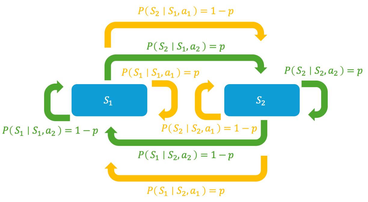
Figure 4: Example Mean Field Game Transition

Appendix G Average-Reward MDP – Detailed Formulation and Algorithm

Consider a standard average-reward MDP characterized by state space ${\cal S}$, action space ${\cal A}$, transition kernel ${\cal P}:{\cal S}\times{\cal A}\rightarrow\Delta_{{\cal S}}$, and reward function $r:{\cal S}\times{\cal A}\rightarrow[0,1]$. The cumulative reward collected by a policy $\pi:{\cal S}\rightarrow\Delta_{{\cal A}}$ is denoted by $J_{\text{MDP}}(\pi)$

$$J_{\text{MDP}}(\pi)\triangleq\mathbb{E}_{a_{k}\sim\pi(\cdot\mid s_{k}),s_{k+1}\sim{\cal P}(\cdot\mid s_{k},a_{k})}[\textstyle\sum_{k=0}^{\infty}r(s_{k},a_{k})\mid s_{0}=s].$$ (171)

The policy optimization objective under softmax parameterization is

$$\max_{\theta}\quad J_{\text{MDP}}(\pi_{\theta}).$$ (172)

The differential value function under policy $\pi_{\theta}$ is

$$V_{\text{MDP}}^{\pi_{\theta}}(s)=\mathbb{E}_{a_{k}\sim\pi_{\theta}(\cdot\mid s_{k}),s_{k+1}\sim{\cal P}(\cdot\mid s_{k},a_{k})}\Big{[}\sum_{k=0}^{\infty}\big{(}r(s_{k},a_{k})-J_{\text{MDP}}(\pi)\big{)}\mid s_{0}=s\Big{]}.$$

We use $P^{\pi}$ and $\nu^{\pi}$ to denote the transition probability matrix and the stationary distribution of states under the control of $\pi$. The policy gradient is

$$\nabla_{\theta}J_{\text{MDP}}(\pi_{\theta})=\mathbb{E}_{s\sim\nu^{\pi_{\theta}},a\sim\pi_{\theta}(\cdot\mid s),s^{\prime}\sim{\cal P}(\cdot\mid s,a,\mu)}\Big{[}(r(s,a)+V_{\text{MDP}}^{\pi_{\theta}}(s^{\prime})-V_{\text{MDP}}^{\pi_{\theta}}(s))\nabla_{\theta}\log\pi_{\theta}(a\mid s)\Big{]},$$ (173)

and $V_{\text{MDP}}^{\pi}$ satisfies the Bellman equation

$$V_{\text{MDP}}^{\pi_{\theta}}=\sum_{a}\pi_{\theta}(a\mid\cdot)r(\cdot,a)+J_{\text{MDP}}(\pi_{\theta}){\mathbf{1}}_{|{\cal S}|}+(P^{\pi_{\theta}})^{\top}V_{\text{MDP}}^{\pi_{\theta}}.$$ (174)

The algorithm for optimizing $J_{\text{MDP}}$ in an average-reward MDP, simplified from Algorithm 1, is presented in Algorithm 2. We have three main iterates in the algorithm, namely, policy parameter $\theta_{k}$ and value function estimates $\hat{V}_{k}$ and $\hat{V}_{k}$ which are used to track $V_{\text{MDP}}^{\pi_{\theta_{k}}}$ and $J_{\text{MDP}}(\pi_{\theta_{k}})$. The policy parameter is updated along the direction of an approximated policy gradient, while the value functions are updated to solve (174) and (172) using stochastic approximation.

Algorithm 2 Online Actor Critic Algorithm for Average-Reward MDP

1:  Initialize: policy parameter $\theta_{0}\in\mathbb{R}^{|{\cal S}|\times|{\cal A}|}$, value function estimate $\hat{V}_{0}\in\mathbb{R}^{|{\cal S}|},\hat{J}_{0}\in\mathbb{R}$, gradient/operator estimates $f_{0}=0\in\mathbb{R}^{|{\cal S}||{\cal A}|},g_{0}^{V}=0\in\mathbb{R}^{|{\cal S}|},g_{0}^{J}=0\in\mathbb{R}$

2:  Sample: initial state $s_{0}\in{\cal S}$ randomly

3:  for iteration $k=0,1,2,...$ do

4:     Take action $a_{k}\sim\pi_{\theta_{k}}(\cdot\mid s_{k})$. Observe reward $r(s_{k},a_{k})$ and next state $s_{k+1}\sim{\cal P}(\cdot\mid s_{k},a_{k})$

5:     Policy (actor) update:

$$\theta_{k+1}=\theta_{k}+\alpha_{k}f_{k}.$$

6:     Value function (critic) update:

$$\hat{V}_{k+1}=\Pi_{B_{V}}(\hat{V}_{k}+\beta_{k}g_{k}^{V}),\quad\hat{J}_{k+1}=\Pi_{[0,1]}(\hat{J}_{k}+\beta_{k}g_{k}^{J}).$$

7:     Gradient/Operator estimate update:

$$f_{k+1} =(1-\lambda_{k})f_{k}+\lambda_{k}(r(s_{k},a_{k})+\hat{V}_{k}(s_{k+1}))\nabla\log\pi_{\theta_{k}}(a_{k}\mid s_{k}),$$

$$g_{k+1}^{V} =(1-\lambda_{k})g_{k}^{V}+\lambda_{k}(r(s_{k},a_{k})-\hat{J}_{k}+\hat{V}_{k}(s_{k+1})-\hat{V}_{k}(s_{k}))e_{s_{k}}$$

$$g_{k+1}^{J} =(1-\lambda_{k})g_{k}^{J}+\lambda_{k}c_{J}(r(s_{k},a_{k})-\hat{J}_{k}).$$

8:  end for

Appendix H Simulation Details

We choose the reward function to be

$$r(s,a,\mu)=\mu(s)+\omega_{r}(s,a)*0.1,\quad\forall s,a,$$

where $\omega_{r}(s,a)\in\mathbb{R}$ is sampled from the standard normal distribution.

The transition kernel ${\cal P}$ is also randomly generated such that for all $s,a$

$${\cal P}(\cdot\mid s,a,\mu)\propto\omega_{P}(s,a)+\mu,$$

where $\omega_{P}(s,a)\in\mathbb{R}^{|{\cal S}|}$ is drawn element-wise i.i.d. from the standard uniform distribution.

For the proposed algorithm algorithm, we select the initial step size parameters to be $\alpha_{0}=10$, $\beta_{0}=0.1$, $\xi_{0}=0.02$, and $\lambda_{0}=1$. The step size parameters for the algorithm in Zaman et al. [2023] are taken from the paper in the Numerical Results section. We tried to adjust the parameters of their algorithm in an attempt to see whether we can get it to converge faster, and found out that the parameters prescribed in the paper are good enough and hard to improve at least locally.

References

- Agarwal et al. [2021] Alekh Agarwal, Sham M Kakade, Jason D Lee, and Gaurav Mahajan. On the theory of policy gradient methods: Optimality, approximation, and distribution shift. Journal of Machine Learning Research, 22(98):1–76, 2021.
- Alasseur et al. [2020] Clémence Alasseur, Imen Ben Taher, and Anis Matoussi. An extended mean field game for storage in smart grids. Journal of Optimization Theory and Applications, 184:644–670, 2020.
- An et al. [2024] Jing An, Jianfeng Lu, Yue Wu, and Yang Xiang. Why does the two-timescale q-learning converge to different mean field solutions? a unified convergence analysis. arXiv preprint arXiv:2404.04357, 2024.
- Anahtarcı et al. [2020] Berkay Anahtarcı, Can Deha Karıksız, and Naci Saldi. Value iteration algorithm for mean-field games. Systems & Control Letters, 143:104744, 2020.
- Anahtarci et al. [2023] Berkay Anahtarci, Can Deha Kariksiz, and Naci Saldi. Q-learning in regularized mean-field games. Dynamic Games and Applications, 13(1):89–117, 2023.
- Angiuli et al. [2022] Andrea Angiuli, Jean-Pierre Fouque, and Mathieu Laurière. Unified reinforcement q-learning for mean field game and control problems. Mathematics of Control, Signals, and Systems, 34(2):217–271, 2022.
- Angiuli et al. [2023] Andrea Angiuli, Jean-Pierre Fouque, Mathieu Laurière, and Mengrui Zhang. Convergence of multi-scale reinforcement q-learning algorithms for mean field game and control problems. arXiv preprint arXiv:2312.06659, 2023.
- Carmona et al. [2019] René Carmona, Mathieu Laurière, and Zongjun Tan. Linear-quadratic mean-field reinforcement learning: convergence of policy gradient methods. arXiv preprint arXiv:1910.04295, 2019.
- Carmona et al. [2021] René Carmona, Kenza Hamidouche, Mathieu Laurière, and Zongjun Tan. Linear-quadratic zero-sum mean-field type games: Optimality conditions and policy optimization. Journal of Dynamics and Games, 8(4):403–443, 2021.
- Chen and Zhao [2024] Xuyang Chen and Lin Zhao. Finite-time analysis of single-timescale actor-critic. Advances in Neural Information Processing Systems, 36, 2024.
- Daskalakis et al. [2009] Constantinos Daskalakis, Paul W Goldberg, and Christos H Papadimitriou. The complexity of computing a nash equilibrium. Communications of the ACM, 52(2):89–97, 2009.
- Dianetti et al. [2024] Jodi Dianetti, Salvatore Federico, Giorgio Ferrari, and Giuseppe Floccari. Multiple equilibria in mean-field game models for large oligopolies with strategic complementarities. arXiv preprint arXiv:2401.17034, 2024.
- Fatkhullin et al. [2023] Ilyas Fatkhullin, Anas Barakat, Anastasia Kireeva, and Niao He. Stochastic policy gradient methods: Improved sample complexity for fisher-non-degenerate policies. In International Conference on Machine Learning, pages 9827–9869. PMLR, 2023.
- Fu et al. [2020] Zuyue Fu, Zhuoran Yang, Yongxin Chen, and Zhaoran Wang. Actor-critic provably finds nash equilibria of linear-quadratic mean-field games. In International Conference on Learning Representations, 2020.
- Ganesh et al. [2024] Swetha Ganesh, Washim Uddin Mondal, and Vaneet Aggarwal. Variance-reduced policy gradient approaches for infinite horizon average reward markov decision processes. arXiv preprint arXiv:2404.02108, 2024.
- Geist et al. [2021] Matthieu Geist, Julien Pérolat, Mathieu Laurière, Romuald Elie, Sarah Perrin, Olivier Bachem, Rémi Munos, and Olivier Pietquin. Concave utility reinforcement learning: The mean-field game viewpoint. arXiv preprint arXiv:2106.03787, 2021.
- Gu et al. [2023] Haotian Gu, Xin Guo, Xiaoli Wei, and Renyuan Xu. Dynamic programming principles for mean-field controls with learning. Operations Research, 71(4):1040–1054, 2023.
- Guo et al. [2019] Xin Guo, Anran Hu, Renyuan Xu, and Junzi Zhang. Learning mean-field games. Advances in neural information processing systems, 32, 2019.
- Guo et al. [2024] Xin Guo, Anran Hu, and Junzi Zhang. Mf-omo: An optimization formulation of mean-field games. SIAM Journal on Control and Optimization, 62(1):243–270, 2024.
- Huang et al. [2006] Minyi Huang, Roland P Malhamé, and Peter E Caines. Large population stochastic dynamic games: closed-loop mckean-vlasov systems and the nash certainty equivalence principle. Communications in Information and Systems, 6(3):221–252, 2006.
- Huang et al. [2007] Minyi Huang, Peter E Caines, and Roland P Malhame. Large-population cost-coupled lqg problems with nonuniform agents: Individual-mass behavior and decentralized -nash equilibria. IEEE transactions on automatic control, 52(9):1560–1571, 2007.
- Jiang et al. [2019] Yanxiang Jiang, Yabai Hu, Mehdi Bennis, Fu-Chun Zheng, and Xiaohu You. A mean field game-based distributed edge caching in fog radio access networks. IEEE Transactions on Communications, 68(3):1567–1580, 2019.
- Kumar et al. [2024] Navdeep Kumar, Yashaswini Murthy, Itai Shufaro, Kfir Y Levy, R Srikant, and Shie Mannor. On the global convergence of policy gradient in average reward markov decision processes. arXiv preprint arXiv:2403.06806, 2024.
- Lasry and Lions [2007] Jean-Michel Lasry and Pierre-Louis Lions. Mean field games. Japanese journal of mathematics, 2(1):229–260, 2007.
- Li et al. [2020] Lixin Li, Qianqian Cheng, Xiao Tang, Tong Bai, Wei Chen, Zhiguo Ding, and Zhu Han. Resource allocation for noma-mec systems in ultra-dense networks: A learning aided mean-field game approach. IEEE Transactions on Wireless Communications, 20(3):1487–1500, 2020.
- Liu et al. [2020] Yanli Liu, Kaiqing Zhang, Tamer Basar, and Wotao Yin. An improved analysis of (variance-reduced) policy gradient and natural policy gradient methods. Advances in Neural Information Processing Systems, 33:7624–7636, 2020.
- Mandal et al. [2023] Debmalya Mandal, Stelios Triantafyllou, and Goran Radanovic. Performative reinforcement learning. In International Conference on Machine Learning, pages 23642–23680. PMLR, 2023.
- Mao et al. [2022] Weichao Mao, Haoran Qiu, Chen Wang, Hubertus Franke, Zbigniew Kalbarczyk, Ravishankar Iyer, and Tamer Basar. A mean-field game approach to cloud resource management with function approximation. Advances in Neural Information Processing Systems, 35:36243–36258, 2022.
- Mei et al. [2020] Jincheng Mei, Chenjun Xiao, Csaba Szepesvari, and Dale Schuurmans. On the global convergence rates of softmax policy gradient methods. In International conference on machine learning, pages 6820–6829. PMLR, 2020.
- Narasimha et al. [2019] Dheeraj Narasimha, Srinivas Shakkottai, and Lei Ying. A mean field game analysis of distributed mac in ultra-dense multichannel wireless networks. In Proceedings of the Twentieth ACM International Symposium on Mobile Ad Hoc Networking and Computing, pages 1–10, 2019.
- Nutz et al. [2020] Marcel Nutz, Jaime San Martin, and Xiaowei Tan. Convergence to the mean field game limit: A case study. The Annals of Applied Probability, 30(1), 2020.
- Olshevsky and Gharesifard [2023] Alex Olshevsky and Bahman Gharesifard. A small gain analysis of single timescale actor critic. SIAM Journal on Control and Optimization, 61(2):980–1007, 2023.
- Panda and Bhatnagar [2024] Prashansa Panda and Shalabh Bhatnagar. Critic-actor for average reward mdps with function approximation: A finite-time analysis. arXiv preprint arXiv:2402.01371, 2024.
- Perolat et al. [2021] Julien Perolat, Sarah Perrin, Romuald Elie, Mathieu Laurière, Georgios Piliouras, Matthieu Geist, Karl Tuyls, and Olivier Pietquin. Scaling up mean field games with online mirror descent. arXiv preprint arXiv:2103.00623, 2021.
- Perrin et al. [2020] Sarah Perrin, Julien Pérolat, Mathieu Laurière, Matthieu Geist, Romuald Elie, and Olivier Pietquin. Fictitious play for mean field games: Continuous time analysis and applications. Advances in neural information processing systems, 33:13199–13213, 2020.
- Saldi et al. [2018] Naci Saldi, Tamer Basar, and Maxim Raginsky. Markov–nash equilibria in mean-field games with discounted cost. SIAM Journal on Control and Optimization, 56(6):4256–4287, 2018.
- Sutton et al. [1999] Richard S Sutton, David McAllester, Satinder Singh, and Yishay Mansour. Policy gradient methods for reinforcement learning with function approximation. Advances in neural information processing systems, 12, 1999.
- Tsitsiklis and Van Roy [1999] John N Tsitsiklis and Benjamin Van Roy. Average cost temporal-difference learning. Automatica, 35(11):1799–1808, 1999.
- Wang [2024] Bing-Chang Wang. Leader–follower mean field lq games: A direct method. Asian Journal of Control, 26(2):617–625, 2024.
- Wu et al. [2020] Yue Frank Wu, Weitong Zhang, Pan Xu, and Quanquan Gu. A finite-time analysis of two time-scale actor-critic methods. Advances in Neural Information Processing Systems, 33:17617–17628, 2020.
- Xie et al. [2021] Qiaomin Xie, Zhuoran Yang, Zhaoran Wang, and Andreea Minca. Learning while playing in mean-field games: Convergence and optimality. In International Conference on Machine Learning, pages 11436–11447. PMLR, 2021.
- Xu et al. [2018] Yang Xu, Lixin Li, Zihe Zhang, Kaiyuan Xue, and Zhu Han. A discrete-time mean field game in multi-uav wireless communication systems. In 2018 IEEE/CIC International Conference on Communications in China (ICCC), pages 714–718. IEEE, 2018.
- Yang et al. [2018] Jiachen Yang, Xiaojing Ye, Rakshit Trivedi, Huan Xu, and Hongyuan Zha. Learning deep mean field games for modeling large population behavior. In International Conference on Learning Representations, 2018.
- Yardim et al. [2023] Batuhan Yardim, Semih Cayci, Matthieu Geist, and Niao He. Policy mirror ascent for efficient and independent learning in mean field games. In International Conference on Machine Learning, pages 39722–39754. PMLR, 2023.
- Yardim et al. [2024] Batuhan Yardim, Artur Goldman, and Niao He. When is mean-field reinforcement learning tractable and relevant? arXiv preprint arXiv:2402.05757, 2024.
- Zaman et al. [2020] Muhammad Aneeq uz Zaman, Kaiqing Zhang, Erik Miehling, and Tamer Bașar. Reinforcement learning in non-stationary discrete-time linear-quadratic mean-field games. In 2020 59th IEEE Conference on Decision and Control (CDC), pages 2278–2284. IEEE, 2020.
- Zaman et al. [2023] Muhammad Aneeq uz Zaman, Alec Koppel, Sujay Bhatt, and Tamer Basar. Oracle-free reinforcement learning in mean-field games along a single sample path. In International Conference on Artificial Intelligence and Statistics, pages 10178–10206. PMLR, 2023.
- Zaman et al. [2024] Muhammad Aneeq uz Zaman, Alec Koppel, Mathieu Laurière, and Tamer Başar. Independent rl for cooperative-competitive agents: A mean-field perspective. arXiv preprint arXiv:2403.11345, 2024.
- Zeng and Doan [2024] Sihan Zeng and Thinh T Doan. Fast two-time-scale stochastic gradient method with applications in reinforcement learning. arXiv preprint arXiv:2405.09660, 2024.
- Zeng et al. [2022] Sihan Zeng, Thinh T Doan, and Justin Romberg. Finite-time complexity of online primal-dual natural actor-critic algorithm for constrained markov decision processes. In 2022 IEEE 61st Conference on Decision and Control (CDC), pages 4028–4033. IEEE, 2022.
- Zeng et al. [2024] Sihan Zeng, Thinh T Doan, and Justin Romberg. A two-time-scale stochastic optimization framework with applications in control and reinforcement learning. SIAM Journal on Optimization, 34(1):946–976, 2024.
- Zhang et al. [2024] Fengzhuo Zhang, Vincent Tan, Zhaoran Wang, and Zhuoran Yang. Learning regularized monotone graphon mean-field games. Advances in Neural Information Processing Systems, 36, 2024.
- Zhang et al. [2021a] Sheng Zhang, Zhe Zhang, and Siva Theja Maguluri. Finite sample analysis of average-reward td learning and -learning. Advances in Neural Information Processing Systems, 34:1230–1242, 2021a.
- Zhang et al. [2021b] Yaoyu Zhang, Jian Sun, and Chenye Wu. Vehicle-to-grid coordination via mean field game. IEEE Control Systems Letters, 6:2084–2089, 2021b.
- Zou et al. [2019] Shaofeng Zou, Tengyu Xu, and Yingbin Liang. Finite-sample analysis for sarsa with linear function approximation. Advances in neural information processing systems, 32, 2019.
Supplementary Materials