Kinks and double-kinks in generalized - and -models
Abstract
Abstract: Examining the and models within a two-dimensional framework in flat spacetime and embracing a theory with unconventional kinetic terms, one investigates the emergence of compactified double kinks/antikinks. We restrict our study to field configurations with minimal energy profiles, i.e., fields with Bogomolnyi-Prasad-Sommerfield (BPS) properties. To accomplish our goal, we adopt non-polynomial functions as generalizing terms, namely, hyperbolic sine and cosine functions. These functions manifest potential minima at in the BPS bound, facilitating the emergence of double-kinks (and double-antikinks). Moreover, as these functions are modified, the double kinks/antikinks may acquire profiles similar to configurations of fields resembling double compactons/anti-compactons.
I Introduction
In the quantum field theory framework, extended objects with conserved topological charges arise due to the continuity of the underlying fields concerning space. These structures are called "kinks" or domain walls. Generally speaking, kinks provide a covariant description of extended particles Finkelstein , Vachaspati . Thus, several works appear in the literature describing kinks in various theories Graham , Zhong , Fabiano . Pioneering studies on kinks belong to Finkelstein Finkelstein , who aimed to provide the properties that a field theory must possess for the existence of kinks and under what circumstances these structures can have spin . Typically, kinks are solitons originating from non-perturbative theories Albayrak . However, these structures emerge as a result of interactions with other particles Albayrak , Rajaraman , Manton , Vilenkin . One highlights that the literature dedicates significant attention to studies on the non-perturbative topological structures and their interactions with perturbative excitations. Besides, one has directed substantial attention towards static and dynamic research of single domain walls. Such emphasis is justified by the challenge posed by any attempt to develop theories, even in the static regime, described by multiple domain walls (i.e., double kinks), while maintaining the preservation of symmetry in flat spacetime. In this study, adopting the two-dimensional spacetime formalism and preserving symmetry, we seek to produce topological structures described by double domain walls (double-kinks) that, in principle, can be compacted.
Interesting models for investigating domain walls arise in higher-order theories. For instance, the models Zhong2 . The interest in these theories stems from the ability of solitons (kinks, double-kinks, or multi-kinks) to experience long-range interactions Belendryasova , Mello , Khare . Within this scenario, the emergence of structures can reveal characteristics of notable relevance. Such a phenomenon arises from the possibility of long-range forces between twists interacting, potentially deforming the topological structures associated with these higher-order configurations Zhong2 . One justifies the interest in obtaining double kink-like structures by their various practical applications. For instance, applications in this field include studies on the emergence of multi-kinks Saadatmand , Marjaneh and collisions involving multi-kinks Gani2 . Motivated by such applications, we describe higher-order theories, such as and models, generalized with BPS properties. We aspire to investigate new classes of solutions that emerge in the BPS bound. For instance, is the emergence of compacted double kinks plausible in this regime? One hopes to elucidate this question throughout the development of this paper.
Striving to accomplish our purpose, we will employ the BPS formalism. This formalism arises in field theory as a convenient tool for solving the equations of motion of static topological fields, allowing the reduction of the order of the Euler-Lagrange equation Bogomolnyi , PS . Concisely, BPS solutions characterize field configurations as energy minima. Although the BPS formalism is particularly useful in describing canonical theories, it is feasible to assume some non-canonical theories and ensure the presence of the BPS property Acalapati . Furthermore, one finds in the literature that models with BPS properties confer stability to the theory of static fields and imply configurations stressless Bazeia0 . Additionally, the BPS formalism has become essential in describing BPS defects with non-canonical kinetic terms FLima1 , FLima2 , Atmaja . Thus, we will adopt the BPS approach to investigate the existence of double domain walls in our theories.
In light of these motivations and adopting the BPS approach, the purpose is to study the emergence of double domain walls (i.e., double kinks) with compact-like features through a kinetically generalized theory. To accomplish this purpose, the and models generalized by non-polynomial functions, specifically hyperbolic functions, will be analyzed. This selection is grounded in the fact that such functions enable the manifestation of potential minima at in the energy saturation bound, allowing the emergence of compacted double-kinks.
We outline our manuscript into three sections. In section II, we discuss the theory of generalized scalar field and impose a constraint on the potential for the generalized dynamics model to admit the BPS property. Furthermore, we subdivide section II into four subsections, demonstrating for the generalized dynamics with hyperbolic functions, the higher-order models ( and ) with symmetry will admit configurations type double-kink compacted. Additionally, one announces our findings in section III.
II The BPS scalar field generalized theory
We start our study by investigating a mechanism that facilitates the production of double-kink structures in a flat two-dimensional theory111We use the metric signature .. Thus, one adopts generalized non-canonical theory with symmetry, described by the action
| (1) |
Analyzing the literature highlights the ability to produce new effects capable of simulating geometric modifications that impact the physical aspects of topological structures through the extension of the theory’s symmetry Bazeia . Generally speaking, to generate the possibility of contracted geometrically structures or deformed kink with the emergence of internal structures, one adopts theories described by the action , namely,
| (2) |
Let us deviate from the usual approach in our work, which considers theories with extended symmetry. Here, we adopt the action (1). In this scenario, will be a generalizing function, and potential. Consequently, upon adopting the action (1), one obtains
| (3) |
In this scenario, denotes the real scalar field. Furthermore, one defines and .
Let us now proceed to particularize the theory for the static case, i.e., adopting , where denotes the position. This consideration enables us to express the equation of motion as
| (4) |
In the static regime, the -field energy is
| (5) |
Allow us to rearrange the field energy as
| (6) |
The function is designated as an auxiliary function or superpotential. The implementation of the function is essential once it establishes a correspondence between , the potential, and the energy through an appropriate choice of Vachaspati . Thereby, let us assume that the superpotential relates to the potential through a constraint
| (7) |
Note that the -field energy will be
| (8) |
One defines the BPS energy as
| (9) |
Hence, the full energy is
| (10) |
Therefore, one can inferred that . Thus, at the energy bound, i.e., , the self-dual equation is
| (11) |
In this regime, the BPS energy density will be
| (12) |
II.1 The BPS theory for the symmetric and models
At this juncture, it needs to select a superpotential profile to ensure the existence of the BPS property. In our context, we will adopt two distinct superpotentials, i.e.,
| (13) |
and
| (14) |
Considering Eq. (7), the BPS potentials will be the generalized potentials and described, respectively, as
| (15) |
and
| (16) |
These potentials are remarkable as they enable the geometric contraction on the topological structures Lima , Bazeia . A theory [Eq. (15)] has been utilized to derive compact-like vortex configurations Lima . Furthermore, the theory [Eq. (16)] has proven effective in compactifying structures of the real scalar field Bazeia . Besides, some researchers adopt a few high-order theories responsible for describing kinks. For instance, Demirkaya et al. Demirkaya investigates the dynamics of kinks in a system. Additionally, Gani et al. Gani analyzes the interaction of kinks in a theory. However, all results from these theories yield kink-like configurations or multi-kinks interpolating between two topological sectors. In contrast to the literature, we aim to obtain configurations of genuine double-kinks, which may exhibit a compacted profile. To accomplish this purpose, we will assume three generalized functions, i.e.,
| (17) |
Now, we will focus on the study of cases (17) involving the BPS potentials (15) and (16).
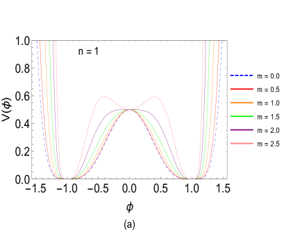
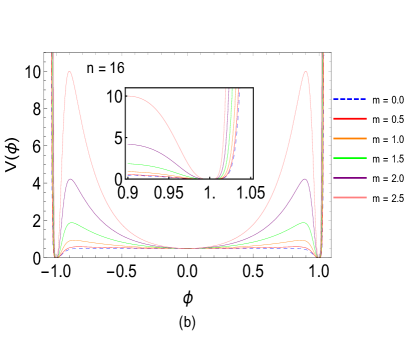
II.1.1 The symmetric model: the case
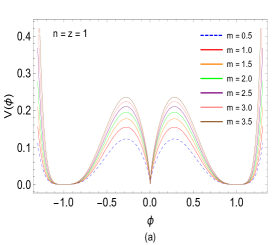
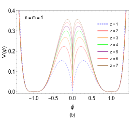
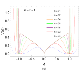
For the symmetric model with the generalizing function , one obtains the BPS potential
| (18) |
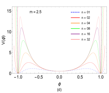
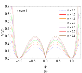
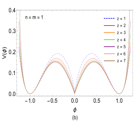
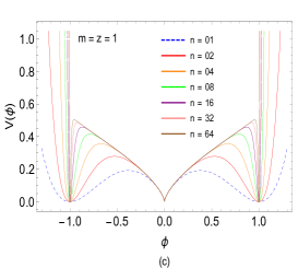
We display the behavior of the potential (18) in Figs. 1(a), 1(b), 1(c), and 1(d). Potentials with similar characteristics (however ) emerge in Ref. Gani when investigating kinks collisions with opposite topological charges. Here, we will show that one can obtain true double-kinks and compactify them for the BPS theory with potential (18).

Considering the superpotential (12), one arrives at the self-dual equation
| (19) |
In this scenario, the parameter adjusts the dimension of the theory, and () represents the potential minimum. Here, , and .
To ensure the existence of a kink-like scalar field kink-like (and antikink-like), one must respect the topological boundary condition, i.e.,
| (20) |
and
| (21) |
Adopting the topological boundary (20) and (21), one obtains the BPS energy, namely,
| (22) |
where and the BPS energy density is
| (23) |
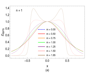
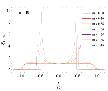
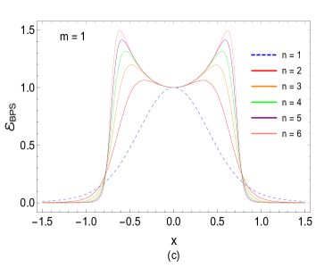
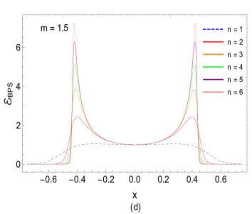
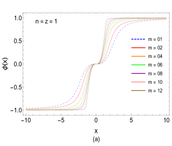
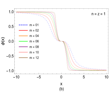
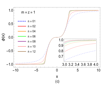
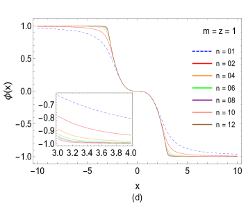
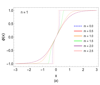
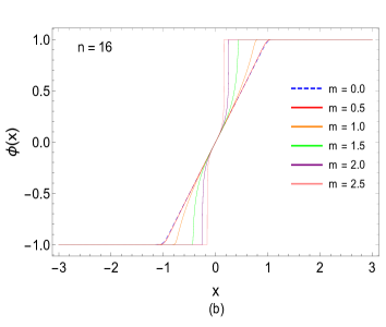
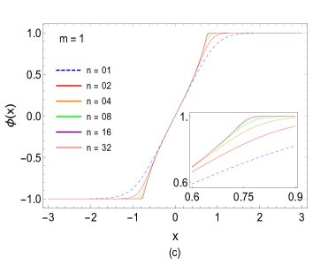
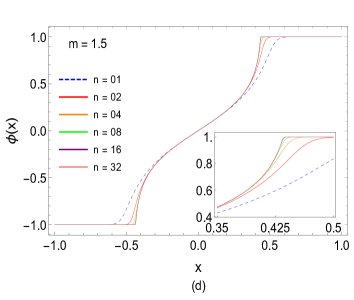
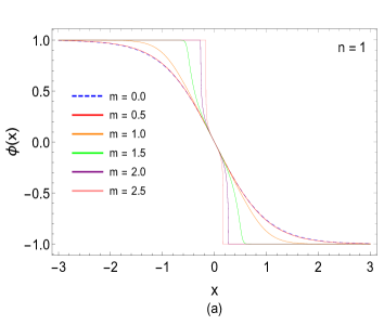
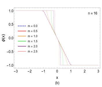
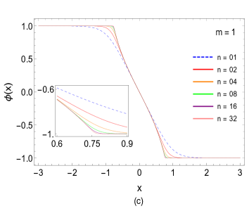
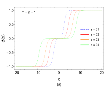
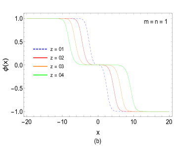
Let us now proceed to investigate the solution of the self-dual equations of the system. For this purpose, we will discretize the equation by considering the domain of the independent variable at points. For instance, ; subsequently, we will employ the interpolation method to estimate the solution of the scalar field, considering the intermediate points Hildebrand . Adopting this methodology, the numerical solutions of equation (19) are obtained. Please see Figs. 2[(a)-(d)] and 3[(a)-(d)] for double-kink and double-antikink configurations, respectively. For the sake of simplicity, one assumes . This choice does not entail loss and facilitates our analysis once these parameters only adjust the field amplitudes.
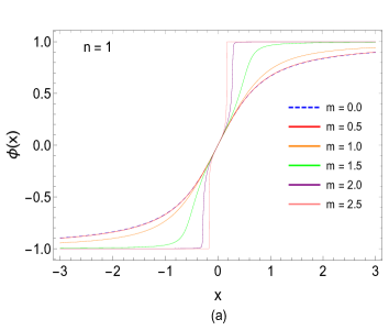
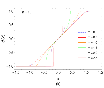
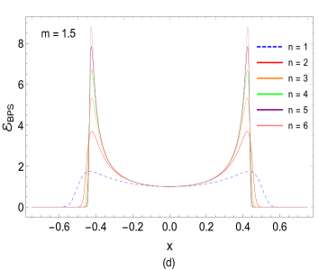
Considering the numerical solutions presented in Figs. 2 and 3, the BPS energy density is numerically obtained. We expose the BPS energy density in terms of the position in Figs. 4[(a)-(d)]. One notes that the scalar field deforms into structures resembling the double kinks. Besides, we note the emergence of new critical energy points in the BPS energy density confirms this profile. Additionally, for appropriate variations for keeping fixed, double-kink-like configurations emerge, yielding compact-like field configurations. That behavior must be the potential minima, become extremely localized, resulting in a scalar field compactification.
II.1.2 The symmetric model: the case
Considering the generalizing function and the superpotential (13), the BPS potential is
| (24) |
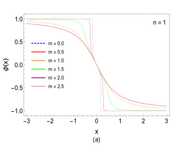
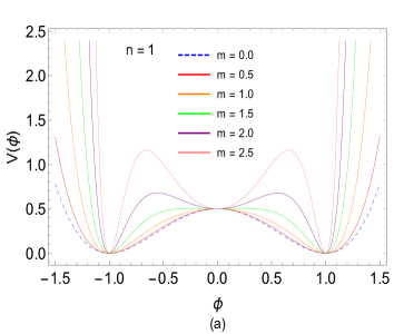
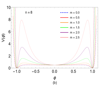
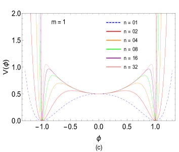
We are motivated to investigate this second model, characterized by the generalizing function , due to its ability to produce a potential minimum at . The emergence of potential minimum suggests the possibility of deformation of the topological structures, resulting in the formation of double kinks. In Figs. 5[(a)-(c)], one exposes the potential corresponding to this model with the generalizing function .
In this scenario, the BPS equation is
| (25) |
where . Furthermore, we retrieve the generalized model. One can note that , one has the theory interpolating between the vacua .
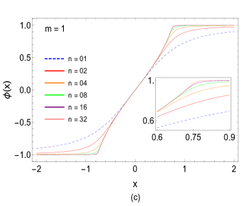
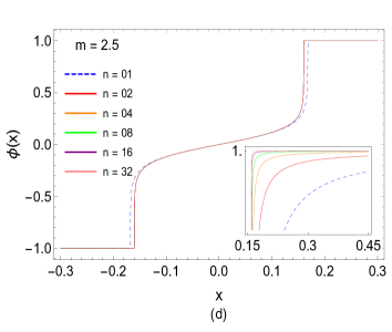
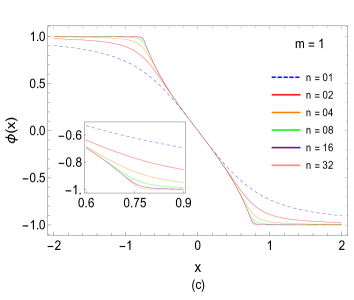
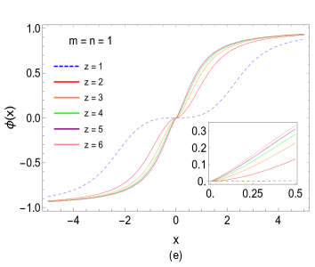
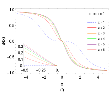
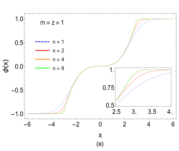
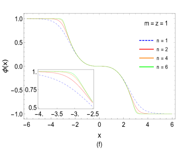
Investigating the numerical field solutions, we discretize the domain of the variable of Eq. (25), as mentioned previously. The numerical interpolation allows us to estimate the numerical solution of Eq. (25) Hildebrand . Through this approach, one obtains the numerical solutions displayed in Figs. 6[(a)-(f)].
Note that
| (26) |
Thereby, when , the self-dual equation is
| (27) |
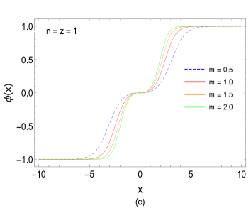
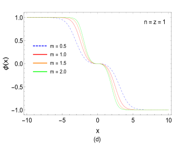
which leads us to kink-like solutions, see Fig. 6(f), when the parameter increases. So, one concludes that varying the -parameter transforms kink-like solutions into double-kinks. Moreover, varying the and parameters compactifies the field solutions, rendering them type to double-compacton solutions.
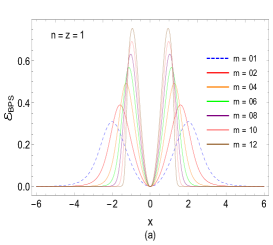
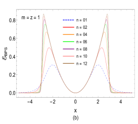
Naturally, the BPS energy density of these field profiles is
| (28) |
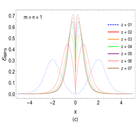
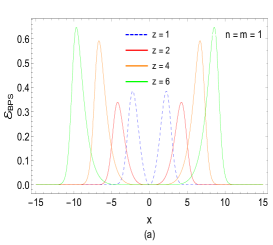
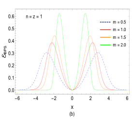
Considering the numerical solutions presented in Fig. 6 and utilizing Eq. (28), the BPS energy density of the fields is numerically obtained, as shown in Figs. 7[(a)-(c)]. It is notable from the analysis of the BPS energy density profiles the existence of solutions resembling double-kinks varying the parameters , , and . This confirmation is due to the energy profile splitting into two symmetric parts around . Naturally, by increasing the parameter , the energy regions become more localized. Meanwhile, as the parameter varies, the asymptotic behavior of the BPS energy density tends to zero rapidly, suggesting the existence of compacted double-kink solutions. Finally, increasing the parameter, i.e., , the BPS energy density becomes similar to kink-like configurations. One can note more details of these results in Figs. 7[(a)-(c)].
II.1.3 The symmetric model: the case
For the theory [Eq. (16)] with generalizing function , one arrives at the BPS potential
| (29) |
We display the potentials (29) in Fig. 8[(a)-(d)]. Note that, owing to the generalized BPS potential contribution being -like with a profile less localized, the scalar field exhibits behavior comparable to . Thereby, the field will suffer smoother deformation. Therefore, one concludes that the scalar field profiles resemble the double-kinks and compactons of the generalized theory.
In this case, the BPS equation is
| (30) |
Using again the numerical interpolation approach (please refer to the preceding subsections), one obtains the numerical solutions of the scalar field. We present these solutions in Figs. (9).
These field configurations carry a BPS energy, i.e.,
| (31) |
Thus, the BPS energy density will be
| (32) |
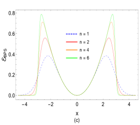
Therefore, adopting Eq. (32) and considering the numerical solutions exposed in Figs. 9 and 10, one obtains the BPS energy density. We display the BPS energy density in Fig. 11, where one notes that the energy suggests the emergence of compacted double-kink structures.
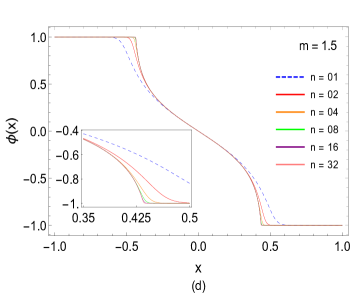
II.1.4 The symmetric model: the case
Now, let us analyze the final case, i.e., adopting a generalizing function in the theory. In this case, the BPS potential is
| (33) |
We present the BPS potential of the scalar field in Fig. 12[(a)-(c)]. In this case, one notes that in the case of the hyperbolic sine generalizing function, we again have the existence of vacua . However, varying , the amplitude of the potential barrier around becomes more pronounced, allowing the emergence of a double kink matter field. Meantime, the parameter adjusts the position of the potential minima. Lastly, varying locates the potential minima at , enabling the emergence of solutions with compacton-like profiles. For further details, see Fig. 12.
In this case, the BPS equation is
| (34) |
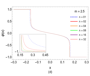
Using the numerical interpolation approach investigates the numerical solutions of the scalar field. The numerical results of the scalar field are depicted in Fig. 13[(a)-(f)]. In this case, one notes that all profiles of the scalar field exhibit double-kink-like behavior with variations of the parameters; for instance, varying the parameter produces compacted double-kink-like structures.
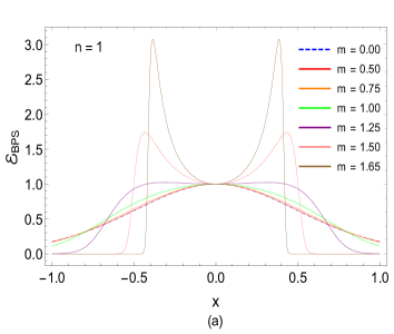
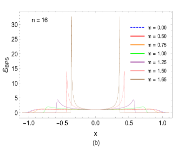
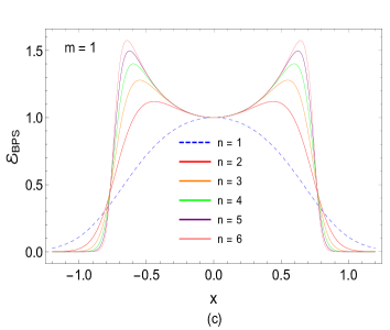
Furthermore, it is necessary to highlight that these configurations possess the BPS energy as announced in Eq. (31), and their BPS energy density will be
| (35) |
Considering the numerical solutions exposed in Fig. 13 together with Eq. (35), one obtains the numerical solutions of the BPS energy densities of the compacted double-kinks. Naturally, these results are due to the generalization profile adopted. We announce more details about the physical implications in the final remarks.
III Final remarks
Throughout this work, we examined the and theory within a flat space-time framework. By adopting non-canonical contributions from the kinetic term, i.e., , one noted that non-canonical theories admit classes of solutions resembling double-kink-like (and double-antikink-like). Furthermore, one observed that with appropriate adjustments to the profile of the generalizing function, we can compact these configurations comparable to double-kinks (double-antikinks).
The theories and adopted were, respectively, described by the interactions
| (36) |
In this scenario, the generalizing functions are: , , and . We adopted these choices because they allow the emergence of energy minima at on the BPS bound. Thereby, the minimal energy configurations geometrically deformed arise, announcing new classes of scalar field solutions.
One highlights that the chosen theoretical models are suitable also due to their asymptotic behavior. For instance, considering the generalizing function , we reached the usual theories and as . The usual theory is reobtained in the case as . However, in the case as , one obtains a polynomial-like generalizing theory, i.e., (adopting ) described by well-defined double domain walls, see Figs. 13[(a) and (b)]. Lastly, it is worth highlighting that in all cases, when one of the potential minima becomes more localized, the process of compactification of the scalar field solutions occurs. To conclude, we announced in our work, using cases with unusual kinematics, how to obtain double domain walls smoothly (and abruptly) and their compactification.
IV Acknowledgment
The authors express their gratitude to FAPEMA and CNPq (Brazilian research agencies) for their invaluable financial support. F. C. E. L. is supported by FAPEMA BPD-05892/23. R. C. acknowledges the support from the grants CNPq/312155/2023-9, FAPEMA/UNIVERSAL-00812/19, and FAPEMA/APP-12299/22. C. A. S. A. is supported by CNPq 309553/2021-0 (CNPq/Produtividade) and project 200387/2023-5. Furthermore, C. A. S. A. acknowledges the Department of Theoretical Physics & IFIC from the University of Valencia for their warm hospitality.
References
- [1] D. Finkelstein, J. Math. Phys. 7 (1966) 1218.
- [2] T. Vachaspati, Kinks and Domain Walls: An Introduction to Classical and Quantum Solitons, (Cambridge University Press, Cambridge, England) 2006.
- [3] N. Graham and H. Weigel, Phys. Lett. B 852 (2024) 138638.
- [4] Y. Zhong, H. Guo and Y. -X. Liu, Phys. Lett. B 849 (2024) 138471.
- [5] F. F. Santos and F. A. Brito, Phys. Lett. B 850 (2024) 138543.
- [6] O. Albayrak and T. Vachaspati, Phys. Rev. D 109 (2024) 036001.
- [7] R. Rajaraman, Solitons and Instantons. An Introduction to Solitons and Instantons in Quantum Field Theory (North-Holland, Amsterdam, 1982).
- [8] N. S. Manton and P. Sutcliffe, Topological Solitons, Cambridge Monographs on Mathematical Physics (Cambridge University Press, Cambridge, England, 2004).
- [9] A. Vilenkin and E. P. S. Shellard, Cosmic Strings and Other Topological Defects (Cambridge University Press, Cambridge, England, 2000).
- [10] Y. Zhong, X. -L. Du, Z. -C. Jiang, Y. -X. Liu and Y. -Q. Wang, JHEP 02 (2020) 153.
- [11] E. Belendryasova and V.A. Gani, Commun. Nonlinear Sci. Numer. Simul. 67 (2019) 414.
- [12] B. A. Mello, J. A. Gonzalez, L. E. Guerrero and E. Lopez-Atencio, Phys. Lett. A 244 (1998) 277.
- [13] A. Khare, I. C. Christov and A. Saxena, Phys. Rev. E 90 (2014) 023208.
- [14] D. Saadatmand, S. V. Dmitriev and P. G. Kevrekidis, Phys. Rev. D 92 (2015) 056005.
- [15] A. M. Marjaneh, D. Saadatmand, K. Zhou, S.V. Dmitriev and M. E. Zomorrodian, Commun. Nonlinear Sci. Numer. Simul. 49 (2017) 30.
- [16] V. A. Gani, A. M. Marjaneh and D. Saadatmand, Eur. Phys. J. C 79 (2019) 620.
- [17] E. B. Bogomolny, Sov. J. Nucl. Phys. 24 (1976) 449.
- [18] M. K. Prasad and C. M. Sommerfield, Phys. Rev. Lett. 35 (1975) 760.
- [19] E. Acalapati and H. S. Ramadhan, Ann. Phys. 465 (2024) 169665.
- [20] D. Bazeia, L. Losano and R. Menezes, Phys. Lett. B 668 (2008) 246.
- [21] F. C. E. Lima, A. Y. Petrov and C. A. S. Almeida, Phys. Rev. D 103 (2021) 096019.
- [22] F. C. E. Lima, A. Y. Petrov and C. A. S. Almeida, Phys. Rev. D 105 (2022) 056005.
- [23] A. N. Atmaja, Phys. Lett. B 768 (2017) 351.
- [24] D. Bazeia, M. A. Liao and M. A. Marques, Eur. Phys. J. Plus 135 (2020) 383.
- [25] F. C. E. Lima and C. A. S. Almeida, Ann. Phys. 434 (2021) 168648.
- [26] A. Demirkaya, R. Decker, P. G. Kevrekidis, I. C. Christov and A. Saxena, JHEP 12 (2017) 071.
- [27] V. Gani, A. M. Marjaneh and K. Javidan, Eur. Phys. J. C 81 (2021) 1124.
- [28] F. B. Hildebrand, Introduction to Numerical Analysis, (Dover Publications, Inc., 2nd ed., New York, 1956)