Kolmogorov turbulence in atomic Bose-Einstein condensates

Abstract

We investigated turbulence in atomic Bose-Einstein condensates (BECs) using a minimally destructive, impurity injection technique analogous to particle image velocimetry in conventional fluids. Our approach transfers small regions of the BEC into a different hyperfine state, and tracks their displacement ultimately yielding the velocity field. This allows us to quantify turbulence in the same way as conventional in fluid dynamics in terms of velocity-velocity correlation functions called velocity structure functions that obey a Kolmogorov scaling law. Furthermore the velocity increments show a clear fat-tail non-Gaussian distribution that results from intermittency corrections to the initial “K41” Kolmogorov theory. Our observations are fully consistent with the later “KO62” description. These results are validated by a 2D dissipative Gross-Pitaevskii simulation.

Turbulence is a fundamental phenomenon encountered in a wide range of fluids at all scales: from classical systems such as oceans and atmospheres Gargett (1989); Wyngaard (1992); confined and solar plasmas Zhou et al. (2004); Loureiro and Boldyrev (2017); and the self-gravitating media of the large-scale universe Shandarin and Zeldovich (1989) to quantum fluids such as neutron stars Greenstein (1970), superfluid ⁴He  Vinen and Niemela (2002) and atomic Bose-Einstein condensates (BECs)  Henn et al. (2009); Navon et al. (2016). In all of these cases, turbulence is characterized by complex patterns of fluid motion spanning a wide range of length scales. While the understanding of classical turbulence has matured in the past century Sreenivasan (1999), that of quantum systems has many open questions Madeira et al. (2020). For example, in BECs, does there exist a range of length scales—the inertial scale—in which kinetic energy cascades from large to small scale in accordance with a Kolmogorov scaling law? Although this scaling was predicted only for incompressible fluids it has been observed in virtually all turbulent fluids Sreenivasan (1999). Kolmogorov scaling is generally quantified in terms of velocity structure functions (VSFs) that require knowledge of the fluid’s velocity field, which is difficult to measure in quantum gas experiments. In this work we: present a particle imaging velocimetry (PIV) technique Taylor (1938); Adrian and Yao (1985) employing spinor impurities as tracer particles; obtain VSFs in turbulent atomic BECs; and observe Kolmogorov scaling.

Existing experimental evidence for turbulence in atomic BECs relies on time of flight (TOF) measurements are either dominated by interaction driven expansion Henn et al. (2009), or yield momentum distributions Thompson et al. (2013); Navon et al. (2016). Such observations have no clear connection to the VSFs $S_{p}(l)$ which describe various order-$p$ moments of the distribution of velocity increments

$$\delta{\bf v}(\mathbf{x},{\bf l}) =\mathbf{v}(\mathbf{x}+\mathbf{l})-\mathbf{v}(\mathbf{x})$$ (1)

as a function of displacement ${\bf l}$. Without access to VSFs, turbulence in atomic gases lacks a direct point of comparison to other fluids.

Unlike classical fluid flow, superfluid flow is strictly irrotational with a velocity field governed by the phase of the superfluid order parameter $\phi$ via ${\bf v}=\hbar{\bm{\nabla}}\phi/m$. Despite this, it is generally believed that superfluid turbulence obeys the same $S_{p}(l)\propto l^{(p/3)}$ scaling as classical fluids, described by the initial K41 Kolmogorov theory Kolmogorov (1991a, 1941, b); in the case of ${}^{4}\mathrm{He}$ this has been experimentally verified Nore et al. (1997); Stalp et al. (1999) for $p\leq 3$. The more complete KO62 theory Kolmogorov (1962); Obukhov (1962) adds an intermittency correction that becomes important for large $p$ and also predicts that the ensemble probability density function of velocity increments (PDF) is non-Gaussian, with “fat-tails.” Power-law scaling behavior and energy cascade have been observed in the momentum distribution of homogeneously trapped BECs undergoing relaxation Navon et al. (2016); the observed exponent departed from the $-5/3$ prediction of K41 theory for energy cascade [related to the Fourier transform of the $S_{2}(l)$ structure function], and was instead accurately interpreted using a wave turbulence model.

Our cold-atom PIV technique allows us to directly measure the velocity field and thereby both $S_{p}(l)$ and the underlying PDF. As illustrated in Fig. 1(a), we prepare an initial velocity distribution, then create localized “tracer particles” consisting of atoms in a different hyperfine state using a spatially-resolved technique, and, after a $\Delta t$ delay, measure the tracers’ displacement. This then directly leads to the local fluid velocity.

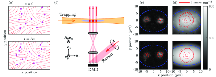
Figure 1: Concept. (a) Top: representative velocity field with tracer particles (bright pink). Bottom: at $t=\Delta t$, tracer particles move from their initial position (dark pink). (b) Schematic of spatially-resolved Raman apparatus used to create tracers. (c) PTAI imaged tracers before (top) and after (bottom) evolution, with initial and final positions shown by crosses and circles respectively. Red circles mark the $1$-$\sigma$ widths of the tracers. (d) Velocity fields in a rotating harmonic trap (red arrows) along with atomic density in grey-scale with blue ellipses placed at $0.75\times$ of the Thomas-Fermi radius. Top and bottom panels display experimental data and GPE simulations respectively.

Experimental method—We used ${}^{87}\mathrm{Rb}$ BECs with $N\approx 2\times 10^{5}$ atoms in the $\ket{F=1,m_{F}=1}$ hyperfine ground state with strong vertical confinement [trap frequency $\omega_{z}/(2\pi)=220\ \mathrm{Hz}$] provided by a $1064\ \mathrm{nm}$ laser with an elliptical cross-section, traveling along $\mathbf{e}_{x}$. Additionally, a digital micromirror device (DMD) patterned a $638\ \mathrm{nm}$ multimode laser traveling along $-\mathbf{e}_{z}$ to provide dynamical ($\approx 3\ {\rm kHz}$ update rate) in-plane potentials $V({\bf r},t)$. An $\approx 0.14\ {\rm mT}$ bias magnetic along $\mathbf{e}_{y}$ created a $\Delta f=1\ \mathrm{MHz}$ Zeeman splitting between consecutive $m_{F}$ states.

Figure 1(b) schematically shows the spatially-resolved Raman setup used to create localized tracer particles. A circularly polarized bichromatic $\approx 790\ \mathrm{nm}$ laser beam traveling along $\mathbf{e}_{z}$ with frequencies spaced by $\Delta f$ drove $m_{F}$-changing Raman transitions with a $50\ \mathrm{kHz}$ Rabi frequency. The beam was patterned by a second DMD, enabling the placement of arbitrary patterns of tracer atoms in $\ket{F=1,m_{F}=0}$. Tracer atoms were selectively measured using partial transfer absorption imaging (PTAI), in which $\approx 6.8\ \mathrm{GHz}$ microwaves transferred the tracers to $\ket{F=2,m_{F}=0}$ where they were detected using resonant absorption imaging. Our imaging system had a nominal $1\ \mu{\rm m}$ resolution, allowing us create and then detect tracers with $1/e$ radius down to $1.6\ \mu{\rm m}$.

In our experimental sequence we first initialized the velocity field of interest and then created a set of $N$ tracers, at positions $\mathbf{r}^{j}_{0}$ in the $\mathbf{e}_{x}$-$\mathbf{e}_{y}$ plane using an $\approx\pi/2$ Raman pulse, with $j=1\ldots N$ [these positions were directly verified by PTAI measurement, as shown for $N=2$ in Fig. 1(c-top)]. After a $\Delta t$ evolution time, we imaged the tracers to obtain the final positions $\mathbf{r}^{j}$ [Fig. 1(c-bottom)]. The velocity at each $\mathbf{r}_{0}^{j}$ was taken as the first order finite-difference ${\bf v}^{j}=(\mathbf{r}^{j}-\mathbf{r}_{0}^{j})/\Delta t$.

Validation in a rotating BEC— Before applying PIV to turbulent systems, we validated the method with harmonically trapped BECs rotating with angular frequency $\Omega$ about $\mathbf{e}_{z}$. The confining DMD generated a rotating in-plane harmonic potential with $(\omega_{x},\omega_{y})=2\pi\times(40,50)\ \mathrm{Hz}$. For slowly rotating systems, such that no vortices are present, the superfluid velocity is expected to exhibit an irrotational pattern $\mathbf{v}=a(y\mathbf{e}_{x}+x\mathbf{e}_{y})$ with $a\propto\Omega$ for small $\Omega$ Pitaevsiii and Stringari (2003). At higher rotation frequencies, when $\Omega$ becomes comparable to the trap frequencies $\omega_{x,y}$, this becomes a metastable configuration with a range of possible instability conditions, the details of which must be obtained numerically Recati et al. (2001); Sinha and Castin (2001). In our case these conditions would limit the rotation frequency to $\Omega\lesssim 2\pi\times 40\ {\rm Hz}$, leading to typical speeds $|{\bf v}|\lesssim 0.25\ \mathrm{mm/s}$. To obtain increased signal, we focused on overcritical systems with $\Omega=2\pi\times 50\ {\rm Hz}$, for which $|\mathbf{v}|\approx 0.7\ \mathrm{mm/s}$.

Experimentally we began with static systems, then linearly increased the angular frequency from zero to $\Omega$ in $15\ \mathrm{ms}$, held $\Omega$ constant for $2\ \mathrm{ms}$ (at which time the BEC rotated by an angle $\theta=\pi/2$) and then performed PIV. In this demonstration we sampled the velocity field on three concentric circles (with radii of $1\ \mathrm{\mu m}$, $2.5\ \mathrm{\mu m}$, and $5\ \mathrm{\mu m}$) with an angular resolution of $\pi/12$, and used an evolution time $\Delta t=1.5\ \mathrm{ms}$. To increase the signal we used tracers with a $2.2\ \mathrm{\mu m}$ diameter and for the smallest circle the tracer size limited the number of tracers to $N=1$, otherwise we used $N=2$. Figure 1(d-top) shows both the atomic density (grey scale) and associated velocity field (red) with the irrotational quadrupole pattern clearly visible. The data is in good agreement with our Gross-Piteavskii equation (GPE) simulations in Fig. 1(d-bottom). This validation of our PIV method also marks the first direct visualization of the irrotational flow pattern in a rotating atomic superfluid .

Structure function—Because Kolmogorov theory is valid for isotropic homogeneous systems, we turned our attention to near-ground state BECs with uniform atomic density. We employed the confining DMD to create a time-independent 2D disk-shaped potential $V({\bf r})=V_{\rm tr}\Theta(|{\bf r}|-r_{\rm tr})$ with radius $r_{\rm tr}=22\ \mathrm{\mu m}$ and depth $V_{\rm tr}\gg\mu$, where $\mu\approx h\times 550\ {\rm Hz}$ is the BEC’s chemical potential .

We then initialized turbulence with a pair of counter-rotating stirring “rods” with $3.5\ \mathrm{\mu m}$ radii (also created by the confining DMD) that locally depleted the atomic density. As shown in Fig. 2(a), the initially overlapping rods followed nominally circular trajectories (red curves, with a $25\ \mathrm{Hz}$ rotational frequency), the radius of which changed every $400\ \mu{\rm s}$ to a random value in the interval $[12\ \mathrm{\mu m},15\ \mathrm{\mu m}]$. The stirring potential was applied for $16\ \mathrm{ms}$; the system was then allowed to relax for $40\ \mathrm{ms}$ prior to PIV measurement (with $\Delta t=0.3\,\mathrm{ms}$ evolution time).

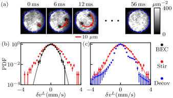
Figure 2: Turbulence. (a) Atomic density measured during the excitation process. The blue circle marks the edge of the trap and red arcs indicate the average path of the stirring rods. (b,c) Histograms of $\delta v^{L}(l=10.6\ \mu m)$ with peak value scaled to $1$ and error bars derived from standard counting uncertainty. (b) Raw data for initial BEC (black, along with Gaussian fit) and with stirring (red). (c) Deconvolved data (blue) and raw data (red, along with a recolvolved curve).

We used tracer patterns consisting of $N=4$ tracers arrayed in a square with three different side-lengths: $10.6\,\mathrm{\mu m}$, $11.4\,\mathrm{\mu m}$, and $12.6\,\mathrm{\mu m}$. Together these patterns gave access to six tracer separations $l$ comprising the side as well as the diagonal lengths. The measured tracer positions $\mathbf{r}^{j}$ were then identified by the center of mass $\overline{\rho^{j}\mathbf{r}}/\overline{\rho^{j}}$ of the transferred atoms. To first order in $\Delta t$ the resulting velocity is the density-weighted (i.e., Favre-averaged Favre (1965)) velocity $\widetilde{\mathbf{v}}=\overline{\rho\mathbf{v}}/\overline{\rho}$, used when applying Kolmogorov theory to compressible fluids Aluie (2011, 2013); Wang et al. (2012) (we omit the tilde in what follows). Each measurement yielded 12 velocity increments $\delta{\bf v}(\mathbf{r}^{j},{\bf l}^{ij})$, with ${\bf r}^{j}$ associated with each tracer and the difference vector ${\bf l}^{ij}=\mathbf{r}_{0}^{i}-\mathbf{r}_{0}^{j}$ to each of the remaining tracers. Figure 2(b) displays the resulting longitudinal PDFs both with (red symbols) and without (black symbols) stirring, ${\rm PDF}_{\rm s}(\Delta v^{L})$ and ${\rm PDF}_{\rm ns}(\Delta v^{L})$ respectively. A ground state BEC’s PDF should resemble a Kronecker-$\delta$ function centered at $0$; here the observed non-zero width $\sigma=0.55(1)\ \mathrm{mm/s}$ provides a measure of the instrumental noise and is well described by a Gaussian (black curve). Although the distribution with stirring (red) is broadened and acquires a “fat tail,” any VSFs computed directly from these data will be significantly contaminated by instrumental noise.

We therefore employed quadratic programming based deconvolution Yang et al. (2020) to approximate the underlying ${\rm PDF_{0}}(\Delta v)$ from raw data [Fig. 2(c)]. This process minimizes the L2 distance $|{\rm PDF}_{\rm s}(\Delta v)-({\rm PDF}_{\rm ns}*{\rm PDF}_{0})(\Delta v)|^{2}$ between the measured distribution and the convolution (denoted by $*$) of the reconstruction with the instrument noise distribution, subject to the constraints that ${\rm PDF_{0}}(\Delta v)$ is: normalized, non-negative, and contains a single maximum. Because “fancy” analysis procedures may introduce unknown artifacts, in what follows we present data derived from the PDF both with and without deconvolution.

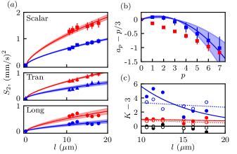
Figure 3: In all panels red and blue denote stirred data with and without deconvolution, respectively, while black indicates unstirred data. (a) Measured $S_{2}(l)$. Each point results the the average of 44 experimental runs, and each run derived $S_{2}(l)$ from about 50 nominally identical experimental repetitions. The uncertainties are the $2$-$\sigma$ standard error of the mean for the set of 44 runs. As described in the text, the curves are fits to the data plotted along with their $2$-$\sigma$ uncertainty band. (b) Intermittency correction with error bars indicating $2$-$\sigma$ uncertainties. The blue curve represents a fit to the KO62 model, with $2$-$\sigma$ confidence band. (c) Excess Kurtosis of transverse (solid) and longitudinal (empty) distributions data each fit to a decaying exponential.

Using PDFs such as these, we obtained the longitudinal $S^{L}_{p}(l)=\langle|\delta{\bf v}(\mathbf{x},{\bf l})\cdot{\bf e}_{l}|^{p}\rangle$, transverse $S^{T}_{p}(l)=\langle|\delta{\bf v}(\mathbf{x},{\bf l})\cdot{\bf e}_{\perp}|^{p}\rangle$, and scalar $S^{S}_{p}(l)=\langle|\delta{\bf v}(\mathbf{x},{\bf l})|^{p}\rangle$ VSFs  . All three 2nd order VSFs derived from this procedure are shown in Fig. 3(a) with and without deconvolution. The primary impact of deconvolution on these data is to reduce the amplitude of the VSFs, as would be expected from the PDF’s reduced width. In both cases the data are compatible with the $S_{2}(l)=s_{2}l^{2/3}$ power-law expected in the K41 assumption, with fits shown by the solid curves (coefficients shown in Table 1). In general, transverse VSFs are expected to be larger than their longitudinal counterparts; for homogenous and isotropic turbulence the second order structure functions have the exact relation $S^{T}_{2}(l)/S^{L}_{2}(l)=4/3$, and indeed we find $s_{2}^{T}/s_{2}^{L}=1.6(1)$ with deconvolution and $1.33(4)$ without.

	$s_{2}^{L}$	$s_{2}^{T}$	$s_{2}^{S}$	$\chi$
		$\times 10^{-3}\ \mathrm{m^{4/3}/s^{2}}$
Expt. Raw	1.06(7)	1.41(2)	2.47(6)	N.A.
Expt. Deconv.	0.52(4)	0.83(4)	1.34(2)	0.04(1)
Numerics	0.329(1)	0.401(2)	0.730(3)	0.023(1)

Table 1: Fit parameters.

Intermittency—Intermittency in turbulence can be be quantified by corrections to K41’s $l^{(p/3)}$ scaling law. We directly obtain scaling exponents $a_{p}$ from power-law fits to the measured $p$-order scalar VSFs; the resulting differences $\varepsilon_{p}=a_{p}-p/3$ are plotted in Fig. 3(b) for stirred data with and without deconvolution (blue and red squares respectively). All three cases show a deviation from $p/3$ scaling that grows with increasing $p$. In detail, the deconvolved data is consistent with the $\varepsilon_{p}=-\chi p(p-3)$ prediction of KO62 theory (solid curve), with a system specific intermittency coefficient $\chi$ obtained by fitting the deconvolved data in Table 1.

The deviation from K41 predictions indicates scale-dependent non-Gaussian behavior in the PDFs. Two widely separated tracers should have uncorrelated motion, resulting in Gaussian PDFs for the velocity increments. However, if correlations develop with decreasing tracer separation, the resulting PDFs can become non-Gaussian as we observe in Fig. 2(b-c). We describe the non-Gaussian behavior of these distributions in terms of the kurtosis $K$, which quantifies the relative weight of a distribution’s tail with respect to its center; a Gaussian distribution has $K=3$. Figure 3(c) plots the excess kurtosis $K-3$, computed from both the transverse (solid markers) and longitudinal (empty markers) PDFs, as a function of tracer separation for unstirred data (black), raw data (red), and decolvolved data (blue); the exponentially falling curves serves as guides to the eye. As expected, without stirring the measured distributions are Gaussian ($K-3\approx 0$) and acquire fat tails ($K-3>0$) in the turbulent case. The transverse excess kurtosis rises with falling $l$, as would be expected when intermittency is important at smaller scales. Unexpectedly the longitudinal $K-3$ is independent of $l$, and to gain further insight we turn to numerical simulations.

Numerical simulation—We conclude by comparing to numerical simulations of a dissipative Gross-Pitaevskii equation (dGPE) introduced in Ref. Kobayashi and Tsubota, 2005 for the study of turbulent BECs. The dGPE is given by

$$i\hbar\partial_{t}\psi =e^{-i\kappa(\hat{\mathbf{k}})}\left(\frac{\hbar^{2}\hat{k}^{2}}{2m}+V+g|\psi|^{2}-\mu\right)\psi$$ (2)

where $\mu$ is the chemical potential, and ${\kappa}(\mathbf{k})=\kappa_{0}\Theta(|\mathbf{k}|-k_{\mathrm{cut}})$ introduces dissipation that damps excitations with wavelengths smaller than $2\pi/k_{\mathrm{cut}}$ . In our experiment this is physically motivated by the evaporation process which constantly removes high energy excitations. Our $T\approx 20\ {\rm nK}$ temperature corresponds to a thermal phonon wavenumber $k_{\rm th}\approx 2\ \mu{\rm m}^{-1}$; we set $k_{\rm cut}=5\ \mu{\rm m}^{-1}$, at the boundary between the highly occupied condensate mode and the sparsely occupied thermal modes Blakie et al. (2008), and confirmed that the simulation results were unchanged by factors of 2 increase or decrease of $k_{\rm cut}$. By contrast, the dissipation strength $\kappa_{0}$ was empirically set to $0.02$ to match that nominal scale of the experimental deconvolved $S_{2}$.

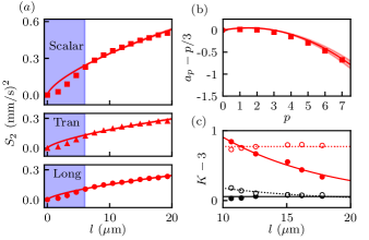
Figure 4: Numerical results. In all panels, the colors, markers, fitting and uncertainty notations follow those in Fig.3. (a) Numerical $S_{2}(l)$ obtained from the average of 40 numerical simulations. In each run, $S_{2}(l)$ was calculated using a $6\ \mathrm{\mu m}$ region of interest for $\bar{v}$ and a $3.5\ \mathrm{\mu m}$ sampling distance for collecting velocity increments. The blue region marks distances below the $\approx 6\ \mathrm{\mu m}$ resolvable distance between tracers. (b) Intermittency correction. (c) Excess Kurtosis.

Each numerical experiment began with a steady state system evolving according to Eq. (2) with an added stochastic noise term selected to give the observed $98\ \%$ condensate fraction. The simulation then followed the experimental stirring / evolution protocol, and recorded the density weighted velocity averaged over the extent of the $\approx 6\ \mu{\rm m}$ resolvable distance between tracers.

The numerical results in the remainder of Fig. 4 parallels the experimental data in Fig. 3. Panel (a) plots the second order VSFs where the blue shaded region deliniates the minimum resolvable distance between tracers. The solid curves are fits to the $2/3$ scaling law outside of this regime with amplitudes shown in Table 1. While the simulation parameter $\kappa_{0}$ was selected to match the nominal scale of these amplitudes with experiment, the close correspondence of their ratios—e.g. $s^{T}/s^{L}=1.22(1)$—as well as the overall scaling behavior are intrinsic outcomes of the simulation. Figure 4b continues by showing the intermittency corrections $\varepsilon_{p}$ from scalar VSFs (red squares) are consistent with the KO62 theory (solid curve) with an intermittency exponent $\chi$ about half that of experiment (Table 1). Panel (c) shows that, as with experiment, $K-3$ increases from zero in the turbulent case, although with a significant reduction in overall magnitude. As observed experimentally, the transverse excess kurtosis falls with increasing $l$, and the longitudinal $K-3$ remains independent of $l$.

Taken together these numerical results confirm the presence of Kolmogorov-type turbulence in this system, and provide near quantitative agreement with our experiment [this is quite surprising given the ad-hoc introduction of dissipation in to Eq. (2)].

Discussion and outlook—Here we developed and validated PIV for quantum gas experiments; although not universally applicable—as it requires access to an internal state with scattering properties similar to that of the main system—this technique has broad utility: from BEC in inhomogeneous traps to spinor scenarios, including Rayleigh-Taylor and Kelvin-Helmholtz instabilities Sasaki et al. (2009); Takeuchi et al. (2010); Kobyakov et al. (2014). In a more broad context this method is applicable to fluid dynamics in “acoustic cosmological” contexts with analog singularities Fischer and Datta (2023) and Kerr black holes Takeuchi et al. (2008) predicted.

Although PIV enabled us to demonstrate key aspects of Kolmogorov turbulence in an atomic BEC, many questions are unanswered. For example, why—both in experiment and numerics—does ${\rm PDF}(\Delta v^{L})$ have an excess kurtosis that is independent of separation? What is the relation between scaling observed from VSFs and that obtained from TOF momentum distributions Thompson et al. (2013); Navon et al. (2016)? Additionally, our studies focused on decaying turbulence in which a turbulent state is in the process of relaxing; this is in contrast with fully-developed (i.e., steady state) turbulence in which the system is continuously excited at long length scales and energy is removed at short scales. The recent development of BECs undergoing continuous replenishment and evaporation Chen et al. (2022) may enable access to this regime.

On the numerical side, the dGPE introduced dissipation in an experimentally motivated, but ultimately heuristic manner. Full 3D simulations including realistic modeling of the evaporation processes would eliminate the need for heuristics, and also inform more realistic approximate 2D descriptions. Such simulations would help connect our results to those inferring turbulence from momentum distributions Thompson et al. (2013), that found agreement with wave- rather than Kolmogorov turbulence.