DyGMamba: Efficiently Modeling Long-Term Temporal Dependency on Continuous-Time Dynamic Graphs with State Space Models

Abstract

Learning useful representations for continuous-time dynamic graphs (CTDGs) is challenging, due to the concurrent need to span long node interaction histories and grasp nuanced temporal details. In particular, two problems emerge: (1) Encoding longer histories requires more computational resources, making it crucial for CTDG models to maintain low computational complexity to ensure efficiency; (2) Meanwhile, more powerful models are needed to identify and select the most critical temporal information within the extended context provided by longer histories. To address these problems, we propose a CTDG representation learning model named DyGMamba, originating from the popular Mamba state space model (SSM). DyGMamba first leverages a node-level SSM to encode the sequence of historical node interactions. Another time-level SSM is then employed to exploit the temporal patterns hidden in the historical graph, where its output is used to dynamically select the critical information from the interaction history. We validate DyGMamba experimentally on the dynamic link prediction task. The results show that our model achieves state-of-the-art in most cases. DyGMamba also maintains high efficiency in terms of computational resources, making it possible to capture long temporal dependencies with a limited computation budget.

1 Introduction

Dynamic graphs store node interactions in the form of links labeled with timestamps (Kazemi et al., 2020). In recent years, learning dynamic graphs has gained increasing interest since it can be used to facilitate various real-world applications, e.g., social network analysis (Huo et al., 2018) and recommender system development (Wang et al., 2023). Dynamic graphs can be classified into two types, i.e., discrete-time dynamic graph (DTDG) and continuous-time dynamic graph (CTDG). A DTDG is represented as a sequence of graph snapshots that are observed at regular time intervals, where all the edges in a snapshot are taken as existing simultaneously, while a CTDG consists of a stream of events where each of them is observed individually with its own timestamp. Previous work (Kazemi et al., 2020) has indicated that CTDGs have an advantage over DTDGs in preserving temporal details, and therefore, more attention is paid to developing novel CTDG modeling approaches for dynamic graph representation learning.

Recent effort in CTDG modeling has resulted in a wide range of models (Trivedi et al., 2019; Xu et al., 2020; Rossi et al., 2020; Cong et al., 2023). However, most of these methods are unable to model long-term temporal dependencies of nodes. To solve this problem, (Yu et al., 2023) proposes a CTDG model DyGFormer that can handle long-term node interaction histories based on Transformer (Vaswani et al., 2017). Despite its ability in modeling longer histories, employing a Transformer naturally introduces excessive usage of computational resources due to its quadratic complexity. Another recent work CTAN (Gravina et al., 2024) tries to capture long-term temporal dependencies by propagating graph information in a non-dissipative way over time with a graph convolution-based model. Despite the model’s high efficiency, (Gravina et al., 2024) shows that it cannot capture very long histories and is surpassed by (Yu et al., 2023) on the CTDGs where learning from very far away temporal information is critical. Based on these observations, we summarize the first challenge in CTDG modeling: How to develop a model that is scalable in modeling very long-term historical interactions? Another point worth noting is that as longer histories introduce more temporal information, more powerful models are needed to identify and select the most critical parts. This reveals another challenge: How to effectively select critical temporal information with long node interaction histories?

To address the first challenge, we propose to leverage a currently popular state space model (SSM), i.e., Mamba SSM (Gu & Dao, 2023) to encode the long sequence of historical node interactions. Since Mamba is proven effective and efficient in long sequence modeling (Gu & Dao, 2023), it maintains low computational complexity and is scalable in modeling long-term temporal dependencies. For the second challenge, we address it by learning temporal patterns of node interactions and dynamically select the critical temporal information based on them. The motivation can be explained by the following example. Consider a CTDG with nodes as people or songs and edges representing a person playing a song at a specific time. If a person $u$ frequently plays a hit song $v$ initially but decreases the frequency as $v$’s popularity declines, the time intervals between plays increase. This increasing interval forms a temporal pattern for the edge $(u,v,t)$ between $u$ and $v$ at a future timestamp $t$. Ignoring this pattern can lead models to incorrectly predict that $u$ will still play $v$ at future timestamps due to their high appearances in each other’s historical interactions, resulting in poor performance. However, if a CTDG model is aware of this pattern, it can be a hint for the model to pay less attention to the interactions between $u$ and $v$, and select other part of temporal information which are more contributive in making correct predictions (e.g., $u$ starts to listen to another song $v^{\prime}$ a lot before $t$). Since each of such pattern corresponds to a specific edge, e.g., $(u,v,t)$, we name these patterns as edge-specific temporal patterns.

To this end, we propose a new CTDG model named DyGMamba. DyGMamba first leverages a node-level Mamba SSM to encode historical node interactions. Another time-level Mamba SSM is then employed to exploit the edge-specific temporal patterns, where its output is used to dynamically select the critical information from the interaction history. To summarize: (1) We present DyGMamba, the first model using SSMs for CTDG representation learning; (2) DyGMamba demonstrates high efficiency in modeling long-term temporal dependencies in CTDGs; (3) Experimental results show that DyGMamba achieves new state-of-the-art on dynamic link prediction over most commonly-used CTDG datasets. It shows even stronger superiority as the dataset requires longer temporal dependency.

2 Related Work and Preliminaries

2.1 Related Work

Dynamic Graph Representation Learning.

Dynamic graph representation learning methods can be categorized into two groups, i.e., DTDG and CTDG methods. DTDG methods (Pareja et al., 2020; Goyal et al., 2020; Sankar et al., 2020; You et al., 2022; Li et al., 2024) can only model DTDGs where each of them is represented as a sequence of graph snapshots. Modeling a dynamic graph as graph snapshots require time discretization and will inevitably cause information loss (Kazemi et al., 2020). To overcome this problem, recent works focus more on developing CTDG methods that treat a dynamic graph as a stream of events, where each event has its own unique timestamp. Some works (Trivedi et al., 2019; Chang et al., 2020) model CTDGs by using temporal point process. Another line of works (Xu et al., 2020; Ma et al., 2020; Wang et al., 2021b; Gravina et al., 2024; Petrović et al., 2024) designs advanced temporal graph neural networks for CTDGs. Besides, some other methods are developed based on memory networks (Kumar et al., 2019; Rossi et al., 2020; Liu et al., 2022), temporal random walk (Wang et al., 2021c; Jin et al., 2022) and temporal sequence modeling (Wang et al., 2021a; Cong et al., 2023; Yu et al., 2023; Besta et al., 2023; Tian et al., 2024). Since some real-world CTDGs heavily rely on long-term temporal information for effective learning, a number of works start to study how to build CTDG models that can do long range propagation of information over time (Yu et al., 2023; Gravina et al., 2024). We compare them later in experiments with DyGMamba to show our model outperforms them in capturing long-term temporal information.

State Space Models.

Transformer (Vaswani et al., 2017) is a de facto backbone architecture in modern deep learning. However, its self-attention mechanism results in large space and time complexity, making it unsuitable for long sequence modeling (Duman Keles et al., 2023). To address this, many works focus on building structured state space models that scale linearly or near-linearly with input sequence length (Gu et al., 2021; 2022b; 2022a; Smith et al., 2023; Peng et al., 2023; Ma et al., 2023; Gu & Dao, 2023). Most structured SSMs exhibit linear time invariance (LTI), meaning their parameters are not input-dependent and fixed for all time-steps. (Gu & Dao, 2023) demonstrates that LTI prevents SSMs from effectively selecting relevant information from the input context, which is problematic for tasks requiring context-aware reasoning. To solve this issue, (Gu & Dao, 2023) proposes S6, also known as Mamba, which uses a selection mechanism to dynamically choose important information from input sequence elements. Selection mechanism involves learning functions that map input data to the SSM’s parameters, making Mamba both efficient and effective in modeling language, DNA sequences, and audio. Recently, there have been several works employing Mamba SSM for representation learning on static graphs (Wang et al., 2024; Behrouz & Hashemi, 2024), however, they are not designed for dynamic graphs. Another work (Li et al., 2024) conducts a preliminary study on DTDG modeling with SSMs but it cannot be generalized to CTDGs.

2.2 Preliminaries

CTDG and Task Formulation.

We define CTDG and dynamic link prediction as follows.

Definition 1 (Continuous-Time Dynamic Graph).

Let $\mathcal{N}$ and $\mathcal{T}$ denote a set of nodes and timestamps, respectively. A CTDG is a sequence of $|\mathcal{G}|$ chronological interactions $\mathcal{G}=\{(u_{i},v_{i},t_{i})\}_{i=1}^{|\mathcal{G}|}$ with $0\leq t_{1}\leq t_{2}\leq...\leq t_{|\mathcal{G}|}$, where $u_{i},v_{i}\in\mathcal{N}$ are the source and destination node of the $i$-th interaction happening at $t_{i}\in\mathcal{T}$, respectively. Each node $u\in\mathcal{N}$ can be equipped with a node feature $\mathbf{x}_{u}\in\mathbb{R}^{d_{N}}$, and each interaction $(u,v,t)$ can be associated with a link (edge) feature $\mathbf{e}_{u,v}^{t}\in\mathbb{R}^{d_{E}}$. If $\mathcal{G}$ is not attributed, we set node and link features to zero vectors.

Definition 2 (Dynamic Link Prediction).

Given a CTDG $\mathcal{G}$, a source node $u\in\mathcal{N}$, a destination node $v\in\mathcal{N}$, a timestamp $t\in\mathcal{T}$, and all the interactions before $t$, i.e., $\{(u_{i},v_{i},t_{i})|t_{i}<t,(u_{i},v_{i},t_{i})\in\mathcal{G}\}$, dynamic link prediction aims to predict whether the interaction $(u,v,t)$ exists.

S4 and Mamba SSM.

A structured SSM (Gu et al., 2022b) is inspired by a continuous system described below:

$$\mathbf{z}(\tau)^{\prime}=\mathbf{A}\mathbf{z}(\tau)+\mathbf{B}q(\tau),\ \ r(\tau)=\mathbf{C}\mathbf{z}(\tau).$$ (1a)

$q(\tau)\in\mathbb{R}$ and $r(\tau)\in\mathbb{R}$ are the 1-dimensional input and output over time $\tau$, respectively. $\mathbf{A}\in\mathbb{R}^{d_{1}\times d_{1}},\mathbf{B}\in\mathbb{R}^{1\times d_{1}},\mathbf{C}\in\mathbb{R}^{d_{1}\times 1}$ are three parameters deciding the system. Based on it, a structured SSM, i.e., S4 (Gu et al., 2022b), includes a time-scale parameter $\Delta\in\mathbb{R}$ and discretizes all the parameters to adapt the model to processing sequences recurrently.

$$\mathbf{z}_{\tau}=\bar{\mathbf{A}}\mathbf{z}_{\tau-1}+\bar{\mathbf{B}}p_{\tau},\ \ q_{\tau}=\mathbf{C}\mathbf{z}_{\tau},$$ (2)

where $$\bar{\mathbf{A}}=\text{exp}(\Delta\mathbf{A}),\ \ \bar{\mathbf{B}}=(\Delta\mathbf{A})^{-1}\text{exp}((\Delta\mathbf{A})-\mathbf{I})\Delta\mathbf{B}.$$

Here, $\tau$ is also discretized to denote the position of an element in a sequence. When the dimension size of an input $d_{2}$ becomes higher (i.e., $d_{2}>1$), S4 is in a Single-Input Single-Output (SISO) fashion, processing each input dimension in parallel with the same set of parameters. Based on S4, Mamba SSM follows the SISO mode but changes its parameters into input-dependent by employing several trainable linear layers to map input into $\bar{\mathbf{A}}$, $\bar{\mathbf{B}}$ and $\Delta$. The system is evolving as it processes input data sequentially, making Mamba time-variant and suitable for modeling temporal sequences.

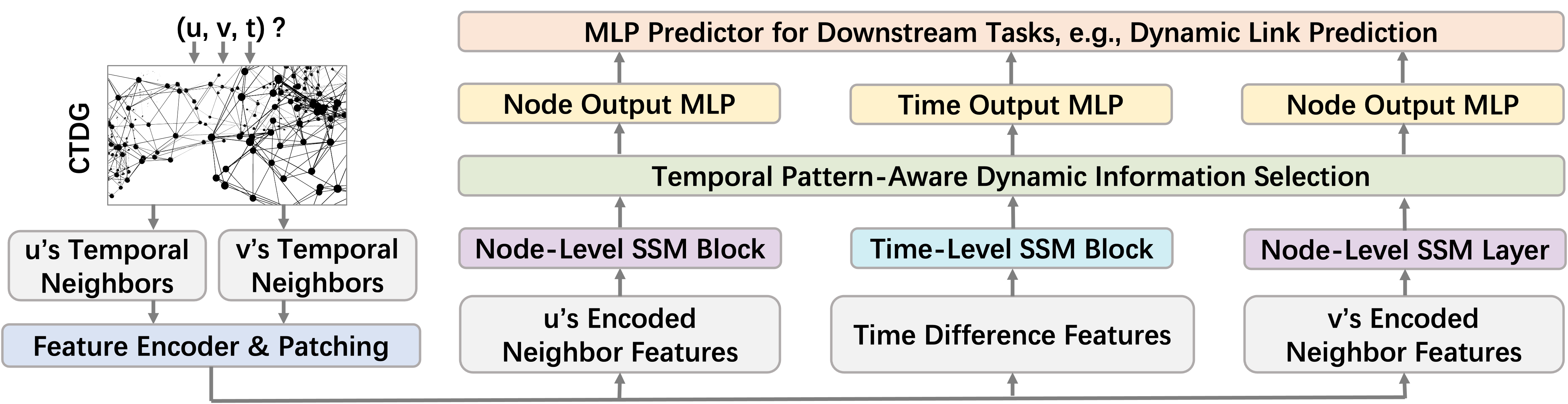
Figure 1: Model overview of DyGMamba.

3 DyGMamba

Figure 1 illustrates the overview of DyGMamba. Given a potential interaction $(u,v,t)$, CTDG models are asked to predict whether it exists or not. DyGMamba extracts the historical one-hop interactions of node $u$ and $v$ before timestamp $t$ from the CTDG $\mathcal{G}$ and gets two interaction sequences $\mathcal{S}_{u}^{t}=\{(u,u^{\prime},t^{\prime})|t^{\prime}<t,(u,u^{\prime},t^{\prime})\in\mathcal{G}\}\cup\{(u^{\prime},u,t^{\prime})|t^{\prime}<t,(u^{\prime},u,t^{\prime})\in\mathcal{G}\}$ and $\mathcal{S}_{v}^{t}=\{(v,v^{\prime},t^{\prime})|t^{\prime}<t,(v,v^{\prime},t^{\prime})\in\mathcal{G}\}\cup\{(v^{\prime},v,t^{\prime})|t^{\prime}<t,(v^{\prime},v,t^{\prime})\in\mathcal{G}\}$ containing $u$’s and $v$’s one-hop temporal neighbors $\textit{Nei}_{u}^{t}=\{(u^{\prime},t^{\prime})|(u,u^{\prime},t^{\prime})\text{ or }(u^{\prime},u,t^{\prime})\in\mathcal{G},t^{\prime}<t\}$ and $\textit{Nei}_{v}^{t}=\{(v^{\prime},t^{\prime})|(v,v^{\prime},t^{\prime})\text{ or }(v^{\prime},v,t^{\prime})\in\mathcal{G}\}$ (link features are omitted for clarity). Then it encodes the neighbors in $\textit{Nei}_{u}^{t}$ and $\textit{Nei}_{v}^{t}$ to get two sequences of encoded neighbor representations for $u$ and $v$. To learn the edge-specific temporal pattern of $(u,v,t)$, we find the interactions between $u$ and $v$ before $t$, compute the time difference between each pair of neighboring interactions, and build a sequence of time differences $\mathcal{S}_{u,v}^{t}$. Finally, DyGMamba dynamically selects critical information from the encoded neighbors and incorporates the learned temporal pattern to achieve link prediction.

3.1 Learning One-Hop Temporal Neighbors

Encode Neighbor Features.

Given one-hop temporal neighbors $\textit{Nei}_{u}^{t}$ of the source node $u$, we sort them in the chronological order and append $(u,t)$ at the end to form a sequence of $\textit{Nei}_{u}^{t}+1$ temporal nodes. We take their node features from the dataset and stack them into a feature matrix $\tilde{\mathbf{X}}_{u}^{t}\in\mathbb{R}^{(|\textit{Nei}_{u}^{t}|+1)\times d_{N}}$. Similarly, we build a link feature matrix $\tilde{\mathbf{E}}_{u}^{t}\in\mathbb{R}^{(|\textit{Nei}_{u}^{t}|+1)\times d_{E}}$. To incorporate temporal information, we encode the time difference between $u$ and each one-hop temporal neighbor $(u^{\prime},t^{\prime})$ using the time encoding function introduced in TGAT (Xu et al., 2020): $\sqrt{1/d_{T}}[cos(\omega_{1}(t-t^{\prime})+\phi_{1}),\dots,cos(\omega_{d}(t-t^{\prime})+\phi_{d_{T}})]$, where $d_{T}$ is the dimension of time representation, $\omega_{1}\dots\omega_{d_{T}}$ and $\phi_{1}\dots\phi_{d_{T}}$ are trainable parameters. The time feature of $u$’s temporal neighbors are denoted as $\tilde{\mathbf{T}}_{u}^{t}\in\mathbb{R}^{(|\textit{Nei}_{u}^{t}|+1)\times d_{T}}$. We follow the same way to get $\tilde{\mathbf{X}}_{v}^{t}\in\mathbb{R}^{(|\textit{Nei}_{v}^{t}|+1)\times d_{N}}$, $\tilde{\mathbf{E}}_{v}^{t}\in\mathbb{R}^{(|\textit{Nei}_{v}^{t}|+1)\times d_{E}}$ and $\mathbf{T}_{v}^{t}\in\mathbb{R}^{(|\textit{Nei}_{v}^{t}|+1)\times d_{T}}$ for $v$’s temporal neighbors. Following (Tian et al., 2024), we also consider the historical node interaction frequencies in the interaction sequences $\mathcal{S}_{u}^{t}$ and $\mathcal{S}_{v}^{t}$ of source $u$ and destination $v$. For example, assume the interacted nodes of $u$ and $v$ (arranged in chronological order) are $\{a,v,a\}$ and $\{b,b,u,a\}$, the appearing frequencies of $a$, $b$ in $u$/$v$’s historical interactions are 2/1, 0/2, respectively. And the frequency of the interaction involving $u$ and $v$ is 1. Thus, the node interaction frequency features of $u$ and $v$ are written as $\tilde{F}_{u}^{t}=[[2,1],[1,1],[2,1],[0,1]]^{\top}$ and $\tilde{F}_{v}^{t}=[[0,2],[0,2],[1,1],[2,1],[0,1]]^{\top}$, respectively. Note that the last elements ($[0,1]$ and $[0,1]$) in $\tilde{F}_{u}^{t}$ and $\tilde{F}_{v}^{t}$ correspond to the appended $(u,t)$ and $(v,t)$ not existing in the observed histories. We initialize them with $[0,\textit{number of historical interactions between}\ u,v]$. An encoding multilayer perceptron (MLP) $f(\cdot):\mathbb{R}\to\mathbb{R}^{d_{F}}$ is employed to encode these features into representations: $\tilde{\mathbf{F}}_{u}^{t}=f(\tilde{F}_{u}^{t}[:,0])+f(\tilde{F}_{u}^{t}[:,1])\in\mathbb{R}^{(|\textit{Nei}_{u}^{t}|+1)\times d_{F}}$, $\tilde{\mathbf{F}}_{v}^{t}=f(\tilde{F}_{v}^{t}[:,0])+f(\tilde{F}_{v}^{t}[:,1])\in\mathbb{R}^{(|\textit{Nei}_{v}^{t}|+1)\times d_{F}}$.

Patching Neighbors.

We employ the patching technique proposed by (Yu et al., 2023) to save computational resources when dealing with a large number of temporal neighbors. We treat $p$ temporally adjacent neighbors as a patch and flatten their features. For example, with patching, $\tilde{\mathbf{X}}_{u}^{t}\in\mathbb{R}^{(|\textit{Nei}_{u}^{t}|+1)\times d_{N}}$ results in a new patched feature matrix $\mathbf{X}_{u}^{t}\in\mathbb{R}^{\lceil(|\textit{Nei}_{u}^{t}|+1)/p\rceil\times(p\cdot d_{N})}$ (we pad $\tilde{\mathbf{X}}_{u}^{t}$ with zero-valued features when $|\textit{Nei}_{u}^{t}|+1$ cannot be divided by $p$). Similarly, we get $\mathbf{X}_{\theta}^{t}\in\mathbb{R}^{\lceil(|\textit{Nei}_{\theta}^{t}|+1)/p\rceil\times(p\cdot d_{N})}$, $\mathbf{E}_{\theta}^{t}\in\mathbb{R}^{\lceil(|\textit{Nei}_{\theta}^{t}|+1)/p\rceil\times(p\cdot d_{E})}$, $\mathbf{T}_{\theta}^{t}\in\mathbb{R}^{\lceil(|\textit{Nei}_{\theta}^{t}|+1)/p\rceil\times(p\cdot d_{T})}$ and $\mathbf{F}_{\theta}^{t}\in\mathbb{R}^{\lceil(|\textit{Nei}_{\theta}^{t}|+1)/p\rceil\times(p\cdot d_{F})}$ ($\theta$ is either $u$ or $v$). Each row of a feature matrix (whether before or after patching) corresponds to an element of the input sequence sent into an SSM later. Recall that SSMs process sequences in a recurrent way. Patching decreases the length of the sequence by roughly $p$ times, making great contribution in saving computational resources.

Node-Level SSM Block.

We first map the padded features of $u$’s and $v$’s one-hop temporal neighbors to the same dimension $d$:

$$\mathbf{X}_{\theta}^{t}:=f_{N}(\mathbf{X}_{\theta}^{t}),\ \ \mathbf{E}_{\theta}^{t}:=f_{E}(\mathbf{E}_{\theta}^{t}),\ \ \mathbf{T}_{\theta}^{t}:=f_{T}(\mathbf{T}_{\theta}^{t}),\ \ \mathbf{F}_{\theta}^{t}:=f_{F}(\mathbf{F}_{\theta}^{t}).$$ (3)

$f_{N}(\cdot):\mathbb{R}^{p\cdot d_{N}}\to\mathbb{R}^{d}$, $f_{E}(\cdot):\mathbb{R}^{p\cdot d_{E}}\to\mathbb{R}^{d}$, $f_{T}(\cdot):\mathbb{R}^{p\cdot d_{T}}\to\mathbb{R}^{d}$, $f_{F}(\cdot):\mathbb{R}^{p\cdot d_{F}}\to\mathbb{R}^{d}$ are four MLPs for different types of neighbor features. We take the concatenation of them as the encoded representations of the temporal neighbors, i.e., $\mathbf{H}_{\theta}^{t}=\mathbf{X}_{\theta}^{t}\|\mathbf{E}_{\theta}^{t}\|\mathbf{T}_{\theta}^{t}\|\mathbf{F}_{\theta}^{t}\in\mathbb{R}^{\lceil(|\textit{Nei}_{\theta}^{t}|+1)/p\rceil\times 4d}$. We input $\mathbf{H}_{u}^{t}$ and $\mathbf{H}_{v}^{t}$ separately into a node-level SSM block to learn the temporal dependencies of temporal neighbors. The node-level SSM block consists of $l_{N}$ layers, where each layer is defined as follows (Eq. 4-5). First, we input $\mathbf{H}_{\theta}^{t}$ into a Mamba SSM

$$\mathbf{B}_{1}=\mathbf{H}_{\theta}^{t}\mathbf{W}_{\mathbf{B}_{1}}\in\mathbb{R}^{\lceil(|\textit{Nei}_{\theta}^{t}|+1)/p\rceil\times d_{\text{SSM}}},\ \ \mathbf{C}_{1}=\mathbf{H}_{\theta}^{t}\mathbf{W}_{\mathbf{C}_{1}}\in\mathbb{R}^{\lceil(|\textit{Nei}_{\theta}^{t}|+1)/p\rceil\times d_{\text{SSM}}};$$ (4a)

$$\Delta_{1}=\text{Softplus}(\text{Broadcast}_{4d}(\mathbf{H}_{\theta}^{t}\mathbf{W}_{\Delta_{1}})+\text{Param}_{\Delta_{1}})\in\mathbb{R}^{\lceil(|\textit{Nei}_{\theta}^{t}|+1)/p\rceil\times 4d};$$ (4b)

$$\bar{\mathbf{A}}_{1}=\text{exp}(\Delta_{1}\mathbf{A}_{1}),\ \ \bar{\mathbf{B}}_{1}=(\Delta_{1}\mathbf{A}_{1})^{-1}\text{exp}((\Delta_{1}\mathbf{A}_{1})-\mathbf{I})\Delta_{1}\mathbf{B}_{1};$$ (4c)

$$\mathbf{H}_{\theta}^{t}:=\mathbf{H}_{\theta}^{t}+\text{SSM}_{\bar{\mathbf{A}}_{1},\bar{\mathbf{B}}_{1},\mathbf{C}_{1}}(\mathbf{H}_{\theta}^{t}).$$ (4d)

$\mathbf{W}_{\mathbf{B}_{1}},\mathbf{W}_{\mathbf{C}_{1}}\in\mathbb{R}^{4d\times d_{\text{SSM}}}$ and $\mathbf{W}_{\Delta_{1}}\in\mathbb{R}^{4d\times 1}$. $\bar{\mathbf{A}}_{1},\bar{\mathbf{B}}_{1}\in\mathbb{R}^{\lceil(|\textit{Nei}_{\theta}^{t}|+1)/p\rceil\times 4d\times d_{\text{SSM}}}$ are discretized parameters. $\text{Param}_{\Delta_{1}}\in\mathbb{R}^{\lceil(|\textit{Nei}_{\theta}^{t}|+1)/p\rceil\times 4d}$ is a parameter defined in (Gu & Dao, 2023). $\mathbf{I}$ is an identity matrix, and Eq. 4d denotes the SSM forward process similar to Eq. 2. Then we use an MLP $f_{\text{node}}(\cdot):\mathbb{R}^{4d}\to\mathbb{R}^{4d}$ on SSM’s output

$$\mathbf{H}_{\theta}^{t}:=\mathbf{H}_{\theta}^{t}+f_{\text{node}}\left(\text{LayerNorm}({\mathbf{H}_{\theta}^{t})}\right).$$ (5)

After $l_{N}$ layers, we have $\mathbf{H}_{u}^{t}$ and $\mathbf{H}_{v}^{t}$ that contain the encoded information of all one-hop temporal neighbors for the entities $u$ and $v$ as well as the information of themselves. Since we sort temporal neighbors chronologically, our node-level SSM block can directly learn the temporal dynamics for graph forecasting. Another point worth noting is that Mamba SSM is originally good at capturing long-term dependencies. Our model can benefit from this when temporally faraway neigbors are critical for decision making.

3.2 Learning from Edge-Specific Temporal Patterns

Time-Level SSM Block.

To capture edge-specific temporal patterns, we use another time-level SSM block consisting of $l_{T}$ layers. We first find out $k$ temporally nearest historical interactions between $u$ and $v$ before $t$ and sort them in the chronological order, i.e., $\{(u,v,t_{0}),...,(u,v,t_{k-1})|t_{0}<...<t_{k-1},t_{k-1}<t\}$. Then we construct a timestamp sequence $\{t_{0},t_{1},...,t_{k-1},t\}$ based on these interactions and the prediction timestamp $t$. We compute the time difference between each neighboring pair of them and further get a time difference sequence $\{t_{1}-t_{0},t_{2}-t_{1},...,t-t_{k-1}\}$, representing the change of time interval between two identical interactions. Each element in this sequence is input into the time encoding function stated above to get a edge-specific (specific to the edge $(u,v,t)$) time feature. The features are stacked into a feature matrix $\mathbf{H}_{u,v}^{t}\in\mathbb{R}^{k\times d_{T}}$ and mapped by an MLP $f_{\text{map}1}(\cdot):\mathbb{R}^{d_{T}}\to\mathbb{R}^{\gamma d}$ ($\gamma\in[0,1]$ is a hyperparameter), i.e., $\mathbf{H}_{u,v}^{t}:=f_{\text{map}1}(\mathbf{H}_{u,v}^{t})$. A time-level SSM layer takes $\mathbf{H}_{u,v}^{t}$ as input and computes

$$\mathbf{B}_{2}=\mathbf{H}_{u,v}^{t}\mathbf{W}_{\mathbf{B}_{2}}\in\mathbb{R}^{k\times d_{\text{SSM}}},\ \ \mathbf{C}_{2}=\mathbf{H}_{u,v}^{t}\mathbf{W}_{\mathbf{C}_{2}}\in\mathbb{R}^{k\times d_{\text{SSM}}};$$ (6a)

$$\Delta_{2}=\text{Softplus}(\text{Broadcast}_{\gamma d}(\mathbf{H}_{u,v}^{t}\mathbf{W}_{\Delta_{2}})+\text{Param}_{\Delta_{2}})\in\mathbb{R}^{k\times\gamma d};$$ (6b)

$$\bar{\mathbf{A}}_{2}=\text{exp}(\Delta_{2}\mathbf{A}_{2}),\ \ \bar{\mathbf{B}}_{2}=(\Delta_{2}\mathbf{A}_{2})^{-1}\text{exp}((\Delta_{2}\mathbf{A}_{2})-\mathbf{I})\Delta_{2}\mathbf{B}_{2};$$ (6c)

$$\mathbf{H}_{u,v}^{t}:=\mathbf{H}_{u,v}^{t}+\text{SSM}_{\bar{\mathbf{A}}_{2},\bar{\mathbf{B}}_{2},\mathbf{C}_{2}}(\mathbf{H}_{u,v}^{t}).$$ (6d)

$\mathbf{W}_{\mathbf{B}_{2}},\mathbf{W}_{\mathbf{C}_{2}}\in\mathbb{R}^{\gamma d\times d_{\text{SSM}}}$ and $\mathbf{W}_{\Delta_{2}}\in\mathbb{R}^{\gamma d\times 1}$. $\bar{\mathbf{A}}_{2},\bar{\mathbf{B}}_{2}\in\mathbb{R}^{k\times\gamma d\times d_{\text{SSM}}}$ are discretized parameters. $\text{Param}_{\Delta_{2}}\in\mathbb{R}^{k\times\gamma d}$ is a parameter defined as same as $\text{Param}_{\Delta_{1}}$. In practice, we set $k$ to a number much smaller than $|\textit{Nei}_{\theta}^{t}|$, e.g., $10$. This ensures that time-level SSM will not incur huge computational burden and the model focuses more on the recent histories. Note that we cannot always find $k$ recent interactions between $u$ and $v$. To enable batch processing, we set the time difference without a found historical interaction to a very large number $10^{10}$. For example, if $k=2$, and for $(u,v,t)$ we can only find $(u,v,t_{0})$. The time difference sequence will be $\{10^{10},t-t_{0}\}$. $10^{10}$ is much larger than $t-t_{0}$, indicating that $u$ and $v$ have not had an interaction for an extremely long time, same as existing no historical interaction.

Dynamic Information Selection with Temporal Patterns.

After the time-level SSM block, we compute a compressed representation to represent the edge-specific temporal pattern

$$\mathbf{h}_{u,v}^{t}=\text{MeanPooling}(\mathbf{H}_{u,v}^{t}),$$ (7)

where $\text{MeanPooling}(\cdot)$ averages over $k$ interactions. As a result, we have $\mathbf{h}_{u,v}^{t}\in\mathbb{R}^{\gamma d}$ to represent the temporal pattern specific to the edge $(u,v,t)$. To leverage learned temporal pattern, we use it to dynamically select the information from node representations $\mathbf{h}_{u}^{t}$ and $\mathbf{h}_{v}^{t}$

$$\tilde{\mathbf{h}}_{u,v}^{t}=f_{\text{map}2}(\mathbf{h}_{u,v}^{t})\in\mathbb{R}^{4d};$$ (8a)

$$\tilde{\mathbf{h}}_{\theta}^{t}={\mathbf{w}_{\text{agg}}}^{\top}\mathbf{H}_{\theta}^{t}\in\mathbb{R}^{4d},\ \text{where}\ \mathbf{w}_{\text{agg}}=f_{\text{map}3}(\mathbf{H}_{\theta}^{t})\in\mathbb{R}^{|\textit{Nei}_{\theta}^{t}|+1};$$ (8b)

$$\alpha_{u}=f^{\prime}(\tilde{\mathbf{h}}_{v}^{t})*\tilde{\mathbf{h}}_{u,v}^{t}\in\mathbb{R}^{4d},\ \alpha_{v}=f^{\prime}(\tilde{\mathbf{h}}_{u}^{t})*\tilde{\mathbf{h}}_{u,v}^{t}\in\mathbb{R}^{4d};$$ (8c)

$$\mathbf{h}_{\theta}^{t}={\beta_{\theta}}^{\top}\mathbf{H}_{\theta}^{t},\ \text{where}\ \beta_{\theta}=\text{Softmax}(\mathbf{H}_{\theta}^{t}\alpha_{\theta})\in\mathbb{R}^{|\textit{Nei}_{\theta}^{t}|+1}.$$ (8d)

$f_{\text{map}2}(\cdot):\mathbb{R}^{\gamma d}\to\mathbb{R}^{4d}$ and $f_{\text{map}3}(\cdot):\mathbb{R}^{4d}\to\mathbb{R}^{1}$ are two mapping MLPs. $f_{\text{agg}}(\cdot):\mathbb{R}^{4d}\to\mathbb{R}^{4d}$ is another MLP introducing training parameters. $\alpha_{\theta}$ can be viewed as a key used to select important historical information from the node $\theta$ (either $u$ or $v$) at $t$. Note that $\alpha_{u}$/$\alpha_{v}$ is computed by considering both the edge-specific temporal pattern and the opposite node $v$/$u$. In the node-level SSM block, we separately model the one-hop temporal neighbors of each node $\theta$, making it hard to connect $u$ and $v$. Computing $\alpha_{\theta}$ as Eq. 8c helps to strengthen the connection between both nodes and meanwhile incorporates the learned temporal pattern. $\beta_{\theta}$ is derived by transforming the queried results based on $\alpha_{\theta}$ into weights. It is then used to compute a weighted-sum of all temporal neighbors for representing $\theta$ at $t$, i.e., $\mathbf{h}_{\theta}^{t}$. Finally, we output the representations of $u$, $v$ and the edge-specific temporal pattern by employing two output MLPs $f_{\text{out}1}(\cdot):\mathbb{R}^{4d}\to\mathbb{R}^{d_{N}}$ and $f_{\text{out}2}(\cdot):\mathbb{R}^{\gamma d}\to\mathbb{R}^{d_{N}}$

$$\mathbf{h}_{\theta}^{t}:=f_{\text{out}1}(\mathbf{h}_{\theta}^{t})\in\mathbb{R}^{d_{N}},\ \mathbf{h}_{u,v}^{t}:=f_{\text{out}2}(\mathbf{h}_{u,v}^{t})\in\mathbb{R}^{d_{N}}.$$ (9)

3.3 Leveraging Learned Representations for Link Prediction

We leverage $\mathbf{h}_{\theta}^{t}$ and $\mathbf{h}_{u,v}^{t}$ for dynamic link prediction. We employ a prediction MLP, i.e., $f_{\text{LP}}(\cdot):\mathbb{R}^{3d_{N}}\to\mathbb{R}$, as the predictor. The probability of existing a link $(u,v,t)$ is computed as $\hat{y}(u,v,t)=\text{Sigmoid}(f_{\text{LP}}(\mathbf{h}_{u}^{t}\|\mathbf{h}_{v}^{t}\|\mathbf{h}_{u,v}^{t}))$. For model parameter learning, we use the following loss function

$$\mathcal{L}=-\frac{1}{2M}\sum_{2M}\left(y(u,v,t)\log(\hat{y}(u,v,t))+(1-y(u,v,t))\log(1-\hat{y}(u,v,t))\right).$$ (10)

$y(u,v,t)$ is the ground truth label denoting the existence of $(u,v,t)$ ($1$/$0$ means existing/non-existing). $M$ is the total number of edges existing in the training data (positive edges). We follow previous work (Yu et al., 2023) and randomly sample one negative edge for each positive edge during training. Therefore, in total we have $2M$ edges considered in our loss $\mathcal{L}$.

4 Experiments

In Sec. 4.2, we validate DyGMamba’s ability in CTDG representation learning by comparing it with baseline methods on dynamic link prediction, and present ablation studies to demonstrate the effectiveness of model components. In Sec. 4.3, we further show DyGMamba’s efficiency in terms of model size, training time and GPU memory consumption. We also show that DyGMamba achieves much stronger scalability in modeling long-term temporal information compared with DyGFormer.

4.1 Experimental Setting

CTDG Datasets and Baselines.

We consider seven real-world CTDG datasets collected by (Poursafaei et al., 2022), i.e., LastFM, Enron, MOOC, Reddit, Wikipedia, UCI and Social Evo.. Dataset statistics are presented in App. B. Among them, we take LastFM, Enron and MOOC as long-range temporal dependent datasets because according to (Yu et al., 2023), much longer histories are needed for optimal representation learning on them. We compare DyGMamba with ten recent CTDG baseline models, i.e., JODIE (Kumar et al., 2019), DyRep (Trivedi et al., 2019), TGAT (Xu et al., 2020), TGN (Rossi et al., 2020), CAWN (Wang et al., 2021c), EdgeBank (Poursafaei et al., 2022), TCL (Wang et al., 2021a), GraphMixer (Cong et al., 2023), DyGFormer (Yu et al., 2023) and CTAN (Gravina et al., 2024). Among them, only DyGFormer and CTAN are designed for long-range temporal information propagation. Detailed descriptions of baseline methods are presented in App. C. We also implemented FreeDyG (Tian et al., 2024) by using its official code repository, however, on LastFM, we find that FreeDyG’s loss cannot converge and the reported results are not reproducible. So we do not report its performance in our paper.

Evaluation Settings and Metrics.

We employ two evaluation settings following previous works: the transductive and inductive settings. In the transductive setting, models are asked to predict the future links between the nodes that have been seen during training, while in the inductive setting, models should predict the links between previously unseen nodes. As suggested in (Poursafaei et al., 2022), we do link prediction evaluation using three negative sampling strategies (NSSs): random, historical and inductive. Historical NSS is only considered under the transductive setting. See App. E for detailed explanations. We employ two metrics, i.e., average precision (AP) and area under the receiver operating characteristic curve (AUC-ROC) We chronologically split each dataset with the ratio of 70%/15%/15% for training/validation/testing.

Implementation Details.

We use the implementations and the best hyperparameters provided by (Yu et al., 2023) for all baseline models except CTAN. For CTAN, we use its official implementation, fixing the number of layers to 5. All models are trained with a batch size of 200 for fair efficiency analysis. For DyGMamba, we report the number of sampled one-hop temporal neighbors $\rho$ and the patch size $p$ here. On Wikipedia, Social Evo., and UCI, $\rho\ \&\ p=32\ \&\ 1$. On Reddit, $\rho\ \&\ p=64\ \&\ 2$. On MOOC, $\rho\ \&\ p=128\ \&\ 4$. On Enron, $\rho\ \&\ p=256\ \&\ 8$. On LastFM, $\rho\ \&\ p=512\&16$. Note that to fairly compare DyGMamba’s efficiency with DyGFormer, we keep the sequence length $\rho/p$ input into the SSM as same as the length input into Transformer in (Yu et al., 2023), i.e., $\rho/p=32$. All experiments are implemented with PyTorch (Paszke et al., 2019) on a server equipped with an AMD EPYC 7513 32-Core Processor and a single NVIDIA A40 with 45GB memory. We run each experiment for five times with five random seeds and report the mean results together with error bars. We report further implementation details including complete hyperparamter configurations in App. D.

Table 1: AP of transductive dynamic link prediction. The best and the second best results are marked as bold and underlined, respectively. CTAN cannot be trained before 120 hours timeout on Social Evo. so is ranked bottom on this dataset.

NSS

Datasets

JODIE

DyRep

TGAT

TGN

CAWN

EdgeBank

TCL

GraphMixer

DyGFormer

CTAN

DyGMamba

Random

LastFM

70.95 $\pm$ 2.94

71.85 $\pm$ 2.44

73.30 $\pm$ 0.18

75.31 $\pm$ 5.62

86.60 $\pm$ 0.11

79.29 $\pm$ 0.00

76.62 $\pm$ 1.83

75.56 $\pm$ 0.19

92.95 $\pm$ 0.14

86.44 $\pm$ 0.80

93.35 $\pm$ 0.20

Enron

84.85 $\pm$ 3.13

79.80 $\pm$ 2.28

70.76 $\pm$ 1.05

86.98 $\pm$ 1.05

89.50 $\pm$ 0.10

83.53 $\pm$ 0.00

85.41 $\pm$ 0.71

82.13 $\pm$ 0.30

92.42 $\pm$ 0.11

92.52 $\pm$ 1.20

92.65 $\pm$ 0.12

MOOC

81.04 $\pm$ 0.83

81.50 $\pm$ 0.77

85.71 $\pm$ 0.20

89.15 $\pm$ 1.69

80.30 $\pm$ 0.43

57.97 $\pm$ 0.00

83.89 $\pm$ 0.86

82.80 $\pm$ 0.15

87.66 $\pm$ 0.48

84.71 $\pm$ 2.85

89.21 $\pm$ 0.08

Reddit

98.31 $\pm$ 0.06

98.18 $\pm$ 0.03

98.57 $\pm$ 0.01

98.65 $\pm$ 0.04

99.11 $\pm$ 0.01

94.86 $\pm$ 0.00

97.78 $\pm$ 0.02

97.31 $\pm$ 0.01

99.22 $\pm$ 0.01

97.21 $\pm$ 0.84

99.32 $\pm$ 0.01

Wikipedia

96.51 $\pm$ 0.22

94.88 $\pm$ 0.29

96.88 $\pm$ 0.06

98.45 $\pm$ 0.10

98.77 $\pm$ 0.01

90.37 $\pm$ 0.00

97.75 $\pm$ 0.04

97.22 $\pm$ 0.02

99.03 $\pm$ 0.03

96.61 $\pm$ 0.79

99.15 $\pm$ 0.02

UCI

89.28 $\pm$ 1.02

66.11 $\pm$ 2.75

79.40 $\pm$ 0.61

92.33 $\pm$ 0.64

95.13 $\pm$ 0.23

76.20 $\pm$ 0.00

86.63 $\pm$ 1.30

93.15 $\pm$ 0.41

95.74 $\pm$ 0.17

76.64 $\pm$ 4.11

95.91 $\pm$ 0.15

Social Evo.

89.88 $\pm$ 0.40

88.39 $\pm$ 0.69

93.33 $\pm$ 0.06

93.45 $\pm$ 0.29

84.90 $\pm$ 0.11

74.95 $\pm$ 0.00

93.82 $\pm$ 0.19

93.36 $\pm$ 0.06

94.63 $\pm$ 0.07

Timeout

94.77 $\pm$ 0.01

Avg. Rank

8.29

9.29

7.00

4.29

6.00

9.43

5.57

6.43

2.43

6.29

1.00

Historical

LastFM

74.38 $\pm$ 6.27

71.85 $\pm$ 2.91

71.60 $\pm$ 0.36

75.03 $\pm$ 6.90

69.93 $\pm$ 0.33

73.03 $\pm$ 0.00

71.02 $\pm$ 2.07

72.28 $\pm$ 0.37

81.51 $\pm$ 0.14

82.29 $\pm$ 0.94

83.02 $\pm$ 0.16

Enron

69.13 $\pm$ 1.66

72.58 $\pm$ 1.83

64.24 $\pm$ 1.24

74.31 $\pm$ 0.99

65.40 $\pm$ 0.36

76.53 $\pm$ 0.00

72.39 $\pm$ 0.61

77.35 $\pm$ 1.22

76.93 $\pm$ 0.76

77.24 $\pm$ 1.53

77.77 $\pm$ 1.32

MOOC

78.62 $\pm$ 2.43

75.14 $\pm$ 2.86

82.83 $\pm$ 0.71

85.46 $\pm$ 2.32

74.46 $\pm$ 0.53

60.71 $\pm$ 0.00

78.51 $\pm$ 1.24

77.09 $\pm$ 0.83

85.65 $\pm$ 0.89

67.73 $\pm$ 2.08

85.89 $\pm$ 0.94

Reddit

79.96 $\pm$ 0.30

79.40 $\pm$ 0.30

79.78 $\pm$ 0.25

81.05 $\pm$ 0.32

80.96 $\pm$ 0.28

73.59 $\pm$ 0.00

77.38 $\pm$ 0.20

78.39 $\pm$ 0.40

81.63 $\pm$ 1.08

89.77 $\pm$ 2.28

81.80 $\pm$ 1.52

Wikipedia

81.16 $\pm$ 0.73

79.46 $\pm$ 0.95

87.31 $\pm$ 0.36

87.31 $\pm$ 0.25

66.77 $\pm$ 6.62

73.35 $\pm$ 0.00

86.12 $\pm$ 1.69

90.74 $\pm$ 0.06

70.13 $\pm$ 11.02

95.91 $\pm$ 0.10

81.77 $\pm$ 1.20

UCI

74.77 $\pm$ 5.35

55.89 $\pm$ 2.83

66.78 $\pm$ 0.77

81.32 $\pm$ 1.26

64.69 $\pm$ 1.78

65.50 $\pm$ 0.00

74.62 $\pm$ 2.70

83.88 $\pm$ 1.06

80.44 $\pm$ 1.16

76.62 $\pm$ 0.33

81.03 $\pm$ 1.09

Social Evo.

91.26 $\pm$ 2.47

92.86 $\pm$ 0.90

95.31 $\pm$ 0.30

93.84 $\pm$ 1.68

85.65 $\pm$ 0.11

80.57 $\pm$ 0.00

95.93 $\pm$ 0.63

95.30 $\pm$ 0.34

97.05 $\pm$ 0.16

Timeout

97.35 $\pm$ 0.52

Avg. Rank

6.57

8.14

6.57

4.14

9.29

8.71

7.00

4.71

4.00

4.71

2.14

Inductive

LastFM

62.63 $\pm$ 6.89

62.49 $\pm$ 3.04

71.16 $\pm$ 0.33

65.09 $\pm$ 7.05

67.38 $\pm$ 0.57

75.49 $\pm$ 0.00

62.76 $\pm$ 0.81

67.87 $\pm$ 0.37

72.60 $\pm$ 0.06

80.06 $\pm$ 0.85

73.63 $\pm$ 0.54

Enron

69.51 $\pm$ 1.06

66.78 $\pm$ 2.21

63.16 $\pm$ 0.59

73.27 $\pm$ 0.58

75.08 $\pm$ 0.81

73.89 $\pm$ 0.00

70.98 $\pm$ 0.96

74.12 $\pm$ 0.65

78.22 $\pm$ 0.80

72.02 $\pm$ 2.64

80.86 $\pm$ 1.24

MOOC

66.56 $\pm$ 1.49

61.48 $\pm$ 0.96

76.96 $\pm$ 0.89

77.59 $\pm$ 1.83

73.55 $\pm$ 0.36

49.43 $\pm$ 0.00

76.35 $\pm$ 1.41

74.24 $\pm$ 0.75

80.99 $\pm$ 0.88

64.93 $\pm$ 3.31

81.11 $\pm$ 0.63

Reddit

86.93 $\pm$ 0.21

86.06 $\pm$ 0.36

89.93 $\pm$ 0.10

88.12 $\pm$ 0.13

91.89 $\pm$ 0.18

85.48 $\pm$ 0.00

86.97 $\pm$ 0.26

85.37 $\pm$ 0.26

91.06 $\pm$ 0.60

90.99 $\pm$ 2.19

91.15 $\pm$ 0.54

Wikipedia

74.78 $\pm$ 0.56

70.55 $\pm$ 1.22

86.77 $\pm$ 0.29

85.80 $\pm$ 0.15

69.27 $\pm$ 7.07

80.63 $\pm$ 0.00

72.54 $\pm$ 4.69

88.54 $\pm$ 0.20

62.00 $\pm$ 14.00

94.15 $\pm$ 0.08

79.86 $\pm$ 2.18

UCI

66.02 $\pm$ 1.28

54.64 $\pm$ 2.52

67.63 $\pm$ 0.51

70.34 $\pm$ 0.72

64.08 $\pm$ 1.06

57.43 $\pm$ 0.00

73.49 $\pm$ 2.21

79.57 $\pm$ 0.61

70.51 $\pm$ 1.83

66.25 $\pm$ 0.51

71.95 $\pm$ 2.51

Social Evo.

91.08 $\pm$ 3.29

92.84 $\pm$ 0.98

95.20 $\pm$ 0.30

94.58 $\pm$ 1.52

88.50 $\pm$ 0.13

83.69 $\pm$ 0.00

96.14 $\pm$ 0.63

95.11 $\pm$ 0.32

97.62 $\pm$ 0.12

Timeout

97.68 $\pm$ 0.42

Avg. Rank

8.29

9.57

5.43

5.43

6.57

7.57

6.00

5.00

4.00

5.71

2.43

4.2 Performance Analysis

Comparative Study on Benchmark Datasets.

We report the AP of transductive and inductive link prediction in Table 1 and 2 (AUC-ROC reported in Table 8 and 9 in App. F). We find that: (1) DyGMamba constantly ranks top $1$ under the random NSS, showing a superior performance; (2) Under the historical and inductive NSS, DyGMamba can achieve the best average rank compared with all baselines. More importantly, it performs much better on the datasets where encoding longer-term temporal dependencies is necessary, e.g., on LastFM, Enron and MOOC which requires larger $\rho$. This shows DyGMamba’s ability in modeling long-term temporal dependent CTDGs; (3) Among the models that can do long range propagation of information over time (i.e., DyGFormer, CTAN and DyGMamba), DyGMamba achieves the best average rank under any NSS setting in both transductive and inductive link prediction. On the long-range temporal datasets LastFM, Enron and MOOC, DyGMamba outperforms DyGFormer and CTAN in most cases; (4) CTAN achieves much better results in transductive than in inductive link prediction. This is because CTAN requires multi-hop temporal neighbors to learn node representations, which is difficult for unseen nodes. By contrast, DyGMamba and DyGFormer requires only one-hop temporal neighbors, thus performing much better in inductive link prediction.

Table 2: AP of inductive dynamic link prediction. EdgeBank cannot do inductive link prediction so is not reported.

NSS	Datasets	JODIE	DyRep	TGAT	TGN	CAWN	TCL	GraphMixer	DyGFormer	CTAN	DyGMamba
Random	LastFM	83.13 $\pm$ 1.19	83.47 $\pm$ 1.06	78.40 $\pm$ 0.30	81.18 $\pm$ 3.27	89.33 $\pm$ 0.06	81.38 $\pm$ 1.53	82.07 $\pm$ 0.31	94.17 $\pm$ 0.10	60.40 $\pm$ 3.01	94.42 $\pm$ 0.21
	Enron	78.97 $\pm$ 1.59	73.97 $\pm$ 3.00	66.67 $\pm$ 1.07	78.76 $\pm$ 1.69	86.30 $\pm$ 0.56	82.61 $\pm$ 0.61	75.55 $\pm$ 0.81	89.62 $\pm$ 0.27	74.61 $\pm$ 1.64	89.67 $\pm$ 0.27
	MOOC	80.57 $\pm$ 0.52	80.50 $\pm$ 0.68	85.28 $\pm$ 0.30	88.01 $\pm$ 1.48	81.32 $\pm$ 0.42	82.28 $\pm$ 0.99	81.38 $\pm$ 0.17	87.05 $\pm$ 0.51	64.99 $\pm$ 2.24	88.64 $\pm$ 0.08
	Reddit	96.43 $\pm$ 0.16	95.89 $\pm$ 0.26	97.13 $\pm$ 0.04	97.41 $\pm$ 0.12	98.62 $\pm$ 0.01	95.01 $\pm$ 0.10	95.24 $\pm$ 0.08	98.83 $\pm$ 0.02	80.07 $\pm$ 2.53	98.97 $\pm$ 0.01
	Wikipedia	94.91 $\pm$ 0.32	92.21 $\pm$ 0.29	96.26 $\pm$ 0.12	97.81 $\pm$ 0.18	98.27 $\pm$ 0.02	97.48 $\pm$ 0.06	96.61 $\pm$ 0.04	98.58 $\pm$ 0.01	93.58 $\pm$ 0.65	98.77 $\pm$ 0.03
	UCI	79.73 $\pm$ 1.48	58.39 $\pm$ 2.38	79.10 $\pm$ 0.49	87.81 $\pm$ 1.32	92.61 $\pm$ 0.35	84.19 $\pm$ 1.37	91.17 $\pm$ 0.29	94.45 $\pm$ 0.13	49.78 $\pm$ 5.02	94.76 $\pm$ 0.19
	Social Evo.	91.72 $\pm$ 0.66	89.10 $\pm$ 1.90	91.47 $\pm$ 0.10	90.74 $\pm$ 1.40	79.83 $\pm$ 0.14	92.51 $\pm$ 0.11	91.89 $\pm$ 0.05	93.05 $\pm$ 0.10	Timeout	93.13 $\pm$ 0.05
	Avg. Rank	6.29	8.00	7.00	5.14	4.43	5.57	5.86	2.14	9.57	1.00
Inductive	LastFM	71.37 $\pm$ 3.45	69.75 $\pm$ 2.73	76.26 $\pm$ 0.34	68.47 $\pm$ 6.07	71.28 $\pm$ 0.43	68.79 $\pm$ 0.93	76.27 $\pm$ 0.37	75.07 $\pm$ 1.45	55.60 $\pm$ 3.91	76.76 $\pm$ 0.43
	Enron	66.99 $\pm$ 1.15	62.64 $\pm$ 2.33	59.95 $\pm$ 1.00	64.51 $\pm$ 1.66	60.61 $\pm$ 0.63	68.93 $\pm$ 1.34	71.71 $\pm$ 1.33	67.21 $\pm$ 0.72	68.66 $\pm$ 2.31	68.77 $\pm$ 0.60
	MOOC	64.67 $\pm$ 1.18	62.05 $\pm$ 2.11	77.43 $\pm$ 0.81	76.81 $\pm$ 2.83	74.36 $\pm$ 0.78	75.95 $\pm$ 1.46	73.87 $\pm$ 0.99	80.66 $\pm$ 0.94	57.49 $\pm$ 1.34	80.75 $\pm$ 1.00
	Reddit	62.54 $\pm$ 0.52	61.07 $\pm$ 0.86	63.96 $\pm$ 0.25	65.27 $\pm$ 0.57	64.10 $\pm$ 0.22	61.45 $\pm$ 0.25	64.82 $\pm$ 0.30	65.03 $\pm$ 1.20	78.35 $\pm$ 5.03	65.30 $\pm$ 1.05
	Wikipedia	68.22 $\pm$ 0.36	61.07 $\pm$ 0.82	84.19 $\pm$ 0.96	81.96 $\pm$ 0.62	62.34 $\pm$ 6.79	71.46 $\pm$ 4.95	87.47 $\pm$ 0.25	57.90 $\pm$ 11.05	92.61 $\pm$ 0.90	71.14 $\pm$ 2.44
	UCI	63.57 $\pm$ 2.15	52.63 $\pm$ 1.87	69.77 $\pm$ 0.43	69.94 $\pm$ 0.50	63.44 $\pm$ 1.52	74.39 $\pm$ 1.81	81.40 $\pm$ 0.52	70.25 $\pm$ 2.02	52.31 $\pm$ 2.67	72.17 $\pm$ 2.20
	Social Evo.	89.06 $\pm$ 1.23	87.30 $\pm$ 1.55	94.24 $\pm$ 0.36	90.67 $\pm$ 2.41	80.30 $\pm$ 0.21	95.94 $\pm$ 0.37	94.56 $\pm$ 0.24	96.73 $\pm$ 0.11	Timeout	96.83 $\pm$ 0.56
	Avg. Rank	6.86	8.57	5.29	5.43	7.43	4.86	3.14	4.43	6.57	2.43

Ablation Study.

We conduct two ablation studies to study the effectiveness of model components. In study A, we make a model variant (Varaint A) by removing the time-level SSM block and restrain our model from learning temporal patterns (information selection is substituted by mean pooling over the output of Eq. 5). In study B, we make a model variant (Variant B) by removing the Mamba SSM layers (Eq. 4) in the node-level SSM block. We have three findings: (1) From Table 3 and 4, we observe that under any NSS setting, Variant A is constantly beaten by the complete model in both transductive and inductive link prediction. This proves the effectiveness of learning edge-specific temporal patterns; (2) The performance gap between Variant A and DyGMamba enlarges as model considers more temporal neighbors, especially under the historical and inductive NSS (e.g., Enron vs. Social Evo.). This implies that dynamic information selection with temporal patterns is more contributive when more temporal information is introduced; (3) We also witness a performance drop from Table 3 and 4 if we switch DyGMamba to Variant B. This indicates the importance of encoding the one-hop temporal neighbors with SSM layers for capturing graph dynamics.

Table 3: Ablation studies under transductive setting. R/I means random/inductive NSS.

Datasets	LastFM			Enron			MOOC			Reddit			Wikipedia			UCI			Social Evo.
Models	R	H	I	R	H	I	R	H	I	R	H	I	R	H	I	R	H	I	R	H	I
Variant A	93.14	80.30	71.29	91.35	70.07	75.44	87.78	83.25	77.04	99.19	81.60	90.70	98.99	80.99	79.26	94.88	79.37	70.43	94.59	96.97	97.42
Variant B	93.07	82.53	72.97	92.46	76.88	78.87	86.95	83.78	75.81	97.97	73.47	84.16	94.17	81.37	79.24	91.69	71.13	60.45	92.90	96.61	97.14
DyGMamba	93.35	83.02	73.63	92.65	77.77	80.86	89.21	85.89	81.11	99.32	81.80	91.15	99.15	81.77	79.86	95.91	81.03	71.95	94.77	97.35	97.68

Table 4: Ablation studies under inductive setting. R/I means random/inductive NSS.

Datasets	LastFM		Enron		MOOC		Reddit		Wikipedia		UCI		Social Evo.
Models	R	I	R	I	R	I	R	I	R	I	R	I	R	I
Variant A	94.12	73.03	85.97	61.43	84.25	76.16	98.84	65.19	98.49	70.98	93.23	70.84	92.99	96.54
Variant B	94.25	75.26	89.13	67.87	86.21	75.08	97.32	58.22	92.41	70.76	90.42	60.43	91.11	96.32
DyGMamba	94.42	76.76	89.67	68.77	88.64	80.75	98.97	65.30	98.77	71.14	94.76	72.17	93.13	96.83

4.3 Efficiency Analysis

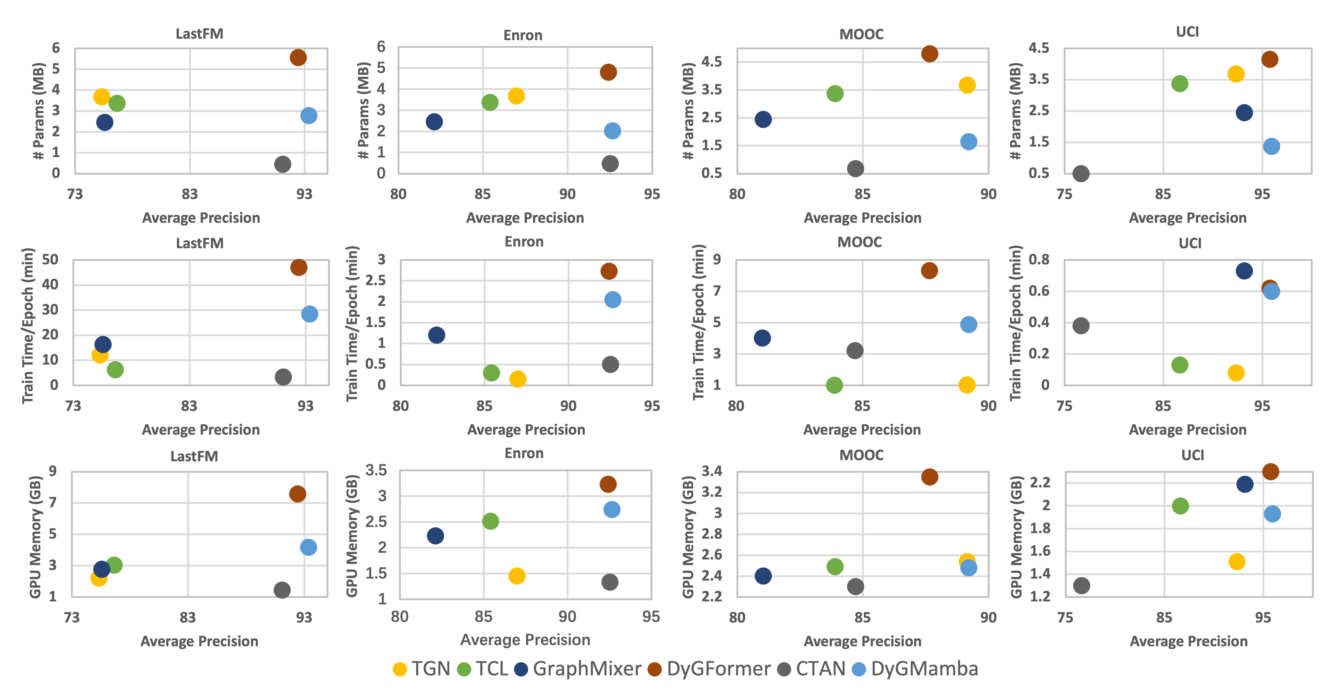
Figure 2: Efficiency comparison on four datasets among DyGMamba and five baselines in terms of number (#) of parameters, training time per epoch and GPU memory. The performance metric here is the AP of transductive link prediction under random NSS.

Model Size, Per Epoch Training Time and GPU Memory.

Fig. 2 compares DyGMamba with five baselines in terms of number of parameters (model size), per epoch training time and GPU memory consumption during training. We find that: (1) DyGMamba uses very few parameters while maintaining the best performance, showing a strong parameter efficiency. Only CTAN constantly uses fewer parameters than DyGMamba, however, its performance is much worse; (2) DyGMamba is much more efficient than DyGFormer. Note that the lengths of the sequences input into the SSM and the Transformer are the same ($\rho/p=32$), which ensures a fair comparison; (3) Although DyGMamba generally consumes more GPU memory and per epoch training time compared with most baselines, the gap of consumption is not very large in most cases. To model more temporal neighbors for long-range temporal dependent datasets, DyGMamba naturally requires more computational resources, thus enlarging the consumption gap. DyGFormer shows the same trend as DyGMamba since it also captures long-term temporal dependencies by considering more temporal neighbors; (4) CTAN requires very few computational resources. However, on long-range temporal dependent datasets, it is beaten by DyGFormer and DyGMamba with a great margin. Besides, CTAN is also hard to converge. Although it requires very little per epoch training time, it requires much more epochs to reach the best performance, leading to a long total training time. See App. H.2 and H.3 for details.

Impact of Patch Size on Scalability.

Patching treats $p$ temporal neighbors as one patch and thus decreases the sequence length by $p$ times. This is very helpful in cutting the consumption of GPU memory and training/evaluation time. However, patching introduces excessive parameters because it is done through $f_{N}$, $f_{E}$, $f_{T}$ and $f_{F}$ (Eq. 3) whose size increases as the patch size grows. Fig. 3b shows the numbers of parameters of DyGFormer and DyGmamba with different patch sizes on a long-term temporal dependent dataset Enron. We find that patching greatly affects model sizes. To further study how patching affects DyGMamba, we decrease the patch size gradually from $8$ to $1$ and track DyGMamba’s performance (Fig. 3a) as well as efficiency (Fig. 3b to 3d) on Enron. Meanwhile, we also keep track on DyGFormer under the same patch size for comparison. We have several findings: (1) Whatever the patch size is, DyGMamba always consumes fewer parameters, less GPU memory and per epoch training time, showing its high efficiency; (2) While both models require increasing computational budgets as the patch size decreases, the speed of increase is much lower for DyGMamba, demonstrating its strong scalability in modeling longer sequences; (3) Different trends in performance change are observed between two models. While DyGFormer performs worse, DyGMamba can benefit from a smaller patch size, indicating its strong ability to capture nuanced temporal details even if the sequence becomes much longer. Note that the models use fewer parameters under smaller patch size. This also shows that DyGMamba can achieve much stronger parameter efficiency by reducing patch sizes. To further study the reason for finding (3), we plot the performance of Varaint A (from ablation study A) under different patch sizes in Fig. 3a. We find that Variant A’s performance degrades when sequence length is more than $64$. This means that dynamic information selection based on edge-specific temporal patterns is essential for DyGMamba to optimally process long sequences.

(a) Enron performance.

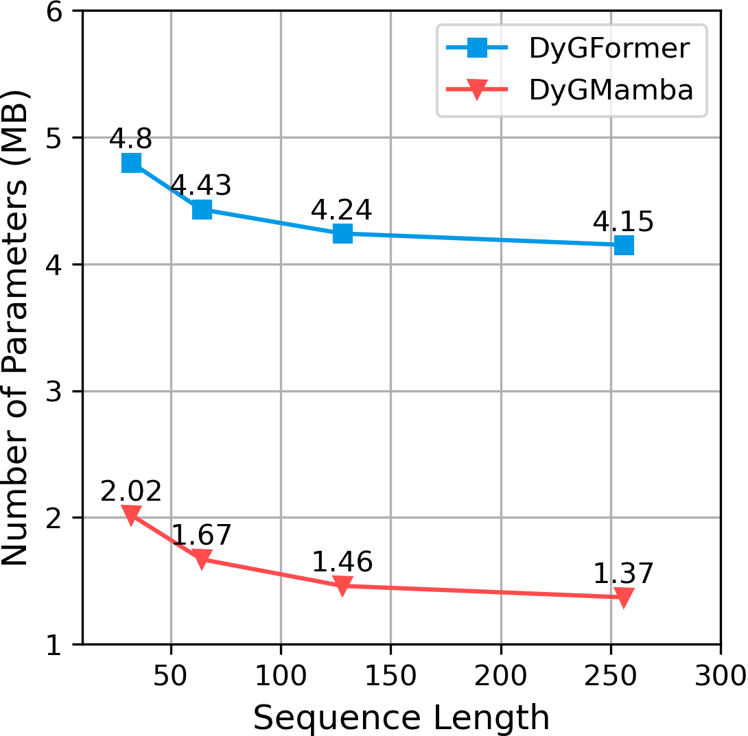
(b) Enron # params.

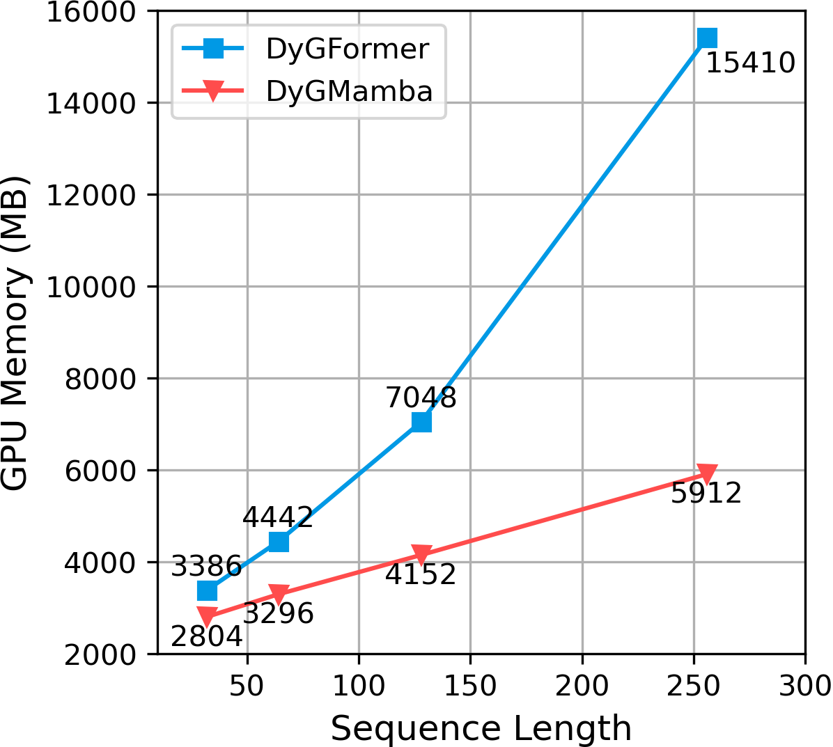
(c) Enron GPU memory.

(d) Enron train time/epoch.

Figure 3: Impact of patch size on DyGFormer, DyGMamba and Varaint A, given a fixed number of sampled temporal neighbors $\rho$ on Enron. Patch size $p$ varies from $8$, $4$, $2$, $1$. Sequence length $\rho/p$ increases as patch size decreases. Performance is the transductive AP under random NSS.

Scalability in Modeling Increasing Number of Temporal Neighbors.

Sequence length is decided by the sampled temporal neighbors $\rho$ and the patch size $p$. If we want to model a huge

Figure 4: GPU memory consumption on Enron with increasing sampled neighbors. For clarity, memory consumption is shown only when neighbors are more than $512$.

number of temporal neighbors, e.g., $\rho=4096$, keeping the sequence length unchanged as $32$ means we need to set $p$ to $128$. This will greatly increase model parameters and cause burden in parameter optimization. Besides, as shown in Fig. 3a, bigger $p$ does not necessarily lead to better performance. Therefore, it is also important to see if a model is scalable to $\rho$, with a fixed $p$. In Fig. 4, we show the consumed GPU memory of DyGMamba and DyGFormer with $\rho$ varying from $64$, $128$, $256$, $512$, $1024$, $2048$, $4096$ and $8192$ on Enron, under a fixed patch size $p=8$. We find that DyGMamba shows superior scalability over DyGFormer. While DyGFormer can only process $2048$ nodes, DyGMamba can deal with more than $8192$ (at least $4$ times) on a single 45GB NVIDIA A40 GPU. This implies our model’s potential to process a huge number of temporal neighbors with a limited GPU memory budget.

DyGMamba vs. DyGFormer on Complexity.

In historical interaction modeling, DyGMamba holds a computational complexity of $O(\rho/p)$ linear to $\rho/p$. While DyGFormer’s complexity is $O((\rho/p)^{2})$, which is quadratic to $\rho/p$. As a result, as the sequence length grows (either $\rho$ increases or $p$ decreases), DyGFormer is less scalable compared with DyGMamba. We present detailed computation and analysis of complexity in App. A.

5 Conclusion

We propose DyGMamba, an efficient CTDG representation learning model that can capture long-term temporal dependencies. DyGMamba first leverages a node-level SSM to encode long sequences of historical node interactions. It then employs a time-level SSM to learn edge-specific temporal patterns. The learned patterns are used to select the critical part of the encoded temporal information. DyGMamba achieves superior performance on dynamic link prediction, and moreover, it shows high efficiency and strong scalability compared with previous CTDG methods, implying a great potential in modeling huge amounts of temporal information with a limited computational budget.

Acknowledgement

The authors would like to thank the Federal Ministry of Education and Research and the state governments (www.nhr-verein.de/unsere-partner) for supporting this work/project as part of the joint funding of National High Performance Computing (NHR). Part of the experiments of this work was performed on the HoreKa supercomputer funded by the Ministry of Science, Research and the Arts Baden-Württemberg and by the Federal Ministry of Education and Research. This work has also been partially funded by the Munich Center for Machine Learning and supported by the Federal Ministry of Education and Research and the State of Bavaria. Zifeng Ding acknowledges travel support from the European Union’s Horizon 2020 research and innovation programme under ELISE Grant Agreement No 951847.

Appendix A Complexity Analysis between DyGMamba and DyGFormer

Given a batch size of $B$, a sequence length of $\rho/p$, a patch feature dimension size $4d$ and an SSM dimension $d_{SSM}$, we compute DyGMamba’s required computation for sequence encoding as follows. DyGMamba consists of a node-level SSM block and a time-level SSM block. For the node-level SSM block, the complexity is $O(B\cdot(\rho/p)\cdot 4d\cdot d_{SSM})$. For the time-level SSM block, the complexity is $O(B\cdot k\cdot\gamma d\cdot d_{SSM})$. Note that DyGMamba processes source and destination nodes’ sampled neighbors separately in the node-level SSM block. By considering all of these conditions, we can write DyGMamba’s complexity as $O(Bd_{SSM}d(8(\rho/p)+k\gamma))$. In practice, we choose $d_{SSM}$ as the default value of $16$. We also choose $\gamma$ as $0.5$ for all experiments. Based on this, we can further write DyGMamba’s complexity as $O(128Bd(\rho/p)+8Bdk)$. Recall that $k$ in practice is small, e.g., 10, we can thus write DyGMamba’s complexity as $O(\rho/p)$. DyGFormer concatenate source and destination nodes’ sampled neighbors into one sequence, so its complexity for sequence encoding is $O(B\cdot 4d\cdot(2\rho/p)^{2}+B\cdot(4d)^{2}\cdot(2\rho/p))=O(16Bd((\rho/p)^{2}+2\rho/p))=O((\rho/p)^{2})$. To this end, we can conclude that DyGMamba is much more scalable than DyGFormer when they are used to model long node interaction sequences.

Appendix B CTDG Dataset Details

We present the dataset statistics of all considered CTDG datasets in Table 5. All the datasets in our experiments are taken from (Yu et al., 2023). Please refer to it for detailed dataset descriptions.

Table 5: Dataset statistics. # N&E Feat means the numbers of node and edge features.

Datasets	# Nodes	# Edges	# N&E Feat	Bipartite	Duration	# Timestamps	Time Granularity
LastFM	1,980	1,293,103	0 & 0	True	1 month	1,283,614	Unix timestamps
Enron	184	125,235	0 & 0	False	3 years	22,632	Unix timestamps
MOOC	7,144	411,749	0 & 4	True	17 months	345,600	Unix timestamps
Reddit	10,984	672,447	0 & 172	True	1 month	669,065	Unix timestamps
Wikipedia	9,227	157,474	0 & 172	True	1 month	152,757	Unix timestamps
UCI	1,899	59,835	0 & 0	False	196 days	58,911	Unix timestamps
Social Evo.	74	2,099,519	0 & 2	False	8 months	565,932	Unix timestamps

Appendix C Baseline Details

We provide the detailed descriptions of all baselines here. The baselines can be split into two groups: the methods designed/not designed for long-range temporal information propagation.

C.1 Baselines Not Designed for Long-Range Temporal Information Propagation

• JODIE (Kumar et al., 2019): JODIE employs a recurrent neural network (RNN) for each node and uses a projection operation to learn the future representation trajectory of each node.

• DyRep (Trivedi et al., 2019): DyRep updates node representations as events appear. It designs a two-time scale deep temporal point process approach for source and destination nodes and couple the structural and temporal components with a temporal-attentive aggregation module.

• TGAT (Xu et al., 2020): TGAT computes the node representations by aggregating each node’s temporal neighbors based on a self-attention module. A time encoding function is proposed to learn functional representations of time.

• TGN (Rossi et al., 2020): TGN leverages an evolving memory for each node and updates the memory when a node-relevant interaction occurs by using a message function, a message aggregator, and a memory updater. An embedding module is used to generate the temporal representations of nodes.

• CAWN (Wang et al., 2021c): CAWN is a random walk-based method. It does multiple causal anonymous walks for each node and extracts relative node identities from the walk results. RNNs are then introduced to encode the anonymous walks. The aggregated walk information forms the final node representation.

• EdgeBank (Poursafaei et al., 2022): EdgeBank is a non-parametric method purely based on memory. It stores the observed interactions in its memory and updates the memory through various strategies. An interaction, i.e., link, will be predicted as existing if it is stored in the memory, and non-existing otherwise. EdgeBank uses four memory update strategies: (1) EdgeBank_∞, where all the observed edges are stored in the memory; (2) EdgeBank${}_{\text{tw-ts}}$, where only the edges within the duration of the test set from the immediate past are kept in the memory; (3) EdgeBank${}_{\text{tw-re}}$, where only the edges within the average time intervals of repeated edges from the immediate past are kept in the memory; (4) EdgeBank${}_{\text{th}}$, where the edges with appearing counts higher than a threshold are stored in the memory. The results reported in our paper correspond to the best results achieved among the four memory update strategies.

• TCL (Wang et al., 2021a): TCL first extracts temporal dependency interaction sub-graphs for source and interaction nodes and then presents a graph transformer to aggregate node information from the sub-graphs. A cross-attention operation is implemented to enable information communication between two source and destination nodes.

• GraphMixer (Cong et al., 2023): GraphMixer designs a link-encoder based on MLP-Mixer (Tolstikhin et al., 2021) to learn from the temporal interactions. A mean pooling-based node-encoder is used to aggregate the node features. Link prediction is done with a link classifier that leverages the representations output by link-encoder and node-encoder.

Note that TGN uses a memory network to store the whole graph history, making it able to preserve long-range temporal information. However, as disscussed in (Yu et al., 2023), it faces a problem of vanishing/exploding gradients, preventing it from optimally capturing long-term temporal dependencies. EdgeBank can also preserve a very long graph history, but we can observe from the experimental results (Table 1, 8) that without learnable parameters, it is not strong enough on long-range temporal dependent datasets.

C.2 Baselines Designed for Long-Range Temporal Information Propagation

• DyGFormer (Yu et al., 2023): DyGFormer is a Transformer-based CTDG model. It takes the long-term one-hop temporal interactions of source and destination nodes and use a Transformer to encode them. A patching technique is developed to cut the computational consumption and a node co-occurrence encoding scheme is used to exploit the correlations of nodes in each interaction. DyGFormer achieves long-range temporal information propagation by increasing the number of sampled one-hop historical interactions. The patching technique ensures that even with a huge number of sampled interactions, the length of the sequence input into Transformer will not be too long, making it possible to implement DyGFormer with a limited computational budget.

• CTAN (Gravina et al., 2024): CTAN is deep graph network for learning CTDGs based on non-dissipative ordinary differential equations. CTAN’s formulation allows for a scalable long-range temporal information propagation in C-TDGs because its non-dissipative layer can retain the information from a specific event indefinitely, ensuring that the historical context of a node is preserved despite the occurrence of additional events involving this node.

Appendix D Implementation Details

We train every CTDG model except for CTAN for a maximum number of $200$ epochs. Maximum epochs for CTAN training is $1000$. We evaluate each model on the validation set at the end of every training epoch and adopt an early stopping strategy with a patience of 20. We take the model that achieves the best validation result for testing. We use the implementations provided by (Yu et al., 2023) for all baseline models except CTAN. For CTAN, we use its official implementation. All models are trained with a batch size of 200 for fair efficiency analysis. All experiments are implemented with PyTorch (Paszke et al., 2019) on a server equipped with an AMD EPYC 7513 32-Core Processor and a single NVIDIA A40 with 45GB memory. We run each experiment for five times with five random seeds and report the mean results together with error bars.

D.1 Hyperparameter Configurations

For all the baselines except CTAN, please refer to (Yu et al., 2023) for the hyperparameter configurations. For CTAN, we present its hyperparameter configurations in Table 6. We keep its hyperparameters unchanged for all datasets. Note that we set the number of graph convolution layers (GCLs) in CTAN to its maximum, i.e., 5, in order to maximize its performance in capturing long-term temporal dependencies.

Table 6: Hyperparameter configurations of CTAN on all datasets. $\gamma$ here denotes the discretization step size introduced in Gravina et al. (2024), different from the one in DyGMamba.

Model	# GCL	$\epsilon$	$\gamma$	Embedding Dim
CTAN	5	0.5	0.5	128

We report the hyperparameter searching strategy of DyGMamba and the best hyperparameters in Table 7. Note that to achieve fair efficiency comparison with DyGFormer, we fix the length of the input sequence into the node-level SSM to $32$, i.e., $\rho\ \&\ p=32$. The results reported in Table 1, 2, 8, 9 are all achieved by DyGMamba with $\rho\ \&\ p=32$. In practice, we can decrease $p$ to have a better performance given more computational resources (as discussed in Sec. 4.3). DyGMamba keeps the embedding size as same as DyGFormer on all datasets, i.e., $d_{N}=d_{E}=172,d_{T}=100,d_{F}=50$. We also set $\gamma=0.5$ for all experiments of DyGMamba. The dimension of SSMs $d_{SSM}=16$ remains the default value of mamba SSM’s official repository.

Table 7: DyGMamba hyperparameter searching strategy. The best settings are marked as bold.

Dataset	Dropout	$\rho\ \&\ p$	$k$
LastFM	{0.0, 0.1, 0.2}	{1024 & 32, 512 & 16, 256 & 8}	{30, 10, 5}
Enron	{0.0, 0.1, 0.2}	{512 & 16, 256 & 8, 128 & 4}	{30, 10, 5}
MOOC	{0.0, 0.1, 0.2}	{512 & 16, 256 & 8, 128 & 4}	{30, 10, 5}
Reddit	{0.0, 0.1, 0.2}	{128 & 4, 64 & 2, 32 & 1}	{30, 10, 5}
Wikipedia	{0.0, 0.1, 0.2}	{64 & 2, 32 & 1}	{30, 10, 5}
UCI	{0.0, 0.1, 0.2}	{64 & 2, 32 & 1}	{30, 10, 5}
Social Evo.	{0.0, 0.1, 0.2}	{64 & 2, 32 & 1}	{30, 10, 5}

Appendix E Negative Edge Sampling Strategies during Evaluation

We justify why we do not do historical NSS for inductive link prediction. As described in Poursafaei et al. (2022), historical NSS focuses on sampling negative edges from the set of edges that have been observed during previous timestamps but are absent in the current step. In the setting of inductive link prediction, models are asked to predict the links between the nodes unseen in the training dataset. This means when doing historical NSS, models only need to care about the previously observed edges in the test set (or validation set during validation) for choosing negative edges. This makes historical NSS as sames as inductive NSS in the inductive link prediction, where inductive NSS samples negative edges that have been observed only in the test set, but not training set. Empirical results shown in Appendix C.2 Table 13 and 14 of Yu et al. (2023) also prove that, there is no difference between historical and inductive NSS in inductive link prediction. So we omit the results of historical NSS in our paper.

Appendix F AUC-ROC Results

Table 8 and 9 presents the AUC-ROC results of all baselines and DyGMamba. We have similar observations as the AP results shown in Table 1 and 2. DyGMamba still demonstrates superior performance and can achieve the best average rank under any NSS setting in both transductive and inductive link prediction.

Table 8: AUC-ROC of transductive dynamic link prediction.

NSS

Datasets

JODIE

DyRep

TGAT

TGN

CAWN

EdgeBank

TCL

GraphMixer

DyGFormer

CTAN

DyGMamba

Random

LastFM

70.89 $\pm$ 1.97

71.40 $\pm$ 2.12

71.47 $\pm$ 0.14

76.64 $\pm$ 4.66

85.92 $\pm$ 0.16

83.77 $\pm$ 0.00

71.09 $\pm$ 1.48

73.51 $\pm$ 0.14

93.03 $\pm$ 0.11

85.12 $\pm$ 0.77

93.31 $\pm$ 0.18

Enron

87.77 $\pm$ 2.43

83.09 $\pm$ 2.20

68.57 $\pm$ 1.46

88.72 $\pm$ 0.95

90.34 $\pm$ 0.23

87.05 $\pm$ 0.00

83.33 $\pm$ 0.93

84.16 $\pm$ 0.34

93.20 $\pm$ 0.12

87.09 $\pm$ 1.51

93.34 $\pm$ 0.23

MOOC

84.50 $\pm$ 0.60

84.50 $\pm$ 0.87

87.01 $\pm$ 0.16

91.91 $\pm$ 0.82

80.48 $\pm$ 0.41

60.86 $\pm$ 0.00

84.02 $\pm$ 0.59

84.04 $\pm$ 0.12

88.08 $\pm$ 0.50

85.40 $\pm$ 2.67

89.58 $\pm$ 0.12

Reddit

98.29 $\pm$ 0.05

98.13 $\pm$ 0.04

98.50 $\pm$ 0.01

98.61 $\pm$ 0.05

99.02 $\pm$ 0.00

95.37 $\pm$ 0.00

97.67 $\pm$ 0.01

97.17 $\pm$ 0.02

99.15 $\pm$ 0.01

97.24 $\pm$ 0.75

99.27 $\pm$ 0.01

Wikipedia

96.36 $\pm$ 0.14

94.43 $\pm$ 0.32

96.60 $\pm$ 0.07

98.37 $\pm$ 0.10

98.54 $\pm$ 0.01

90.78 $\pm$ 0.00

97.27 $\pm$ 0.06

96.89 $\pm$ 0.04

98.92 $\pm$ 0.03

97.00 $\pm$ 0.21

99.08 $\pm$ 0.02

UCI

90.35 $\pm$ 0.51

69.46 $\pm$ 2.66

78.76 $\pm$ 1.10

92.03 $\pm$ 0.69

93.81 $\pm$ 0.23

77.30 $\pm$ 0.00

85.49 $\pm$ 0.82

91.62 $\pm$ 0.52

94.45 $\pm$ 0.22

76.25 $\pm$ 2.83

94.77 $\pm$ 0.18

Social Evo.

92.13 $\pm$ 0.20

90.37 $\pm$ 0.52

94.93 $\pm$ 0.06

95.31 $\pm$ 0.27

87.34 $\pm$ 0.10

81.60 $\pm$ 0.00

95.45 $\pm$ 0.21

95.21 $\pm$ 0.07

96.25 $\pm$ 0.04

Timeout

96.38 $\pm$ 0.02

Avg. Rank

7.14

8.86

7.14

3.86

4.86

9.14

7.29

7.14

2.14

7.29

1.14

Historical

LastFM

75.65 $\pm$ 4.43

70.63 $\pm$ 2.56

64.23 $\pm$ 0.45

78.00 $\pm$ 2.97

67.92 $\pm$ 0.32

78.09 $\pm$ 0.00

60.53 $\pm$ 2.54

64.06 $\pm$ 0.34

78.80 $\pm$ 0.02

79.50 $\pm$ 0.82

79.82 $\pm$ 0.27

Enron

75.21 $\pm$ 1.27

76.36 $\pm$ 1.42

62.36 $\pm$ 1.07

76.75 $\pm$ 1.40

65.62 $\pm$ 0.49

79.59 $\pm$ 0.00

71.72 $\pm$ 1.24

74.82 $\pm$ 2.04

77.35 $\pm$ 0.64

81.95 $\pm$ 1.64

77.73 $\pm$ 0.61

MOOC

82.38 $\pm$ 1.75

80.71 $\pm$ 2.08

81.53 $\pm$ 0.79

86.59 $\pm$ 2.03

71.74 $\pm$ 0.88

61.90 $\pm$ 0.00

73.22 $\pm$ 1.21

77.09 $\pm$ 0.83

87.26 $\pm$ 0.83

73.87 $\pm$ 2.77

87.91 $\pm$ 0.93

Reddit

80.70 $\pm$ 0.20

79.96 $\pm$ 0.23

79.60 $\pm$ 0.09

81.04 $\pm$ 0.23

80.42 $\pm$ 0.20

78.58 $\pm$ 0.00

76.83 $\pm$ 0.12

77.83 $\pm$ 0.33

80.61 $\pm$ 0.48

90.63 $\pm$ 2.28

81.71 $\pm$ 0.49

Wikipedia

80.71 $\pm$ 0.64

77.49 $\pm$ 0.72

82.83 $\pm$ 0.27

83.28 $\pm$ 0.26

65.74 $\pm$ 3.46

77.27 $\pm$ 0.00

85.55 $\pm$ 0.47

87.47 $\pm$ 0.20

72.78 $\pm$ 6.65

95.43 $\pm$ 0.07

78.99 $\pm$ 1.24

UCI

78.21 $\pm$ 3.18

58.65 $\pm$ 3.58

57.12 $\pm$ 0.98

78.48 $\pm$ 1.79

57.67 $\pm$ 1.11

69.56 $\pm$ 0.00

65.42 $\pm$ 2.62

77.46 $\pm$ 1.63

75.71 $\pm$ 0.57

75.05 $\pm$ 0.13

75.43 $\pm$ 1.99

Social Evo.

91.83 $\pm$ 1.52

92.81 $\pm$ 0.60

93.63 $\pm$ 0.48

94.27 $\pm$ 1.33

87.61 $\pm$ 0.06

85.81 $\pm$ 0.00

95.03 $\pm$ 0.82

94.65 $\pm$ 0.28

97.16 $\pm$ 0.06

Timeout

97.27 $\pm$ 0.30

Avg. Rank

5.29

7.14

7.86

3.71

9.14

7.43

7.71

6.29

4.29

4.29

2.86

Inductive

LastFM

61.59 $\pm$ 5.72

60.62 $\pm$ 2.20

63.96 $\pm$ 0.41

65.48 $\pm$ 4.13

67.90 $\pm$ 0.44

77.37 $\pm$ 0.00

54.75 $\pm$ 1.31

59.98 $\pm$ 0.20

67.87 $\pm$ 0.53

78.70 $\pm$ 0.87

68.74 $\pm$ 0.55

Enron

70.75 $\pm$ 0.69

67.37 $\pm$ 2.21

59.78 $\pm$ 1.12

73.22 $\pm$ 0.42

75.29 $\pm$ 0.66

75.00 $\pm$ 0.00

69.74 $\pm$ 1.19

70.72 $\pm$ 1.08

74.67 $\pm$ 0.80

75.40 $\pm$ 1.92

75.47 $\pm$ 1.41

MOOC

67.53 $\pm$ 1.76

62.60 $\pm$ 1.27

74.44 $\pm$ 0.81

76.89 $\pm$ 2.13

70.08 $\pm$ 0.33

48.18 $\pm$ 0.00

71.80 $\pm$ 1.09

72.25 $\pm$ 0.57

80.78 $\pm$ 0.89

68.17 $\pm$ 3.73

81.08 $\pm$ 0.82

Reddit

83.40 $\pm$ 0.33

82.75 $\pm$ 0.36

87.46 $\pm$ 0.10

84.57 $\pm$ 0.19

88.19 $\pm$ 0.20

85.93 $\pm$ 0.00

84.41 $\pm$ 0.18

82.24 $\pm$ 0.24

86.25 $\pm$ 0.64

91.42 $\pm$ 2.18

86.35 $\pm$ 0.52

Wikipedia

70.41 $\pm$ 0.39

67.57 $\pm$ 0.94

81.54 $\pm$ 0.31

81.21 $\pm$ 0.30

68.48 $\pm$ 3.64

81.73 $\pm$ 0.00

73.51 $\pm$ 1.88

84.20 $\pm$ 0.36

64.09 $\pm$ 9.75

93.67 $\pm$ 0.11

75.64 $\pm$ 2.42

UCI

64.14 $\pm$ 1.25

54.10 $\pm$ 2.74

59.60 $\pm$ 0.61

63.76 $\pm$ 0.99

57.85 $\pm$ 0.59

58.03 $\pm$ 0.00

65.46 $\pm$ 2.07

74.25 $\pm$ 0.71

64.92 $\pm$ 0.83

66.51 $\pm$ 0.25

66.83 $\pm$ 2.83

Social Evo.

91.81 $\pm$ 1.69

92.77 $\pm$ 0.64

93.54 $\pm$ 0.48

94.86 $\pm$ 1.25

90.10 $\pm$ 0.11

87.88 $\pm$ 0.00

95.13 $\pm$ 0.83

94.50 $\pm$ 0.26

95.01 $\pm$ 0.15

Timeout

97.37 $\pm$ 0.26

Avg. Rank

7.86

9.57

6.14

5.43

6.29

6.43

6.71

6.00

5.14

3.86

2.57

Table 9: AUC-ROC of inductive dynamic link prediction. EdgeBank cannot do inductive link prediction so is not reported.

NSS	Datasets	JODIE	DyRep	TGAT	TGN	CAWN	TCL	GraphMixer	DyGFormer	CTAN	DyGMamba
Random	LastFM	82.49 $\pm$ 0.94	82.82 $\pm$ 1.17	76.76 $\pm$ 0.22	82.61 $\pm$ 2.62	87.92 $\pm$ 0.15	76.95 $\pm$ 1.34	80.34 $\pm$ 0.14	94.10 $\pm$ 0.09	61.49 $\pm$ 2.78	94.37 $\pm$ 0.13
	Enron	80.16 $\pm$ 1.50	75.82 $\pm$ 3.14	64.25 $\pm$ 1.29	79.40 $\pm$ 1.77	86.84 $\pm$ 0.89	81.03 $\pm$ 0.93	76.08 $\pm$ 0.92	89.59 $\pm$ 0.10	75.23 $\pm$ 2.24	89.76 $\pm$ 0.21
	MOOC	83.82 $\pm$ 0.30	83.42 $\pm$ 0.77	86.67 $\pm$ 0.24	91.58 $\pm$ 0.74	81.76 $\pm$ 0.46	82.42 $\pm$ 0.71	82.76 $\pm$ 0.13	87.75 $\pm$ 0.42	66.38 $\pm$ 1.59	89.34 $\pm$ 0.12
	Reddit	96.42 $\pm$ 0.13	95.87 $\pm$ 0.21	97.02 $\pm$ 0.04	97.30 $\pm$ 0.12	98.42 $\pm$ 0.01	94.63 $\pm$ 0.08	94.95 $\pm$ 0.08	98.70 $\pm$ 0.02	82.35 $\pm$ 4.03	98.88 $\pm$ 0.01
	Wikipedia	94.43 $\pm$ 0.28	91.31 $\pm$ 0.40	95.93 $\pm$ 0.19	97.71 $\pm$ 0.19	98.05 $\pm$ 0.03	97.03 $\pm$ 0.08	96.26 $\pm$ 0.04	98.49 $\pm$ 0.02	92.59 $\pm$ 0.70	98.72 $\pm$ 0.03
	UCI	78.78 $\pm$ 1.11	58.84 $\pm$ 2.54	77.41 $\pm$ 0.65	86.27 $\pm$ 1.49	90.27 $\pm$ 0.40	81.67 $\pm$ 1.01	89.26 $\pm$ 0.42	92.43 $\pm$ 0.20	48.58 $\pm$ 6.02	92.70 $\pm$ 0.19
	Social Evo.	93.62 $\pm$ 0.36	90.20 $\pm$ 2.05	93.52 $\pm$ 0.05	93.21 $\pm$ 0.90	84.73 $\pm$ 0.20	94.63 $\pm$ 0.06	94.09 $\pm$ 0.03	95.30 $\pm$ 0.05	Timeout	95.36 $\pm$ 0.04
	Avg. Rank	6.00	7.43	7.00	4.57	4.71	6.14	6.14	2.14	9.71	1.14
Inductive	LastFM	69.85 $\pm$ 1.70	68.14 $\pm$ 1.61	69.89 $\pm$ 0.41	67.01 $\pm$ 5.77	67.72 $\pm$ 0.20	63.15 $\pm$ 1.17	69.93 $\pm$ 0.17	69.86 $\pm$ 0.80	57.85 $\pm$ 3.67	70.59 $\pm$ 0.57
	Enron	65.95 $\pm$ 1.27	62.20 $\pm$ 2.15	56.52 $\pm$ 0.84	64.21 $\pm$ 0.94	62.07 $\pm$ 0.72	67.56 $\pm$ 1.34	67.39 $\pm$ 1.33	66.07 $\pm$ 0.65	68.70 $\pm$ 1.82	68.98 $\pm$ 1.00
	MOOC	65.37 $\pm$ 0.96	62.97 $\pm$ 2.05	74.94 $\pm$ 0.80	76.36 $\pm$ 2.91	71.18 $\pm$ 0.54	71.30 $\pm$ 1.21	72.15 $\pm$ 0.65	80.42 $\pm$ 0.72	58.06 $\pm$ 0.89	81.12 $\pm$ 0.63
	Reddit	61.84 $\pm$ 0.44	60.35 $\pm$ 0.53	64.92 $\pm$ 0.08	65.24 $\pm$ 0.08	65.37 $\pm$ 0.12	61.85 $\pm$ 0.11	64.56 $\pm$ 0.26	64.80 $\pm$ 0.53	81.70 $\pm$ 4.71	64.93 $\pm$ 0.89
	Wikipedia	61.66 $\pm$ 0.30	56.34 $\pm$ 0.67	78.40 $\pm$ 0.77	75.86 $\pm$ 0.50	59.00 $\pm$ 4.33	71.45 $\pm$ 2.23	82.76 $\pm$ 0.11	58.21 $\pm$ 8.78	91.12 $\pm$ 0.13	67.92 $\pm$ 2.23
	UCI	60.66 $\pm$ 1.82	51.50 $\pm$ 2.08	61.27 $\pm$ 0.78	62.07 $\pm$ 0.67	55.60 $\pm$ 1.22	65.87 $\pm$ 1.90	75.72 $\pm$ 0.70	64.37 $\pm$ 0.98	51.68 $\pm$ 2.60	66.95 $\pm$ 2.22
	Social Evo.	88.98 $\pm$ 0.81	86.43 $\pm$ 1.48	92.37 $\pm$ 0.50	91.66 $\pm$ 2.14	83.84 $\pm$ 0.21	95.50 $\pm$ 0.31	93.88 $\pm$ 0.22	94.97 $\pm$ 0.36	Timeout	96.65 $\pm$ 0.29
	Avg. Rank	7.00	8.71	5.14	5.14	7.14	5.14	3.57	4.71	6.14	2.29

Appendix G Dynamic Node Classification

We first give the definition of the dynamic node classification task.

Definition 3 (Dynamic Node Classification).

Given a CTDG $\mathcal{G}$, a source node $u\in\mathcal{N}$, a destination node $v\in\mathcal{N}$, a timestamp $t\in\mathcal{T}$, and all the interactions before $t$, i.e., $\{(u_{i},v_{i},t_{i})|t_{i}<t,(u_{i},v_{i},t_{i})\in\mathcal{G}\}$, dynamic node classification aims to predict the state (e.g., dynamic node label) of $u$ or $v$ at $t$ in the condition that the interaction $(u,v,t)$ exists.

We follow (Rossi et al., 2020; Xu et al., 2020; Yu et al., 2023) to conduct dynamic node classification by estimating the state of a node in a given interaction at a specific timestamp. A classification MLP is employed to map the node representations as well as the learned temporal patterns to the labels. AUC-ROC is used as the evaluation metric and we follow the dataset splits introduced in (Yu et al., 2023) ($70\%15\%/15\%$ for training/validation/testing in chronological order) for node classification. Table 10 shows the node classification results on Wikipedia and Reddit (the only two CTDG datasets for dynamic node classfication), we observe that DyGMamba can achieve the best average rank, showing its strong performance. Note that both Wikipedia and Reddit are not long-range temporal dependent datasets, therefore we do not include this part into the main body of the paper. Nonetheless, DyGMamba’s great results on these datasets further prove its strength in CTDG modeling, regardless of the type of the dataset (whether long-range temporal dependent or not).

Table 10: AUC-ROC of dynamic node classification.

Datasets	JODIE	DyRep	TGAT	TGN	CAWN	TCL	GraphMixer	DyGFormer	CTAN	DyGMamba
Wikipedia	88.10 $\pm$ 1.57	87.41 $\pm$ 1.94	83.42 $\pm$ 2.92	85.51 $\pm$ 3.28	84.59 $\pm$ 1.16	79.03 $\pm$ 1.18	85.60 $\pm$ 1.73	86.35 $\pm$ 2.19	87.38 $\pm$ 0.14	87.44 $\pm$ 0.82
Reddit	59.53 $\pm$ 3.18	63.12 $\pm$ 0.51	69.31 $\pm$ 2.18	63.21 $\pm$ 3.00	65.22 $\pm$ 0.79	68.04 $\pm$ 2.00	64.42 $\pm$ 1.15	67.67 $\pm$ 1.39	67.29 $\pm$ 0.15	67.70 $\pm$ 1.32
Avg. Rank	5.50	6.00	5.00	7.50	7.00	6.00	6.50	4.50	4.50	2.50

Appendix H Efficieny Analysis Complete Results

We first provide the efficiency analysis results of all baselines in this section. We then provide a comparison of total training time among DyGFormer, CTAN and DyGMamba.

H.1 Efficiency Statistics for all baselines

Table 11: Efficiency statistics for all baselines. EdgeBank is non-parameterized and not a machine learning model so we omit it here. # Params means number of parameters (MB). Time and Mem denote per epoch training time (min) and GPU memory (GB), respectively.

Datasets	LastFM			Enron			MOOC			UCI
Models	# Params	Time	Mem	# Params	Time	Mem	# Params	Time	Mem	# Params	Time	Mem
JODIE	0.75	4.4	2.28	0.75	0.07	1.30	0.75	0.78	2.36	0.75	0.03	1.44
DyRep	2.64	6.6	2.29	2.64	0.10	1.34	2.64	0.88	2.38	2.64	0.05	1.51
TGAT	4.02	22.75	4.15	4.02	1.28	3.46	4.02	4.08	3.64	4.02	0.60	3.42
TGN	3.68	12.14	2.21	3.68	0.15	1.45	3.68	1.03	2.54	3.68	0.08	1.51
CAWN	15.35	99.00	14.92	15.35	2.62	4.03	15.35	13.45	8.02	15.35	1.95	9.40
TCL	3.37	6.23	3.04	3.37	0.30	2.51	3.37	1.00	2.49	3.37	0.13	2.00
GraphMixer	2.45	16.35	2.78	2.45	1.20	2.23	2.45	4.02	2.40	2.45	0.73	2.19
DyGFormer	5.56	47.00	7.57	4.80	2.73	3.23	4.80	8.32	3.35	4.15	0.62	2.30
CTAN	0.45	3.33	1.44	0.47	0.50	1.33	0.68	3.22	2.30	0.50	0.38	1.30
DyGMamba	2.78	28.45	4.17	2.03	2.05	2.74	1.65	4.88	2.48	1.37	0.60	1.93

H.2 Total Training Time Comparison among DyGFormer, CTAN and DyGMamba

We present the per epoch training time, number of epochs until the best performance and the total training time in Table 12. Total training time computes the total amount of time a model requires to reach its maximum performance, without considering the patience during training. We observe that CTAN requires much more epochs to converge, e.g., on LastFM it uses almost $54$ times of epochs than DyGMamba to reach its best performance.

Table 12: Comparison among DyGFormer, CTAN and DyGMamba on per epoch training time (T${}_{\text{ep}}$ (min)), number of epochs until the best performance (# Epoch) and the total training time (T${}_{\text{tot}}$ (min)). $\text{T}_{\text{tot}}=\text{T}_{\text{ep}}\times$ # Epoch. The numbers in this table are the average results of five runs with different random seeds.

Datasets	LastFM			Enron			MOOC			UCI
Models	T${}_{\text{ep}}$	# Epoch	T${}_{\text{tot}}$	T${}_{\text{ep}}$	# Epoch	T${}_{\text{tot}}$	T${}_{\text{ep}}$	# Epoch	T${}_{\text{tot}}$	T${}_{\text{ep}}$	# Epoch	T${}_{\text{tot}}$
DyGFormer	47.00	49.60	2331.20	2.73	32.80	89.54	8.32	64.20	534.14	0.62	34.80	21.58
CTAN	3.33	635.00	2114.55	0.50	173.00	86.50	3.22	138.00	444.36	0.38	236.00	89.68
DyGMamba	28.45	11.80	335.71	2.05	33.00	67.65	4.88	38.00	185.44	0.60	28.00	16.80

H.3 Modeling an Increasing Number of Temporal Neighbors with Limited Total Training Time

Figure 5: Performance comparison among TGN, CAWN, DyGFormer, CTAN and DyGMamba on Enron, with an increasing number of encoded temporal neighbors. The metric is AP under random NSS on transductive link prediction. The time limit for training is $120$ min. If a model fails to complete training within this limit, a cross $\times$ is used to mark the data point. Dashed lines indicate that models start to exceed time limit as neighbor number increases.

To further show DyGMamba’s superior efficiency against baseline methods, we do the following experiments. We train five best performing models (as shown in Table 1) on Enron with a gradually increasing number of temporal neighbors and report their performance. The number of sampled neighbors spans from $8$, $16$, $32$, $64$, $128$ to $256$ (Note that these numbers are different from the best hyperparamters reported in (Yu et al., 2023)). We fix the patch size $p$ of DyGFormer and DyGMamba to $1$ in order to maximize their input sequence lengths. We set a time limit of $120$ minutes for the total training time. We let all the experiments finish the complete training process and note down the ones that exceed the time limit. In this way, we not only care about the per epoch training time, but also pay attention to how long it takes for models to converge. The experimental results are reported in Fig. 5. The points marked with crosses ($\times$) mean that the training process cannot finish within the time limit (although we still plot their corresponding performance). We find that only TGN and DyGMamba can successfully converge within the time limit when the number of considered neighbors increases to $256$. DyGMamba can constantly achieve performance gain from modeling more temporal neighbors while TGN cannot. CAWN is extremely time consuming so it cannot finish training within the time limit even when it is asked to model $16$ temporal neighbors. As for the methods designed for long-range temporal information propagation, DyGFormer and CTAN consume much longer total training time than DyGMamba. They fail to converge within $120$ minutes when the number of considered neighbors reaches $128$ and $256$, respectively. We also observe that CTAN’s performance fluctuates greatly with the increasing temporal neighbors, indicating that it is not stable to model a large number of temporal neighbors. This also implies that increasing the amount of historical information will gradually make CTAN harder to converge, which might cause trouble in modeling long range temporal dependent datasets.

References

- Behrouz & Hashemi (2024) Ali Behrouz and Farnoosh Hashemi. Graph mamba: Towards learning on graphs with state space models. CoRR, abs/2402.08678, 2024. doi: 10.48550/ARXIV.2402.08678. URL https://doi.org/10.48550/arXiv.2402.08678.
- Besta et al. (2023) Maciej Besta, Afonso Claudino Catarino, Lukas Gianinazzi, Nils Blach, Piotr Nyczyk, Hubert Niewiadomski, and Torsten Hoefler. HOT: higher-order dynamic graph representation learning with efficient transformers. In Soledad Villar and Benjamin Chamberlain (eds.), Learning on Graphs Conference, 27-30 November 2023, Virtual Event, volume 231 of Proceedings of Machine Learning Research, pp. 15. PMLR, 2023. URL https://proceedings.mlr.press/v231/besta24a.html.
- Chang et al. (2020) Xiaofu Chang, Xuqin Liu, Jianfeng Wen, Shuang Li, Yanming Fang, Le Song, and Yuan Qi. Continuous-time dynamic graph learning via neural interaction processes. In Mathieu d’Aquin, Stefan Dietze, Claudia Hauff, Edward Curry, and Philippe Cudré-Mauroux (eds.), CIKM ’20: The 29th ACM International Conference on Information and Knowledge Management, Virtual Event, Ireland, October 19-23, 2020, pp. 145–154. ACM, 2020. doi: 10.1145/3340531.3411946. URL https://doi.org/10.1145/3340531.3411946.
- Cong et al. (2023) Weilin Cong, Si Zhang, Jian Kang, Baichuan Yuan, Hao Wu, Xin Zhou, Hanghang Tong, and Mehrdad Mahdavi. Do we really need complicated model architectures for temporal networks? In The Eleventh International Conference on Learning Representations, ICLR 2023, Kigali, Rwanda, May 1-5, 2023. OpenReview.net, 2023. URL https://openreview.net/pdf?id=ayPPc0SyLv1.
- Duman Keles et al. (2023) Feyza Duman Keles, Pruthuvi Mahesakya Wijewardena, and Chinmay Hegde. On the computational complexity of self-attention. In Shipra Agrawal and Francesco Orabona (eds.), Proceedings of The 34th International Conference on Algorithmic Learning Theory, volume 201 of Proceedings of Machine Learning Research, pp. 597–619. PMLR, 20 Feb–23 Feb 2023. URL https://proceedings.mlr.press/v201/duman-keles23a.html.
- Goyal et al. (2020) Palash Goyal, Sujit Rokka Chhetri, and Arquimedes Canedo. dyngraph2vec: Capturing network dynamics using dynamic graph representation learning. Knowl. Based Syst., 187, 2020. doi: 10.1016/J.KNOSYS.2019.06.024. URL https://doi.org/10.1016/j.knosys.2019.06.024.
- Gravina et al. (2024) Alessio Gravina, Giulio Lovisotto, Claudio Gallicchio, Davide Bacciu, and Claas Grohnfeldt. Long range propagation on continuous-time dynamic graphs. In Forty-first International Conference on Machine Learning, 2024. URL https://openreview.net/forum?id=gVg8V9isul.
- Gu & Dao (2023) Albert Gu and Tri Dao. Mamba: Linear-time sequence modeling with selective state spaces. CoRR, abs/2312.00752, 2023. doi: 10.48550/ARXIV.2312.00752. URL https://doi.org/10.48550/arXiv.2312.00752.
- Gu et al. (2021) Albert Gu, Isys Johnson, Karan Goel, Khaled Saab, Tri Dao, Atri Rudra, and Christopher Ré. Combining recurrent, convolutional, and continuous-time models with linear state space layers. In Marc’Aurelio Ranzato, Alina Beygelzimer, Yann N. Dauphin, Percy Liang, and Jennifer Wortman Vaughan (eds.), Advances in Neural Information Processing Systems 34: Annual Conference on Neural Information Processing Systems 2021, NeurIPS 2021, December 6-14, 2021, virtual, pp. 572–585, 2021. URL https://proceedings.neurips.cc/paper/2021/hash/05546b0e38ab9175cd905eebcc6ebb76-Abstract.html.
- Gu et al. (2022a) Albert Gu, Karan Goel, Ankit Gupta, and Christopher Ré. On the parameterization and initialization of diagonal state space models. In Sanmi Koyejo, S. Mohamed, A. Agarwal, Danielle Belgrave, K. Cho, and A. Oh (eds.), Advances in Neural Information Processing Systems 35: Annual Conference on Neural Information Processing Systems 2022, NeurIPS 2022, New Orleans, LA, USA, November 28 - December 9, 2022, 2022a. URL http://papers.nips.cc/paper_files/paper/2022/hash/e9a32fade47b906de908431991440f7c-Abstract-Conference.html.
- Gu et al. (2022b) Albert Gu, Karan Goel, and Christopher Ré. Efficiently modeling long sequences with structured state spaces. In The Tenth International Conference on Learning Representations, ICLR 2022, Virtual Event, April 25-29, 2022. OpenReview.net, 2022b. URL https://openreview.net/forum?id=uYLFoz1vlAC.
- Huo et al. (2018) Zepeng Huo, Xiao Huang, and Xia Hu. Link prediction with personalized social influence. In Sheila A. McIlraith and Kilian Q. Weinberger (eds.), Proceedings of the Thirty-Second AAAI Conference on Artificial Intelligence, (AAAI-18), the 30th innovative Applications of Artificial Intelligence (IAAI-18), and the 8th AAAI Symposium on Educational Advances in Artificial Intelligence (EAAI-18), New Orleans, Louisiana, USA, February 2-7, 2018, pp. 2289–2296. AAAI Press, 2018. doi: 10.1609/AAAI.V32I1.11892. URL https://doi.org/10.1609/aaai.v32i1.11892.
- Jin et al. (2022) Ming Jin, Yuan-Fang Li, and Shirui Pan. Neural temporal walks: Motif-aware representation learning on continuous-time dynamic graphs. In Sanmi Koyejo, S. Mohamed, A. Agarwal, Danielle Belgrave, K. Cho, and A. Oh (eds.), Advances in Neural Information Processing Systems 35: Annual Conference on Neural Information Processing Systems 2022, NeurIPS 2022, New Orleans, LA, USA, November 28 - December 9, 2022, 2022. URL http://papers.nips.cc/paper_files/paper/2022/hash/7dadc855cef7494d5d956a8d28add871-Abstract-Conference.html.
- Kazemi et al. (2020) Seyed Mehran Kazemi, Rishab Goel, Kshitij Jain, Ivan Kobyzev, Akshay Sethi, Peter Forsyth, and Pascal Poupart. Representation learning for dynamic graphs: A survey. J. Mach. Learn. Res., 21:70:1–70:73, 2020. URL http://jmlr.org/papers/v21/19-447.html.
- Kumar et al. (2019) Srijan Kumar, Xikun Zhang, and Jure Leskovec. Predicting dynamic embedding trajectory in temporal interaction networks. In Ankur Teredesai, Vipin Kumar, Ying Li, Rómer Rosales, Evimaria Terzi, and George Karypis (eds.), Proceedings of the 25th ACM SIGKDD International Conference on Knowledge Discovery & Data Mining, KDD 2019, Anchorage, AK, USA, August 4-8, 2019, pp. 1269–1278. ACM, 2019. doi: 10.1145/3292500.3330895. URL https://doi.org/10.1145/3292500.3330895.
- Li et al. (2024) Jintang Li, Ruofan Wu, Xinzhou Jin, Boqun Ma, Liang Chen, and Zibin Zheng. State space models on temporal graphs: A first-principles study. arXiv preprint arXiv:2406.00943, 2024.
- Liu et al. (2022) Yunyu Liu, Jianzhu Ma, and Pan Li. Neural predicting higher-order patterns in temporal networks. In Frédérique Laforest, Raphaël Troncy, Elena Simperl, Deepak Agarwal, Aristides Gionis, Ivan Herman, and Lionel Médini (eds.), WWW ’22: The ACM Web Conference 2022, Virtual Event, Lyon, France, April 25 - 29, 2022, pp. 1340–1351. ACM, 2022. doi: 10.1145/3485447.3512181. URL https://doi.org/10.1145/3485447.3512181.
- Ma et al. (2023) Xuezhe Ma, Chunting Zhou, Xiang Kong, Junxian He, Liangke Gui, Graham Neubig, Jonathan May, and Luke Zettlemoyer. Mega: Moving average equipped gated attention. In The Eleventh International Conference on Learning Representations, ICLR 2023, Kigali, Rwanda, May 1-5, 2023. OpenReview.net, 2023. URL https://openreview.net/pdf?id=qNLe3iq2El.
- Ma et al. (2020) Yao Ma, Ziyi Guo, Zhaochun Ren, Jiliang Tang, and Dawei Yin. Streaming graph neural networks. In Jimmy X. Huang, Yi Chang, Xueqi Cheng, Jaap Kamps, Vanessa Murdock, Ji-Rong Wen, and Yiqun Liu (eds.), Proceedings of the 43rd International ACM SIGIR conference on research and development in Information Retrieval, SIGIR 2020, Virtual Event, China, July 25-30, 2020, pp. 719–728. ACM, 2020. doi: 10.1145/3397271.3401092. URL https://doi.org/10.1145/3397271.3401092.
- Pareja et al. (2020) Aldo Pareja, Giacomo Domeniconi, Jie Chen, Tengfei Ma, Toyotaro Suzumura, Hiroki Kanezashi, Tim Kaler, Tao B. Schardl, and Charles E. Leiserson. Evolvegcn: Evolving graph convolutional networks for dynamic graphs. In The Thirty-Fourth AAAI Conference on Artificial Intelligence, AAAI 2020, The Thirty-Second Innovative Applications of Artificial Intelligence Conference, IAAI 2020, The Tenth AAAI Symposium on Educational Advances in Artificial Intelligence, EAAI 2020, New York, NY, USA, February 7-12, 2020, pp. 5363–5370. AAAI Press, 2020. doi: 10.1609/AAAI.V34I04.5984. URL https://doi.org/10.1609/aaai.v34i04.5984.
- Paszke et al. (2019) Adam Paszke, Sam Gross, Francisco Massa, Adam Lerer, James Bradbury, Gregory Chanan, Trevor Killeen, Zeming Lin, Natalia Gimelshein, Luca Antiga, Alban Desmaison, Andreas Köpf, Edward Z. Yang, Zachary DeVito, Martin Raison, Alykhan Tejani, Sasank Chilamkurthy, Benoit Steiner, Lu Fang, Junjie Bai, and Soumith Chintala. Pytorch: An imperative style, high-performance deep learning library. In Hanna M. Wallach, Hugo Larochelle, Alina Beygelzimer, Florence d’Alché-Buc, Emily B. Fox, and Roman Garnett (eds.), Advances in Neural Information Processing Systems 32: Annual Conference on Neural Information Processing Systems 2019, NeurIPS 2019, December 8-14, 2019, Vancouver, BC, Canada, pp. 8024–8035, 2019. URL https://proceedings.neurips.cc/paper/2019/hash/bdbca288fee7f92f2bfa9f7012727740-Abstract.html.
- Peng et al. (2023) Bo Peng, Eric Alcaide, Quentin Anthony, Alon Albalak, Samuel Arcadinho, Stella Biderman, Huanqi Cao, Xin Cheng, Michael Chung, Leon Derczynski, Xingjian Du, Matteo Grella, Kranthi Kiran GV, Xuzheng He, Haowen Hou, Przemyslaw Kazienko, Jan Kocon, Jiaming Kong, Bartlomiej Koptyra, Hayden Lau, Jiaju Lin, Krishna Sri Ipsit Mantri, Ferdinand Mom, Atsushi Saito, Guangyu Song, Xiangru Tang, Johan S. Wind, Stanislaw Wozniak, Zhenyuan Zhang, Qinghua Zhou, Jian Zhu, and Rui-Jie Zhu. RWKV: reinventing rnns for the transformer era. In Houda Bouamor, Juan Pino, and Kalika Bali (eds.), Findings of the Association for Computational Linguistics: EMNLP 2023, Singapore, December 6-10, 2023, pp. 14048–14077. Association for Computational Linguistics, 2023. doi: 10.18653/V1/2023.FINDINGS-EMNLP.936. URL https://doi.org/10.18653/v1/2023.findings-emnlp.936.
- Petrović et al. (2024) Katarina Petrović, Shenyang Huang, Farimah Poursafaei, and Petar Veličković. Temporal graph rewiring with expander graphs. arXiv preprint arXiv:2406.02362, 2024.
- Poursafaei et al. (2022) Farimah Poursafaei, Shenyang Huang, Kellin Pelrine, and Reihaneh Rabbany. Towards better evaluation for dynamic link prediction. In Sanmi Koyejo, S. Mohamed, A. Agarwal, Danielle Belgrave, K. Cho, and A. Oh (eds.), Advances in Neural Information Processing Systems 35: Annual Conference on Neural Information Processing Systems 2022, NeurIPS 2022, New Orleans, LA, USA, November 28 - December 9, 2022, 2022. URL http://papers.nips.cc/paper_files/paper/2022/hash/d49042a5d49818711c401d34172f9900-Abstract-Datasets_and_Benchmarks.html.
- Rossi et al. (2020) Emanuele Rossi, Ben Chamberlain, Fabrizio Frasca, Davide Eynard, Federico Monti, and Michael M. Bronstein. Temporal graph networks for deep learning on dynamic graphs. CoRR, abs/2006.10637, 2020. URL https://arxiv.org/abs/2006.10637.
- Sankar et al. (2020) Aravind Sankar, Yanhong Wu, Liang Gou, Wei Zhang, and Hao Yang. Dysat: Deep neural representation learning on dynamic graphs via self-attention networks. In James Caverlee, Xia (Ben) Hu, Mounia Lalmas, and Wei Wang (eds.), WSDM ’20: The Thirteenth ACM International Conference on Web Search and Data Mining, Houston, TX, USA, February 3-7, 2020, pp. 519–527. ACM, 2020. doi: 10.1145/3336191.3371845. URL https://doi.org/10.1145/3336191.3371845.
- Smith et al. (2023) Jimmy T. H. Smith, Andrew Warrington, and Scott W. Linderman. Simplified state space layers for sequence modeling. In The Eleventh International Conference on Learning Representations, ICLR 2023, Kigali, Rwanda, May 1-5, 2023. OpenReview.net, 2023. URL https://openreview.net/pdf?id=Ai8Hw3AXqks.
- Tian et al. (2024) Yuxing Tian, Yiyan Qi, and Fan Guo. Freedyg: Frequency enhanced continuous-time dynamic graph model for link prediction. In The Twelfth International Conference on Learning Representations, 2024. URL https://openreview.net/forum?id=82Mc5ilInM.
- Tolstikhin et al. (2021) Ilya O. Tolstikhin, Neil Houlsby, Alexander Kolesnikov, Lucas Beyer, Xiaohua Zhai, Thomas Unterthiner, Jessica Yung, Andreas Steiner, Daniel Keysers, Jakob Uszkoreit, Mario Lucic, and Alexey Dosovitskiy. Mlp-mixer: An all-mlp architecture for vision. In Marc’Aurelio Ranzato, Alina Beygelzimer, Yann N. Dauphin, Percy Liang, and Jennifer Wortman Vaughan (eds.), Advances in Neural Information Processing Systems 34: Annual Conference on Neural Information Processing Systems 2021, NeurIPS 2021, December 6-14, 2021, virtual, pp. 24261–24272, 2021. URL https://proceedings.neurips.cc/paper/2021/hash/cba0a4ee5ccd02fda0fe3f9a3e7b89fe-Abstract.html.
- Trivedi et al. (2019) Rakshit Trivedi, Mehrdad Farajtabar, Prasenjeet Biswal, and Hongyuan Zha. Dyrep: Learning representations over dynamic graphs. In 7th International Conference on Learning Representations, ICLR 2019, New Orleans, LA, USA, May 6-9, 2019. OpenReview.net, 2019. URL https://openreview.net/forum?id=HyePrhR5KX.
- Vaswani et al. (2017) Ashish Vaswani, Noam Shazeer, Niki Parmar, Jakob Uszkoreit, Llion Jones, Aidan N. Gomez, Lukasz Kaiser, and Illia Polosukhin. Attention is all you need. In Isabelle Guyon, Ulrike von Luxburg, Samy Bengio, Hanna M. Wallach, Rob Fergus, S. V. N. Vishwanathan, and Roman Garnett (eds.), Advances in Neural Information Processing Systems 30: Annual Conference on Neural Information Processing Systems 2017, December 4-9, 2017, Long Beach, CA, USA, pp. 5998–6008, 2017. URL https://proceedings.neurips.cc/paper/2017/hash/3f5ee243547dee91fbd053c1c4a845aa-Abstract.html.
- Wang et al. (2024) Chloe Wang, Oleksii Tsepa, Jun Ma, and Bo Wang. Graph-mamba: Towards long-range graph sequence modeling with selective state spaces. CoRR, abs/2402.00789, 2024. doi: 10.48550/ARXIV.2402.00789. URL https://doi.org/10.48550/arXiv.2402.00789.
- Wang et al. (2021a) Lu Wang, Xiaofu Chang, Shuang Li, Yunfei Chu, Hui Li, Wei Zhang, Xiaofeng He, Le Song, Jingren Zhou, and Hongxia Yang. TCL: transformer-based dynamic graph modelling via contrastive learning. CoRR, abs/2105.07944, 2021a. URL https://arxiv.org/abs/2105.07944.
- Wang et al. (2023) Wen Wang, Wei Zhang, Shukai Liu, Qi Liu, Bo Zhang, Leyu Lin, and Hongyuan Zha. Incorporating link prediction into multi-relational item graph modeling for session-based recommendation. IEEE Trans. Knowl. Data Eng., 35(3):2683–2696, 2023. doi: 10.1109/TKDE.2021.3111436. URL https://doi.org/10.1109/TKDE.2021.3111436.
- Wang et al. (2021b) Xuhong Wang, Ding Lyu, Mengjian Li, Yang Xia, Qi Yang, Xinwen Wang, Xinguang Wang, Ping Cui, Yupu Yang, Bowen Sun, and Zhenyu Guo. APAN: asynchronous propagation attention network for real-time temporal graph embedding. In Guoliang Li, Zhanhuai Li, Stratos Idreos, and Divesh Srivastava (eds.), SIGMOD ’21: International Conference on Management of Data, Virtual Event, China, June 20-25, 2021, pp. 2628–2638. ACM, 2021b. doi: 10.1145/3448016.3457564. URL https://doi.org/10.1145/3448016.3457564.
- Wang et al. (2021c) Yanbang Wang, Yen-Yu Chang, Yunyu Liu, Jure Leskovec, and Pan Li. Inductive representation learning in temporal networks via causal anonymous walks. In 9th International Conference on Learning Representations, ICLR 2021, Virtual Event, Austria, May 3-7, 2021. OpenReview.net, 2021c. URL https://openreview.net/forum?id=KYPz4YsCPj.
- Xu et al. (2020) Da Xu, Chuanwei Ruan, Evren Körpeoglu, Sushant Kumar, and Kannan Achan. Inductive representation learning on temporal graphs. In 8th International Conference on Learning Representations, ICLR 2020, Addis Ababa, Ethiopia, April 26-30, 2020. OpenReview.net, 2020. URL https://openreview.net/forum?id=rJeW1yHYwH.
- You et al. (2022) Jiaxuan You, Tianyu Du, and Jure Leskovec. ROLAND: graph learning framework for dynamic graphs. In Aidong Zhang and Huzefa Rangwala (eds.), KDD ’22: The 28th ACM SIGKDD Conference on Knowledge Discovery and Data Mining, Washington, DC, USA, August 14 - 18, 2022, pp. 2358–2366. ACM, 2022. doi: 10.1145/3534678.3539300. URL https://doi.org/10.1145/3534678.3539300.
- Yu et al. (2023) Le Yu, Leilei Sun, Bowen Du, and Weifeng Lv. Towards better dynamic graph learning: New architecture and unified library. In Alice Oh, Tristan Naumann, Amir Globerson, Kate Saenko, Moritz Hardt, and Sergey Levine (eds.), Advances in Neural Information Processing Systems 36: Annual Conference on Neural Information Processing Systems 2023, NeurIPS 2023, New Orleans, LA, USA, December 10 - 16, 2023, 2023. URL http://papers.nips.cc/paper_files/paper/2023/hash/d611019afba70d547bd595e8a4158f55-Abstract-Conference.html.