A New Approach for Calculation of Quasi-Normal Modes and Topological Charges of Regular Black Holes
Abstract
This study examines the properties of a special regular black hole. This analysis investigates the Hawking temperature, remnant radius and mass, as well as the effect of parameter on thermodynamic quantities like entropy, heat capacity, and free energy. The emission rate, evaporation process, quasi-normal modes by calculating Rosen-Morse potential, and topological behavior of the black hole are also explored.
Keywords: Regular black holes, topological charge, thermodynamic properties
I Introduction
The standard cosmological model has been highly successful in describing the large-scale structure and evolution of the universe. However, there are some outstanding issues that are not well explained by this model. Therefore, alternative theories, such as modified gravity have been proposed to address these problems Clifton ; Shankaranarayanan ; Capozziello ; Bonanno . These modified gravity theories postulate the existence of additional fields or modifications to the gravitational sector, which can lead to predictions and observational signatures that differ from the standard model Nojiri ; Ashtekar .
The authors in Ref. Bonanno presented a theoretical model for the collapse of dust in the concept of asymptotically safe gravity. They introduced a function that is derived from the Reuter fixed point in asymptotically safe gravity and investigated the coupling of the matter Lagrangian and the gravitational sector. In this way, the gravitational coupling vanishes at high energies, preventing the formation of singularities during the collapse of dust. The introduced metric is given by
| (1) |
where and are given by
| (2) | ||||
| (3) |
When parameter tends to zero, metric reduces to the Schwarzschild black hole.
In Ref. Stashko , the author investigated some features of this metric such as shadow radius, quasi-normal modes by Chebyshev pseudo-spectral and Eikonal approaches, and greybody bounds.
In this work, we first provide an introduction, and then in Sec. II, we investigate the Hawking temperature, remnant mass, and radius. In Sec. III, we calculate some thermodynamic properties of the black hole, namely the entropy, heat capacity, and free energy. Subsequently, considering the shadow radius and the remnant radius, in Sec. IV we calculate the emission rate and the evaporation time of the black hole. We also calculate the quasi-normal modes for the expanded form of the metric using the Rosen-Morse potential in Sec. V. In Sec. VI and VII, we calculate the topological phase transition for several different vector potentials and their topological charge. Finally, in Sec. VIII, we present the summary and conclusion of the work.
II Remnant Radius and Mass
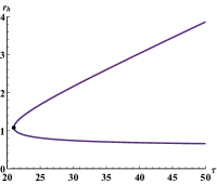
As author discussed in Ref. Stashko , three regimes which bounds parameter are existed. Case which consists of two horizon (inner and outer) radii, case that two horizon radii coincides to a single horizon and case which is horizonless. In this work we choose the first regime where . At horizon , thus one can find mass as a function of
| (4) |
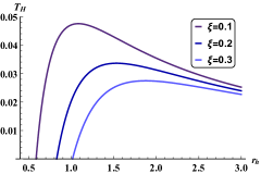
Hawking temperature of the black hole is obtained from
| (5) |
Replacing mass from Eq, (4) in Eq. (5) yields
| (6) |
III Entropy, Heat Capacity, Free Energy
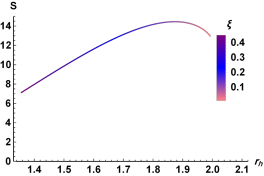
Black hole entropy is given by remnant
| (9) |
where Ei represents the exponential integral function. When tends zero, entropy becomes . The illustration of entropy versus parameter is shown in Fig. 2, where is calculated by varying parameter .
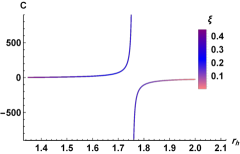
Evidently, for larger , heat capacity becomes positive, at a phase transition occurs and heat capacity takes a negative sign. As known, a black hole system exhibiting a positive specific heat capacity is indicative of thermodynamic stability, because it necessitates the injection of energy to drive an increase in temperature. Conversely, a negative specific heat capacity referred to thermodynamic instability, where the black hole cools down despite absorbing energy, which indicates its peculiar thermal response.
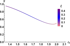
Helmholtz free energy of the system is given by
| (11) |
Fig. 4 represents the free energy curve as a function of horizon radius.
IV Emission Rate, Evaporation Time
Photon radius of the black hole is calculated from Claudel ; Virbhadra
| (12) |
and is given by Stashko
| (13) |
Shadow radius is given by
| (14) |
On the other hand, emission rate has the following from Cardoso ; Das ; emissionWei
| (15) |
where represents the cross section and is given by
| (16) |
By substituting Eqs. (14) and (16), in Eq. (15), the emission rate could be find. In Fig. 5, the demonstration of emission rate for three different is shown.
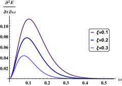
As can be seen, decreasing parameter lowered the maximum value of emission rate and causes this maximum occur in a smaller value of .
Lifetime of a black hole could be found as remnant ; evaporation2
| (17) |
where represents the product of greybody factor and the radiation constant. Here we assume . Thus
| (18) |
In case of , life time of the black hole becomes , by increasing parameter to , evaporation time yields , and choosing parameter as , evaporation time becomes as order of .
V Rosen-Morse Potential and Quasi-Normal Modes
Quasi-normal modes are characteristic oscillations of perturbed black holes, which arise from the interaction of the black hole with its surrounding. These modes provide insights into the astrophysical properties of black holes and have applications in fields like string theory, brane-world models, and the study of quark-gluon plasmas Konoplya2 ; Pedrotti .
Author in Ref. Stashko , reported the quasi-normal modes of metric (2) for scalar, vector and Dirac fields using Chebyshev pseudo-spectral and Eikonal methods. In this section, quasi-normal modes of the black hole using Rosen-Morse potential for the expanded form of metric.
By expanding logarithm function, metric (2) yields to
| (19) |
The effective potential is obtained from by Konoplya
| (20) |
where parameter represents the angular momentum and indicates the shape of perturbation. Case represents scalar perturbation and case expresses electromagnetic perturbation.
In tortoise coordinate Konoplya ; Heidari
| (21) |
Rosen-Morse function Rosen ; Heidari2
| (22) |
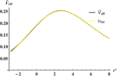
Here we chose metric of form Eq. (19). By fitting potential of to the curve, parameters of RM potential and can be find. Fig. 6 shows the fitted Rosen-Morse potential (dashed yellow curve)to the effective potential (purple curve) for and .
Quasi-normal of Rosen-Morse potential are obtained from Heidari2
| (23) |
In this case we used to approximation, the first one in expanding logarithm function, and the second one in fitting potential curve. However the mean absolute error of fitting in our work, for case , is as order of . The quasi-normal modes of metric (19), using Rosen-Morse approach for cases and are reported in table 1.
| QNMs | QNMs | ||
|---|---|---|---|
VI Topological Charge
In order to investigate the topology of a black hole, one can assume a potential function in polar coordinate related to the metric (1) as TopoCharge ; Cunha
| (24) |
Using potential, a vector field can be defined as Cunha
| (25a) | |||
| (25b) |
for and which are defined in Eqs. (2) and (3), Eqs. (25a) and (25b) yields to
| (26a) | ||||
| (26b) |
The normalized form of the above vectors can be found from
| (27) |
where index indicates the shape of potential field. The presentation of vector space is used to illustrate the topological phase transition. The intersection of vectors with opposite directions indicates a phase transition. Each topological phase transition can be assigned a topological charge, which is calculated in the following.
Deflection angle of the topological charge is given by TopoCharge ; TopoDr
| (28) |
thus
| (29) |
Using Eqs. (24) and (29), one can see that has one or more poles which are located at , and which is the solution(s) of Eq. (12).
In order to release the singularity, the following variables are used TopoCharge
| (30) |
Thus the topological charge, called winding number, is obtained from
| (31) |
Parameter takes , that the values indicate the phase transition, and the value indicates no phase change in the black hole. The whole charge is calculated from the summation of all s.
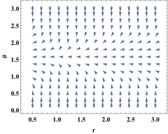
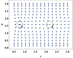
Fig. 7 demonstrates the vector space of , when parameters are set as and .
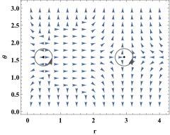
As evident, two topological charge existed and the whole charge is .
VII Temperature and Free Energy Phase Transitions
Another field can be written in the following form TopoTempWei ; TopoDr3
| (32) |
that indicates the Hawking temperature. Relevant vectors of the field (32) are defined as
| (33a) | ||||
| (33b) |
by using Eq. 6, vectors yield to
| (34a) | ||||
| (34b) |
As mentioned in Eq. (27), the normalized form of this vectors can be write.
The illustration of for the case , is shown in Fig. 8.
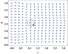
Obviously, one topological charge exists in this field and the whole charge is .
Free energy of the black hole is obtained in Eq. (III). Using the definition , Eq. (III) is rewritten as TopoEnergyWei ; TopoDr2
| (35) |
Considering as another field potential, vector space of this field are given by
| (36a) | ||||
| (36b) |
Applying from Eq. (35), to (36a), vectors of the relevant field are rewritten as
| (37) |
At , can be find as a function of . The illustration of where parameter is chose as , is shown in Fig. 9.
As obvious in Fig. 9, in case of , the critical value of is located at , and we expect different behavior of Helmholtz free energy field on both side of . Thus, vector space of this field in case of in both regime of , and is shown in Figs. 10(a) and 10(b), respectively.
As expected, in , free energy potential field phases causes two topological charge, while in case of , there is no topological charge. However in both cases the whole charge is .
VIII Conclusion
In this work, we have investigated some properties of regular black holes. In the first step, by examining the Hawking temperature of the metric , we identified that an increase in the parameter leads to an increase in the temperature of the black hole. We also calculated the remnant radius and remnant mass of the black hole. In the further investigation of the black hole, we saw how changes in the parameter affect the entropy, heat capacity, and free energy of the black hole. We studied the emission rate and the evaporation process of the black hole for different values of . We then expanded the metric and calculated the quasi-normal modes for this metric and observed the effect of changing the parameter . In the final step, we investigated the topological behavior of the black hole due to different vector fields and calculated the topological charge for the relevant fields.
Acknowledgements
The research was partially supported by the Long-Term Conceptual Development of a University of Hradec Králové for 2023, issued by the Ministry of Education, Youth, and Sports of the Czech Republic.
References
- [1]