Reconciling Early and Late Time Tensions with Reinforcement Learning

Abstract

We study the possibility of accommodating both early and late-time tensions using a novel reinforcement learning technique. By applying this technique, we aim to optimize the evolution of the Hubble parameter from recombination to the present epoch, addressing both tensions simultaneously. To maximize the goodness of fit, our learning technique achieves a fit that surpasses even the $\Lambda$CDM model. Our results demonstrate a tendency to weaken both early and late time tensions in a completely model-independent manner.

1 Introduction

The recent cosmological observations related to the expansion of the universe and structure formation have posed significant challenges to the widely accepted $\Lambda$CDM model, which has long been considered the best candidate for explaining the universe at large scales [1, 2, 3]. The $\Lambda$CDM model, along with models that mimic it by incorporating scalar degrees of freedom, is increasingly coming under scrutiny [4, 5]. These models often fall short of meeting the requirements set by recent observational data, making it a serious challenge to identify which model best explains various observations of the universe. Despite extensive theoretical efforts, a definitive answer remains elusive. However, the advent of machine learning (ML) offers a promising avenue to explore. In particular, it can help us to identify the most plausible dynamics of the universe that align more closely with observations than the $\Lambda$CDM model.

Several observations, including SH0ES [6, 7], JWST [10], and the latest DESI [11], have prompted the exploration of alternate cosmological models as they strongly disfavor the $\Lambda$CDM model:

• SH0ES (Supernovae $H0$ for the Equation of State): It directly measures the Hubble constant value using SN1a (Supernovae type 1a) calibrated with Cepheid variable stars. It finds $H_{0}=73\pm 1$ km/s/Mpc, a significant discrepancy of approximately $5\sigma$ compared to the Planck 2018 CMB-derived $H_{0}=67.4\pm 0.5$ km/s/Mpc [8].

• JWST (James Webb Space Telescope): It measures high redshift galaxies and have found a population of surprisingly massive candidates with stellar masses in the range of $10^{10}-10^{11}M_{\odot}$ [10, 9]. The cumulative stellar mass density of large redshift ($z=7.4\simeq 9.1$) massive galaxies is significantly higher than predicted by the $\Lambda$CDM model, which confronts the standard model of cosmology. It has been shown that to explain these observations, the star formation efficiency (SFE) needs to be at least $0.57$, which is significantly higher than what previous studies have reported.

• DESI (Dark Energy Spectroscopic Instrument): It takes observations of Baryonic Acoustic Oscillations (BAO) in the redshift range $z\in[0.1-4.2]$ using galaxies, quasars, and Lyman-$\alpha$ as tracers. While the data itself is consistent with $\Lambda$CDM, significant discrepancies arise when combined with other cosmological probes. This suggests a time-evolving dark energy equation of state. Generalizing the $\Lambda$CDM model to $w_{0}w_{a}$CDM, DESI combined with CMB and SN1a datasets gives $w_{0}=-0.727\pm 0.067$ and $w_{a}=-1.05_{-0.27}^{+0.31}$, indicating approximately $3.9\sigma$ tension with the $\Lambda$CDM model [11].

Despite the fact that observations at different redshifts are strongly challenging the concordance model of cosmology, there is still no clear solution of what phenomena are responsible for these observations or how they can be explained theoretically. Many efforts have been made in the literature [12, 13, 14, 15, 16, 18, 19, 20, 21, 23, 24, 25, 17, 22] to address these challenges, but no common agreement on a particular explanation has been found. Generally, the cosmological tests on the nature of DE component is done for upto a redshift $z\in[0,2.5]$ only, as most data falls within this range. However, the discovery of high-redshift massive galaxies opens another door to probe the nature of DE. The dark matter (DM) halos hosting these massive galaxies have time evolution and mass functions that are strongly influenced by the evolution of matter density perturbations $\delta_{m}$, which in turn depend on the evolution of the background universe . This dependence allows one to put constraints on the DE evolution at high redshift by evading the rigorous process of galaxy formation. Another crucial cosmological parameter in determining the limits of stellar mass content in galaxies is the matter density parameter. By knowing the baryonic mass fraction of the universe $f_{b}=\Omega_{b}/\Omega_{m}$, we can constrain a galaxy’s stellar mass $M_{\ast}$ within the range defined by the product of the baryon fraction and the DM halo mass $M_{h}$ using the relation: $M_{\ast}\leq f_{b}\times M_{h}$.

In this context, we opt for a completely different strategy to search for an explanation for the above-mentioned observations. Specifically, we introduce a machine learning-based Deep Reinforcement Learning (RL) approach, which in recent years has shown remarkable results in various fields [26, 27]. Our aim is to see whether it can identify underlying patterns in the observational dataset that could alleviate the existing tension with the $\Lambda$CDM model. The great advantage of this technique is that it does not require any prior form or assumption about the cosmological model. Being model-independent, it is a non-parametric method, which means that it does not need any predefined functional form to train on.

Deep Reinforcement Learning (RL) operates on a reward-based concept, where an agent (an explorer) interacts with an environment by taking actions at each state and receiving rewards based on those actions. The agent uses neural networks to modify its strategy in response to the rewards it receives. Once the model has sufficiently explored the environment to maximize rewards, it uses its optimized strategy to traverse states and make predictions. This approach is distinct from other techniques because the agent learns through dynamic interaction with the environment.

In our approach, we define the environment in terms of the Hubble parameter, from which we can derive all other observable quantities. By computing the maximum likelihood for all observations based on the form of the Hubble parameter, we treat this likelihood as the reward we aim to maximize. This recursive process will provide us with an optimized Hubble parameter profile that accounts for all observations equally. This method is more robust than conventional parametric methods, where the functional form is provided beforehand, and the task is only to fit parameters. The optimized result will also indicate which cosmology the model predicts based solely on the given data.

The outline of the paper is as follows: We will begin by explaining the standard method for evaluating cumulative stellar mass density, then we will describe the data we used. After that, we will cover the basics of the Reinforcement Learning technique and how we implemented it. Finally, we will discuss the predictions that resulted from our training and their implications.

2 Halo Mass Function

The halo mass function (HMF) describes the number density of dark matter halos as a function of their mass. In particular, it is defined as the comoving number density of halos per unit mass $n(M)$. It quantifies how many halos of a given mass $M$ exists in a unit volume of the universe. The most general formalism that provides an analytical expression for the halo mass function is the Press-Schecter, which is based on the spherical collapse and Gaussian initial density perturbations. But it has some limitations i.e., it predict the over abundance around the characteristic mass and predict less abundance around the high mass region.

Some alternate models such as Sheth-Tormen mass function [28] alleviate these limitations by introducing ellipsoidal collapse, and gives the better fit to the N-body simulations. The function is given by:

$$f(\sigma)=A\sqrt{\frac{2a}{\pi}}\left(1+\left(\frac{\sigma^{2}}{a\delta_{c}^{2}}\right)^{p}\right)\frac{\delta_{c}}{\sigma}\exp\left(-\frac{a\delta_{c}^{2}}{2\sigma^{2}}\right)\,,$$ (1)

where $A=0.3222$, $a=0.707$, $p=0.3$ are fitted parameters, and $\delta_{c}$ the threshold density contrast ($\simeq 1.686$) at which the overdense region will collapse to form a bound structure, such as halo. The variance ($\sigma$) determines the fluctuations in the density field smoothed over a scale corresponding to the mass $M$. It is defined by integrating matter power spectrum $P(k)$ over a smoothing window function [29], i.e.

$$\sigma^{2}(M)=\frac{1}{2\pi^{2}}\int_{0}^{\infty}P(k)W^{2}(kR)k^{2}dk\,.$$ (2)

Here $W(kR)$ is the spherically symmetric window function which smooth out the density field over a given scale $R$. In the Fourier space, it can be expressed as

$$W(kR)=\frac{3}{(kR)^{3}}\left[\sin(kR)-(kR)\cos(kR)\right]\,,$$ (3)

and the matter power spectrum is given as

$$P(k)=A(k)T^{2}(k)D^{2}(z)\,,$$ (4)

where $A(k)$ is the normalization constant, $T(k)$ is the transfer function, and $D(z)=\delta_{m}(z)/\delta_{m}(0)$ ($\delta:=$ matter density contrast).

Thus the number density of halos in terms of $f(\sigma)$ can be written as

$$\frac{dn(M,z)}{dM}=-\frac{\rho_{m}^{(0)}}{M}\frac{d\ln\sigma}{dM}f(\sigma)\,,\qquad\mbox{such that}\qquad M=\frac{4}{3}\pi R^{3}\rho_{m}^{(0)}\,,$$ (5)

where $\rho_{m}^{(0)}$ is the present value of matter energy density. Since $d\ln\sigma/dM$ is negative, the minus sign ensures the number density $dn(M,z)/dM$ remains positive. Using above equation, the comoving number density of halos above a certain DM halo mass threshold ($M_{halo}$) read as [9]

$$n(>M_{halo},z)=\int_{M_{halo}}^{\infty}dM\frac{dn(M,z)}{dM}$$ (6)

and the corresponding comoving halo mass density can be written as

$$\rho(>M,z)=\int_{M_{halo}}^{\infty}dMM\frac{dn(M,z)}{dM}\,.$$ (7)

Depending upon the baryon fraction in the universe $f_{b}\equiv\Omega_{b}/\Omega_{m}$ and the star formation efficiency $\epsilon\in[0,1]$, which measures how effectively gas is converted into stars, we can derive the cummulative comoving stellar mass density above a particular stellar mass $M_{\ast}$ as

$$\rho(>M_{\ast},z)=\epsilon f_{b}\int_{z_{1}}^{z_{2}}\int_{M_{\ast}/\epsilon f_{b}}^{\infty}dMM\frac{dn(M,z)}{dM}\frac{dV}{V(z_{1},z_{2})}\,,$$ (8)

where $M_{\ast}=\epsilon f_{b}M_{halo}$ and $V(z_{1},z_{2})$ is the comoving volume between two redshift values: $z_{1}$ and $z_{2}$.

The observations from the JWST Cosmic Evolution Early Release Science Survey (CEERS) program finds massive galaxies $M_{\ast}>10^{10}$$M_{\odot}$ at high redshifts $z\in[7.4,9.1]$. For the observed dataset, Labbe et. al. [10]derived the cumulative comoving stellar mass density (shown in Table 1) and found it to be significantly higher than predicted by the $\Lambda$CDM model. This tension with $\Lambda$CDM either requires a large star formation rate or large baryon fraction in the collapsed structures.

2.1 Observational Data

For training our model, we consider the following datasets and calculate their respective $\chi^{2}$ as described below:

• H(z): We use a compilation of $48$ H(z) data points obtained from different surveys from differential age and galaxy clustering techniques, which ranges between redshift $z\in[0.089,2.40]$ [13]. The corresponding $\chi^{2}_{H}$ is defined as:

  $$\chi^{2}_{H}:=\sum_{i}\left(\frac{H_{\text{obs}}(z_{i})-H_{\text{RL}}(z_{i})}{\sigma}\right)^{2}$$ (9)

• JWST: We use $4$ data points of cumulative stellar mass density in two redshift bins: $z\in[7,8.5]$, and $z\in[8.5,10]$, given in Table 1 [10]. However, these points are derived using the Planck TTTEEE+lowE+lensing best-fit values for the $\Lambda$CDM model. Therefore, to fit a model we must rescale the comoving volume as well as luminosity distances of the given scenario to that of the $\Lambda$CDM model. The $\chi^{2}_{\text{JWST}}$ is given as:

  $z$	$\ln\rho\ [M_{\odot}\mathrm{Mpc}^{-3}]$	$\ln(M/M_{\odot})$
  $7<z<8.5$	$5.893\pm 0.345$	$10.030$
  	$5.676\pm 0.652$	$10.75$
  $8.5<z<10$	$5.709\pm 0.386$	$9.704$
  	$5.386\pm 0.653$	$10.408$

  Table 1: JWST data across various redshift ranges.

  $$\chi^{2}_{\text{JWST}}:=\sum_{i}\left(\frac{\ln\rho_{\text{th}}(M_{i})-\ln\rho_{\text{RL}}(M_{i})}{\sigma_{\text{JWST}}}\right)^{2}\big{|}_{7<z<8.5}+\sum_{i}\left(\frac{\ln\rho_{\text{th}}(M_{i})-\ln\rho_{\text{RL}}(M_{i})}{\sigma_{\text{JWST}}}\right)^{2}\big{|}_{8.5<z<10}\,.$$ (10)

• SN1a: We use a collection of Supernovae type 1a dataset which consists of the measurement of apparent magnitude $m_{B}$ in the redshift range: $z\in[0.014,1.6123]$ [13]. The $\chi^{2}_{\text{SN}}$ is given as:

  $$\chi^{2}_{\text{SN}}:=\Delta m_{B}\cdot C^{-1}_{\text{SN}}\cdot\Delta m_{B}\,.$$ (11)

  where $\Delta m_{B}$ is the difference between observed and calculated value of apparent magnitude $m_{B}$ at a given redshift $z$, and $C_{\text{SN}}$ is the covariance matrix between data points.

• BAO: For BAO data, we use the $5$ recent DESI observations of $D_{M}/(zD_{H})$ of Luminous Red Galaxy Samples (LRG) between redshift $z\in[0.51,2.33]$. The rest of the BAO data points are taken from [30]. The $\chi^{2}_{\text{BAO}}$ is given as:

  $$\chi^{2}_{\text{BAO}}:=\Delta X\cdot C^{-1}_{\text{BAO}}\cdot\Delta X\,,$$ (12)

  where $C_{\text{BAO}}$ is the covariance matrix between BAO data, and $X$ represents measurement quantities such as $D_{M}/r_{d}$ and $D_{H}/r_{d}$, which are given as:

  $$D_{M}(z) = \frac{c}{H_{0}}\int_{0}^{z}dz^{\prime}\,\frac{1}{E(z^{\prime})}\,,\quad\mbox{where}\quad E(z^{\prime}):=\frac{H(z^{\prime})}{H_{0}}\,,$$ (13)

  $$D_{H}(z) = \frac{c}{H(z)}\,.$$ (14)

For theses datasets, the total $\chi^{2}_{T}$ is given as:

$$\chi^{2}_{T}=\chi^{2}_{H}+\chi^{2}_{\text{JWST}}+\chi^{2}_{\text{SN}}+\chi^{2}_{\text{BAO}}\,,$$ (15)

which is the resultant metric that we intend to minimize through our training.

3 RL Agent Training

Given the large and diverse dataset spanning different redshifts, our goal is to obtain a model-independent expansion history of the universe without relying on any specific cosmological model. All the observations in the dataset ultimately depend on the Hubble parameter $H(z)$, which is usually chosen to explain observational phenomena. However, we aim to generate the evolution of $H(z)$ without any prior assumptions about its form. The training procedure is as follows:

• Setting up an Environment: We first set up our environment for the agent to interact with and learn from. In this environment, we provide the agent with a reasonably large number of possible actions, approximately $30$, that it can take at any time step. The training duration for our model ranges between $N=\ln(a/a_{0})\in[-7.1,0]$ (from recombination to the present epoch), with each time step $\Delta N=0.05$. This small step interval allows the agent to learn more fine details about the expansion history. Given the total number of steps is $142$ and there are $30$ possible actions at each step, this results in a complexity of around $142^{30}\sim 10^{64}$ possible states within our framework.

• Action Space: At each time step $\Delta N$, the agent can choose from a set of possible actions, where different actions defines different fraction of change in the Hubble parameter from its previous value. The transition between states are governed by the following:

  $$\text{state}_{t+1}=\text{state}_{t}\times D(\text{action}_{t})$$ (16)

  where $D(action_{t})$ is the value associated with the action at time $t$.

• Reward Structure: The reward $R$ is determined by a statistical test, such as Likelihood or $\chi^{2}$ function. The goal is to maximize the reward over an episode.

• Policy Update: The policy $\pi(a|s)$ defines the probability of taking action $a$ given state $s$. The agent continuously explores for optimal policy to increase the likelihood of actions that yield higher rewards.

Figure 1: RL framework pipeline illustrating the interaction between the environment and the training objective function.

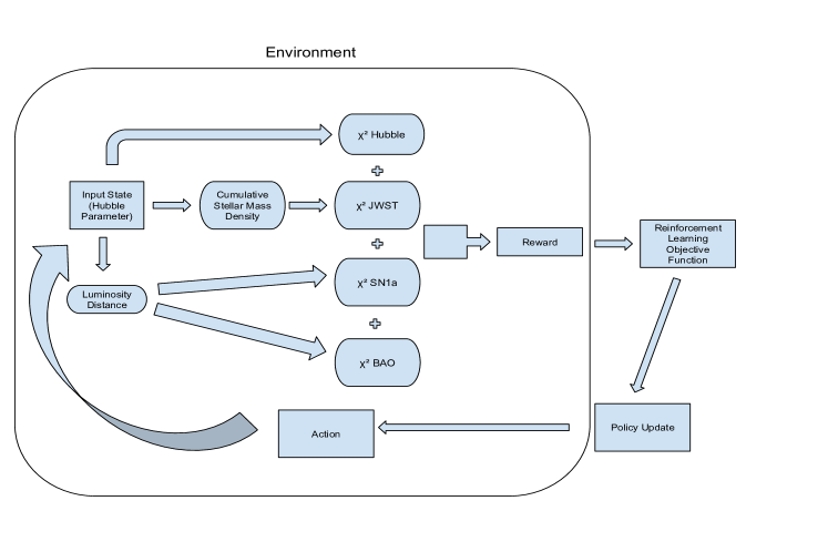
The pipeline architecture to obtain the model-agnostic best-fit scenario is shown in Fig. (1). The architecture has two main parts: (i) the environment, which includes observations, rewards, and actions, and (ii) the RL algorithm, which tries to find the true distribution of actions given an input state.

In the environment, the state represents the possible value of the Hubble parameter at some time step. Initially, the algorithm explores possible states by randomly generating a set of states ranging from the recombination epoch to the present epoch . Based on each Hubble parameter’s evolution, we numerically solve the second-order differential equation of matter density contrast $\delta_{m}(N)$ given by:

$$\frac{d^{2}\delta_{m}}{dN^{2}}+\frac{1}{2}\big{[}1-3w_{\text{eff}}(N)\big{]}\frac{d\delta_{m}}{dN}=\frac{3}{2}\Omega_{m}\delta_{m}\,,\quad\mbox{such that}\quad w_{\text{eff}}(N)=-1-\frac{2}{3}\frac{H^{\prime}(N)}{H(N)}\,,$$ (17)

with the initial conditions $\delta_{m}(N)=\delta_{m}^{\prime}(N)=0.001$ at $N=-7$. Using $\delta_{m}(N)$ and the standard form of the Transfer function $T(k)$, we calculate the cumulative stellar mass density (Eq. 8), which helps us get $\chi^{2}_{\text{JWST}}$. We also obtain luminosity distances to calculate $\chi^{2}_{\text{SN1a}}$ and $\chi^{2}_{\text{BAO}}$.

For each episode of our training, we calculate the sum of all $\chi^{2}$ values to get the reward. This reward information is sent to the RL objective function (Eq. 26). The algorithm uses a “gradient ascent” strategy to maximize the reward, updating its exploration policy based on this. The policy determines which action should be taken at each time step. The policy is updated until the distribution of actions for each time step becomes stable. Once stabilized, the algorithm selects actions with the highest probability in a given state, leading to the saturation of accumulated rewards, which indicates that the model is now trained.

4 Results

Once the model is trained, it is able to select the optimized actions for each state. In particular, given a state-value of $H(z)$ at a particular time, based on the distribution of actions, it can figure out what would be the Hubble parameter value at next time step. The obtained evolution is shown in Fig. (2), in which the solid line (best-fit) represents the predicted state values, and the dashed line represents the $1\sigma$ error region . The best-fit line corresponds to the state values of the optimized model . One can see that near the present epoch ($z=0$), it predicts the Hubble parameter to be significantly larger than the Planck best-fit value of $67.66$ km/s/Mpc. This enhancement in $H_{0}$ can be attributed to the fact that DE could possibly be phantom in nature at late-times. This result is completely opposite to the DESI’s combined estimates with other datasets such as SN1a, where it was found that DE equation of state is quite larger than $-1$ (as also mentioned earlier). Since, the predicted $H(z)$ profile, while not accurately reconstructable using the Chevallier-Polarski-Linder (CPL) parameterization, in our case it is challenging to determine the precise evolution of DE equation of state.

Figure 2: Evolutionary profile of the Hubble parameter $H(z)$ for $z\in[0,1]$ obtained using the RL framework. The solid line represent the median value, whereas dashed lines represent $1\sigma$ error bar region.

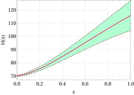
Nevertheless, we have found that the tension between the Planck data and the SH0ES measurement, which is at the $5\sigma$ level, is significantly reduced to the $2.6\sigma$ level in our case. In order to check the goodness of fit of our result with respect to the $\Lambda$CDM model, we compare the minimized $\chi^{2}$ value for both cases. We find that

$$\Delta\chi^{2}:=\chi^{2}_{\text{RL}}-\chi^{2}_{\Lambda CDM}=-6.94\,.$$ (18)

The best-fit parameters for the $\Lambda$CDM model,comes out to be $\Omega_{m}^{(0)}=0.322$, and $H_{0}=68.2$ km/s/Mpc. The negative sign of $\Delta\chi^{2}$ shows the betterment of our fit as compared to the $\Lambda$CDM and the similar models which mimics it at both early and late times.

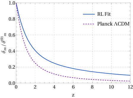
For the obtained $H(z)$ profile, we have numerically determined the evolution of the matter density contrast $\delta_{m}(z)$, normalized to unity at the present epoch, as shown in Fig.,(3). In this figure, it can be observed that at higher redshifts, $D(z)$ or $\delta_{m}(z)/\delta^{(0)}_{m}$ obtained through RL tends to be larger at all epochs compared to what is predicted by the Planck best-fit value for the $\Lambda$CDM model. This occurs because phantom DE introduces more friction to the evolution of $\delta_{m}(z)$ by also decreasing the contribution of the source term. Consequently, $D(z)$ decreases comparatively slowly in the past than in the $\Lambda$CDM model. At around redshift $z=10$, we have found that the ratio between our best-fit $D(z)$ and $D(z)_{\Lambda CDM}$, i.e., $D(z)/D(z)_{\Lambda CDM}$, is $3.46$.

The observed enhancement in the matter density contrast can exponentially affect the cumulative stellar mass density at higher redshifts for all comoving scales. In particular, enhancement in $D(z)$ will enhance the matter power spectrum $P(k)$, which then enhance the halo mass function for a given mass $M$. This enhancement will then exponentially affect the cumulative stellar mass density.

Figure 3: Evolutionary profile of the normalized matter density contrast with $z\in[0,12]$ for $\Lambda$CDM (in dashed) and for the predicted by RL.

(a) Cumulative stellar mass density profiles at $z\simeq 8$ for RL and $\Lambda$CDM.

(b) Cumulative stellar mass density profiles at $z\simeq 9$ for RL and $\Lambda$CDM.

Figure 4: Comparative analysis of cumulative stellar mass density profiles at different redshifts.

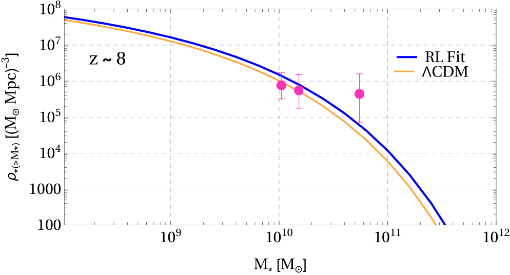
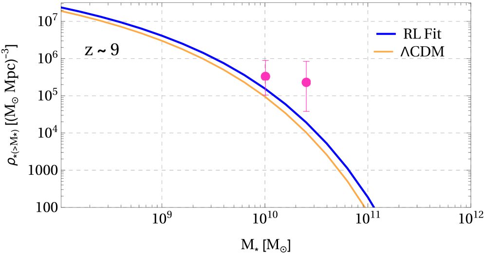
Figs. (4(a)) and (4(b)) depict the cumulative stellar mass density as a function of $M_{\ast}$ (in solar mass $M_{\odot}$) for redshifts $8$ and $9$, respectively. These results show that the RL framework predicts a higher cumulative stellar mass density compared to the $\Lambda$CDM model. Notably, at redshift $z=9$, the $\Lambda$CDM model significantly underestimates the stellar mass density required to match observational data from the JWST, which suggests a need for higher densities to align with observational data. Here we note that only for the JWST dataset, we have found $\Delta\chi^{2}_{\text{JWST}}=-5.5$. The RL model, however, provides a closer match to these observations, indicating that it better captures the large densities necessary at high redshifts.

The trained model not only suggests the reduction of the $H_{0}$ tension but also the tension with the JWST data. Since both early and late-time tensions are reduced, it indicates that the fundamental nature of DE, in overall, likely to be significantly differ with that of the cosmological constant.

5 Conclusion

In this paper, we have studied discrepancies between the early and late time observational data, such as JWST and DESI, and the underline cosmology from a completely different standpoint, i.e. by utilizing the model-independent reinforcement learning. As the data from various phenomena such as large-scale structure or BAO, which are inexplicable within our current understanding of theoretical models, it necessitates the use of a model-independent technique, specifically one that is free from any cosmological pre-assumptions. The main objective to implement this technique is to figure out if there exists any unknown feature in the data in the data that our conventional cosmological models are unable to take them in account due to pre-imposed constraints on their formulation.

In order to estimate the statistical quantity to observe the goodness of fit, we have formulated this reward based technique in terms of $\chi^{2}$ which has directed the RL agent to choose the policy which leads to the higher cumulative reward or lower $\chi^{2}$ function over an episode. By changing the policy at each epoch, the model tries to find the optimized reward, which at the end of the training procedure comes out to be statistically more preferable than the $\Lambda$CDM model by a significant factor.

With our constructing of the pipeline to make the agent learn the observational data that are at different redshifts, we have found that the trained model predicts underline cosmology to be significantly distinguishable at late times due to its preference to the phantom behavior of DE. This is interesting in the sense that the model naturally finds this as the preferable DE candidate over other and it indeed helps in reducing atleast the late-time tension, as shown in [13] using genetic algorithm. We have shown that this phantom nature not only milder the tensions that is existed between Planck $\Lambda$CDM model and SH0ES, but also tends to reduce the tension with the JWST observations. In particular, the consequence of this departure from the base $\Lambda$CDM model, gets reflected in the growth of matter perturbations, which shows a comparatively enhancement in the growth function of matter perturbations at all times upto the present epoch (3). The enhanced growth function then acts as a key ingredient to enhance the cumulative stellar mass density at higher redshifts, which suggests a potential explanation to the given JWST data (see figs. (4(a) and 4(b)). Also, we have observed that our results are in contrast to the recent DESI observations which, within the template of CPL ansatz, suggests a very large equation of state parameter for DE at the current epoch. In contrast to that, we have not found any such discrepancy, as our result prefers lower than $-1$ DE equation of state. This might be due to the fact of our model-independent approach in which there are no such theoretical constraints. Finally, it will be interesting to determine which cosmological model our RL-based fit closely matches, or what cosmological model can be reconstructed based on our results regarding the predicted evolutionary history of the universe. We are currently working on these lines and will try to report soon.

Appendix

5.1 Proximal Policy Optimization

The main working principle of PPO is to optimize the policy of selecting actions at each state by exploring the environment and taking feedback from it. The goal is to maximise the expected reward $J(\theta)$ by updating the policy parameter $\theta$:

$$J(\theta)=\mathrm{E}\left[\sum_{t=0}^{T}\gamma^{t}r_{t}\right]\,.$$ (19)

By using the policy gradient theorem, the rate of change of expected reward with the policy parameter $\theta$ can be written as:

$$\nabla_{\theta}J(\theta)=\mathrm{E}_{s\sim\rho^{\pi},a\sim\pi_{\theta}}\left[\nabla_{\theta}\log\pi_{\theta}(a|s)\hat{A}(s,a)\right]\,,$$ (20)

where $\hat{A}(s,a)$ is the advantage function. It is based on the gradient of the accumulated reward $J(\theta)$ with respect to the policy parameter $\theta$ as:

$$\nabla_{\theta}J(\theta)=\mathrm{E}_{s\sim\rho^{\pi},a\sim\pi_{\theta}}\left[\nabla_{\theta}\log\pi_{\theta}(a|s)\hat{A}(s,a)\right]\,.$$ (21)

PPO uses the concept of clipped objective to ensure that the updates to the policy are not too large. The clipped surrogate objective is defined as:

$$L^{\text{CLIP}}(\theta)=\mathrm{E}_{t}\left[min\{r_{t}(\theta)\hat{A}_{t},clip\{r_{t}(\theta),1-\epsilon,1+\epsilon\}\hat{A}_{t}\}\right]\,,$$ (22)

where $r_{t}(\theta)=\frac{\pi_{\theta}(a_{t}|s_{t})}{\pi_{\theta_{old}}(a_{t}|s_{t})}$ is the probability ratio, and $\epsilon\simeq 0.2$ is an hyperparameter that controls the clipping range.

The policy parameter $\theta$ are updated to maximise the clipped surrogate objective as:

$$\theta\leftarrow\theta+\alpha\nabla_{\theta}L^{\text{CLIP}}(\theta)\,,\quad\mbox{where}\quad\alpha:=\text{Learning rate}\,.$$ (23)

It also uses the value function $V_{\theta}(s_{t})$ to estimate the expected return. The value function loss is defined as:

$$L^{\text{VF}}(\theta)=\mathrm{E}_{t}\left[(V_{\theta}(s_{t})-R_{t})^{2}\right]\,.$$ (24)

To encourage exploration, the Entropy is also added to the objective function:

$$L^{\text{S}}(\theta)=\mathrm{E}_{t}\left[\mathcal{H}(\pi_{\theta}(\cdot|s_{t}))\right]\,.$$ (25)

Finally the total objective function is given as:

$$L(\theta)=\mathrm{E}_{t}\left[L^{\text{CLIP}}(\theta)-c_{1}L^{\text{VF}}(\theta)+c_{2}L^{\text{S}}(\theta)\right]\,,$$ (26)

where $c_{1}$ and $c_{2}$ are some coefficients.

5.2 Savitzky-Golay Smoothing Filter

The Savitzky-Golay filter is a filtering technique that is used to smooth data while preserving the shape and important details in the data. For a given set of data points $y_{i}$, where $i\in[0,N-1]$, the smoothed value $\hat{y}_{i}$ s obtained by fitting a polynomial of order $p$ over a window of length $2m+1$ centered around each point. The formula for the smoothed value is:

$$\hat{y}_{i}=\sum_{j=-m}^{m}c_{j}y_{i+j}\,,$$ (27)

where $c_{j}$ are the filter coefficients, and $y_{i+j}$ are the original data points within the window centered at $y_{i}$. The polynomial $P(x)$ of degree $p$ can be written as:

$$P(x)=a_{0}+a_{1}x+a_{2}x^{2}\cdot+a_{p}x^{p}\,.$$ (28)

For every data point $y_{i}$, it choose a window centered on $y_{i}$ and fit the above polynomial to the points: $\{y_{i-m},y_{i-m+1}\dots y_{i}\dots y_{i+m-1},y_{i+m}\}$.

To construct the Vandermonde matrix $A$, it use the relative positions within the window. If the window has length $2m+1$ and is centered around $y_{i}$, the relative positions are $k=-m,-m+1,\dots,0,\dots,m-1,m$. The Vandermonde matrix $A$ is: $\begin{bmatrix}(-m)^{0}&(-m)^{1}&(-m)^{2}&\cdots&(-m)^{p}\\ (-m+1)^{0}&(-m+1)^{1}&(-m+1)^{2}&\cdots&(-m+1)^{p}\\ \vdots&\vdots&\vdots&\ddots&\vdots\\ 0^{0}&0^{1}&0^{2}&\cdots&0^{p}\\ \vdots&\vdots&\vdots&\ddots&\vdots\\ (m-1)^{0}&(m-1)^{1}&(m-1)^{2}&\cdots&(m-1)^{p}\\ m^{0}&m^{1}&m^{2}&\cdots&m^{p}\,.\\ \end{bmatrix}$

In the abaove matrix, each row corresponds to a data point within the window, and each column corresponds to a power of the relative position from the chosen point. Now, the filter coefficients $c_{j}$ can be obtained using the least squares: $Aa=y$, where $y$ is the vector of data points in the window and $a$ is the vector of polynomial coefficients. The coefficients $c_{j}$ are derived from the first row of the pseudoinverse of the Vandermonde matrix $A$.

The smoothed value $\hat{y}_{i}$ is then given by:

$$\hat{y}_{i}=\sum_{j=-m}^{m}c_{j}y_{i+j}\,.$$ (29)

References

- [1] L. Amendola and S. Tsujikawa, Dark Energy: Theory and Observations, Cambridge University Press, United Kingdom (2010).
- [2] E.J. Copeland, M. Sami and S. Tsujikawa, Dynamics of dark energy, Int. J. Mod. Phys. D 15 (2006) 1753, arXiv: hep-th/0603057.
- [3] J.A. Frieman, M.S. Turner and D. Huterer, Dark energy and the accelerating universe, Ann. Rev. Astron. Astrophys. 46 (2008) 385, arXiv: 0803.0982[astro-ph].
- [4] E. Di Valentino et al., In the realm of the Hubble tension—a review of solutions, Class. Quant. Grav. 38 (2021) 15, 153001, arXiv: 2103.01183 [astro-ph.CO].
- [5] S. Vagnozzi, Seven hints that early-time new physics alone is not sufficient to solve the Hubble tension, Universe 9 (2023) 393, arXiv: 2308.16628 [astro-ph.CO].
- [6] A. G. Riess et. al., A 2.4% Determination of the Local Value of the Hubble Constant, Astrophys. J., 826(1) (2016) 56, arXiv: 1604.01424 [astro-ph.CO].
- [7] K. C. Wong et. al., H0LiCOW – XIII. A 2.4 per cent measurement of H0 from lensed quasars: 5.3 tension between early- and late-Universe probes, Mon. Not. Roy. Astron. Soc., 498(1) (2020) 1420-1439, arXiv: 1907.04869 [astro-ph.CO].
- [8] N. Aghanim et. al., Planck 2018 results. VI. Cosmological parameters, Astron. Astrophys. 641 (2020) A6, arXiv: 1807.06209 [astro-ph.CO].
- [9] M. Boylan-Kolchin, Stress testing CDM with high-redshift galaxy candidates, Nature Astron. 7(6) (2023) 731–735,arXiv: 2208.01611 [astro-ph.CO].
- [10] I. Labbe et. al., A population of red candidate massive galaxies ~600 Myr after the Big Bang, Nature 616(7956) (2023) 266–269, arXiv: 2207.12446 [astro-ph.GA].
- [11] A.G. Adame et. al., DESI 2024 VI: Cosmological Constraints from the Measurements of Baryon Acoustic Oscillations, arXiv: 2404.03002 [astro-ph.CO].
- [12] Y. Tada, T. Terada, Quintessential interpretation of the evolving dark energy in light of DESI observations, Phys. Rev. D 109(12) (2024) L121305, arXiv: 2404.05722 [astro-ph.CO].
- [13] M. R. Gangopadhyay, M. Sami, M. K. Sharma, Phantom dark energy as a natural selection of evolutionary processes a^ la genetic algorithm and cosmological tensions, Phys. Rev. D 108(10) (2023) 103526, arXiv: 2303.07301 [astro-ph.CO].
- [14] D. Bousis, L. Perivolaropoulos, Hubble tension tomography: BAO vs SnIa distance tension, arXiv: 2405.07039 [astro-ph.CO].
- [15] M. Forconi, W. Giarè, O.Mena, Ruchika, E. Di Valentino, A double take on early and interacting dark energy from JWST, JCAP 05 (2024) 097, arXiv: 2312.11074 [astro-ph.CO].
- [16] P. Wang et. al., Exploring the Dark Energy Equation of State with JWST, arXiv: 2307.11374 [astro-ph.CO].
- [17] S. A. Adil et. al., Dark energy in light of the early JWST observations: case for a negative cosmological constant?, JCAP 10 (2023) 072, arXiv: 2307.12763 [astro-ph.CO].
- [18] Yi-Ying Wang et. al., Modeling the JWST High-redshift Galaxies with a General Formation Scenario and the Consistency with the CDM Model, Astrophys. J. Lett. 954(2) (2023) L48, arXiv: 2307.12487 [astro-ph.GA].
- [19] M. G. Dainotti, G. Bargiacchi, M. Bogdan, S. Capozziello, S. Nagataki, Reduced uncertainties up to on the Hubble constant and the matter density with the SNe Ia with a new statistical analysis, arXiv: 2303.06974 [astro-ph.CO].
- [20] J. Sakstein, and M. Trodden, Early Dark Energy from Massive Neutrinos as a Natural Resolution of the Hubble Tension, Phys. Rev. Lett. 124(16) (2020) 161301, arXiv: 1911.11760 [astro-ph.CO].
- [21] G. Alestas, L. Kazantzidis, and L. Perivolaropoulos, tension, phantom dark energy, and cosmological parameter degeneracies, Phys. Rev. D 101(12) (2020) 123516, arXiv: 2004.08363 [astro-ph.CO].
- [22] R. Arjona, and S. Nesseris, What can Machine Learning tell us about the background expansion of the Universe?, Phys. Rev. D 101(12) (2020) 123525, arXiv: 1910.01529 [astro-ph.CO].
- [23] S. A. Adil, M. R. Gangopadhyay, M. Sami, and M. K. Sharma, Late-time acceleration due to a generic modification of gravity and the Hubble tension, Phys. Rev. D 104(10) (2021) 103534, arXiv: 2106.03093 [astro-ph.CO].
- [24] M. R. Gangopadhyay, S. K. J. Pacif, M. Sami, and M. K. Sharma, Generic Modification of Gravity, Late Time Acceleration and Hubble Tension, Universe 9(2) (2023) 83, arXiv: 2211.12041 [gr-qc].
- [25] G. Alestas, and L. Perivolaropoulos, Late-time approaches to the Hubble tension deforming H(z), worsen the growth tension, Mon. Not. Roy. Astron. Soc. 504(3) (2021) 3956-3962, arXiv: 2103.04045 [astro-ph.CO].
- [26] H. Van Hasselt, A. Guez, D. Silver, Deep reinforcement learning with double q-learning, Proceedings of the AAAI conference on artificial intelligence, 30(1) (2016), arXiv: 1509.06461 [cs.LG].
- [27] J. Schulman, et al. Proximal policy optimization algorithms, arXiv:1707.06347.
- [28] R. K. Sheth, H.J. Mo, G. Tormen, Ellipsoidal collapse and an improved model for the number and spatial distribution of dark matter haloes, Mon. Not. Roy. Astron. Soc. 323 (2001) 1, arXiv: astro-ph/9907024.
- [29] M. K. Sharma, M. Sami, D. F. Mota, Generic Predictions for Primordial Perturbations and their implications, arXiv: 2401.11142 [astro-ph.CO].
- [30] S. Cao, J. Ryan, B. Ratra, Using Pantheon and DES supernova, baryon acoustic oscillation, and Hubble parameter data to constrain the Hubble constant, dark energy dynamics, and spatial curvature, Mon. Not. Roy. Astron. Soc. 504(1) (2021) 300-310, arXiv: 2101.08817 [astro-ph.CO].
- [31] S. Nesseris, J. García-Bellido, Comparative analysis of model-independent methods for exploring the nature of dark energy, Phys. Rev. D 88(6) (2013) 063521, arXiv: 1306.4885 [astro-ph.CO].
- [32] H. Padmanabhan, A. Loeb, Alleviating the Need for Exponential Evolution of JWST Galaxies in M⊙ Haloes at z 10 by a Modified CDM Power Spectrum, Astrophys. J. Lett. 953(1) (2023) L4, arXiv: 2306.04684 [astro-ph.CO].