A model independent approach to the study of structure growth in gravity
Abstract
Over the last decade, much attention has been given to the study of modified gravity theories to find a more natural explanation for the late-time acceleration of the Universe. Particular attention has focused on the so-called dark energy models. Instead of focusing on a particular f(R) model, we present a completely model-independent approach to study the background dynamics and the growth of matter density perturbations for those f(R) models that mimic the CDM evolution at the background level. We do this by characterising the dynamics of the gravitational field using a set of dimensionless variables and using cosmography to determine the expansion history. We then illustrate the integrity of this method by fixing the cosmography to be the same as an exact CDM model, allowing us to test the solution. We compare the exact evolution of the density contrast and growth index with what one obtains from various levels of the quasi-static approximation, without choosing the form of dark energy.
keywords:
Modified Gravity, Structure Growth, Cosmography1 Introduction
For almost two decades, the cosmological constant has remained the simplest and most compelling explanation for what is driving the present-day accelerated expansion of the universe, assuming of course that the geometry of the universe is well described by the Robertson-Walker metric. While the CDM model Blumenthal et al. (1984); Ostriker & Steinhardt (1995) is by far the simplest theoretical description, it is not without its flaws. Dicke was the first to bring up the issue of ‘fine-tuning’ in the cosmological context Dicke (1961) - that a slightly larger value of would render large-scale structure impossible. Additionally, the dark energy density having an equal order of magnitude to the matter density at present, despite contrary evolution histories, has been aptly termed the ‘coincidence problem’ Steinhardt (1998). There is also an alarming disagreement between the observed value of the vacuum energy density and the much larger zero-point energy determined from quantum field theory Adler et al. (1995). Finally, the most recent DESI results appear to support a theory of evolving dark energy parameterised by the CDM model Tada & Terada (2024).
In light of these issues, various modifications of General Relativity (GR) have been investigated. One of the simplest non-trivial extensions of GR has an action that is non-linear in the Ricci curvature and/or other curvature invariants Stelle (1978); De Felice & Tsujikawa (2010); Sotiriou & Faraoni (2010). An important property of these theories is that the field equations can be constructed in a way which makes comparisons with GR straightforward. This is done by moving all the non-linear corrections onto the right-hand side of the field equations. In this way, we can define an “effective” source term, known as the curvature fluid. One of the properties of the curvature fluid is that it naturally violates the strong energy condition, allowing for a curvature-fluid-driven period of late-time cosmological acceleration Carroll et al. (2004); Capozziello & Francaviglia (2008). Unfortunately, this comes at the cost of having to study a much more complicated (fourth-order) set of field equations. This leads to considerable challenges in determining exact and numerical solutions which can be confronted with observations. These difficulties can be addressed somewhat by using dynamical systems methods Carloni et al. (2005); Carloni & Dunsby (2007); Carloni et al. (2009); Abdelwahab et al. (2012). Guided by the Friedmann constraint, a set of dimensionless dynamical variables can be defined, providing a relatively simple method for obtaining exact solutions (via the equilibrium points of the system) and a description of the global dynamics of these models. Unfortunately, the dynamical system obtained is only autonomous for particularly simple forms of and each theory has to be analysed separately. This is due to a term remaining in the equations involving and its first and second derivatives with respect to , which cannot be expressed in terms of the dynamical system variables in general Carloni et al. (2009). This issue can be resolved by introducing additional variables and parameters, but the functional form still needs to be specified prior to analysing the cosmological dynamics Carloni (2015).
Recently it was noticed that this problem can be solved more elegantly by writing in terms of the cosmographic parameters Chakraborty et al. (2021). In this way, it is possible to write a complete set of differential equations for any theory. Of course, things are not quite that simple. Since the cosmographic series satisfies an infinite hierarchy of equations, a closed system is only obtained when one fixes the expansion history, which determines an algebraic relationship between the cosmographic parameters. Nevertheless, this approach proves to be more general and more closely linked to observations than any other approach thus far.
In this work, we build on Chakraborty et al. (2021), focusing on developing a framework for modelling the growth function in a way which is independent of the choice of . All other work in this area either fixes from the onset or uses some parameterisation to describe the modification to GR (see for example Carloni & Dunsby (2007); Ananda et al. (2009); Tsujikawa et al. (2009); Pogosian & Silvestri (2008); Bean et al. (2007); Gannouji et al. (2009); Gannouji & Polarski (2008); Narikawa & Yamamoto (2009); Abebe et al. (2013)). We find that our approach is able to capture features that have been observed in various model-specific methods in a completely general way. Also, by comparing the exact equations with various levels of approximation (semi and full quasi-static (QS)), we are able to determine the shortcomings of the full QS method on large scales, where the perturbations have not spent significant time in the regime and thus tend to be closer to CDM.
The outline of the paper is as follows. In Section 2, we give the cosmological equations for gravity and describe the general model-dependent dynamical systems approach. In Section 3, we give some background on cosmography and describe the cosmographic-based, model-independent dynamical systems formulation in Section 4. In Section 5 we derive the 1+3 covariant equations describing the growth of structure in a way which is independent of the cosmography and the choice of . In Sections 6 and 7, we explain why choosing the cosmographic condition, leads to a background that mimics CDM in gravity and in Section 8 we apply this condition to the model-independent background and perturbation equations.
Natural units () are used throughout this paper, unless otherwise specified. Latin indices run from 0 to 3. Derivatives with respect to time are indicated by and those with respect to the Ricci scalar are indicated as unless otherwise stated. We use the signature and the symbol represents the usual covariant derivative. The Riemann tensor is defined as
| (1) |
where are the Christoffel symbols defined by
| (2) |
The Ricci tensor is defined as the contraction of the first and third indices of the Riemann tensor
| (3) |
The action for gravity in natural units is written as
| (4) |
where is the Ricci scalar, is a general function (of at least ) of the Ricci scalar and is the matter Lagrangian.
2 Cosmological Equations for gravity
2.1 Background FLRW equations
In a spatially flat FLRW background, the equations governing the expansion of the Universe are given by the modified Friedmann and Raychaudhuri equations:
| (5) | ||||
| (6) |
where represents the energy density of standard matter, a prime represents the derivative with respect to , is the Hubble parameter defined through the scale factor as
| (7) |
and is the Ricci scalar:
| (8) |
The energy conservation equation for standard matter is given by
| (9) |
where is the equation of state parameter for standard matter. Two requirements for must be satisfied to maintain the stability of the model. These are:
-
•
to prevent a potential ghost degree of freedom, and
-
•
, at least during the early epoch of matter domination, to prevent an instability in the growth of curvature perturbations (Dolgov-Kawasaki instability).
2.2 Dynamical system analysis
A general dynamical system for gravity in flat space can be expressed in terms of the expansion-normalised dynamical dimensionless variables,
| (10) |
Substituting these into the Friedmann equation (5) gives the following constraint,
| (11) |
allowing the dimension of the system to be reduced to 3.
The variables (10) are differentiated with respect to the number of e-foldings, , and equations 8 and 9 are used to produce the full dynamical system:
| (12a) | ||||
| (12b) | ||||
| (12c) | ||||
| (12d) | ||||
where is defined as
| (13) |
To close the system, it is necessary to express in terms of the dynamical variables , , and . Finding and subsequently requires the invertibility of the relation . This has previously been a limitation on which models of can be studied with this method. Alternative methods have been proposed to tackle this issue, generally involving the introduction of further parameters or variables. In Carloni (2015) the dynamical system was reformulated to include the variables,
| (14) |
where is a constant having the dimension of mass specific to the theory under consideration. The variables and can be related to the cosmographic deceleration () and jerk () parameters, respectively. Expressing these as a dynamical system using the same method as above yields a 4-dimensional phase space. This alternative introduces two auxiliary quantities, and (see In Carloni (2015) for their definition), instead of the single auxiliary quantity , used in the earlier formulation. A closed autonomous dynamical system can be achieved by expressing these auxiliary quantities in terms of the dynamical variables. Unlike the previous method, which depends on the invertibility of a specific relation to find , this alternative approach avoids this limitation by defining and as functions of and . Depending on the form of , the expressions for and can end up becoming very complex. The benefit is that this method can handle any form of .
The drawback of these approaches (including those in the previous sections) is that they adopt a top-down approach, requiring the functional form of to be specified beforehand. The cosmological dynamics of a given can then be analyzed using one of these methods. This means that investigating consequences of dark energy theories must be done model-by-model, which is both inefficient and time-consuming. Ideally one would like to reconstruct the theory of gravity directly from observations or at the very least constrain it by requiring the background cosmology to be consistent to observational data.
It is for this reason that a bottom-up approach, where the form of is totally unspecified to begin with and must satisfy certain cosmological conditions, is developed in the rest of the paper.
3 Some remarks about cosmography
As pointed out in Chakraborty et al. (2021) the key to closing the dynamical system presented in the last section is to write the function in terms of cosmography. The cosmography is determined by a set kinematic (cosmographic) parameters arising from the Taylor expansion of the Hubble parameter Dunsby & Luongo (2016). The -th to -th order cosmographic parameters are as follows:
| (15a) | ||||
| (15b) | ||||
| (15c) | ||||
| (15d) | ||||
| (15e) | ||||
and are called the Hubble, deceleration, jerk, snap, and lerk parameters, respectively. Of course, one could go on to construct even higher-order cosmographic parameters. In fact there are an infinite hierarchy of them 111For some comprehensive reviews see Dunsby & Luongo (2016); Bolotin et al. (2018)..
| (16a) | ||||
| (16b) | ||||
| (16c) | ||||
A given cosmic evolution, if believed to be the solution of either GR or some theory, can always be specified by an algebraic relation between a finite number of cosmographic parameters. Let us elaborate on this point using a simple example from GR. The cosmic evolution corresponding to the standard CDM model of cosmology is a solution of GR plus a cosmological constant, and satisfies the field equation
| (17) |
The above equation contains and the quantities . The first and second time derivatives of (17) give
| (18a) | ||||
| (18b) | ||||
The above equations, along with (17), can be used to solve in terms of from these three equations. If we now, the third time derivative of (17) and substitute the expressions for , the resulting equation can be expressed entirely in terms of the cosmographic parameters Dunajski & Gibbons (2008):
| (19) |
For the special case of spatially flat or vacuum cosmologies, one need not go up to the third derivative of (17) and the snap parameter is therefore unnecessary. This is the case for spatially flat CDM cosmology which gives rise to the simpler and well-known cosmographic condition .
A similar exercise could be performed for cosmic solutions of theories. If a cosmic evolution is believed to be a solution of some theory in the presence of a perfect fluid with a constant equation of state , then it must satisfy the modified Friedmann equation (5), which contains up to the second derivative of the Hubble parameter, , and the quantities . Taking a time derivative of this equation gives the modified Raychaudhuri equation (6), which contains up to the third derivative of the Hubble parameter , and the quantities . These two equations can be used to solve for the two constants in terms of the . If we take the third derivative of the modified Friedmann equation (5) and substitute the expressions for . The resulting equation can be expressed purely in terms of the cosmographic parameters . One does not need to go beyond the lerk parameter, in agreement with the cosmography analysis presented in Capozziello et al. (2008). Again, for spatially flat or vacuum cosmological solutions of theories, one need not go up to the third derivative of (5) and the lerk parameter is unnecessary. For spatially flat and vacuum cosmological solutions, one need not even consider the modified Raychudhuri equation (6) and the modified Friedmann equation itself represents a cosmographic relation going only up to the jerk parameter Dunajski & Gibbons (2008).
4 A model-independent dynamical system formulation
Recently Chakraborty et al. (2021) a model-independent dynamical system formulation was proposed, which does not require one to specify a-priori an model, while still allowing one to obtain a closed autonomous system.
In the standard model-dependent approach, the dynamical system (12) is not closed due to the presence of the model-dependent factor (13). As described in Chakraborty et al. (2021), the key to solving this issue was to write in terms of the cosmographic parameters (15):
| (20) |
using the the Ricci scalar definition (8).
Differentiating (10) and (15) with respect to the redshift , the resulting model-independent dynamical system for a barotropic perfect fluid with equation of state parameter is
| (21a) | ||||
| (21b) | ||||
| (21c) | ||||
| (21d) | ||||
| (21e) | ||||
| (21f) | ||||
where . The constraint (11) and an additional relation coming from the definition of the Ricci scalar:
| (22) |
has been used to eliminate and .
There is a decoupling structure in the above system. The last four equations, which are purely kinematic in nature, by themselves form a closed dynamical system, provided, of course, one specifies a cosmic evolution as 222One can compare this decoupled kinematic dynamical system with the hierarchy of inflationary slow-roll parameters Kinney (2002); Liddle (2003); Spalinski (2007). The gravitational dynamics enters the system through the and equations.
In principle, one could go on and obtain an infinite number of equations since there is an infinite hierarchy of cosmographic parameters, but, as we discussed in Section 3, any cosmic evolution that is a solution of some theory can be expressed as an algebraic constraint involving up to the lerk parameter. Therefore, one does not need to go beyond (LABEL:eq:ds_s). When one tries to reconstruct the functional form starting from a given cosmological solution , one of course believes that there is an underlying theory of which is a solution. The dynamical system formulation based on the cosmographic parameters is in some sense an alternative to the reconstruction method Nojiri et al. (2009); Dunsby et al. (2010); Carloni et al. (2012). Consequently, it is completely justified to take into consideration only up to (LABEL:eq:ds_s). This particular formulation allows one to study the phase space of all those theories that can reproduce a cosmic evolution given by the cosmographic condition , without explicitly reconstructing the underlying form of .
Additionally, it is noted that using the definition of one can write
| (23) |
We recall that the absence of ghost and tachyonic instability requires . Assuming that the condition is met, demanding puts the following constraints on the phase space333This constraint was stated incorrectly in a previous paper Chakraborty et al. (2021) as . Both the constraint and associated plot (see Figure 3) have been amended here.
| (24) |
It follows that only a portion of the phase space is physically viable. The physically viable region of the phase space, where the theory is free from ghost and tachyonic instability, must necessarily satisfy the constraint (24). One should be careful, though; this is not a sufficient condition. It is certainly possible that a region of the phase space satisfying the condition (24) is plagued by both ghost and tachyonic instability ( and ). To be sure, one must explicitly calculate along a phase trajectory of interest. In a region of the phase space, if the condition (24) is satisfied and also the dynamical variable , then one can definitely say that the region is physically viable.
5 Structure growth
5.1 Covariant gauge-invariant density perturbations in gravity
In order to analyse the growth of large scale structure we use the 1+3 Covariant and Gauge Invariant approach introduced by Ellis & Bruni Ellis & Bruni (1989) and developed for theories of gravity in Carloni et al. (2008). Our focus will be on density perturbations, so it will be enough to extract only the scalar parts of the density gradient using a local decomposition Dunsby et al. (1992); Bruni et al. (1992) through repeated application of the operator , where is the projection tensor into the tangent 3-spaces orthogonal to the 4-velocity . We thus define the scalar quantities
| (25) |
representing the fluctuations in the matter energy density , the expansion , the 3-Ricci scalar , the Ricci scalar and its momentum respectively. Here .
We then perform a harmonic decomposition using the eigenfunctions of the spatial Laplace-Beltrami operator defined in Ellis & Bruni (1989); Dunsby et al. (1992); Bruni et al. (1992), , where is the wavenumber and , allowing us to expand every first order quantity in the perturbation equations in terms of the harmonics as
| (26) |
stands for a summation over a discrete index or an integration over a continuous one.
Starting from the equations governing the gravitational dynamics linearised around an FLRW background (see Carloni et al. (2008) for details), one can derive a pair of coupled second order equations describing the evolution of the th mode of density perturbations in gravity.
These equations can be expressed in terms of derivatives of the function and time derivatives of the background Ricci scalar Carloni et al. (2008):
| (27a) | ||||
| (27b) |
Since the system (5.1) is very complicated, we employ the quasi-static (QS) approximation, as is typically done in the literature Silvestri et al. (2013); Noller et al. (2014). This approximation consists of two separate premises, the first being that temporal fluctuations of are suppressed in comparison to the perturbation itself and can thus be neglected, for . This assumption alone allows us to simplify the system to one equation for :
The second QS premise involves the sub-horizon assumption , which leads to the approximation for . This simplifies the system to the recognisable form
| (29) |
which mirrors the quasi-static approximation for the density contrast in the Bardeen perturbation formalism Tsujikawa (2007) when :
| (30) |
The validity of this approximation in the synchronous and conformal gauges has been extensively studied Hojjati et al. (2012); Noller et al. (2014); Sawicki & Bellini (2015) and performs well in certain model-specific, sub-horizon contexts, particularly for models with background evolution very close to CDM De la Cruz-Dombriz et al. (2008). However, concern remains whether neglecting both higher order derivatives and time derivatives of the curvature perturbation is too aggressive Bean et al. (2007) for models deviating from CDM. For this reason, it is better to consider the QS method both including and excluding the higher order derivatives. These are referred to as the semi and full quasi-static approximations respectively from here on.
All of these approaches retains explicit dependence on and are thus only applicable once a particular model of is chosen. Additionally, to study the perturbations in relation to results obtained from dynamical systems analyses, it is necessary to express all quantities in the coefficients in terms of the chosen dynamical systems variables, including up to fourth order derivatives of in the case of the full covariant system. This adds a further restriction on the particular models of which can be studied with this approach.
5.2 Model-independent formulation
As in the background system, this model-dependence can be avoided by employing the cosmographic approach. Time derivatives of the Ricci scalar (8) can be expressed in terms of the cosmographic parameters (15):
| (31a) | ||||
| (31b) | ||||
| (31c) | ||||
| (31d) | ||||
Then, taking time derivatives of increasing order of the Friedmann equation (5) yields higher order derivatives of which can then be expressed exclusively in terms of the dynamical systems variables and derivatives and thus the cosmographic parameters using (31). For example, taking the first time derivative of (5) allows us to express as:
| (32) |
Continuing in this way, we can express all coefficients in (5.1) in terms of the dynamical system variables and the cosmographic parameters, resulting in a pair of second order equations describing the evolution of the th mode of density perturbations in gravity in a totally model-independent way. In terms of the redshift , these are
| (33a) | ||||
| (33b) | ||||
where the dimensionless quantities , and have been used.
This same approach can be applied to the semi and full quasi-static perturbation equations (LABEL:eq:semiQSgeneralnon) and (29), allowing us to express these in a model-independent way. In terms of redshift, the corresponding perturbation equations are respectively
| (34) |
where
and
| (35) |
In the GR limit , we see that system (5.1) (and thus each model-independent method (33) - (35) derived therefrom) reduces to
| (36a) | |||
| (36b) | |||
which gives the well-known equation
| (37) |
for the dust equation of state . Obvious differences between the perturbation equations and those in GR include their fourth-order nature and, most importantly, the scale-dependence of density perturbations for any equation of state. If detected, this would point toward clear deviation from CDM.
5.3 Growth function and growth index for matter perturbations
Additional methods of quantifying the growth of the matter perturbations may provide another way to discriminate between modified gravity models and GR DE models (CDM and otherwise). These include the growth function and growth index , defined by
| (38) |
where is the standard matter density parameter,
| (39) |
where we have used . In the covariant formalism, in terms of redshift, this is equivalently
| (40) |
from which the growth index can be calculated as
| (41) |
When it was introduced, the growth index was taken to be constant at low redshift Peebles (1980); Lightman & Schechter (1990). While there is clear time dependence, this approximation proves appropriate for models within GR with constant or smoothly varying equations of state which display Polarski & Gannouji (2008), with CDM specifically having with very little variation for Fonseca et al. (2019). Deviation from these values, significant time variation on small redshifts and scale-dependence of and could all provide strong evidence of a modification to GR.
6 The cosmographic condition
Before moving on to the main analysis of this paper, we wish to comment on the accuracy and specificity of the CDM cosmographic condition.
It is well known that the CDM model gives rise to a cosmic evolution that corresponds to the cosmographic condition Dunajski & Gibbons (2008). While model independent estimates of the jerk parameter relying on cosmic chronometers and supernovae data are consistent with the CDM condition within Mehrabi & Rezaei (2021); Mukherjee & Banerjee (2021), the reconstructed cosmographic quantities are in good agreement with those of CDM when some specific parametric deviations from the concordance values are assumed in the analysis and then constrained by the data fitting Zhai et al. (2013); Amirhashchi & Amirhashchi (2020); Mukherjee & Banerjee (2016, 2017). However, we think it is necessary at this point to clarify the notion of cosmographic (one may also say kinematic) degeneracy with CDM.
The redshift evolution of the jerk parameter is (see e.g. (Mehrabi & Rezaei, 2021, Eq.(4))):
| (42) |
Solving we obtain Zhai et al. (2013); Amirhashchi & Amirhashchi (2020); Mukherjee & Banerjee (2016, 2017)
| (43) |
where and are two arbitrary constants satisfying . In general, for nonzero and , the family of solutions given by (43) specifies a CDM-like cosmic evolution history, in the sense that it has two clearly defined asymptotic limits: an effective CDM limit at asymptotic past (or ) where the cosmic evolution goes like , and an effective -limit at asymptotic future (or ) where the evolution goes like . The particular solution of the above family, specified by and , corresponds to the particular CDM cosmic history that our universe is going through.
It should be appreciated, though, that the condition by itself, although implying a CDM-like cosmic evolution history, may not necessarily single out the CDM model. This is best understood in terms of the statefinder parameters introduced in Sahni et al. (2003). The first statefinder parameter is precisely the cosmographic jerk parameter , but this alone does not specify a model. Specifying a model requires specification of both the statefinder parameters . If one puts in (Sahni et al., 2003, Eq.3), one sees that the equation may be satisfied in general by other models as well, including dynamical dark energy models and models with a dark sector interaction 444For a phase space analysis of some simple dark sector interaction models satisfying the cosmographic condition , see Chakraborty et al. (2023). For the cases considered in that paper, it was found that achieving the condition , although possible in principle, is still problematic (e.g. the set of acceptable solutions are of measure zero), leading the authors to conclude that within GR and respecting the FLRW symmetry, CDM is still the natural choice for .. However, whatever the inherent model is, it must give rise to an evolution of the form of (43), having clearly defined CDM-limit and -limit with non-zero integration constants , and therefore corresponding to a CDM-like evolution.
Also, note that the condition by itself does not provide either any physical interpretation for the two integration constants and , nor any route of fixing them. A physical meaning of these two arbitrary constants can only be provided with respect to a particular model in mind. For example, in the CDM model, dark matter and dark energy evolve independently, and their energy densities redshift as and respectively. Then and only then could we identify with and with . We could not have concluded the same, for example, had the equation of state of dark energy been dynamical or had there been an interaction in the dark sector. In other words, the functional relationships and are sensitive to the choice of the model Mehrabi & Rezaei (2021) 555For example, if one takes the dark energy to be modeled by a fluid with and still impose kinematic degeneracy with CDM by imposing the condition , one obtains . See (Chakraborty et al., 2023, Eq.17).
In summary, the condition is sufficient for reproducing the kinematics of CDM (i.e. similar cosmic evolution), but not its dynamics (i.e. the model itself). From the astrophysical perspective, this remark means that when testing the cosmic history (43) with respect to cosmographic data, one may very well get and , which however should not be taken naively to represent the abundances of dark matter and dark energy at the present day Zhai et al. (2013).
7 The condition in the context of gravity
In the previous section we have discussed the cosmographic kinematic condition from a generic context. Let us focus now on the model under consideration in this paper, i.e., a late time model with no dark-sector interaction and see what the condition implies in this case. The cosmological field equations (5),(6) can be rearranged in the following form
| (44a) | |||
| (44b) | |||
where is the energy density of the non-relativistic matter, and we have defined the energy density and pressure of the dark matter as follows
| (45a) | ||||
| (45b) | ||||
The dark energy equation of state is
| (46) |
Using the field equations (44a) the above can be written as
| (47) |
In this form, the non-relativistic matter and the dark energy is separately conserved
| (48a) | |||
| (48b) | |||
Dividing the numerator and denominator by and utilizing the definitions of the dynamical variables and the cosmographic parameters, we arrive at
| (49) |
where in the last step we have utilized the relation (22) and is the usual matter density parameter defined in (39) which obeys the dynamical equation
| (50) |
Imposing one obtains
| (51) |
Taking a -derivative, utilizing (50) and the first equation of (16) and after performing some rather straightforward steps, one can arrive at the condition . This clearly shows that if the curvature part of the total energy density (i.e. ) behaves like a cosmological constant (), it clearly gives rise to a cosmology with , as expected.
Consider, now, a dynamical dark energy model with . Imposing this in (49) and taking a -derivative, after some straightforward steps one arrives at
| (52) |
One possibility to get , i.e. kinematic degeneracy with CDM is , but it cannot be true for the entire evolution history. Another possibility is , which takes us back to the case . The third possibility is that satisfies the equation
| (53) |
which, upon solving, gives
| (54) |
with . This implies a dark energy equation of state that can be expressed as
| (55) |
Except for the special case , the above corresponds, in general, to a dynamical dark energy, which is still compatible with the cosmographic condition .
One can, in fact, go one step further and calculate from the dark energy conservation equation of (48) that
| (56) |
so that from (44a) one can write
| (57) |
In other words, even though (55) may represent in general a dynamical dark energy, the cosmic evolution is still CDM-like, in the sense that there is a clearly defined effective CDM limit at asymptotic past and a clearly defined effective -limit at asymptotic future. Since we will base our subsequent analysis on the condition , such models are also included in our picture.
8 Application to CDM Cosmology
In this section, we study the background cosmic evolution and growth of matter perturbations for an theory mimicking a CDM cosmic history. As discussed in Section 7, this can be achieved in the cosmographic formulation by fixing . This automatically fixes the snap parameter which in turn fixes the lerk parameter :
| (58) | ||||
| (59) |
Using these expressions, both the background and perturbation equations can be written in terms of the dynamical variables and the deceleration parameter .
8.1 Background evolution for
Fixing closes the dynamical system (21) which, for a dust equation of state (), gives
| (60a) | ||||
| (60b) | ||||
| (60c) | ||||
| (60d) | ||||
We set the initial conditions for the background variables deep in the matter-dominated era666The dynamical system is extremely sensitive to initial conditions, often up to the fourth decimal place. Therefore, setting initial conditions at , if not set very precisely, can result in an incorrect evolution that does not feature a matter-dominated era but rather a scalaron-dominated one for . Setting initial conditions arbitrarily deep in the matter-dominated era then ensures an evolution that complies with CDM.. Initial conditions for and are chosen to match with CDM values, assuming and . For the case, the viability condition (24) gives an upper bound on such that
| (61) |
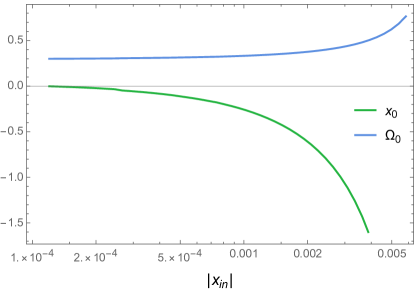
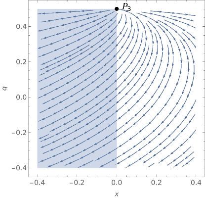
Since , this implies at all redshifts. As encodes the deviation from GR ( being the GR limit), should be small in the matter-dominated era. Selecting exactly how small the initial value of should be is a matter of delicate balance. As shown in Fig 1, for very small values of , the variable evolves to a value , violating the viability condition (24). Additionally, larger values of lead to larger values of , as the deviation from GR grows faster. This in turn affects the value of , driving it further from the observed value of the matter abundance parameter . To achieve this balance, we choose a value of which ensures throughout its evolution up to and results in a value of .
The selected initial conditions are then
| (62) |
which give the background evolution for the variables and shown in Fig 2.
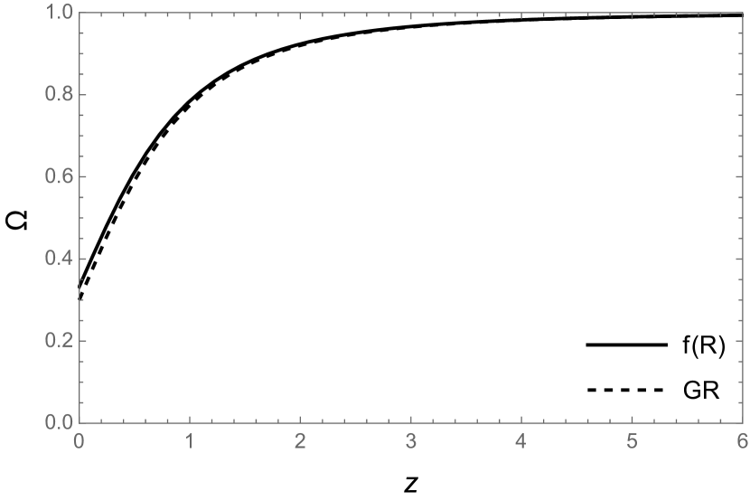
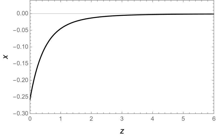
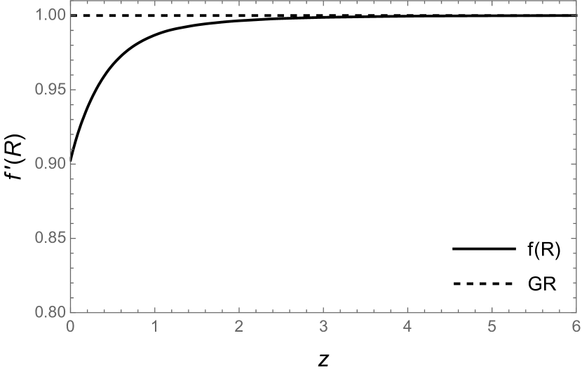
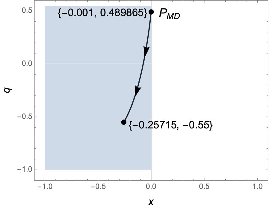
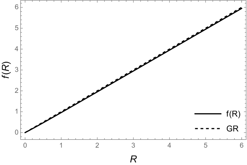
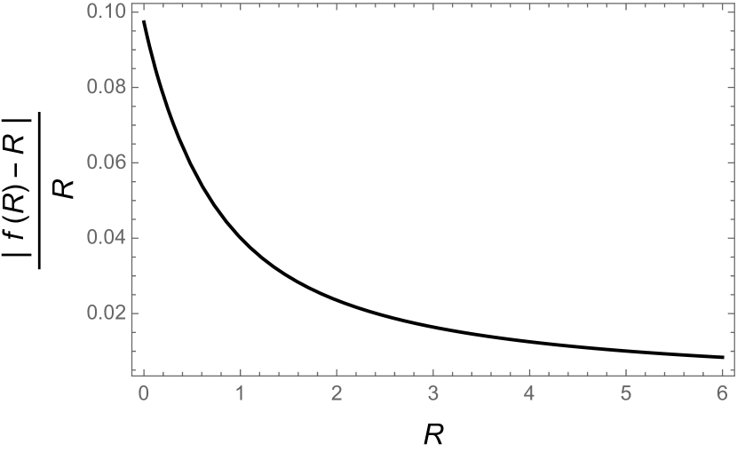
This trajectory meets all the viability conditions since for all time and as shown in Fig 2(c). Since condition (24) is satisfied, this ensures that . For completeness, the numerical expression in Fig 2(c) is used to numerically reconstruct the function , shown in Fig 5(a), and the percentage difference plotted in Fig 5(b) indicates the modification to standard GR.
8.2 Matter perturbations with
We now turn our attention to the matter perturbations for an model with a CDM background and a dust equation of state.
An important consideration in modified gravity theories is the transition from the “GR regime" to the modified regime. In the case of models, this is characterised by the parameter
| (63) |
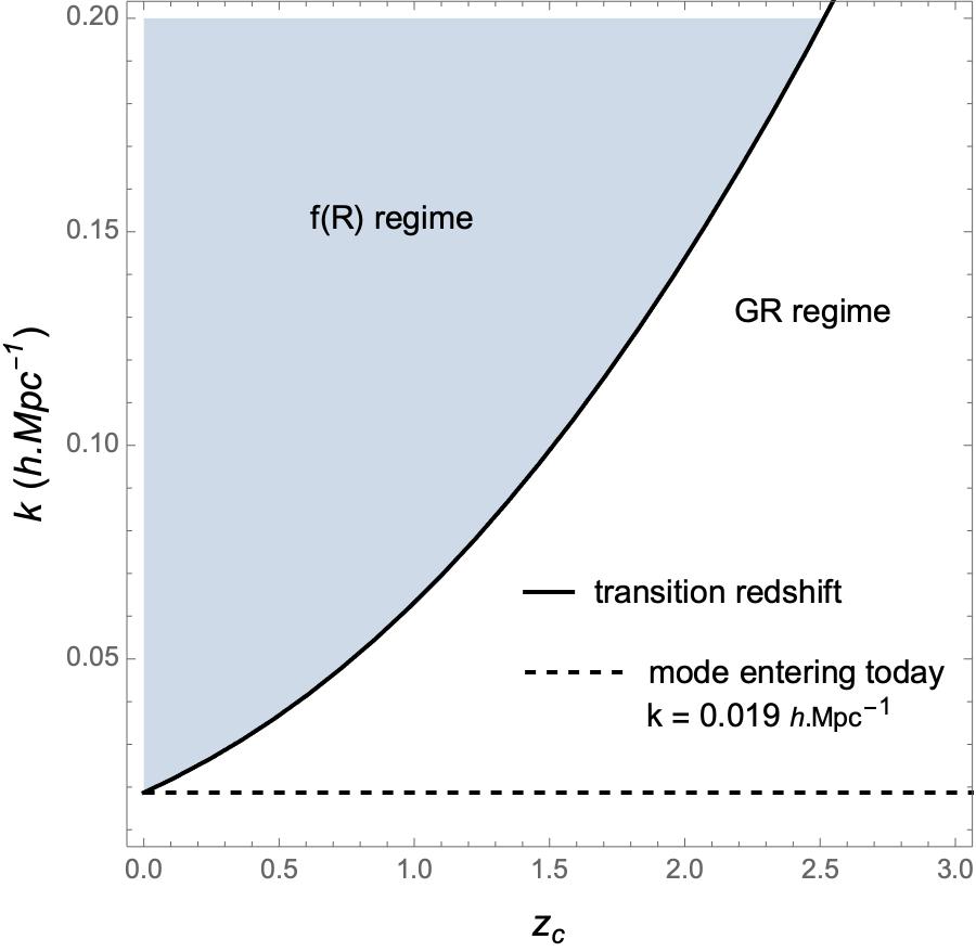
which corresponds to the mass squared of the scalaron in the regime Tsujikawa et al. (2009). In the regime, , the scalaron mass is light, leading to a finite range “fifth force" which is felt by perturbations Pogosian & Silvestri (2008). In the GR regime , the scalaron is massive and the fifth force is suppressed, leading to negligible difference with GR. The transition between regimes is time and scale dependent, meaning different scales (i.e. different -modes) pass from the GR regime into the regime at different times, thus feeling the effect of the deviation from GR differentially. For a perturbation -mode, this transition occurs when , which corresponds to the redshift for which
| (64) |
The scale-dependence of the transition redshift is shown in Fig 6. For smaller scales (larger ), the transition occurs earlier, while larger modes (smaller ) have either entered the regime very close to or have not yet entered at all. In the latter case, these modes are not distinguishable from CDM as they have till now always been in the GR regime.
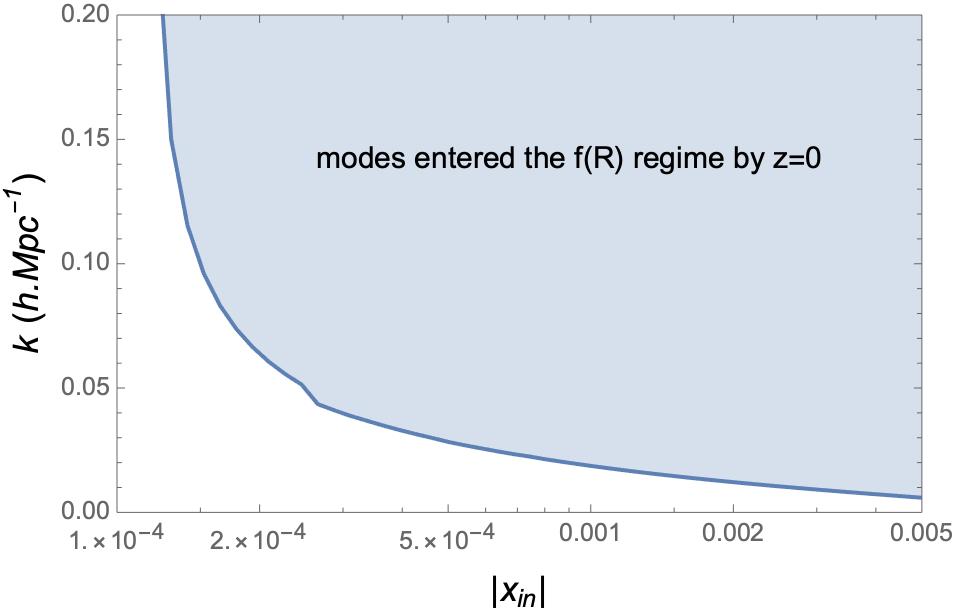
As this transition redshift depends explicitly on the evolution of , varying the initial condition will affect which modes have entered the regime by today. This is shown in Fig 7. For larger values of , say , all the modes relevant to the galaxy power spectrum, , have already entered the regime by today, whereas for very small values of , all of these modes are still inside the GR regime, making them indistinguishable from CDM. This further motivates the choice of , as most of the relevant perturbation modes have entered the regime and the modification is applicable.
As for the background, we set in the perturbation evolution equations for each of the three approaches: the exact covariant, semi QS and full QS approaches. Respectively, these then simplify to
| (65a) | ||||
| , | (65b) | |||
for the exact covariant equations,
| (66) |
with
| (67) |
for the semi QS equation, and
| (68) |
for the full QS method.
In line with Abebe et al. (2013), we set the scale-independent initial conditions in the CMB era at to be
| (69) |
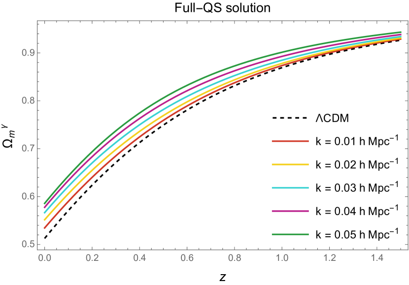
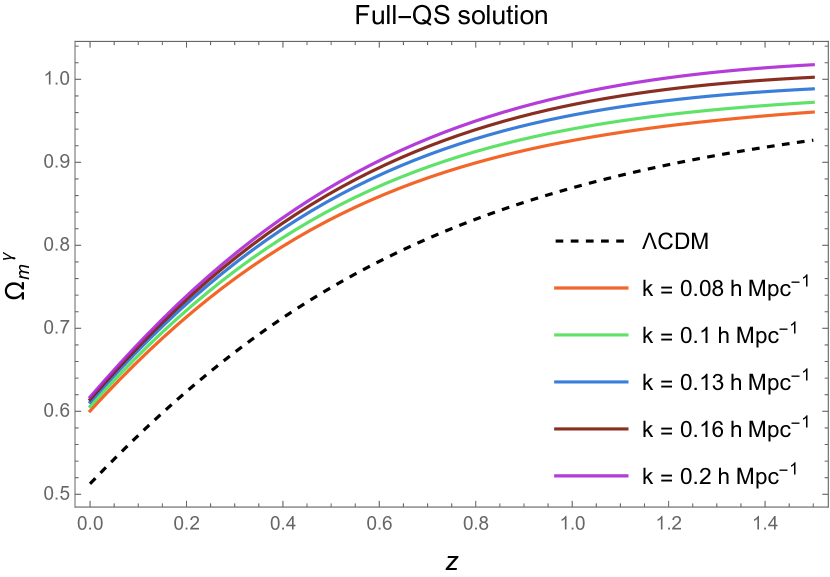
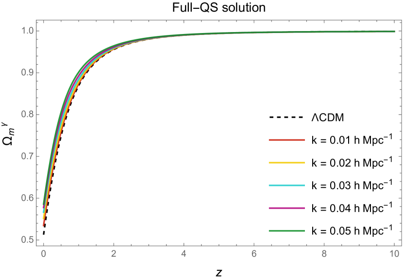
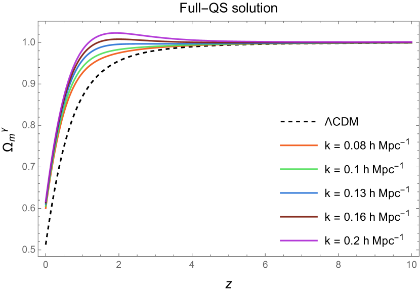
For the background trajectory specified in Figs.4, the associated matter perturbation evolution for each method are shown in Figs. 8 and 9. In Fig. 8 is normalized at to facilitate a comparison with similar plots appearing in model-dependent analysis of Gannouji et al. (2009), which investigates perturbation evolution in Starobinsky’s model. However, such a plot does not clearly portray the scale dependence of at low redshift. To show more clearly the scale-dependence of at very low redshifts (), we have included the corresponding plots where is normalised at in Fig. 9777We believe that normalizing at high redshift is more logical in the sense that at high redshift a viable theory should asymptotically tend to GR, for which there is no scale-dependence..
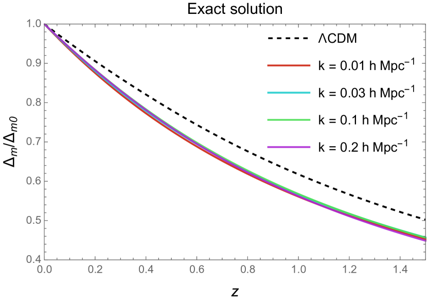
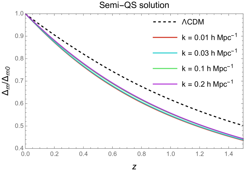
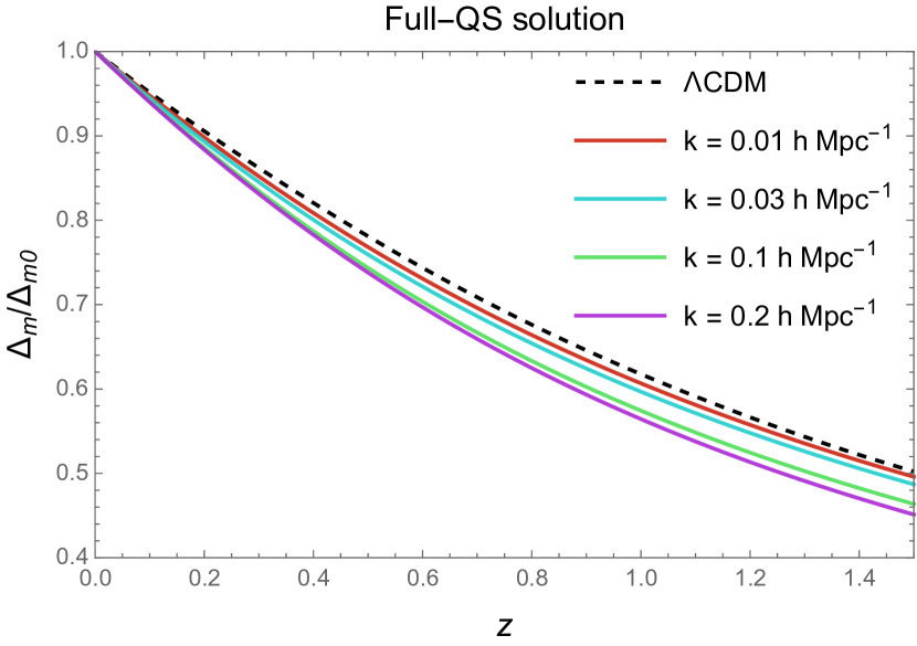
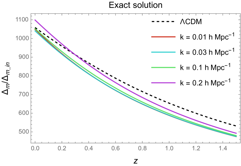
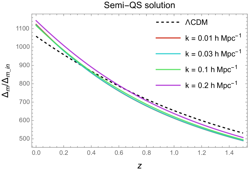
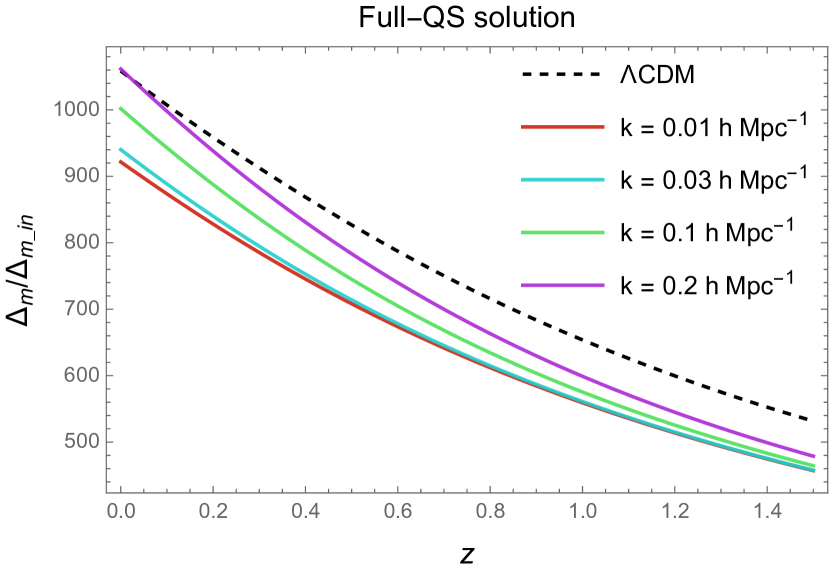
Little scale dependence is observed across all the relevant modes for the full covariant and semi QS methods at low redshifts. The scale dependence is more pronounced for the full QS method.
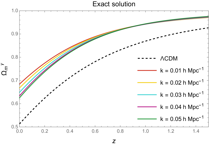
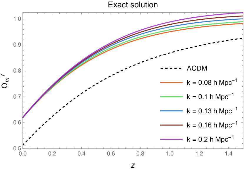
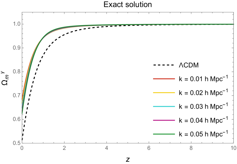
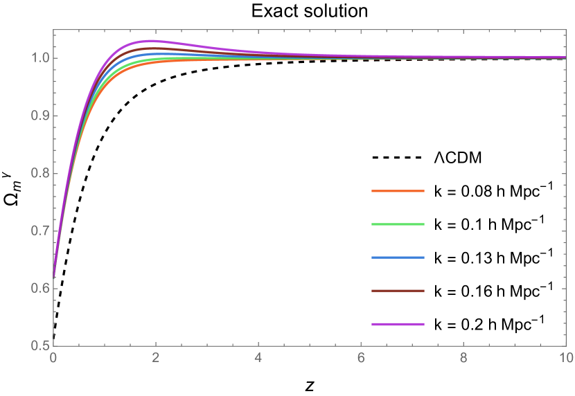
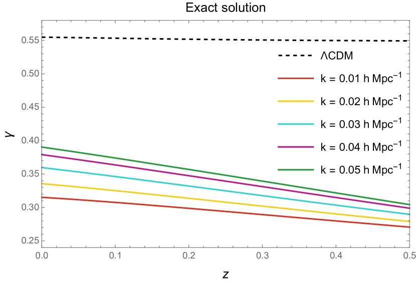
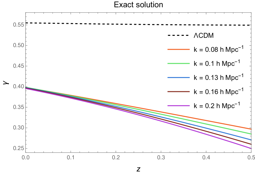
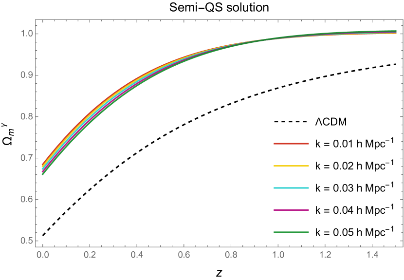
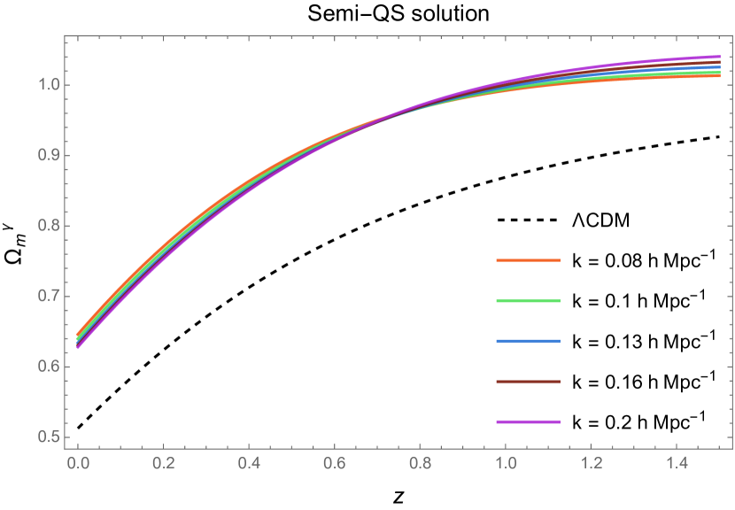
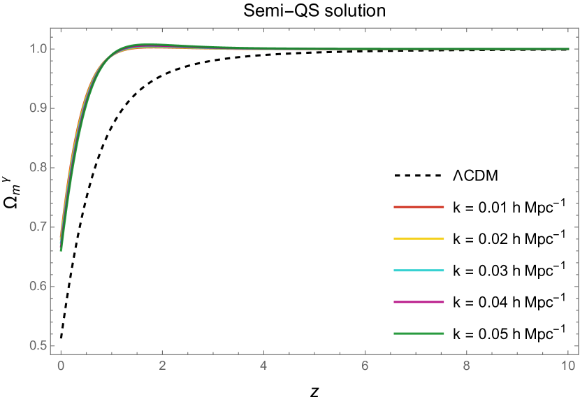
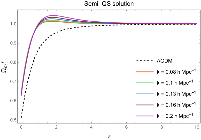
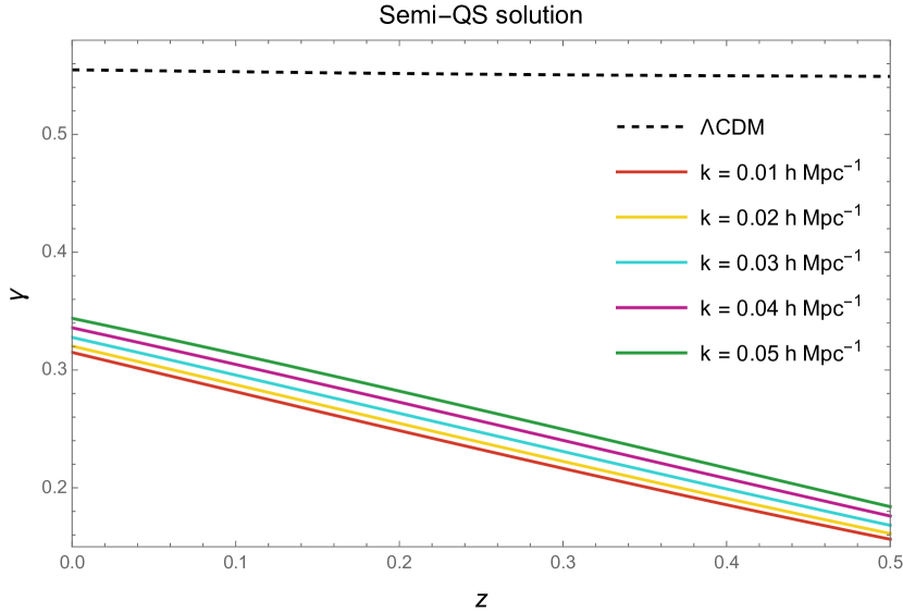
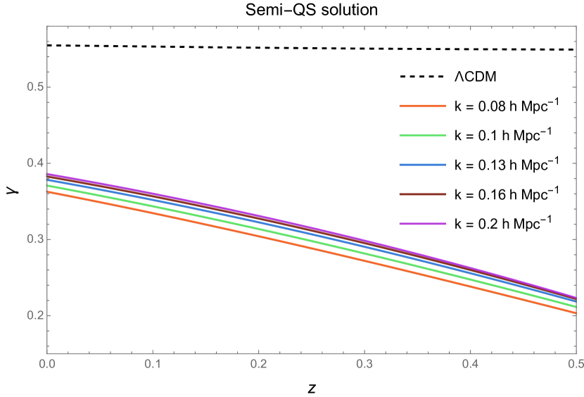
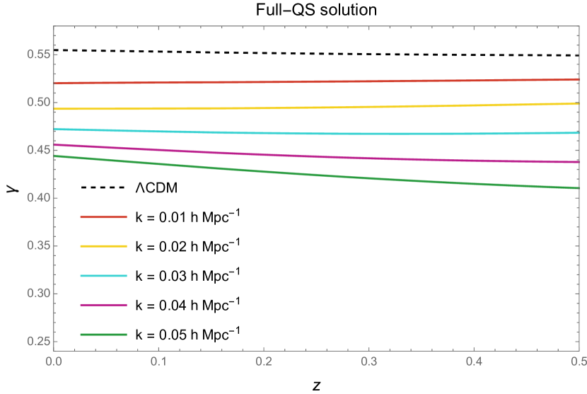
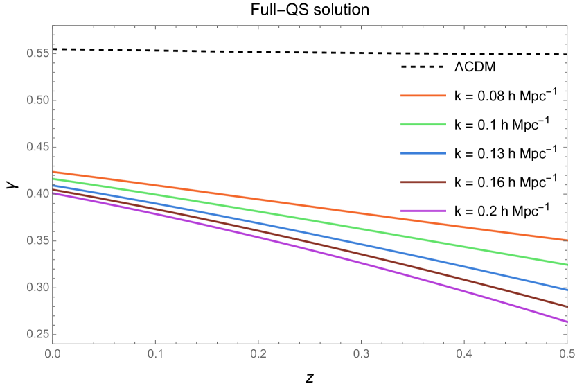
The growth rate function defined in Eq.(40) and the growth index parameter defined in Eq.(41) associated with the full covariant, semi QS and full QS perturbation method are shown in Figs 10, 11, and 12 respectively. Here the scales are split for each method to show general large vs small scale trends. All methods show similar results for smaller scales (right columns), with the scale dependence of being only minor at and becoming more pronounced at around . From Fig 6, it is apparent that all of these scales have been in the regime since and have thus had time to feel the effect of the fifth force, leading to significant deviation from CDM. For larger scales (left columns), the trend is inverted with scale-dependence being much larger at . From Fig 12, we see that the growth function and growth index for the full QS method differ significantly from the other methods and, in the case of the growth function, only marginally from CDM. For the growth index, while the values of are not exactly those found for CDM, the suppression of is far weaker and the growth is far slower than in the methods. This again emphasises the inability to distinguish from CDM at these scales using the full QS method.
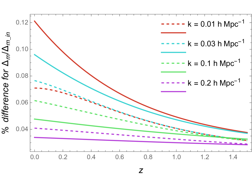
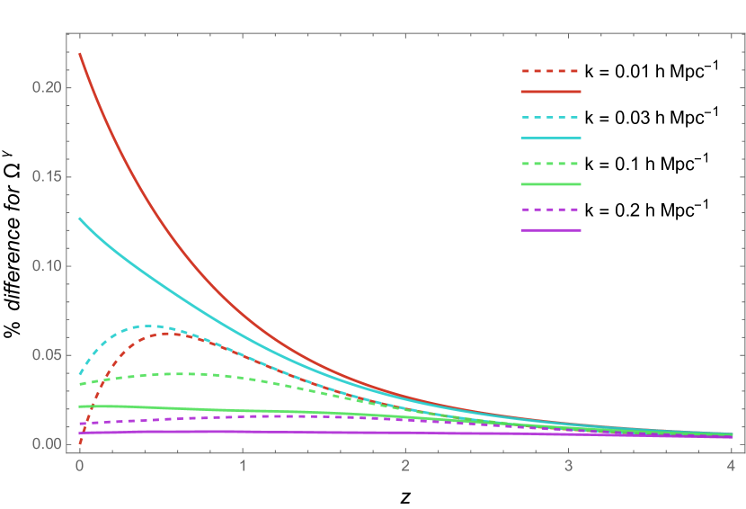
The differences between methods are examined in a more quantitative manner in Fig. 13, where the percentage differences between the exact solution and both the semi QS and full QS solutions are plotted for both large and small scales. Two general trends that are observed are the following
-
•
The difference between the solutions obtained with QS approximations (semi or full) and the exact solutions are larger for larger scales and smaller for smaller scales.
-
•
For smaller scales, solutions with full QS approximation appear closer to the exact solutions than solutions with semi QS approximation. The opposite is true for larger scales.
This scale-dependent behavior is evidently an important factor to take into account when applying the QS approximation in gravity.
Despite differences across methods at different scales, the results are in general in agreement with various model-specific or constrained structure analyses Huterer et al. (2015); Narikawa & Yamamoto (2010); Mirzatuny & Pierpaoli (2019); Motohashi et al. (2011); Polarski & Gannouji (2008); Gannouji et al. (2009); Tsujikawa (2010). They display clear scale dependence, which becomes more pronounced at smaller scales, along with larger growth rate and significant deviation from CDM for the growth index on small redshifts.
Further emphasising the difference from CDM, there is clear time-dependence for displayed on even small redshifts. models are known to admit a growth index of this form, often approximated as
| (70) |
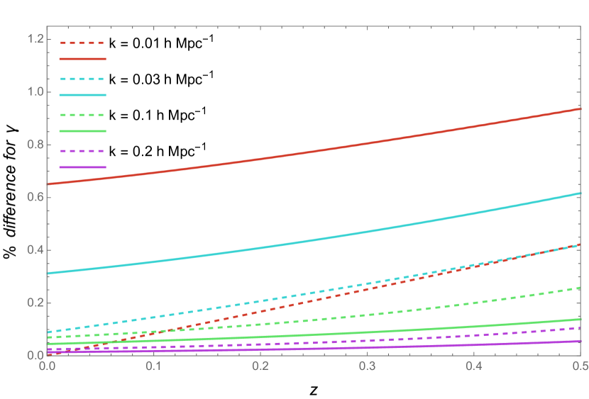
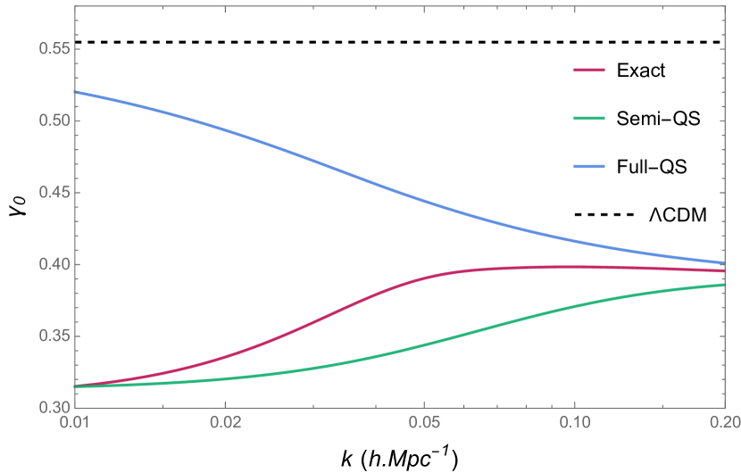
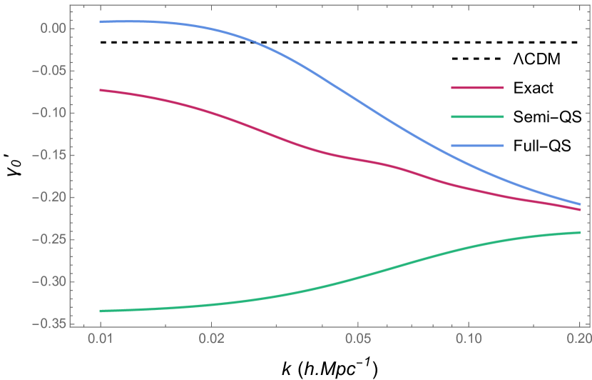
for low redshifts. Both and can be inferred from a number of observables, including rich clusters, redshift space distortions and tomographic weak lensing (see Reid et al. (2015); Planck Collaboration et al. (2020); Amendola et al. (2008); Thomas et al. (2009); Belloso et al. (2011); Pouri et al. (2014)), however current constraints are not tight enough to definitively rule out a number of DE and modified gravity models. As a means of direct comparison with previous model-dependent analysis, the scale dependence of and for each method is shown in Fig 14.
All three methods come close to converging for both and for , as these are scales where both of the QS approximations are relevant. Again, we see in Fig 14(a) that only applying the semi QS approximation drives the value of further from the values of both the full QS and exact solutions for small scales, while for the largest scales this approximation for matches the exact solution. The full QS solutions at large scales show a value for much closer to that of CDM, validating the notion that this approximation is insufficient for distinguishing between and CDM at these scales. However, this is markedly different when looking at in Fig 14(b) where, on all scales, the semi QS method shows more significant deviation from the exact solution than the full QS method.
Confining our view to only the exact solutions for simplicity, we see that these model-independent results are in agreement with previous model-dependent analyses, giving and Polarski & Gannouji (2008); Gannouji et al. (2009); Tsujikawa (2010); Tsujikawa et al. (2009); Narikawa & Yamamoto (2010). Regardless of marginal differences between methods, there is a dispersion across scales of at least for both and . This would be a strong indication of modified gravity if detected in sufficiently sensitive observations.
9 Discussion and Conclusion
In this paper, we extend our model-independent, cosmography-based approach to studying cosmologies which mimic CDM Chakraborty et al. (2021) to include analysis of the growth factor. To the best of our knowledge, this is the first time this type of analysis has been performed in a model-independent manner, i.e., without a-priori specifying the functional form of . This is achieved by recasting the terms involving and its derivatives in terms of the cosmographic parameters (), which appear in the 1+3 covariant perturbation equations. We begin by reviewing the background model-independent analysis and emphasising the power of cosmography to describe the evolution of the cosmological expansion history. We then reformulate the exact linear perturbation equations and employ the separate quasi-static assumptions, leading to the semi and full quasi-static approximation equations. We explore the cosmographic condition and use this to specify a cosmic evolution that mimics the CDM evolution at the background level. Then, we consider the dynamics of matter perturbation using the 1+3 covariant gauge-invariant formalism. Finally, we examine the evolution of the growth rate function and the growth index parameter for different scales at the levels of exact, semi and full quasi-static approximations and compare them with the model-specific trends. We also show the dispersion across scales of the growth index parameter, which is a characteristic of modified gravity theories.
From these results we found that our approach (both with and without quasi-static approximations) is capable of capturing in a totally general way features that have earlier been observed in various earlier model-specific or constrained structure analyses Polarski & Gannouji (2008); Gannouji et al. (2009); Fonseca et al. (2019). The density contrast , growth function and growth index display clear scale-dependence, which becomes more pronounced on smaller scales for redshift . Additionally, exhibits strong time-dependence and significantly smaller values, representing a substantial deviation from the CDM model. A major achievement of our approach is the ability to obtain information about the present day values of the growth index and its derivative, and , for CDM-mimicking models without needing to specify any particular theory. As explicitly reconstructed forms of which mimic CDM tend to be hypergeometric functions Dunsby et al. (2010); He & Wang (2013), calculating these quantities and their dispersion would have been extremely complex without our approach.
Finally, by comparing the exact, semi and full quasi-static methods, we were able to determine the shortcomings of the full QS method on large scales, where the perturbations have not spent significant time in the regime and are thus trend closer to CDM. For this reason, we caution against using the full quasi-static approximation for scales h.Mpc-1. For smaller scales, the differences between these methods are marginal. Regardless of the method, these results provide strong support and confirmation of many structure growth studies, while avoiding both the need to narrow the analysis by choosing a form of and the great complexity that results from the reconstruction programme. Even with the consideration of the exact perturbation equations (i.e. without any approximation), our approach is relatively uncomplicated, computationally simple and allows us to determine predictions that can be tested with accurate data from future weak lensing surveys. The approach can also be easily implemented for other modifications of gravity and dynamical dark energy models, as well as background expansion histories which differ from CDM.
10 Acknowledgements
KM thanks the University of Cape Town for financial assistance. SC acknowledges funding support from the NSRF via the Program Management Unit for Human Resources and Institutional Development, Research and Innovation (Thailand) [grant number B13F670063]. JW thanks the National Astrophysics and Space Science Programme and the University of Cape Town for their financial support. PKSD thanks the First Rand Bank for financial support.
References
- Abdelwahab et al. (2012) Abdelwahab M., Goswami R., Dunsby P. K. S., 2012, Phys. Rev. D, 85, 083511
- Abebe et al. (2013) Abebe A., de la Cruz-Dombriz A., Dunsby P. K. S., 2013, Phys. Rev. D, 88, 044050
- Adler et al. (1995) Adler R. J., Casey B., Jacob O. C., 1995, American Journal of Physics, 63, 620
- Amendola et al. (2008) Amendola L., Kunz M., Sapone D., 2008, Journal of Cosmology and Astroparticle Physics, 2008, 013
- Amirhashchi & Amirhashchi (2020) Amirhashchi H., Amirhashchi S., 2020, Gen. Rel. Grav., 52, 13
- Ananda et al. (2009) Ananda K. N., Carloni S., Dunsby P. K. S., 2009, Classical and Quantum Gravity, 26, 235018
- Bean et al. (2007) Bean R., Bernat D., Pogosian L., Silvestri A., Trodden M., 2007, Physical Review D, 75
- Belloso et al. (2011) Belloso A. B., García-Bellido J., Sapone D., 2011, Journal of Cosmology and Astroparticle Physics, 2011, 010
- Blumenthal et al. (1984) Blumenthal G. R., Faber S. M., Primack J. R., Rees M. J., 1984, Nature, 311, 517
- Bolotin et al. (2018) Bolotin Y. L., Cherkaskiy V. A., Ivashtenko O. Y., Konchatnyi M. I., Zazunov L. G., 2018, arXiv e-prints
- Bruni et al. (1992) Bruni M., Ellis G. F. R., Dunsby P. K. S., 1992, Classical and Quantum Gravity, 9, 921
- Capozziello & Francaviglia (2008) Capozziello S., Francaviglia M., 2008, Gen. Rel. Grav., 40, 357
- Capozziello et al. (2008) Capozziello S., Cardone V. F., Salzano V., 2008, Phys. Rev. D, 78, 063504
- Carloni (2015) Carloni S., 2015, Journal of Cosmology and Astroparticle Physics, 2015, 013
- Carloni & Dunsby (2007) Carloni S., Dunsby P. K. S., 2007, J. Phys. A, 40, 6919
- Carloni et al. (2005) Carloni S., Dunsby P. K. S., Capozziello S., Troisi A., 2005, Class. Quant. Grav., 22, 4839
- Carloni et al. (2008) Carloni S., Dunsby P. K. S., Troisi A., 2008, Phys. Rev. D, 77, 024024
- Carloni et al. (2009) Carloni S., Troisi A., Dunsby P. K. S., 2009, Gen. Rel. Grav., 41, 1757
- Carloni et al. (2012) Carloni S., Goswami R., Dunsby P. K. S., 2012, Class. Quant. Grav., 29, 135012
- Carroll et al. (2004) Carroll S. M., Duvvuri V., Trodden M., Turner M. S., 2004, Phys. Rev. D, 70, 043528
- Chakraborty et al. (2021) Chakraborty S., MacDevette K., Dunsby P., 2021, Phys. Rev. D, 103, 124040
- Chakraborty et al. (2023) Chakraborty S., Gregoris D., Mishra B., 2023, Phys. Lett. B, 842, 137962
- De Felice & Tsujikawa (2010) De Felice A., Tsujikawa S., 2010, Living Rev. Rel., 13, 3
- De la Cruz-Dombriz et al. (2008) De la Cruz-Dombriz A., Dobado A., Maroto A. L., 2008, Physical Review D, 77
- Dicke (1961) Dicke R. H., 1961, Nature, 192, 440
- Dunajski & Gibbons (2008) Dunajski M., Gibbons G., 2008, Class. Quant. Grav., 25, 235012
- Dunsby & Luongo (2016) Dunsby P. K. S., Luongo O., 2016, Int. J. Geom. Meth. Mod. Phys., 13, 1630002
- Dunsby et al. (1992) Dunsby P. K., Bruni M., Ellis G. F., 1992, Astrophysical Journal, Part 1 (ISSN 0004-637X), vol. 395, no. 1, p. 54-74., 395, 54
- Dunsby et al. (2010) Dunsby P. K. S., Elizalde E., Goswami R., Odintsov S., Gomez D. S., 2010, Phys. Rev. D, 82, 023519
- Ellis & Bruni (1989) Ellis G. F. R., Bruni M., 1989, Phys. Rev. D, 40, 1804
- Fonseca et al. (2019) Fonseca J., Viljoen J.-A., Maartens R., 2019, Journal of Cosmology and Astroparticle Physics, 2019, 028
- Gannouji & Polarski (2008) Gannouji R., Polarski D., 2008, Journal of Cosmology and Astroparticle Physics, 2008, 018
- Gannouji et al. (2009) Gannouji R., Moraes B., Polarski D., 2009, Journal of Cosmology and Astroparticle Physics, 2009, 034
- He & Wang (2013) He J.-h., Wang B., 2013, Phys. Rev. D, 87, 023508
- Hojjati et al. (2012) Hojjati A., Pogosian L., Silvestri A., Talbot S., 2012, Phys. Rev. D, 86, 123503
- Huterer et al. (2015) Huterer D., et al., 2015, Astroparticle Physics, 63, 23
- Kinney (2002) Kinney W. H., 2002, Phys. Rev. D, 66, 083508
- Liddle (2003) Liddle A. R., 2003, Phys. Rev. D, 68, 103504
- Lightman & Schechter (1990) Lightman A. P., Schechter P. L., 1990, ApJS, 74, 831
- Mehrabi & Rezaei (2021) Mehrabi A., Rezaei M., 2021, Astrophys. J., 923, 274
- Mirzatuny & Pierpaoli (2019) Mirzatuny N., Pierpaoli E., 2019, Journal of Cosmology and Astroparticle Physics, 2019, 066
- Motohashi et al. (2011) Motohashi H., Starobinsky A. A., Yokoyama J., 2011, International Journal of Modern Physics D, 20, 1347
- Mukherjee & Banerjee (2016) Mukherjee A., Banerjee N., 2016, Phys. Rev. D, 93, 043002
- Mukherjee & Banerjee (2017) Mukherjee A., Banerjee N., 2017, Class. Quant. Grav., 34, 035016
- Mukherjee & Banerjee (2021) Mukherjee P., Banerjee N., 2021, Eur. Phys. J. C, 81, 36
- Narikawa & Yamamoto (2009) Narikawa T., Yamamoto K., 2009, in 19th Workshop on General Relativity and Gravitation in Japan.
- Narikawa & Yamamoto (2010) Narikawa T., Yamamoto K., 2010, Phys. Rev. D, 81, 043528
- Nojiri et al. (2009) Nojiri S., Odintsov S. D., Saez-Gomez D., 2009, Phys. Lett. B, 681, 74
- Noller et al. (2014) Noller J., von Braun-Bates F., Ferreira P. G., 2014, Phys. Rev. D, 89, 023521
- Ostriker & Steinhardt (1995) Ostriker J. P., Steinhardt P. J., 1995, arXiv e-prints, pp astro–ph/9505066
- Peebles (1980) Peebles P. J. E., 1980, The large-scale structure of the universe
- Planck Collaboration et al. (2020) Planck Collaboration et al., 2020, A&A, 641, A6
- Pogosian & Silvestri (2008) Pogosian L., Silvestri A., 2008, Phys. Rev. D, 77, 023503
- Polarski & Gannouji (2008) Polarski D., Gannouji R., 2008, Physics Letters B, 660, 439
- Pouri et al. (2014) Pouri A., Basilakos S., Plionis M., 2014, Journal of Cosmology and Astroparticle Physics, 2014, 042
- Reid et al. (2015) Reid B., et al., 2015, Monthly Notices of the Royal Astronomical Society, 455, 1553
- Sahni et al. (2003) Sahni V., Saini T. D., Starobinsky A. A., Alam U., 2003, JETP Lett., 77, 201
- Sawicki & Bellini (2015) Sawicki I., Bellini E., 2015, Phys. Rev. D, 92, 084061
- Silvestri et al. (2013) Silvestri A., Pogosian L., Buniy R. V., 2013, Phys. Rev. D, 87, 104015
- Sotiriou & Faraoni (2010) Sotiriou T. P., Faraoni V., 2010, Rev. Mod. Phys., 82, 451
- Spalinski (2007) Spalinski M., 2007, JCAP, 08, 016
- Steinhardt (1998) Steinhardt P. J., 1998, 7 COSMOLOGICAL CHALLENGES FOR THE 21ST CENTURY. Princeton University Press, Princeton, pp 123–146, doi:doi:10.1515/9780691227498-008
- Stelle (1978) Stelle K. S., 1978, Gen. Rel. Grav., 9, 353
- Tada & Terada (2024) Tada Y., Terada T., 2024, Phys. Rev. D, 109, L121305
- Thomas et al. (2009) Thomas S. A., Abdalla F. B., Weller J., 2009, Monthly Notices of the Royal Astronomical Society, 395, 197
- Tsujikawa (2007) Tsujikawa S., 2007, Phys. Rev. D, 76, 023514
- Tsujikawa (2010) Tsujikawa S., 2010, Modified Gravity Models of Dark Energy. Springer Berlin Heidelberg, Berlin, Heidelberg, pp 99–145, doi:10.1007/978-3-642-10598-2_3
- Tsujikawa et al. (2009) Tsujikawa S., Gannouji R., Moraes B., Polarski D., 2009, Phys. Rev. D, 80, 084044
- Zhai et al. (2013) Zhai Z.-X., Zhang M.-J., Zhang Z.-S., Liu X.-M., Zhang T.-J., 2013, Phys. Lett. B, 727, 8