Thermal quasi-particle theory

Abstract

The widely used thermal Hartree–Fock (HF) theory is generalized to include the effect of electron correlation while maintaining its quasi-independent-particle framework. An electron-correlated internal energy (or grand potential) is postulated in consultation with the second-order finite-temperature many-body perturbation theory (MBPT), which then dictates the corresponding thermal orbital (quasi-particle) energies in such a way that all fundamental thermodynamic relations are obeyed. The associated density matrix is of a one-electron type, whose diagonal elements take the form of the Fermi–Dirac distribution functions, when the grand potential is minimized. The formulas for the entropy and chemical potential are unchanged from those of Fermi–Dirac or thermal HF theory. The theory thus constitutes a finite-temperature extension of the second-order Dyson self-energy of one-particle many-body Green’s function theory and can be viewed as a second-order, diagonal, frequency-independent, thermal inverse Dyson equation. At low temperature, the theory approaches finite-temperature MBPT of the same order, but it may outperform the latter at intermediate temperature by including additional electron-correlation effects through orbital energies. A physical meaning of these thermal orbital energies is proposed (encompassing that of thermal HF orbital energies, which has been elusive) as a finite-temperature version of Janak’s theorem.

I Introduction

Thermal Hartree–Fock (HF) theoryHusimi (1940); Mermin (1963); Gu and Hirata (2024) is a curious ansatz. It uses an auxiliary one-electron Hamiltonian to define its one-electron density matrix, whereas a true density matrix for thermodynamics governed by an interacting Hamiltonian should be much higher ranked.Farid, March, and Theophilou (2000) Its diagonal elements, as variational parameters, ultimately become the Fermi–Dirac distribution functions of the non-interacting Fermi–Dirac theory, when the grand potential is minimized. The state energies defining this grand potential are, however, evaluated with the exact Hamiltonian containing two-electron interactions. Stipulated in this way, the theory does not seem to correspond to a single, consistent grand partition function.

Nevertheless, the thermodynamic functions of this theory are shownArgyres, Kaplan, and Silva (1974); Gu and Hirata (2024) to obey all fundamental thermodynamic relations. They also correctly reduceGu and Hirata (2024) to the zero-temperature HF theory.Szabo and Ostlund (1982); Shavitt and Bartlett (2009) They are widely used in applications to, e.g., energy bands in a solid where their temperature-dependent orbital energies are often invoked, somewhat unquestioningly, in explaining metal-insulator transitions,Hermes and Hirata (2015) etc. This is in spite of the facts that their physical meaning is still obscurePain (2011) and that state energies in quantum mechanics are supposed to be constant of temperature.

In this article, inspired by the immense success of thermal HF theory, we generalize this ansatz to include the effects of electron correlation, while keeping to its quasi-independent-particle framework and grand canonical ensemble. Such a theory, which can provide electron-correlated (i.e., quasi-particle) energy bands of semiconductors at finite temperatures in addition to their thermodynamic functions, may prove even more useful than thermal HF theory or thermal density-functional theory (DFT). Our strategy of postulating what we call thermal quasi-particle theory is as follows:

We first assume that every state consists of non-interacting quasi-particles, each occupying a well-defined orbital with an electron-correlated orbital energy. An internal energy (or grand potential) is postulated by consulting with finite-temperature many-body perturbation theory (MBPT).Hirata and Jha (2019, 2020); Hirata (2021a) Its definition dictates the forms of the thermal quasi-particle energies (i.e., the electron-correlated thermal orbital energies) such that all fundamental thermodynamic relations are obeyed. The corresponding density matrix is then of a one-electron type, whose diagonal elements take the form of the Fermi–Dirac distribution functions, when the grand potential is minimized. The formulas for the entropy and average number of electrons (determining the chemical potential) are unchanged from the corresponding formulas of Fermi–Dirac or thermal HF theory. The thermal quasi-particle energies thus defined are a finite-temperature generalizationMatsubara (1955); Luttinger and Ward (1960); March, Young, and Sampanthar (1967); Kadanoff and Baym (2018) of the Dyson self-energies of one-particle many-body Green’s function (MBGF) theory.Linderberg and Öhrn (1973); Paldus and Čížek (1975); Cederbaum and Domcke (1977); Simons (1977); Öhrn and Born (1981); Jørgensen and Simons (1981); Oddershede (1987); Aryasetiawan and Gunnarsson (1998); Ortiz (1999); Onida, Reining, and Rubio (2002); Ortiz (2013); Hirata et al. (2017, 2024)

Being based on perturbation theory, thermal quasi-particle theory forms a hierarchy of size-consistentHirata (2011) approximations with increasing accuracy and complexity. Fermi–Dirac and thermal HF theories can be viewed, respectively, as the zeroth- and first-order instances of this hierarchy. Here, we introduce a second-order thermal quasi-particle theory, which is the leading order in describing electron correlation. It is based on the second-order grand potential or internal energy of finite-temperature MBPT.Hirata and Jha (2020); Hirata (2021a) We propose the expression for the corresponding second-order thermal self-energies, which obey all thermodynamic relations and ensure the variationality of the grand potential. The theory thus constitutes a second-order, diagonal, frequency-independent, thermal inverse Dyson equation.Hirata et al. (2017) It reduces to the second-order MBPT for internal energy and to the second-order MBGF (in the diagonal and frequency-independent approximation) for orbital energies at zero temperature.

A comparison of thermal quasi-particle theories with finite-temperature MBPT suggests that the former may include higher-order perturbation corrections through correlation-corrected thermal orbital energies and outperform the latter at intermediate temperature. We also propose a physical meaning of these thermal orbital energies in the form of a finite-temperature version of Janak’s theorem.Janak (1978) It encompasses the physical meaning of thermal HF orbital energies, which has been elusive.Pain (2011); Hirata (2021a)

II Thermal quasi-particle theory

II.1 Zeroth order

Fermi–Dirac theory is the zeroth-order thermal quasi-particle theory [thermal QP(0) theory]. It is reviewed briefly to outline the general framework of the hierarchical approximations; it is discussed more fully in Ref. Gu and Hirata, 2024.

Its internal energy $U^{(0)}$ and entropy $S^{(0)}$ at the inverse temperature $\beta=(k_{\text{B}}T)^{-1}$ are given by

$$U^{(0)} \equiv \langle E^{(0)}\rangle=\sum_{p}\epsilon_{p}^{(0)}f_{p}^{-},$$ (1)

$$S^{(0)} \equiv -k_{\text{B}}\left(f_{p}^{-}\ln f_{p}^{-}+f_{p}^{+}\ln f_{p}^{+}\right)$$ (2)

with the Fermi–Dirac distribution functions,

$$f_{p}^{-} = \frac{1}{1+e^{\beta(\epsilon_{p}^{(0)}-\mu^{(0)})}},$$ (3)

$$f_{p}^{+} = 1-f_{p}^{-}=\frac{e^{\beta(\epsilon_{p}^{(0)}-\mu^{(0)})}}{1+e^{\beta(\epsilon_{p}^{(0)}-\mu^{(0)})}}.$$ (4)

Here, $\epsilon_{p}^{(0)}$ is the energy of the $p$th spinorbital of a reference wave function, and $\mu^{(0)}$ is the chemical potential determined by the electroneutrality condition,

$$\bar{N} = \sum_{p}f_{p}^{-},$$ (5)

where $\bar{N}$ is the average number of electrons that cancel nuclear charges exactly, and the summations are always taken over all spinorbitals.

The $\langle E^{(n)}\rangle$ in Eq. (1) is a zeroth-order thermal average of state energies, i.e.,

$$\langle E^{(n)}\rangle \equiv \frac{\sum_{I}E_{I}^{(n)}e^{-\beta(E_{I}^{(0)}-\mu^{(0)}N_{I})}}{\sum_{I}e^{-\beta(E_{I}^{(0)}-\mu^{(0)}N_{I})}},$$ (6)

where $E_{I}^{(n)}$ is the $n$th-order perturbation correction to the energy of the $I$th Slater-determinant state according to Hirschfelder–Certain degenerate perturbation theory,Hirschfelder and Certain (1974) and $E_{I}^{(0)}=\sum\epsilon_{i}^{(0)}$ ($i$ labels spinorbitals occupied in the $I$th state). Sum-over-states expressions of the thermal averages can be reduced to sum-over-orbitals ones either by combinatorial logicHirata and Jha (2019, 2020) or by normal-ordered second quantization at finite temperature.Hirata (2021a)

The grand potential $\Omega^{(0)}$ is then given by

$$\Omega^{(0)} \equiv U^{(0)}-\mu^{(0)}\bar{N}-TS^{(0)}$$

$$= \sum_{p}\left(\epsilon_{p}^{(0)}-\mu^{(0)}\right)f_{p}^{-}+\frac{1}{\beta}\sum_{p}\left(f_{p}^{-}\ln f_{p}^{-}+f_{p}^{+}\ln f_{p}^{+}\right).$$

As explicitly shown in Ref. Gu and Hirata, 2024, they satisfy the thermodynamic relations such as Eq. (II.1) and

$$-\frac{\partial\Omega^{(0)}}{\partial\mu^{(0)}} = \bar{N},$$ (9)

$$-\frac{\partial\Omega^{(0)}}{\partial T} = S^{(0)}.$$ (10)

The Fermi–Dirac distribution function [Eq. (3)] is a diagonal element of the one-electron density matrix that minimizes the grand potential. Therefore,

$$\frac{\partial\Omega^{(0)}}{\partial f_{p}^{-}} = 0,$$ (11)

which is also explicitly verifiable.Gu and Hirata (2024)

Fermi–Dirac theory is an exact theory for thermodynamics of a system governed by an independent-particle Hamiltonian.

II.2 First order

Thermal HF theoryHusimi (1940); Mermin (1963) constitutes the first-order thermal quasi-particle theory [thermal QP(1) theory]. It is also fully discussed in Ref. Gu and Hirata, 2024. It accommodates the exact Hamiltonian with two-electron interactions within a quasi-independent-particle framework.

Its internal energy $U^{\text{HF}}$ is postulated by an intuitively natural finite-temperature generalization of the zero-temperature HF energy,Hirata (2021a) i.e.,

$$U^{\text{HF}} \equiv \langle E^{(0)}\rangle+\langle E^{(1)}\rangle$$ (12)

$$= \sum_{p}\epsilon_{p}^{\text{HF}}f_{p}^{-}-\frac{1}{2}\sum_{p,q}\langle pq||pq\rangle f_{p}^{-}f_{q}^{-}$$ (13)

with

$$\epsilon_{p}^{\text{HF}} \equiv h_{pp}+\sum_{r}\langle pr||pr\rangle f_{r}^{-},$$ (14)

where $h_{pq}$ is the one-electron (“core”) part of the Hamiltonian matrix element,Szabo and Ostlund (1982) $\langle pq||rs\rangle$ is an anti-symmetrized two-electron integral,Szabo and Ostlund (1982); Shavitt and Bartlett (2009) and $\langle E^{(1)}\rangle$ has been reduced in Eqs. (45) and (46) of Ref. Hirata and Jha, 2020. Spinorbitals labeled by $p$ and $q$ are the ones that bring the matrix of thermal HF orbital energies $\bm{\epsilon}^{\text{HF}}$ into a diagonal form, i.e.,

$$\epsilon_{pq}^{\text{HF}} = h_{pq}+\sum_{r}\langle pr||qr\rangle f_{r}^{-}=\delta_{pq}\epsilon_{p}^{\text{HF}},$$ (15)

where $\delta_{pq}$ is Kronecker’s delta.

The Fermi–Dirac distribution functions,

$$f_{p}^{-} = \frac{1}{1+e^{\beta(\epsilon_{p}^{\text{HF}}-\mu^{\text{HF}})}},$$ (16)

$$f_{p}^{+} = 1-f_{p}^{-}=\frac{e^{\beta(\epsilon_{p}^{\text{HF}}-\mu^{\text{HF}})}}{1+e^{\beta(\epsilon_{p}^{\text{HF}}-\mu^{\text{HF}})}},$$ (17)

are now defined with $\epsilon_{p}^{\text{HF}}$ and $\mu^{\text{HF}}$. The latter is determined by the same electroneutrality condition,

$$\bar{N} = \sum_{p}f_{p}^{-}.$$ (18)

The entropy formula is unchanged from that of Fermi–Dirac theory [Eq. (2)],

$$S^{\text{HF}} \equiv -k_{\text{B}}\sum_{p}\left(f_{p}^{-}\ln f_{p}^{-}+f_{p}^{+}\ln f_{p}^{+}\right).$$ (19)

The grand potential is therefore given by

$$\Omega^{\text{HF}} \equiv U^{\text{HF}}-\mu^{\text{HF}}\bar{N}-TS^{\text{HF}}$$ (21)

$$= \sum_{p}\left(\epsilon_{p}^{\text{HF}}-\mu^{\text{HF}}\right)f_{p}^{-}-\frac{1}{2}\sum_{p,q}\langle pq||pq\rangle f_{p}^{-}f_{q}^{-}$$

$$+\frac{1}{\beta}\sum_{p}\left(f_{p}^{-}\ln f_{p}^{-}+f_{p}^{+}\ln f_{p}^{+}\right).$$

These thermodynamic functions together satisfyGu and Hirata (2024) the thermodynamic relations such as Eq. (21) by construction as well as

$$-\frac{\partial\Omega^{\text{HF}}}{\partial\mu^{\text{HF}}} = \bar{N},$$ (22)

$$-\frac{\partial\Omega^{\text{HF}}}{\partial T} = S^{\text{HF}},$$ (23)

$$\frac{\partial\Omega^{\text{HF}}}{\partial f_{p}^{-}} = 0.$$ (24)

The last identity underscores that $\Omega^{\text{HF}}$ is minimizedMermin (1963); Gu and Hirata (2024) by the orbitals that diagonalize $\bm{\epsilon}^{\text{HF}}$ [Eq. (15)] and by the one-particle density matrix whose eigenvalues are the Fermi–Dirac distribution functions of Eq. (16).

II.3 Second order

We postulate a second-order thermal quasi-particle theory [thermal QP(2) theory] by its internal energy,

$$U^{\text{QP(2)}} \equiv \langle E^{(0)}\rangle+\langle E^{(1)}\rangle+\langle E^{(2)}\rangle.$$ (25)

The last term $\langle E^{(2)}\rangle$ is the thermal average of second-order Hirschfelder–Certain degenerate perturbation energiesHirschfelder and Certain (1974) and has been reduced in Eqs. (C7) and (C8) of Ref. Hirata and Jha, 2020 to the following sum-over-orbitals formula:

$$\langle E^{(2)}\rangle = \sum_{p,q}^{\text{denom.}\neq 0}\frac{F_{qp}F_{pq}}{\epsilon_{p}^{(0)}-\epsilon_{q}^{(0)}}f_{p}^{-}f_{q}^{+}$$

$$+\frac{1}{4}\sum_{p,q,r,s}^{\text{denom.}\neq 0}\frac{\langle pq||rs\rangle\langle rs||pq\rangle}{\epsilon_{p}^{(0)}+\epsilon_{q}^{(0)}-\epsilon_{r}^{(0)}-\epsilon_{s}^{(0)}}f_{p}^{-}f_{q}^{-}f_{r}^{+}f_{s}^{+}$$

with

$$F_{pq}\equiv\epsilon_{pq}^{\text{HF}}-\delta_{pq}\epsilon_{p}^{(0)},$$ (27)

where “denom.$\neq 0$” restricts the summation to over those indexes whose denominator is nonzero.Hirata and Jha (2020); Hirata (2021a)

It is a natural finite-temperature generalization of second-order many-body perturbation energy,Bartlett (1981); Shavitt and Bartlett (2009) but is considerably simpler than the full second-order correction to the internal energy $U^{(2)}$ of finite-temperature MBPT [Eq. (74) of Ref. Hirata and Jha, 2020]. The simplification is at least partly justified by the equally simpler treatments of the chemical-potential and entropy contributions to adhere to the quasi-independent-particle framework that the theory adopts.

The first term of $\langle E^{(2)}\rangle$ [Eq. (LABEL:E2)] is the so-called non-HF term (or more precisely, non-thermal-HF term, in this case),Shavitt and Bartlett (2009) which is zero when thermal HF theory is used as the reference (where $F_{pq}=0$). The diagrammatic representationHirata (2021a) of $\langle E^{(2)}\rangle$ is given in Fig. 1.

Figure 1: Shavitt–Bartlett-style diagramsShavitt and Bartlett (2009); Hirata (2021a) of $\langle E^{(2)}\rangle$ of Eq. (LABEL:E2). Each downgoing (upgoing) edge represents $f_{p}^{-}$ ($f_{p}^{+}$), a dashed line is an anti-symmetrized two-electron integral, a dashed line with a circle denotes $F_{pq}$, and a wiggly (resolvent) line is a denominator factor.

We thus have

$$U^{\text{QP(2)}} \equiv \sum_{p}\epsilon_{p}^{\text{HF}}f_{p}^{-}-\frac{1}{2}\sum_{p,q}\langle pq||pq\rangle f_{p}^{-}f_{q}^{-}$$

$$+\sum_{p,q}^{\text{denom.}\neq 0}\frac{F_{qp}F_{pq}}{\epsilon_{p}^{(0)}-\epsilon_{q}^{(0)}}f_{p}^{-}f_{q}^{+}$$

$$+\frac{1}{4}\sum_{p,q,r,s}^{\text{denom.}\neq 0}\frac{\langle pq||rs\rangle\langle rs||pq\rangle}{\epsilon_{p}^{(0)}+\epsilon_{q}^{(0)}-\epsilon_{r}^{(0)}-\epsilon_{s}^{(0)}}f_{p}^{-}f_{q}^{-}f_{r}^{+}f_{s}^{+}.$$

The entropy formula retains the one-particle picture and takes the form,

$$S^{\text{QP(2)}} \equiv -k_{\text{B}}\sum_{p}\left(f_{p}^{-}\ln f_{p}^{-}+f_{p}^{+}\ln f_{p}^{+}\right),$$ (29)

which differs materially from the $S^{(0)}+S^{(1)}+S^{(2)}$ of Refs. Hirata and Jha, 2020; Hirata, 2021a, but is more in line with thermal HF or Fermi–Dirac theory. The corresponding grand potential is then defined by

$$\Omega^{\text{QP(2)}} \equiv U^{\text{QP(2)}}-\mu^{\text{QP(2)}}\bar{N}-TS^{\text{QP(2)}}$$ (31)

$$= \sum_{p}\left(\epsilon_{p}^{\text{HF}}-\mu^{\text{QP(2)}}\right)f_{p}^{-}-\frac{1}{2}\sum_{p,q}\langle pq||pq\rangle f_{p}^{-}f_{q}^{-}$$

$$+\frac{1}{\beta}\sum_{p}\left(f_{p}^{-}\ln f_{p}^{-}+f_{p}^{+}\ln f_{p}^{+}\right)+\langle E^{(2)}\rangle,$$

where $\mu^{\text{QP(2)}}$ is the chemical potential, which is determined by the same electroneutrality condition of Fermi–Dirac theory, which reads

$$\bar{N} = \sum_{p}f_{p}^{-}.$$ (32)

Spinorbitals labeled by $p$ and $q$ are those of a reference theory, which is typically but not limited to zero-temperature HF theory or thermal HF theory at the same $T$. No orbital rotation by matrix diagonalization is performed in this ansatz, but $\Omega^{\text{QP(2)}}$ is still minimized with respect to the diagonal elements of the one-electron density matrix, which are none other than the $f_{p}^{-}$.

These $f_{p}^{\mp}$ take the form of the Fermi–Dirac distribution functions, when $\Omega^{\text{QP(2)}}$ is minimized by varying $f_{p}^{-}$ (see below for a proof).Gu and Hirata (2024) They are defined with the second-order quasi-particle energy $\epsilon_{p}^{\text{QP(2)}}$ and chemical potential $\mu^{\text{QP(2)}}$, i.e.,

$$f_{p}^{-} = \frac{1}{1+e^{\beta(\epsilon_{p}^{\text{QP(2)}}-\mu^{\text{QP(2)}})}},$$ (33)

$$f_{p}^{+} = 1-f_{p}^{-}=\frac{e^{\beta(\epsilon_{p}^{\text{QP(2)}}-\mu^{\text{QP(2)}})}}{1+e^{\beta(\epsilon_{p}^{\text{QP(2)}}-\mu^{\text{QP(2)}})}}$$ (34)

with $\epsilon_{p}^{\text{QP(2)}}$ given by

$$\epsilon_{p}^{\text{QP(2)}} = \epsilon_{p}^{\text{HF}}+\Sigma_{pp}^{(2)}.$$ (35)

Here, $\Sigma_{pp}^{(2)}$ is a finite-temperature analogue of the second-order Dyson self-energy in the Feynman–Dyson perturbation expansion of MBGF.Hirata et al. (2017) In a zero-temperature reference, where $\epsilon_{p}^{(0)}$ is constant of $T$, it takes the form of

$$\Sigma_{pp}^{(2)} = \sum_{q}^{\text{denom.}\neq 0}\frac{F_{qp}F_{pq}}{\epsilon_{p}^{(0)}-\epsilon_{q}^{(0)}}f_{q}^{+}-\sum_{q}^{\text{denom.}\neq 0}\frac{F_{pq}F_{qp}}{\epsilon_{q}^{(0)}-\epsilon_{p}^{(0)}}f_{q}^{-}$$ (36)

$$+\sum_{q,r}^{\text{denom.}\neq 0}\frac{\langle qp||rp\rangle F_{rq}}{\epsilon_{r}^{(0)}-\epsilon_{q}^{(0)}}f_{r}^{-}f_{q}^{+}$$

$$+\sum_{q,r}^{\text{denom.}\neq 0}\frac{F_{qr}\langle rp||qp\rangle}{\epsilon_{r}^{(0)}-\epsilon_{q}^{(0)}}f_{r}^{-}f_{q}^{+}$$

$$+\frac{1}{2}\sum_{q,r,s}^{\text{denom.}\neq 0}\frac{\langle pq||rs\rangle\langle rs||pq\rangle}{\epsilon_{p}^{(0)}+\epsilon_{q}^{(0)}-\epsilon_{r}^{(0)}-\epsilon_{s}^{(0)}}f_{q}^{-}f_{r}^{+}f_{s}^{+}$$

$$-\frac{1}{2}\sum_{q,r,s}^{\text{denom.}\neq 0}\frac{\langle rs||pq\rangle\langle pq||rs\rangle}{\epsilon_{r}^{(0)}+\epsilon_{s}^{(0)}-\epsilon_{p}^{(0)}-\epsilon_{q}^{(0)}}f_{q}^{+}f_{r}^{-}f_{s}^{-},$$

which is obtained by demanding all thermodynamic relations be obeyed (see below for a derivation). A diagrammatic representation of $\Sigma_{pp}^{(2)}$ is given in Fig. 2.

The first two terms of the above equation (or the first two diagrams in Fig. 2) are the so-called semi-reducible diagrams of $\Delta$MP2.Hirata et al. (2015) Not only do they account for the non-HF-reference contributions,Shavitt and Bartlett (2009) but they correct the errors arising from the diagonal approximation to the self-energy implicit in the $\Delta$MP$n$ ansatz.Hirata et al. (2015) Thanks to these diagrams, which are illegal in the Feynman–Dyson perturbation expansion of MBGF,Hirata et al. (2017) $\Delta$MP$n$ is convergent at the exactness (and, in fact, more reliably soHirata et al. (2024) than Feynman–Dyson MBGF) while using the diagonal and frequency-independent approximations throughout the perturbation orders. In this sense, the thermal self-energy thus defined may be more aptly viewed as a finite-temperature analogue of $\Delta$MP$n$ (Ref. Hirata et al., 2015) than of Feynman–Dyson MBGF (Ref. Hirata et al., 2017).

The third and fourth terms (diagrams) are non-HF termsShavitt and Bartlett (2009) and are also related to the energy-independent diagrams.Purvis and Öhrn (1975); Schirmer and Angonoa (1989)

When a zero-temperature HF reference is used, in the $T=0$ limit, the first four terms vanish because $F_{pq}=0$, leaving only the last two terms as the zero-temperature second-order self-energy in the diagonal, frequency-independent approximation. Their diagrams (the last two in Fig. 2) are, therefore, isomorphic to the two second-order self-energy diagrams (e.g., Fig. 4 of Ref. Hirata et al., 2017) of zero-temperature MBGF, although their scope is different (the former are for $T\geq 0$, while the latter are only for $T=0$).

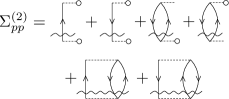
Figure 2: Second-order thermal Dyson self-energy diagrams in the zero-temperature reference [Eq. (36)], which are obtained by deleting an edge in each of the internal energy diagrams in Fig. 1. See also the caption of Fig. 1 as well as Refs. Hirata, 2021a; Hirata et al., 2017.

With these definitions, the thermodynamic relation of Eq. (31) is satisfied by construction. The next one,

$$-\frac{\partial\Omega^{\text{QP(2)}}}{\partial\mu^{\text{QP(2)}}} = \bar{N},$$ (37)

is also obeyed, which can be confirmed by explicit evaluation of the derivative.

$$-\frac{\partial\Omega^{\text{QP(2)}}}{\partial\mu^{\text{QP(2)}}} = -\sum_{p}\frac{\partial\epsilon_{p}^{\text{HF}}}{\partial\mu^{\text{QP(2)}}}f_{p}^{-}+\sum_{p}f_{p}^{-}$$ (38)

$$-\sum_{p}\left(\epsilon_{p}^{\text{HF}}-\mu^{\text{QP(2)}}\right)\frac{\partial f_{p}^{-}}{\partial\mu^{\text{QP(2)}}}$$

$$+\sum_{p,q}\langle pq||pq\rangle\frac{\partial f_{p}^{-}}{\partial\mu^{\text{QP(2)}}}f_{q}^{-}$$

$$-\frac{1}{\beta}\sum_{p}\frac{\partial f_{p}^{-}}{\partial\mu^{\text{QP(2)}}}\ln f_{p}^{-}-\frac{1}{\beta}\sum_{p}\frac{\partial f_{p}^{-}}{\partial\mu^{\text{QP(2)}}}$$

$$-\frac{1}{\beta}\sum_{p}\frac{\partial f_{p}^{+}}{\partial\mu^{\text{QP(2)}}}\ln f_{p}^{+}-\frac{1}{\beta}\sum_{p}\frac{\partial f_{p}^{+}}{\partial\mu^{\text{QP(2)}}}-\frac{\partial\langle E^{(2)}\rangle}{\partial\mu^{\text{QP(2)}}}$$

$$= \sum_{p}f_{p}^{-}-\sum_{p}\left(\epsilon_{p}^{\text{HF}}-\mu^{\text{QP(2)}}\right)\frac{\partial f_{p}^{-}}{\partial\mu^{\text{QP(2)}}}$$

$$-\frac{1}{\beta}\sum_{p}\frac{\partial f_{p}^{-}}{\partial\mu^{\text{QP(2)}}}\ln\frac{f_{p}^{-}}{f_{p}^{+}}-\frac{\partial\langle E^{(2)}\rangle}{\partial\mu^{\text{QP(2)}}}$$

$$= \sum_{p}f_{p}^{-}+\sum_{p}\Sigma_{pp}^{(2)}\frac{\partial f_{p}^{-}}{\partial\mu^{\text{QP(2)}}}-\frac{\partial\langle E^{(2)}\rangle}{\partial\mu^{\text{QP(2)}}}$$

$$= \sum_{p}f_{p}^{-}=\bar{N},$$

where we used

$$\frac{\partial f_{p}^{+}}{\partial\mu^{\text{QP(2)}}} = -\frac{\partial f_{p}^{-}}{\partial\mu^{\text{QP(2)}}},$$ (39)

$$\ln\frac{f_{p}^{-}}{f_{p}^{+}} = -\beta\left(\epsilon_{p}^{\text{QP(2)}}-\mu^{\text{QP(2)}}\right),$$ (40)

but not the explicit derivative $\partial f_{p}^{-}/\partial\mu^{\text{QP(2)}}$, which is a solution of a system of linear equations and cannot be written in a closed form.Gu and Hirata (2024) This justifies the condition for $\mu^{\text{QP(2)}}$ [Eq. (32)].

In the penultimate equality of Eq. (38), we also used

$$\sum_{p}\Sigma_{pp}^{(2)}\frac{\partial f_{p}^{-}}{\partial\mu^{\text{QP(2)}}}=\frac{\partial\langle E^{(2)}\rangle}{\partial\mu^{\text{QP(2)}}},$$ (41)

which can be verified by using Eqs. (LABEL:E2) and (36). In fact, the form of $\Sigma_{pp}^{(2)}$ is determined such that the above equation is satisfied in the first place. Generally,

$$\Sigma_{pp}^{(n)}\equiv\frac{\partial\langle E^{(n)}\rangle}{\partial f_{p}^{-}},$$ (42)

which ensures that Eq. (41) and all similar relations hold.

Equation (42) is a finite-temperature generalizationMatsubara (1955); Luttinger and Ward (1960) of the $n$th-order self-energy of Feynman–Dyson MBGF in the diagonal, frequency-independent approximation.Hirata et al. (2017, 2015) Owing to this diagonal construction, the second- and higher-order thermal quasi-particle theories do not involve rotation of orbitals, unlike thermal HF theoryMermin (1963); Gu and Hirata (2024) or Feynman–Dyson MBGF without the diagonal approximation,Hirata et al. (2017) which define the HF or Dyson orbitalsOrtiz (2020) as those that bring the Fock or self-energy matrix into a diagonal form. Despite the absence of orbital rotation, $\Omega^{\text{QP(2)}}$ is still minimized by varying $f_{p}^{-}$ (see below).

Diagrammatically, the differentiation with respect to $f_{p}^{-}$ corresponds to opening a closed, internal-energy diagram by deleting an edge (whose mathematical interpretation is $f_{p}^{\pm}$).Hirata et al. (2017) A physical meaning of thermal self-energies or thermal quasi-particle energies, which are temperature dependent, is discussed in Sec. III.2.

The following thermodynamic relation,

$$-\frac{\partial\Omega^{\text{QP(2)}}}{\partial T} = S^{\text{QP(2)}},$$ (43)

is also obeyed. This too can be confirmed by explicit differentiation.

$$-\frac{\partial\Omega^{\text{QP(2)}}}{\partial T} = k_{\text{B}}\beta^{2}\frac{\partial\Omega^{\text{QP(2)}}}{\partial\beta}$$ (44)

$$= k_{\text{B}}\beta^{2}\sum_{p}\frac{\partial\epsilon_{p}^{\text{HF}}}{\partial\beta}f_{p}^{-}$$

$$+k_{\text{B}}\beta^{2}\sum_{p}\left(\epsilon_{p}^{\text{HF}}-\mu^{\text{QP(2)}}\right)\frac{\partial f_{p}^{-}}{\partial\beta}$$

$$-k_{\text{B}}\beta^{2}\sum_{p,q}\langle pq||pq\rangle\frac{\partial f_{p}^{-}}{\partial\beta}f_{q}^{-}$$

$$-k_{\text{B}}\left(f_{p}^{-}\ln f_{p}^{-}+f_{p}^{+}\ln f_{p}^{+}\right)$$

$$+k_{\text{B}}\beta\sum_{p}\frac{\partial f_{p}^{-}}{\partial\beta}\ln\frac{f_{p}^{-}}{f_{p}^{+}}$$

$$+k_{\text{B}}\beta^{2}\frac{\partial\langle E^{(2)}\rangle}{\partial\beta}$$

$$= -k_{\text{B}}\left(f_{p}^{-}\ln f_{p}^{-}+f_{p}^{+}\ln f_{p}^{+}\right)$$

$$-k_{\text{B}}\beta^{2}\sum_{p}\Sigma_{pp}^{(2)}\frac{\partial f_{p}^{-}}{\partial\beta}+k_{\text{B}}\beta^{2}\frac{\partial\langle E^{(2)}\rangle}{\partial\beta}$$

$$= -k_{\text{B}}\left(f_{p}^{-}\ln f_{p}^{-}+f_{p}^{+}\ln f_{p}^{+}\right)=S^{\text{QP(2)}},$$

where we used Eqs. (39), (40), and (42), but not the explicit derivative $\partial f_{p}^{-}/\partial\beta$.Gu and Hirata (2024) This justifies the entropy formula [Eq. (29)].

It can also be shown that thermal QP(2) theory is variational with respect to the diagonal elements of its one-electron density matrix, but not with respect to orbitals.

$$\frac{\partial\Omega^{\text{QP(2)}}}{\partial f_{p}^{-}} = \left(\epsilon_{p}^{\text{HF}}-\mu^{\text{QP(2)}}\right)+\sum_{q}\frac{\partial\epsilon_{q}^{\text{HF}}}{\partial f_{p}^{-}}f_{q}^{-}-\sum_{q}\langle pq||pq\rangle f_{q}^{-}$$

$$+\frac{1}{\beta}\ln\frac{f_{p}^{-}}{f_{p}^{+}}+\frac{\partial\langle E^{(2)}\rangle}{\partial f_{p}^{-}}$$

$$= \left(\epsilon_{p}^{\text{HF}}-\mu^{\text{QP(2)}}\right)-\left(\epsilon_{p}^{\text{QP(2)}}-\mu^{\text{QP(2)}}\right)+\Sigma_{pp}^{(2)}=0,$$

where Eq. (42) was used. This proves that the $f_{p}^{-}$ functions that minimize $\Omega^{\text{QP(2)}}$ take the forms of the Fermi–Dirac distribution functions, justifying Eqs. (33)–(35).

Insofar as Eq. (42) is satisfied (and thus all thermodynamic relations are obeyed and the variationality is ensured), there is considerable latitude in selecting the functional form of an approximate internal energy. For instance, the most notable departure of $U^{\text{QP(2)}}$ in Eq. (LABEL:QP:U) from the lengthy, but full $U^{(2)}$ of Eq. (74) of Ref. Hirata and Jha, 2020 is the absence of the so-called anomalous-diagram terms,Kohn and Luttinger (1960); Luttinger and Ward (1960) which sum over the set of indexes whose fictitious denominator is zero.Hirata and Jha (2020); Hirata (2021a) They are purposefully neglected in our ansatz because they are found to cause a severe Kohn–Luttinger nonconvergence problemKohn and Luttinger (1960); Luttinger and Ward (1960); Hirata (2021b, 2022) in $\Sigma_{pp}^{(2)}$, and are undesirable. This issue will be expounded in Appendix A.

When the reference wave function is supplied by a finite-temperature theory, its $\epsilon_{p}^{(0)}$ depends on temperature and the formulas for the thermal self-energies need to be adjusted accordingly. In the thermal HF reference, the second-order thermal self-energy $\Sigma_{pp}^{(2)}$ is found to contain third-order energy-independent terms.Purvis and Öhrn (1975); Schirmer and Angonoa (1989) Although they seem no more expensive to evaluate than the rest, we will not consider this reference any further in this initial study.

Not only is finite-temperature MBPT plagued by the Kohn–Luttinger nonconvergence,Hirata (2021b, 2022) but the Feynman–Dyson perturbation series of zero-temperature MBGF is also shown to display even severer divergence for most low- and high-lying states.Hirata et al. (2024) Potential impact of the latter divergence on thermal quasi-particle theories will be contemplated in Appendix B.

III Numerical results

III.1 Thermodynamic functions

Table 1: Grand potential $\Omega$ (in $E_{\text{h}}$) of an ideal gas of the identical hydrogen fluoride molecules (0.9168 Å) in the STO-3G basis set as a function of temperature ($T$).

$T$ / K	HF	MBPT(2)	QP(2)	FCI
$10^{4}$	$-99.50758$	$-99.94001$	$-99.94179$	$-99.94377$
$10^{5}$	$-101.02137$	$-103.48646$	$-101.30202$	$-102.10659$
$10^{6}$	$-150.56294$	$-151.43748$	$-150.60284$	$-151.24440$
$10^{7}$	$-729.93806$	$-730.10421$	$-729.94666$	$-730.09519$
$10^{8}$	$-6846.98049$	$-6847.00261$	$-6846.98165$	$-6847.00247$

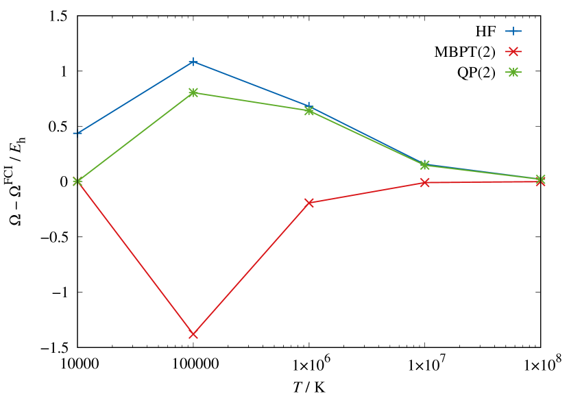
Figure 3: The deviation from thermal FCI theory in grand potential $\Omega$ of an ideal gas of the identical hydrogen fluoride molecules (0.9168 Å) in the STO-3G basis set as a function of temperature ($T$). The “HF” stands for thermal HF theory, “MBPT(2)” denotes second-order finite-temperature many-body perturbation theory with the zero-temperature HF reference, “QP(2)” designates second-order thermal quasi-particle theory with the zero-temperature HF reference.

Table 2: Same as Table 1 but for internal energy $U$ (in $E_{\text{h}}$).

$T$ / K	HF	MBPT(2)	QP(2)	FCI
$0$	$-98.57076$	$-98.58809$	$-98.58809$	$-98.59658$
$10^{4}$	$-98.57076$	$-98.58809$	$-98.58809$	$-98.59658$
$10^{5}$	$-97.94385$	$-97.86604$	$-97.97596$	$-98.04938$
$10^{6}$	$-96.79410$	$-96.99284$	$-96.80270$	$-96.94534$
$10^{7}$	$-92.02773$	$-92.05724$	$-92.02910$	$-92.05557$
$10^{8}$	$-88.48266$	$-88.48744$	$-88.48288$	$-88.48740$

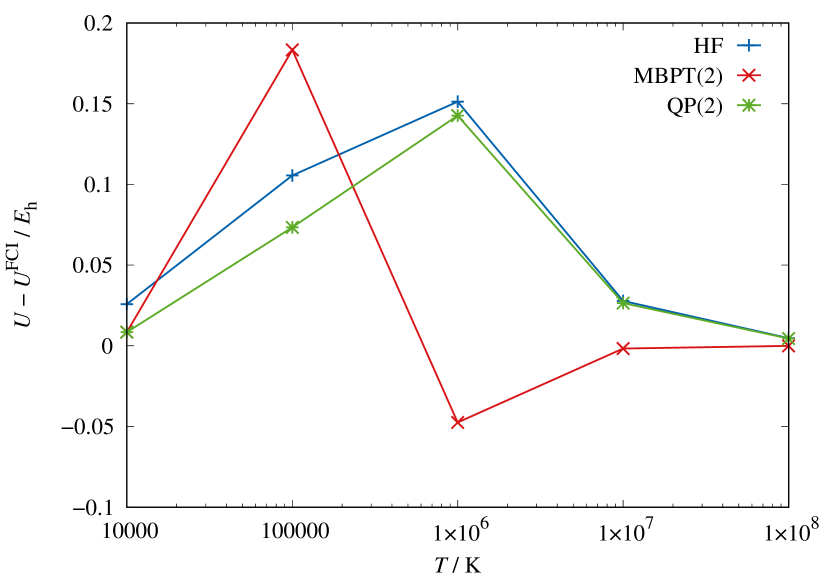
Figure 4: Same as Fig. 3 but for internal energy $U$.

Table 3: Same as Table 1 but for chemical potential $\mu$ (in $E_{\text{h}}$).

$T$ / K	HF	MBPT(2)	QP(2)	FCI
$10^{4}$	$0.09368$	$0.13519$	$0.13537$	$0.13472$
$10^{5}$	$0.20722$	$0.42903$	$0.23246$	$0.29568$
$10^{6}$	$3.80022$	$3.87744$	$3.80378$	$3.85990$
$10^{7}$	$46.85490$	$46.86975$	$46.85568$	$46.86892$
$10^{8}$	$504.65280$	$504.65478$	$504.65291$	$504.65476$

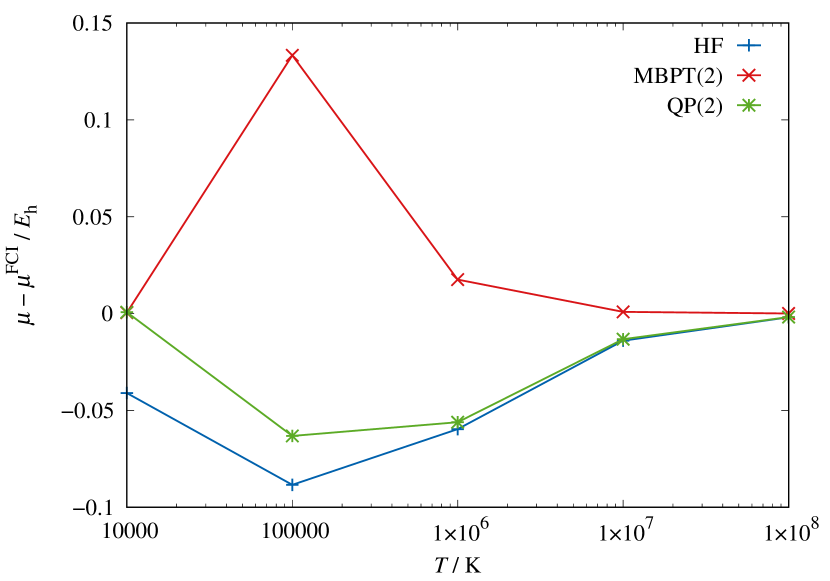
Figure 5: Same as Fig. 3 but for chemical potential $\mu$.

Table 4: Same as Table 1 but for entropy $S$ (in $k_{\text{B}}$).

$T$ / K	HF	MBPT(2)	QP(2)	FCI
$10^{4}$	$0.00000$	$0.00001$	$0.00001$	$0.00011$
$10^{5}$	$3.17451$	$4.20017$	$3.16235$	$3.47472$
$10^{6}$	$4.97871$	$4.94828$	$4.97736$	$4.95769$
$10^{7}$	$5.34800$	$5.34763$	$5.34798$	$5.34766$
$10^{8}$	$5.40597$	$5.40596$	$5.40597$	$5.40596$

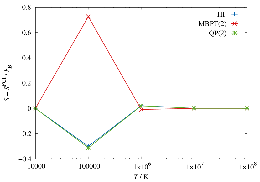
Figure 6: Same as Fig. 3 but for entropy $S$.

Tables 1–4 list the thermodynamic functions—grand potential $\Omega$, internal energy $U$, chemical potential $\mu$, and entropy $S$—of thermal HF [thermal QP(1)],Gu and Hirata (2024) thermal QP(2), fintie-temperature MBPT(2),Hirata and Jha (2020); Hirata (2021a) and thermal full-configuration-interaction (FCI) theoriesKou and Hirata (2014) for an ideal gas of the identical hydrogen fluoride molecules in a wide range of temperature ($T$). Figures 3–6 plot the deviations from thermal FCI benchmarks, the latter being exact within a basis set. The thermal QP(2) and finite-temperature MBPT(2) calculations were based on the zero-temperature HF reference. See Ref. Gu and Hirata, 2024 for the data for the same system from Fermi–Dirac [thermal QP(0)] theory and other thermal mean-field theories, which do not take into account electron correlation.

In all cases, the thermal QP(2) results are close to finite-temperature MBPT(2) ones at low $T$ and are more accurate than thermal HF theory. This is expected because both thermal QP(2) theory and finite-temperature MBPT(2) reduce to zero-temperature MBPT(2) for internal energy, accounting for electron correlation, while thermal and zero-temperature HF theories do not. At higher $T$, thermal QP(2) theory quickly approaches thermal HF theory, where their quasi-independent-particle picture becomes relatively less erroneous. However, at $T=10^{6}$ K and $10^{7}$ K, finite-temperature MBPT(2) is systematically more accurate as it accounts for the effect of electron correlation in $S$ and $\mu$ and it uses more complete second-order corrections (including anomalous-diagram terms) in $\Omega$ and $U$. At the intermediate temperature of $T=10^{5}$ K, thermal QP(2) theory (or even thermal HF theory) outperforms finite-temperature MBPT(2). This may be ascribed to the fact that thermal QP(2) theory includes the effect of electron correlation in the orbital energies, and thus higher-order correlation corrections in a manner similar in spirit to self-consistent Green’s function methods,Luttinger and Ward (1960); Baym and Kadanoff (1961); Baym (1962); Van Neck, Waroquier, and Ryckebusch (1991); Dickhoff (1999); Dickhoff and Barbieri (2004); Dahlen and van Leeuwen (2005); Barbieri (2006); Barbieri and Dickhoff (2009); Phillips and Zgid (2014); Neuhauser, Baer, and Zgid (2017); Tarantino et al. (2017); Kadanoff and Baym (2018); Coveney and Tew (2023) which are said to work for strong correlation. However, this similarity must not be overstated because self-consistent Green’s function methods replace reference orbitals and orbital energies by electron-correlated counterparts, while thermal QP(2) theory uses correlated orbital energies only in the Fermi–Dirac distribution functions and thus reduces identically to MBPT(2) at $T=0$.

Additional numerical data are presented in Supplementary Information,sup which reinforces the foregoing conclusions.

III.2 Thermal quasi-particle energies

Equation (42) can be rewritten as

$$\epsilon_{p}^{\text{QP}}\equiv\frac{\partial U^{\text{QP}}}{\partial f_{p}^{-}},$$ (46)

which encompasses all of the Fermi–Dirac, thermal HF, and thermal QP(2) ansätze.

Hence, the $\epsilon_{p}^{\text{QP}}$ has the literal physical meaning of the increase in the internal energy upon infusion of an infinitesimal fraction of an electron in the $p$th spinorbital. This interpretation can be viewed as a finite-temperature version of Janak’s theoremJanak (1978) in DFT, and may be called thermal Janak’s theorem. It is not unreasonable to consider a fraction of an electron here because the process in question is the thermal average of the same processes involving an infinite number of particles.

While the $\epsilon_{p}^{\text{QP}}$ at $T=0$ is rigorously related to the ionization and electron-attachment energies of a molecule or solid according to Koopmans’ theoremSzabo and Ostlund (1982) or MBGF,Hirata et al. (2017) it cannot be expected to be even close to their thermal averages at $T\gg 0$ because the latter involve different orbitals at different probabilities, even in a strict independent-particle picture.

Therefore, the simplest reasonable approximations to thermal ionization ($I^{\text{QP}}$) and electron-attachment ($A^{\text{QP}}$) energies (signs reversed) based on the $\epsilon_{p}^{\text{QP}}$ may be their weighted averages such as

$$I^{\text{QP}} = \sum_{p}\epsilon_{p}^{\text{QP}}f_{p}^{-}(\bar{N})-\sum_{p}\epsilon_{p}^{\text{QP}}f_{p}^{-}(\bar{N}-1),$$ (47)

$$A^{\text{QP}} = \sum_{p}\epsilon_{p}^{\text{QP}}f_{p}^{-}(\bar{N}+1)-\sum_{p}\epsilon_{p}^{\text{QP}}f_{p}^{-}(\bar{N}),$$ (48)

where $\bar{N}$ is the average number of electrons that ensures electroneutrality and $f_{p}^{-}(N)$ is the Fermi–Dirac distribution function for an arbitrary (integer or noninteger) average number of electrons $N$, i.e.,

$$N=\sum_{p}f_{p}^{-}(N).$$ (49)

It should be understood that only the chemical potential $\mu^{\text{QP}}$ (but not $\epsilon_{p}^{\text{QP}}$) is varied so that this equation is satisfied.

We examine the validity of thermal Janak’s theorem by comparing the above approximations ($I^{\text{QP}}$ and $A^{\text{QP}}$) against $\Delta U^{\text{FCI}}$ defined by

$$\Delta U^{\text{FCI}} \equiv \left\{\begin{array}[]{ll}U^{\text{FCI}}(\bar{N})-U^{\text{FCI}}(\bar{N}-1),&\text{ionization};\\ U^{\text{FCI}}(\bar{N}+1)-U^{\text{FCI}}(\bar{N}),&\text{electron attachment},\end{array}\right.$$ (52)

where $U^{\text{FCI}}(N)$ is the internal energy of thermal FCI theory for an ideal gas of identical molecules, each of which has $N$ electrons on average. It is

$$U^{\text{FCI}}(N) \equiv \frac{\sum_{I}E_{I}e^{-\beta(E_{I}-\mu N_{I})}}{\sum_{I}e^{-\beta(E_{I}-\mu N_{I})}},$$ (54)

where $E_{I}$ is the FCI energy of the $I$th state and the chemical potential $\mu$ is determined by

$$N = \frac{\sum_{I}N_{I}e^{-\beta(E_{I}-\mu N_{I})}}{\sum_{I}e^{-\beta(E_{I}-\mu N_{I})}}.$$ (55)

This is a valid and in fact, exact (within a basis set) treatment of thermodynamics if the particles are not electrically charged. For electrons, however, it describes a physically unrealistic, massively charged plasma, whose energy is not even extensive.Fisher and Ruelle (1966); Dyson and Lenard (1967); Hirata and Ohnishi (2012) Nevertheless, $U^{\text{FCI}}(N)$ and $\Delta U^{\text{FCI}}$ are computationally well defined even for electrons thanks to the ideal-gas assumption (i.e., no interactions between molecules) and will be useful for the following analysis. It may or may not be a reasonable approximation to the thermal average of ionization or electron-attachment energies.

The approximations of Eqs. (47) and (48) imply the corresponding internal-energy functional of the form,

$$U^{\text{QP}}(N)\equiv\sum_{p}\epsilon_{p}^{\text{QP}}f_{p}^{-}(N),$$ (56)

which leads to

$$\Delta U^{\text{QP}} \equiv \left\{\begin{array}[]{ll}I^{\text{QP}},&\text{ionization};\\ A^{\text{QP}},&\text{electron attachment}.\end{array}\right.$$ (59)

The $U^{\text{FCI}}(N)$ and $U^{\text{QP}}(N)$ thus defined are computed for an ideal gas of the identical hydrogen fluoride molecules by thermal FCI, thermal QP(2), and thermal HF theories and are plotted as a function of $N$ in Figs. 7, 8, and 9, respectively. The thermal ionization energies of these three methods are compared with one another and also with the thermal HOMO energies in Table 5. The same data for electron-attachment energies and LUMO are compiled in Table 6.

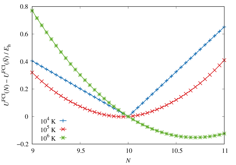
Figure 7: Internal energy of thermal FCI theory $U^{\text{FCI}}$ (in $E_{\text{h}}$) of an ideal gas of the identical hydrogen fluoride molecules (0.9168 Å) in the STO-3G basis set as a function of the average number of electrons $N$ relative to the value at $N=\bar{N}=10$.

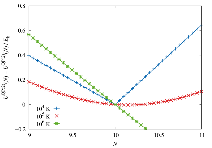
Figure 8: Same as Fig. 7 but for the internal energy of thermal QP(2) theory $U^{\text{QP(2)}}$.

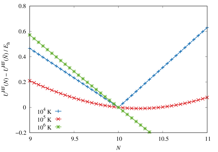
Figure 9: Same as Fig. 7 but for the internal energy of thermal HF theory $U^{\text{HF}}$.

Table 5: Thermal ionization energy (in $E_{\text{h}}$) of an ideal gas of the identical hydrogen fluoride molecules (0.9168 Å) in the STO-3G basis set as a function of temperature ($T$).

	$\epsilon_{p}^{\text{QP}}$		$\Delta U$
$T$ / K	HF	QP(2)	HF	QP(2)	FCI
$0$	$-0.46417$	$-0.39557$	$-0.46417$	$-0.39557$	$-0.40429$
$10^{4}$	$-0.46417$	$-0.39557$	$-0.46589$	$-0.39603$	$-0.40468$
$10^{5}$	$-0.45147$	$-0.41998$	$-0.21004$	$-0.18483$	$-0.32041$
$10^{6}$	$-0.57384$	$-0.57392$	$-0.57181$	$-0.56735$	$-0.77028$
$10^{7}$	$-0.69361$	$-0.69551$	$-3.40146$	$-3.40055$	$-3.65153$
$10^{8}$	$-0.76988$	$-0.77193$	$-4.95141$	$-4.95127$	$-5.34456$

Table 6: Thermal electron-attachment energy (in $E_{\text{h}}$) of an ideal gas of the identical hydrogen fluoride molecules (0.9168 Å) in the STO-3G basis set as a function of temperature ($T$).

	$\epsilon_{p}^{\text{QP}}$		$\Delta U$
$T$ / K	HF	QP(2)	HF	QP(2)	FCI
$0$	$0.62924$	$0.64424$	$0.62924$	$0.64424$	$0.65170$
$10^{4}$	$0.62924$	$0.64424$	$0.62924$	$0.64424$	$0.65170$
$10^{5}$	$0.48080$	$0.50816$	$0.07823$	$0.10621$	$0.40988$
$10^{6}$	$0.28118$	$0.31458$	$-0.55009$	$-0.54444$	$-0.12383$
$10^{7}$	$0.23384$	$0.27782$	$-3.14063$	$-3.13959$	$-2.71365$
$10^{8}$	$0.21118$	$0.26168$	$-4.90424$	$-4.90408$	$-4.48208$

From the tables, we observe that while the HOMO and LUMO energies of thermal quasi-particle theories correctly reduce to the ionization and electron-attachment energies of MBGF in the $T=0$ limit, they clearly have nothing to do with the approximate thermal ionization or electron-attachment energies as defined by $\Delta U^{\text{FCI}}$ at $T\gg 0$, notwithstanding the questionable validity of the latter. However, $\Delta U^{\text{QP}}$ calculated with $\epsilon_{p}^{\text{QP}}$ are in line with the approximate thermal ionization or electron-attachment energies, giving credence to the physical meaning of thermal orbital energies provided by thermal Janak’s theorem.

Thermal QP(2) theory is much closer to thermal FCI theory than thermal HF theory at low temperatures ($T\leq 10^{4}$ K), correctly accounting for electron correlation in thermal ionization and electron-attachment energies. However, at higher $T$, thermal HF and QP(2) theories are essentially the same, suggesting that the effect of electron correlation is surpassed by the lack thereof in the entropy and chemical-potential terms that dominate at such temperatures.

The figures reinforce these observations, but provide the following additional insights: As $T$ is lowered, all $U(N)$ curves begin to display signs of a derivative discontinuity at $N=\bar{N}$, although the strict discontinuity does not occur until $T=0$. Recall that all nonhybrid DFT approximations lack a derivative discontinuity,Perdew and Levy (1983) causing a gross underestimation of band gaps. In both the low- and high-$T$ extremes, $U(N)$ has near-linear dependence on $N$ within each interval between adjacent integers, but at intermediate $T$, each $U(N)$ curve is convex with its minimum occurring away from $N=\bar{N}$.

Let us consider the slope of $U^{\text{QP}}(N)$ at $N=\bar{N}$, which is another macroscopic quantity evaluable with $\epsilon_{p}^{\text{QP}}$.

$$\frac{\partial U^{\text{QP}}}{\partial N} = \frac{\partial\mu^{\text{QP}}}{\partial N}\sum_{p}\frac{\partial f_{p}^{-}}{\partial\mu^{\text{QP}}}\frac{\partial U^{\text{QP}}}{\partial f_{p}^{-}}$$ (60)

$$= \frac{\sum_{p}f_{p}^{-}f_{p}^{+}\epsilon_{p}^{\text{QP}}}{\sum_{p}f_{p}^{-}f_{p}^{+}},$$

where we used Eq. (55) and

$$\frac{\partial f_{p}^{-}}{\partial\mu^{\text{QP}}}=\beta f_{p}^{-}f_{p}^{+}.$$ (61)

This is the increase in the internal energy upon infusion of an infinitesimal fraction of an electron into every molecule in the ideal gas. It is a weighted average of $\epsilon_{p}^{\text{QP}}$ over all spinorbitals. It corresponds to neither the ionization nor electron-attachment process because it is oblivious to the sign of the variation in $N$. However, in the $T=0$ limit, it distinguishes these two processes by exhibiting the derivative discontinuity, i.e.,

$$\lim_{T\to 0}\left(\frac{\partial U^{\text{QP}}}{\partial N}\right)_{N=\bar{N}^{-}} = \epsilon_{\text{HOMO}}^{\text{QP}},$$ (62)

$$\lim_{T\to 0}\left(\frac{\partial U^{\text{QP}}}{\partial N}\right)_{N=\bar{N}^{+}} = \epsilon_{\text{LUMO}}^{\text{QP}}.$$ (63)

Until the $T=0$ limit is strictly reached, however, the $U^{\text{QP}}(N)$ curve is smooth everywhere and the slope approaches the midpoint of the HOMO and LUMO energies.Perdew and Levy (1983) For $T\approx 0$,

$$\left(\frac{\partial U^{\text{QP}}}{\partial N}\right)_{N=\bar{N}} \approx \frac{\epsilon_{\text{HOMO}}^{\text{QP}}+\epsilon_{\text{LUMO}}^{\text{QP}}}{2},$$ (64)

which is also equal to the $T=0$ limit of the $\mu^{\text{QP}}$.Hirata and Jha (2019); Hirata (2021b)

Table 7: $\partial U/\partial N$ (in $E_{\text{h}}$) of an ideal gas of the identical hydrogen fluoride molecules (0.9168 Å) in the STO-3G basis set as a function of temperature ($T$).

$T$ / K	HF	QP(2)	FCI
$0$	$0.08253$	$0.12433$	$0.12371$
$10^{4}$	$0.08189$	$0.12461$	$0.12351$
$10^{5}$	$-0.07423$	$-0.04741$	$0.04959$
$10^{6}$	$-0.56092$	$-0.55587$	$-0.44097$
$10^{7}$	$-3.26523$	$-3.26425$	$-3.17327$
$10^{8}$	$-4.92771$	$-4.92757$	$-4.91206$

Table 7 compares the slope $\partial U/\partial N$ at $N=\bar{N}$ computed analytically by Eq. (60) for thermal HF and QP(2) theories against the slope of thermal FCI theory obtained by numerical differentiation. The three sets of values are in reasonable agreement with one another at all $T$ considered. At low $T$, thermal QP(2) theory is in much better agreement with thermal FCI theory than thermal HF theory. This is because the former takes into account electron correlation. At higher $T$, thermal QP(2) and HF theories are more alike than thermal FCI theory, but they all seem to converge at the same high $T$ limit.

To summarize the results of the foregoing analysis, the orbital energies $\epsilon_{p}^{\text{QP}}$ of thermal quasi-particle theories (including thermal HF theory) cannot be directly related to the ionization or electron-attachment energy from/into the $p$th orbital except at $T=0$. This is simply because an ionization in an ideal gas of molecules at $T\gg 0$ is not a removal of an electron from the $p$th orbital in every molecule; rather, it is a removal of an electron from various orbitals of all molecules at some probabilities (even in a strict independent-particle picture). This is, in turn, equivalent to a removal of some fraction of an electron from various orbitals of an “average” molecule. The $\epsilon_{p}^{\text{QP}}$ at $T>0$ signifies the increase in internal energy upon adding an infinitesimal fraction of an electron in the $p$th spinorbital of this average molecule. This interpretation may be called thermal Janak’s theorem.Janak (1978) This quantity may not directly correspond to any observable, but it is likely combined to approximate macroscopic thermodynamic observables, for which thermal QP(2) theory is expected to be more accurate than thermal HF theory. A further analysis is needed to justify the use of these quasi-particle energies in characterizing, e.g., metal-insulator transitions, however.

IV Conclusions

The thermal quasi-particle theory has been introduced. It is a quasi-independent-particle theory and an electron-correlated extension of the widely used thermal HF theory. It is size-consistent and thus directly applicable to electron-correlated energy bands and thermodynamic functions of semiconductors and insulators at finite temperature.

Its entropy and chemical-potential formulas are of the one-electron type,

$$S\equiv-k_{\text{B}}\sum_{p}\left(f_{p}^{-}\ln f_{p}^{-}+f_{p}^{+}\ln f_{p}^{+}\right),$$

and

$$\bar{N}\equiv\sum_{p}f_{p}^{-},$$

where the thermal population $f_{p}^{-}$ is also unchanged from the Fermi–Dirac distribution function,

$$f_{p}^{-}\equiv\frac{1}{1+e^{\beta(\epsilon_{p}-\mu)}},$$

and $f_{p}^{+}=1-f_{p}^{-}$. The orbital energies $\epsilon_{p}$ now become the ones that include the effect of electron correlation by being defined as the correlated, thermal one-electron energies in the spirit of MBGF,

$$\epsilon_{p}\equiv\frac{\partial U}{\partial f_{p}^{-}},$$

where $U$ is a correlated internal energy, whose mathematical form can be postulated on the basis of finite-temperature MBPT through any chosen order. When the grand potential is defined by

$$\Omega\equiv U-\mu\bar{N}-TS,$$

the theory satisfies all fundamental thermodynamic relations and the $\Omega$ is a variational minimum with respect to $f_{p}^{-}$.

Fermi–Dirac and thermal HF theories can be viewed as the zeroth- and first-order instances, respectively, of the thermal quasi-particle theory hierarchy. It can be viewed as a diagonal, frequency-independent approximation to a finite-temperature extension of the inverse Dyson equation, which at zero temperature is an exact one-particle theory.Hirata et al. (2017) In other words, the $\epsilon_{p}$ thus defined is a finite-temperature extension of the Dyson self-energy in the diagonal, frequency-independent approximation.

It has also been revealed that the thermal self-energy suffers from a severe Kohn–Luttinger nonconvergence problem, making it inappropriate to include anomalous-diagram terms in the definition of approximate $U$ or $\Omega$. This may mean that the thermal quasi-particle theory hierarchy is not convergent at exactness, unfortunately.

Our preliminary implementation and comparison with the thermal FCI benchmarks suggests that thermal QP(2) theory performs distinctly better than thermal HF theory at low $T$ and may even outperform finite-temperature MBPT(2) at intermediate $T$ by including electron-correlation effects in the orbital energies. At higher $T$, the entropy contribution dominates and the differences among various methods become relatively insignificant. The zero-temperature limit of thermal QP(2) theory is MBPT(2) for internal energy and MBGF(2) (in the diagonal, frequency-independent approximation) or $\Delta$MP2 for orbital energies.

The direct physical meaning of $\epsilon_{p}$ is the increase in the internal energy upon infusion of an infinitesimal fraction of an electron in the $p$th spinorbital, i.e., thermal Janak’s theorem.Janak (1978) It does not correspond to the ionization energy or electron-attachment energy of a gas of molecules or a solid at $T>0$. However, it can be used as the key ingredients from which electron-correlated thermodynamic observables can be computed.

Appendix A Kohn–Luttinger nonconvergence

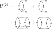
Figure 10: Second-order internal energy diagrams of Eq. (67), which include anomalous (second and fourth) diagrams with no resolvent lines.

According to finite-temperature MBPT,Hirata and Jha (2019, 2020); Hirata (2021a) a more complete expression for the second-order internal energy should include the so-called anomalous-diagram contributions.Kohn and Luttinger (1960) It may read

$$U^{\text{QP}} \equiv \langle E^{(0)}\rangle+\langle E^{(1)}\rangle+U^{(2)}$$ (65)

with

$$U^{(2)} \equiv \langle E^{(2)}\rangle-\beta\langle E^{(1)}E^{(1)}\rangle+\beta\langle E^{(1)}\rangle\langle E^{(1)}\rangle$$ (66)

$$= \langle E^{(2)}\rangle-\beta\langle E^{(1)}E^{(1)}\rangle_{L},$$

where subscript “$L$” means that only diagrammatically linked contributions are to be retained, and the last term (carrying a $\beta$ multiplier) is the anomalous-diagram term. This is still far from the whole second-order internal energy [Eq. (74) of Ref. Hirata and Jha, 2020], but the presence of the last anomalous-diagram term will make clear that this ansatz is unworkable.

The zeroth-order thermal averages in the above expression can be evaluatedHirata and Jha (2020); Hirata (2021a) as

$$U^{(2)} = \sum_{p,q}^{\text{denom.}\neq 0}\frac{F_{qp}F_{pq}}{\epsilon_{p}^{(0)}-\epsilon_{q}^{(0)}}f_{p}^{-}f_{q}^{+}$$ (67)

$$-{\beta}\sum_{p,q}^{\text{denom.}=0}{F_{qp}F_{pq}f_{p}^{-}f_{q}^{+}}$$

$$+\frac{1}{4}\sum_{p,q,r,s}^{\text{denom.}\neq 0}\frac{\langle pq||rs\rangle\langle rs||pq\rangle}{\epsilon_{p}^{(0)}+\epsilon_{q}^{(0)}-\epsilon_{r}^{(0)}-\epsilon_{s}^{(0)}}f_{p}^{-}f_{q}^{-}f_{r}^{+}f_{s}^{+}$$

$$-\frac{\beta}{4}\sum_{p,q,r,s}^{\text{denom.}=0}{\langle pq||rs\rangle\langle rs||pq\rangle}f_{p}^{-}f_{q}^{-}f_{r}^{+}f_{s}^{+},$$

whose diagrammatic representation is given in Fig. 10.

The second and fourth terms (carrying a $\beta$ multiplier but no denominator) are anomalous-diagram terms,Kohn and Luttinger (1960) causing the low-temperature breakdown known as the Kohn–Luttinger nonconvergence.Kohn and Luttinger (1960); Luttinger and Ward (1960); Hirata (2021b, 2022) Take the second term for example. The “denom.=0” restricts the summation to over those combinations of indexes whose fictitious denominator $\epsilon_{p}^{(0)}-\epsilon_{q}^{(0)}$ is zero. One such combination is $p=q$. As $T$ is lowered to zero (i.e., $\beta\to\infty$),Kohn and Luttinger (1960)

$$\lim_{T\to 0}\beta f_{p}^{-}f_{p}^{+}=\delta\left(\mu-\epsilon_{p}^{(0)}\right),$$ (68)

where the right-hand side is Dirac’s delta function, which is divergent when the chemical potential $\mu$ coincides with one of the orbital energies.Kohn and Luttinger (1960) Therefore, a Kohn–Luttinger nonconvergence occurs when $F_{pp}\neq 0$ and at the same time, the reference wave function is degenerate (i.e., the HOMO and LUMO have the same energy as $\mu$). While the divergence of this term can be avoided by adopting a HF reference wherein $F_{pq}=0$,Luttinger and Ward (1960) the fourth term remains divergent for $p=r$ and $q=s$ in a degenerate reference.Hirata (2021b, 2022) It should be recalled that the second-order correction to the ground-state energy is always finite regardless of whether the zeroth-order ground state is degenerateHirschfelder and Certain (1974) or nondegenerate.Shavitt and Bartlett (2009) Hence, $U^{(2)}$ is not convergent at the correct zero-temperature limit, which is always finite.

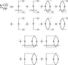
Figure 11: Second-order thermal Dyson self-energy diagrams of Eq. (69), which include anomalous diagrams with no resolvent lines. They are obtained by deleting an edge in each of the internal energy diagrams of Fig. 10.

As per Eq. (42), the corresponding thermal self-energy is obtained by taking the derivative of $U^{(2)}$ with respect to $f_{p}^{-}$, leading to

$$\Sigma_{pp}^{(2)} \equiv \frac{\partial U^{(2)}}{\partial f_{p}^{-}}$$ (69)

$$= \sum_{q}^{\text{denom.}\neq 0}\frac{F_{qp}F_{pq}}{\epsilon_{p}^{(0)}-\epsilon_{q}^{(0)}}f_{q}^{+}-\sum_{q}^{\text{denom.}\neq 0}\frac{F_{pq}F_{qp}}{\epsilon_{q}^{(0)}-\epsilon_{p}^{(0)}}f_{q}^{-}$$

$$+\sum_{q,r}^{\text{denom.}\neq 0}\frac{\langle qp||rp\rangle F_{rq}}{\epsilon_{r}^{(0)}-\epsilon_{q}^{(0)}}f_{r}^{-}f_{q}^{+}$$

$$+\sum_{q,r}^{\text{denom.}\neq 0}\frac{F_{qr}\langle rp||qp\rangle}{\epsilon_{r}^{(0)}-\epsilon_{q}^{(0)}}f_{r}^{-}f_{q}^{+}$$

$$-{\beta}\sum_{q}^{\text{denom.}=0}F_{qp}F_{pq}f_{q}^{+}+{\beta}\sum_{q}^{\text{denom.}=0}F_{pq}F_{qp}f_{q}^{-}$$

$$-{\beta}\sum_{q,r}^{\text{denom.}=0}{\langle qp||rp\rangle F_{rq}f_{r}^{-}f_{q}^{+}}$$

$$-{\beta}\sum_{q,r}^{\text{denom.}=0}{F_{qr}\langle rp||qp\rangle f_{r}^{-}f_{q}^{+}}$$

$$+\frac{1}{2}\sum_{q,r,s}^{\text{denom.}\neq 0}\frac{\langle pq||rs\rangle\langle rs||pq\rangle}{\epsilon_{p}^{(0)}+\epsilon_{q}^{(0)}-\epsilon_{r}^{(0)}-\epsilon_{s}^{(0)}}f_{q}^{-}f_{r}^{+}f_{s}^{+}$$

$$-\frac{1}{2}\sum_{q,r,s}^{\text{denom.}\neq 0}\frac{\langle rs||pq\rangle\langle pq||rs\rangle}{\epsilon_{r}^{(0)}+\epsilon_{s}^{(0)}-\epsilon_{p}^{(0)}-\epsilon_{q}^{(0)}}f_{q}^{+}f_{r}^{-}f_{s}^{-}$$

$$-\frac{\beta}{2}\sum_{q,r,s}^{\text{denom.}=0}{\langle pq||rs\rangle\langle rs||pq\rangle}f_{q}^{-}f_{r}^{+}f_{s}^{+}$$

$$+\frac{\beta}{2}\sum_{q,r,s}^{\text{denom.}=0}{\langle rs||pq\rangle\langle pq||rs\rangle}f_{q}^{+}f_{r}^{-}f_{s}^{-}.$$

The corresponding diagrams are shown in Fig. 11, which are obtained by opening each of the $U^{(2)}$ diagrams in Fig. 10 by deleting an edge. Note the presence of numerous anomalous diagrams.

This formula suffers from a more pervasive kind of the Kohn–Luttinger nonconvergence problem. Take the last term for example. It sums over a set of indexes whose fictitious denominator $\epsilon_{r}^{(0)}+\epsilon_{s}^{(0)}-\epsilon_{p}^{(0)}-\epsilon_{q}^{(0)}$ is zero. It includes the $p=r$ and $q=s$ case, whose summand diverges as $T\to 0$ ($\beta\to\infty$) for any reference—degenerate or nondegenerate—because a $f_{p}^{+}$ factor is no longer there to create a delta function [Eq. (68)] which diverges only when $\mu=\epsilon_{p}^{(0)}$. In other words, a finite-temperature generalization of the self-energy containing anomalous-diagram terms is always divergent as $T\to 0$ and will be uselessly erroneous at low $T$.

This is not surprising because in thermodynamics all states with any number of electrons are summed over in the partition function and they include numerous exactly degenerate zeroth-order states. This is why we purposefully neglected anomalous-diagram terms when defining $U^{\text{QP(2)}}$. Generally, it is inappropriate to include them in the internal energy or grand potential, when their (closed) diagrams will be opened to form some kind of potentials.

This bodes ill for the Luttinger–Ward functionalLuttinger and Ward (1960); Baym and Kadanoff (1961); Baym (1962); Kozik, Ferrero, and Georges (2015); Rossi and Werner (2015); Welden, Rusakov, and Zgid (2016); Gunnarsson et al. (2017); Lin and Lindsey (2018) because opening a diagram of this functional may also result in thermal self-energy and Green’s function diagrams that suffer from the same severe low-temperature breakdown.

Appendix B Feynman–Dyson nonconvergence

We reportedHirata et al. (2024) pervasive divergences of a Feynman–Dyson perturbation expansion of the self-energy in many frequency domains. Therefore, apart from the Kohn–Luttinger-type nonconvergence of the thermal self-energy caused by anomalous-diagram terms, the zero-temperature self-energy will already be divergent or at least excessively erroneous for low- and high-lying states. This is alleviated (or hidden from view) by the frequency-independent approximation inherent in the ansatz of thermal quasi-particle theory, but in a solid, whose self-energy forms continuous energy bands, we can no longer hope to be able to avoid this deep-rooted pathology.Hirata et al. (2024)

In a solid-state implementation of thermal QP(2) theory (which is underway in our laboratory), therefore, we will have to introduce active orbitals (or active energy bands) and evaluate only some portions of $\langle E^{(2)}\rangle$ and $\Sigma_{pp}^{(2)}$ involving them. These active orbitals are the ones whose zeroth-order energies fall within the so-called “central overlapping bracket” where the Feynman–Dyson perturbation expansion is guaranteed to have a nonzero radius of convergence.Hirata et al. (2024) Comparative performance of this method for solids will be presented in the future.

References

- Husimi (1940) K. Husimi, “Some formal properties of the density matrix,” Proc. Phys. Math. Soc. Jpn. 22, 264 (1940).
- Mermin (1963) N. D. Mermin, “Stability of the thermal Hartree–Fock approximation,” Ann. Phys. 21, 99–121 (1963).
- Gu and Hirata (2024) P. Gu and S. Hirata, “Thermal mean-field theories,” Journal Vol., page (the preceding article) (2024).
- Farid, March, and Theophilou (2000) B. Farid, N. H. March, and A. K. Theophilou, “Many-body partition function and thermal Hartree–Fock approximations,” Phys. Rev. E 62, 134–140 (2000).
- Argyres, Kaplan, and Silva (1974) P. N. Argyres, T. A. Kaplan, and N. P. Silva, “Consistency of variational approximations in statistical thermodynamics,” Phys. Rev. A 9, 1716–1719 (1974).
- Szabo and Ostlund (1982) A. Szabo and N. S. Ostlund, Modern Quantum Chemistry (MacMillan, New York, 1982).
- Shavitt and Bartlett (2009) I. Shavitt and R. J. Bartlett, Many-Body Methods in Chemistry and Physics (Cambridge University Press, Cambridge, 2009).
- Hermes and Hirata (2015) M. R. Hermes and S. Hirata, “Finite-temperature coupled-cluster, many-body perturbation, and restricted and unrestricted Hartree–Fock study on one-dimensional solids: Luttinger liquids, Peierls transitions, and spin-and charge-density waves,” J. Chem. Phys. 143, 102818 (2015).
- Pain (2011) J. C. Pain, “Koopmans’ theorem in the statistical Hartree–Fock theory,” J. Phys. B. At. Mol. Opt. 44, 145001 (2011).
- Hirata and Jha (2019) S. Hirata and P. K. Jha, “Converging finite-temperature many-body perturbation theory in the grand canonical ensemble that conserves the average number of electrons,” Annu. Rep. Comput. Chem. 15, 17–37 (2019).
- Hirata and Jha (2020) S. Hirata and P. K. Jha, “Finite-temperature many-body perturbation theory in the grand canonical ensemble,” J. Chem. Phys. 153, 014103 (2020).
- Hirata (2021a) S. Hirata, “Finite-temperature many-body perturbation theory for electrons: Algebraic recursive definitions, second-quantized derivation, linked-diagram theorem, general-order algorithms, and grand canonical and canonical ensembles,” J. Chem. Phys. 155, 094106 (2021a).
- Matsubara (1955) T. Matsubara, “A new approach to quantum-statistical mechanics,” Prog. Theor. Phys. 14, 351–378 (1955).
- Luttinger and Ward (1960) J. M. Luttinger and J. C. Ward, “Ground-state energy of a many-fermion system. II,” Phys. Rev. 118, 1417–1427 (1960).
- March, Young, and Sampanthar (1967) N. H. March, W. H. Young, and S. Sampanthar, The Many-Body Problem in Quantum Mechanics (Cambridge University Press, Cambridge, 1967).
- Kadanoff and Baym (2018) L. P. Kadanoff and G. Baym, Quantum Statistical Mechanics (CRC Press, Boca Raton, 2018).
- Linderberg and Öhrn (1973) J. Linderberg and Y. Öhrn, Propagators in Quantum Chemistry (Academic Press, London, 1973).
- Paldus and Čížek (1975) J. Paldus and J. Čížek, “Time-independent diagrammatic approach to perturbationtheory of fermion systems,” Adv. Quantum Chem. 9, 105–197 (1975).
- Cederbaum and Domcke (1977) L. S. Cederbaum and W. Domcke, “Theoretical aspects of ionization potentials and photoelectron spectroscopy: A Green’s function approach,” Adv. Chem. Phys. 36, 205–344 (1977).
- Simons (1977) J. Simons, “Theoretical studies of negative molecular-ions,” Annu. Rev. Phys. Chem. 28, 15–45 (1977).
- Öhrn and Born (1981) Y. Öhrn and G. Born, “Molecular electron propagator theory and calculations,” Adv. Quantum Chem. 13, 1–88 (1981).
- Jørgensen and Simons (1981) P. Jørgensen and J. Simons, Second Quantization-Based Methods in Quantum Chemistry (Academic Press, New York, 1981).
- Oddershede (1987) J. Oddershede, “Propagator methods,” Adv. Chem. Phys. 69, 201–239 (1987).
- Aryasetiawan and Gunnarsson (1998) F. Aryasetiawan and O. Gunnarsson, “The method,” Rep. Prog. Phys. 61, 237–312 (1998).
- Ortiz (1999) J. V. Ortiz, “Toward an exact one-electron picture of chemical bonding,” Adv. Quantum Chem. 35, 33–52 (1999).
- Onida, Reining, and Rubio (2002) G. Onida, L. Reining, and A. Rubio, “Electronic excitations: density-functional versus many-body Green’s-function approaches,” Rev. Mod. Phys. 74, 601–659 (2002).
- Ortiz (2013) J. V. Ortiz, “Electron propagator theory: an approach to prediction and interpretation in quantum chemistry,” WIREs Comput. Mol. Sci. 3, 123–142 (2013).
- Hirata et al. (2017) S. Hirata, A. E. Doran, P. J. Knowles, and J. V. Ortiz, “One-particle many-body Green’s function theory: Algebraic recursive definitions, linked-diagram theorem, irreducible-diagram theorem, and general-order algorithms,” J. Chem. Phys. 147, 044108 (2017).
- Hirata et al. (2024) S. Hirata, I. Grabowski, J. V. Ortiz, and R. J. Bartlett, “Nonconvergence of the Feynman-Dyson diagrammatic perturbation expansion of propagators,” Phys. Rev. A 109, 052220 (2024).
- Hirata (2011) S. Hirata, “Thermodynamic limit and size-consistent design,” Theor. Chem. Acc. 129, 727–746 (2011).
- Janak (1978) J. F. Janak, “Proof that in density-functional theory,” Phys. Rev. B 18, 7165–7168 (1978).
- Hirschfelder and Certain (1974) J. O. Hirschfelder and P. R. Certain, “Degenerate RS perturbation-theory,” J. Chem. Phys. 60, 1118–1137 (1974).
- Bartlett (1981) R. J. Bartlett, “Many-body perturbation theory and coupled cluster theory for electron correlation in molecules,” Annu. Rev. Phys. Chem. 32, 359–401 (1981).
- Hirata et al. (2015) S. Hirata, M. R. Hermes, J. Simons, and J. V. Ortiz, “General-order many-body Green’s function method,” J. Chem. Theory Comput. 11, 1595–1606 (2015).
- Purvis and Öhrn (1975) G. D. Purvis and Y. Öhrn, “Comment on a theory of electron affinities,” Chem. Phys. Lett. 33, 396–398 (1975).
- Schirmer and Angonoa (1989) J. Schirmer and G. Angonoa, “On Green’s-function calculations of the static self-energy part, the ground-state energy and expectation values,” J. Chem. Phys. 91, 1754–1761 (1989).
- Ortiz (2020) J. V. Ortiz, “Dyson-orbital concepts for description of electrons in molecules,” J. Chem. Phys. 153, 070902 (2020).
- Kohn and Luttinger (1960) W. Kohn and J. M. Luttinger, “Ground-state energy of a many-fermion system,” Phys. Rev. 118, 41–45 (1960).
- Hirata (2021b) S. Hirata, “Low-temperature breakdown of many-body perturbation theory for thermodynamics,” Phys. Rev. A 103, 012223 (2021b).
- Hirata (2022) S. Hirata, “General solution to the Kohn–Luttinger nonconvergence problem,” Chem. Phys. Lett. 800, 139668 (2022).
- Kou and Hirata (2014) Z. Kou and S. Hirata, “Finite-temperature full configuration interaction,” Theor. Chem. Acc. 133, 1487 (2014).
- Baym and Kadanoff (1961) G. Baym and L. P. Kadanoff, “Conservation laws and correlation functions,” Phys. Rev. 124, 287–299 (1961).
- Baym (1962) G. Baym, “Self-consistent approximations in many-body systems,” Phys. Rev. 127, 1391–1401 (1962).
- Van Neck, Waroquier, and Ryckebusch (1991) D. Van Neck, M. Waroquier, and J. Ryckebusch, “Self-consistent solution of the second-order Dyson equation for single-particle propagators, with application to the spectral functions of 48Ca,” Nucl. Phys. A 530, 347–369 (1991).
- Dickhoff (1999) W. H. Dickhoff, “The nucleon propagator in the nuclear medium,” in Nuclear Methods and the Nuclear Equation of State, International Review of Nuclear Physics, Vol. 8, edited by M. Baldo (World Scientific, Singapore, 1999) Chap. 7, pp. 326–380.
- Dickhoff and Barbieri (2004) W. H. Dickhoff and C. Barbieri, “Self-consistent Green’s function method for nuclei and nuclear matter,” Prog. Part. Nucl. Phys. 52, 377–496 (2004).
- Dahlen and van Leeuwen (2005) N. E. Dahlen and R. van Leeuwen, “Self-consistent solution of the Dyson equation for atoms and molecules within a conserving approximation,” J. Chem. Phys. 122, 164102 (2005).
- Barbieri (2006) C. Barbieri, “Single particle spectra based on modem effective interactions,” Phys. Lett. B 643, 268–272 (2006).
- Barbieri and Dickhoff (2009) C. Barbieri and W. H. Dickhoff, “Spectroscopic factors in 16O and nucleon asymmetry,” Int. J. Mod. Phys. A 24, 2060–2068 (2009).
- Phillips and Zgid (2014) J. J. Phillips and D. Zgid, “Communication: The description of strong correlation within self-consistent Green’s function second-order perturbation theory,” J. Chem. Phys. 140, 241101 (2014).
- Neuhauser, Baer, and Zgid (2017) D. Neuhauser, R. Baer, and D. Zgid, “Stochastic self-consistent second-order Green’s function method for correlation energies of large electronic systems,” J. Chem. Theory Comput. 13, 5396–5403 (2017).
- Tarantino et al. (2017) W. Tarantino, P. Romaniello, J. A. Berger, and L. Reining, “Self-consistent Dyson equation and self-energy functionals: an analysis and illustration on the example of the Hubbard atom,” Phys. Rev. B 96, 045124 (2017).
- Coveney and Tew (2023) C. J. N. Coveney and D. P. Tew, “A regularized second-order correlation method from Green’s function theory,” J. Chem. Theory Comput. 19, 3915–3928 (2023).
- (54) Supplementary information .
- Fisher and Ruelle (1966) M. E. Fisher and D. Ruelle, “Stability of many-particle systems,” J. Math. Phys. 7, 260–270 (1966).
- Dyson and Lenard (1967) F. J. Dyson and A. Lenard, “Stability of matter. I,” J. Math. Phys. 8, 423–434 (1967).
- Hirata and Ohnishi (2012) S. Hirata and Y. Ohnishi, “Thermodynamic limit of the energy density in a crystal,” Phys. Chem. Chem. Phys. 14, 7800–7808 (2012).
- Perdew and Levy (1983) J. P. Perdew and M. Levy, “Physical content of the exact Kohn-Sham orbital energies: Band gaps and derivative discontinuities,” Phys. Rev. Lett. 51, 1884–1887 (1983).
- Kozik, Ferrero, and Georges (2015) E. Kozik, M. Ferrero, and A. Georges, “Nonexistence of the Luttinger-Ward functional and misleading convergence of skeleton diagrammatic series for Hubbard-like models,” Phys. Rev. Lett. 114, 156402 (2015).
- Rossi and Werner (2015) R. Rossi and F. Werner, “Skeleton series and multivaluedness of the self-energy functional in zero space-time dimensions,” J. Phys. A 48, 485202 (2015).
- Welden, Rusakov, and Zgid (2016) A. R. Welden, A. A. Rusakov, and D. Zgid, “Exploring connections between statistical mechanics and Green’s functions for realistic systems: Temperature dependent electronic entropy and internal energy from a self-consistent second-order Green’s function,” J. Chem. Phys. 145, 204106 (2016).
- Gunnarsson et al. (2017) O. Gunnarsson, G. Rohringer, T. Schäfer, G. Sangiovanni, and A. Toschi, “Breakdown of traditional many-body theories for correlated electrons,” Phys. Rev. Lett. 119, 056402 (2017).
- Lin and Lindsey (2018) L. Lin and M. Lindsey, “Variational structure of Luttinger-Ward formalism and bold diagrammatic expansion for Euclidean lattice field theory,” Proc. Natl. Acad. Sci. (USA) 115, 2282–2286 (2018).