Characterization of a Displaced Coaxial Feed for Cascaded Cylindrical Metasurfaces
Abstract
This paper characterizes a realistic feed for cylindrical metasurfaces, allowing it to be included in metasurface design. Specifically, it investigates a coaxial feed which is displaced from the center (off-center) of concentrically-cascaded cylindrical metasurfaces. Formulas are reported to quickly compute the multimodal -matrix (scattering properties) of a displaced feed from that of the central feed. The theory is rigorously derived based on the addition theorem of Hankel functions for all azimuthal modes. Moreover, the resulting multimodal -matrix is combined with the multimodal wave matrix theory used to model cylindrical metasurfaces, allowing devices to be designed that realize arbitrary field transformations from a displaced coaxial feed. A design example is reported, which opens new opportunities in the realization of realistic, high-performance cylindrical-metasurface-based devices.
Index Terms:
Antenna radiation pattern synthesis, coaxial feeds, curved metasurfaces, cylindrical scatterers, impedance sheets, metasurfaces, wave matrixI Introduction
Concentrically-cascaded cylindrical metasurfaces have been demonstrated that can tailor the amplitude and phase [1, 2, 3, 4], and even the polarization [5, 6] of cylindrical waves. As a result, they have been employed in stealth technology, providing functionalities such as camouflage [7], electromagnetic cloaking [8, 9, 10, 11, 12, 13, 14] and illusion [1, 2, 3, 7, 15]. They have also been used to manipulate the wave propagation [16] and cutoff frequency [17, 18] in circular waveguides, and to design a high gain antenna by shaping the radiation patterns [1, 19]. In addition, cylindrical metasurfaces can be used to generate orbital angular momentum (OAM) waves through azimuthal mode conversion [3, 4, 22, 23, 20, 21]. All the aforementioned applications require arbitrary field transformations which convert a known excitation field to the desired or stipulated output field.
Previous approaches to achieve arbitrary field transformations through cascaded cylindrical metasurfaces were mostly based on the Generalized Sheet Transition Condition (GSTC) [24, 25, 26, 27, 28, 29], which suffers greatly from realization limitations such as extremely small layer separations [1, 24, 25] an the need for perfectly conducting baffles between unit cells [1, 20]. In contrast, multimodal wave matrix theory [3, 4] is able to accurately capture the higher-azimuthal-order coupling and lateral wave propagation between the cascaded cylindrical metasurface layers, making it ideal for analyzing and synthesizing such structures. Using the multimodal wave matrix theory, an azimuthal mode converter and an illusion device have been designed [3]. However, in these earlier works, idealized (fictitious) line currents were assumed as the excitation sources. This impractical assumption neglects possible interaction between the source and metasurfaces.
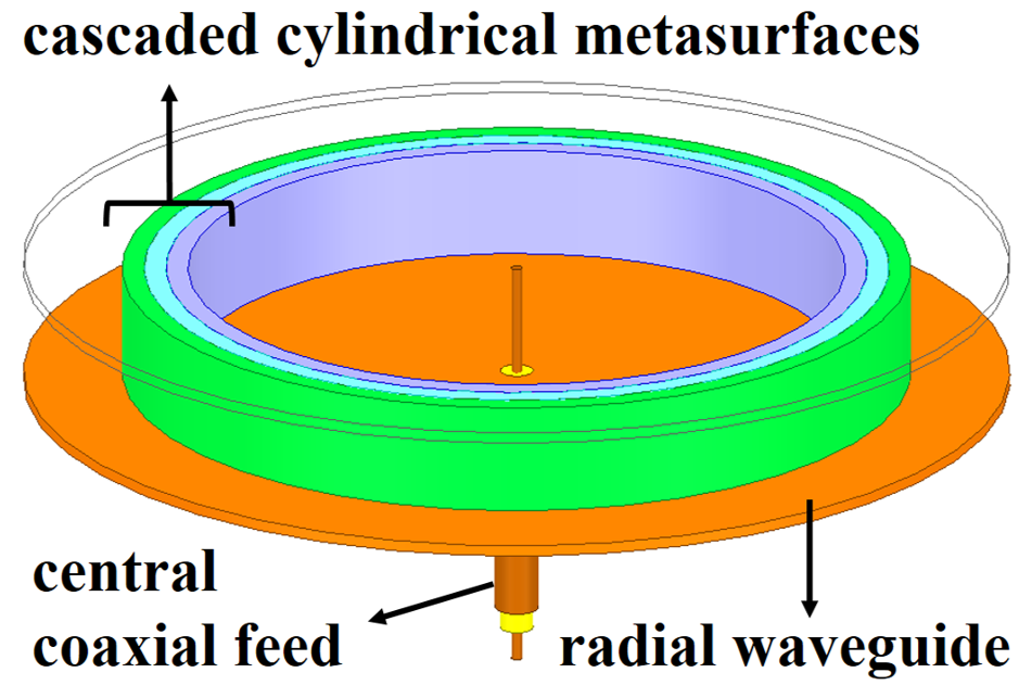
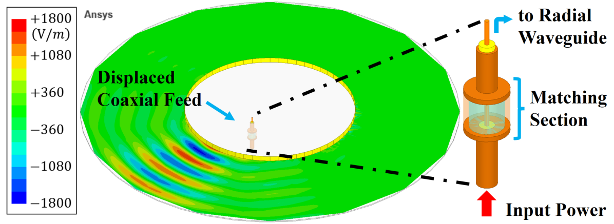
Subsequently, a realistic device, shown in Fig. 1(a), has been developed, which consists of a set of cascaded cylindrical metasurfaces inside a radial waveguide with a realistic, central coaxial feed [22, 23]. The scattering properties of the realistic, central coaxial feed are numerically computed using the mode-matching technique (MMT) [30, 31, 32, 33, 34] and compactly summarized into a multimodal -matrix. This multimodal -matrix is then integrated with the multimodal wave matrix representing the metasurfaces [3, 4]. This allows interactions between the cylindrical metasurfaces and the central coaxial feed to be taken into account. Based on these structures, a coaxially-fed, azimuthal mode converter was realized [22, 23]. These single-input single-output (SISO) devices are able to perform arbitrary field transformations from a central coaxial feed.
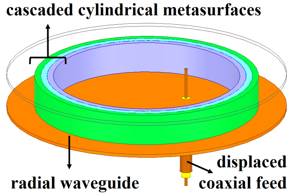
Multiple-input multiple-output (MIMO) devices made from cylindrical metasurfaces can provide for greater functionalities. MIMO cylindrical metasurfaces can be designed to interact with feeds at different locations and produce different output fields. In other words, these MIMO devices incorporate multiple feeds, while only a single, centrally-located coaxial feed for cylindrical metasurfaces was investigated in [22, 23]. Therefore, as a first step toward designing MIMO devices, a realistic coaxial feed displaced from the center of a cylindrical metasurface, illustrated in Fig. 1(b), must be modelled. In [19], the scattering characteristics of a displaced coaxial feed were computed. A beam-shaping shell, consisting of five azimuthally-symmetric cylindrical metasurfaces, was presented, demonstrating the manipulation of electromagnetic fields from a displaced coaxial feed.
In this paper, the theory behind [19] is detailed. To model a displaced coaxial feed, our aim is to derive its multimodal -matrix since this mathematical form is compatible with the multimodal wave matrix theory used to model concentric metasurfaces [3, 4]. Previously, MMT was adopted in order to accurately model the central coaxial feed [22]. However, this method becomes computationally expensive when the feed is off-center. Herein, we present a more elegant and efficient way to characterize the scattering properties of a displaced coaxial feed. First, the multimodal -matrices of the central feed and a displaced feed are defined. Next, the addition theorems of Hankel functions, including all higher-order azimuthal modes [35, 36], are then employed to relate these two matrices. We have shown that the multimodal -matrix of the displaced feed can be derived directly from the known matrix of the central feed in [22, 23]. They are related through simple matrix multiplication. With this result, cascaded cylindrical metasurfaces can be designed to generate any stipulated output field with flexibility over the feed placement. To verify the proposed theory, a beam shaping shell fed by a displaced coaxial feed is presented in this paper. The reflection coefficient of the device is reduced by introducing a quarter-wave impedance transformer to the coaxial feed [37, 38]. This example has two significant implications. First, it showcases that arbitrary field transformations from a displaced coaxial feed can be accomplished. More importantly, it creates a path toward the realization of practical cylindrical-metasurface-based MIMO devices.
II The Proposed Theory
The analysis and synthesis of cylindrical metasurface-based devices excited by a displaced coaxial feed are presented in this section. Derivations of the associated multimodal S-matrices and consequent field representations are given. The characterization of the displaced coaxial feed is discussed in detail.
II-A Proposed Structure and Definitions
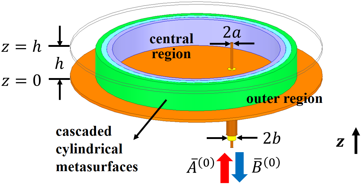
The device considered is illustrated in Fig. 2(a) and details of its layout are given in Fig. 2(b). A set of concentrically-cascaded cylindrical metasurfaces, whose center is set to be the global origin, is inserted within an air-filled parallel-plate radial waveguide. For simplicity, the height of the radial waveguide, , is subject to the following limitation:
| (1) |
where is the angular frequency under the operating frequency, and and are the free-space permittivity and permeability, respectively. This limitation (1) ensures that all the propagating fields in the radial waveguide must be modes and invariant in [22]. Consequently, the electromagnetic problem becomes two-dimentional (2-D) [3]. The device is excited by a realistic coaxial feed which is located off-center at . We assume in the same manner as in [22] that the inner conductor of the feed touches the upper plate of the radial waveguide. To guarantee that only the mode propagates in the coaxial cable, its inner and outer conductor radii , , as well as the filling dielectric permittivity , must satisfy [37]:
| (2) |
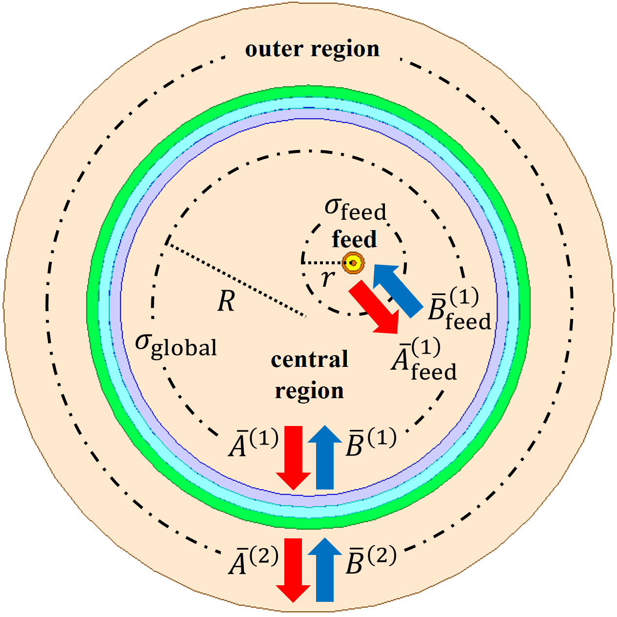
In order to characterize the junction between the coaxial feed and the radial waveguide, a multimodal -matrix can be defined. To this end, the electric field along the cylindrical surface indicated in Fig. 2(b), which is centered about the feed location , is investigated first. The radius of is chosen such that evanescent waves generated from the junction discontinuity have decayed significantly. Under the time convention, the electric field along can be written in terms of propagating cylindrical waves (Hankel functions) centered with respect to :
| (3) |
where is the wave number in the free-space, is the azimuthal angle with respect to , and is a sufficiently large number that ensures the series (3) converges. The first and second series in (3) represent the outgoing and incoming fields, respectively, and are their corresponding wave amplitudes [3].
A multimodal wave matrix can be defined based on vectors representing the complex amplitudes of the azimuthal modes of (3) [3]. However, a multimodal -matrix is defined based on power waves [3, 22]; it requires the normalization of the azimuthal modes [37, 39]. Specifically, we can write the following power waves:
| (4) | ||||
| (5) |
where the vectors ()
| (6) | ||||
| (7) |
contain the wave amplitude of each azimuthal mode. The diagonal matrices and consist of Hankel functions:
| (8) | ||||
| (9) |
and the diagonal matrices and are formed by the normalization constants [3]:
| (10) | ||||
| (11) |
| (12) | ||||
| (13) |
The normalization constants (12) and (13) of an azimuthal mode are found by examining the powers that pass through a cylindrical reference surface [6]. These constants take into account the fact that wave impedances in cylindrical coordinates depend on both the azimuthal order and the radius . Note that the power waves and are vectors. They are defined on and, hence, are centered with respect to , as illustrated in Fig. 2(b).
The normalized waves in the coaxial cable that are incident on and reflected from the junction are denoted by and , respectively (see Fig. 2(b)). They are vectors since only the mode is allowed. Normalization of these two vectors is discussed in [22, 37]. For convenience, the reference surface of the power waves and is defined at the lower plate of the coaxial waveguide, i.e. at the plane indicated in Fig. 2(a) [22]. The multimodal -matrix of the coaxial-waveguide junction can then be defined as,
| (14) |
Consequently, these power waves (14) are centered with respect to the coaxial feed. Therefore, this definition (14) is exactly the multimodal -matrix of the central feed derived in [22] through MMT.
Similarly, we can define a multimodal -matrix of the displaced feed,
| (15) |
where and are both vectors defined on the cylindrical surface shown in Fig. 2(b). The radius of this cylindrical surface is chosen such that fully encloses , namely, . The power waves and are centered with respect to the global origin. These waves are the natural bases of the cylindrical metasurfaces, so they greatly simplify any further analysis.
Analogous to (4) and (5), we write:
| (16) | ||||
| (17) |
in which the diagonal matrices and are similarly defined as in (8)-(13), with the argument replaced with . The vectors are composed of wave amplitudes obtained by expanding the electric field along :
| (18) |
| (19) | ||||
| (20) |
where is the azimuthal angle measured from the global origin. Furthermore, the vectors and are defined in the outer region of Fig. 2(b). They are related to and through the multimodal -matrix of the cascaded cylindrical metasurfaces:
| (21) |
For a given cascaded cylindrical metasurface, its multimodal -matrix can be derived based on the multimodal wave matrix theory detailed in [3].
II-B Analysis and Synthesis
A central aim of this paper is to derive the multimodal -matrix of the displaced feed (15) directly from that of the central feed (14) rather than from the complicated MMT. For this purpose, we employ the addition theorem for Hankel functions of all azimuthal orders:
| (22) |
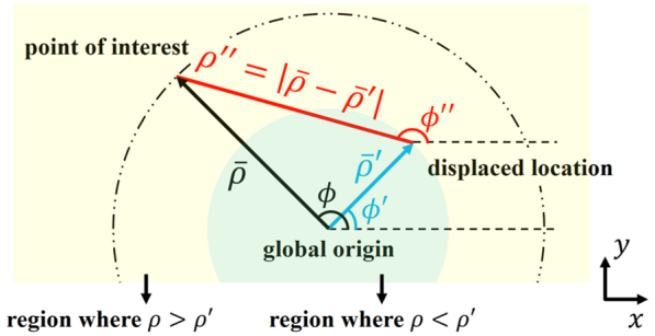
| (23) |
where the geometric parameters are illustrated in Fig. 3(a). The proof of (22) and (23) can be performed by utilizing raising or lowering operators [35], or by matching the large argument approximations of the Hankel and Bessel functions [36]. The first proof is outlined in the Appendix of this paper. In essence, these addition theorems relate cylindrical waves centered with respect to to those centered with respect to the global origin. Therefore, they can help us find the relation between the multimodal -matrices (14) and (15).
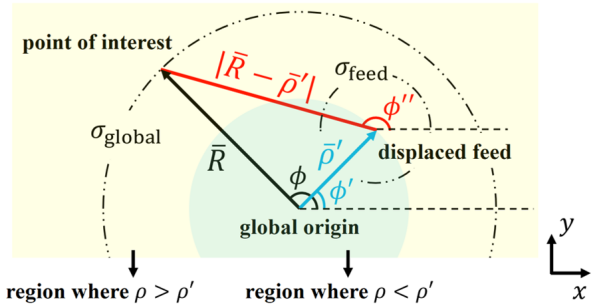
To apply these addition theorems to our system, the outgoing propagating electric field, , along the large cylindrical surface is studied. In this case, , as shown in Fig. 3(b). The field can be expressed in terms of a set of outgoing cylindrical waves centered with respect to the displaced feed ,
| (24) |
Based on our choice of the cylindrical surfaces and , is always greater than . Consequently, the first part of (22) can be applied to (24) to yield:
| (25) |
Notice that the in (25) are exactly the outgoing cylindrical waves centered with respect to the global origin and are evaluated at . Therefore, the term inside the bracket is actually the corresponding wave amplitudes if we expand in terms of these cylindrical waves, as in (18):
| (26) |
| (27) |
This relationship between the wave amplitudes (27) can be rewritten in matrix form using the definitions (6) and (19),
| (28) |
where information on the feed displacement is embedded in the entries of the matrix . Each entry of can be determined by the following equation:
| (29) |
The first index in the square bracket indicates the row number of the entry, and the second index indicates the column number. Note that in (6) and (19), the entries are arranged in a descending azimuthal order (the first entry being the mode and the last being the mode). The indices in (29) are chosen so that they comply with this descending order.
A similar approach can be employed to the incoming propagating electric field, , along . It can be shown that its wave amplitudes are related in the same manner as (28):
| (30) |
It is important to examine how (28)-(30) change when there is no displacement, i.e. when . If there is no displacement, both expansions (3) and (18) should yield the same wave amplitudes. When its argument is zero, the Bessel function of the first kind only has a nonvanishing value when . In fact, this nonvanishing value is unity. Hence, when , (29) reduces to:
| (31) |
which implies that becomes an identity matrix. In other words, and , as expected.
In order to relate the multimodal -matrices (14) and (15), the relationships between power waves rather than those between wave amplitudes are required. By combining (4), (16), and (28), can be neatly expressed in terms of :
| (32) |
Similarly, we have for and ,
| (33) |
Based on the definitions (32) and (33), the dimensions of the matrices and are both .
Now that the relationships between power waves have been found, the multimodal -matrix of a displaced feed can also be derived. By applying (32), (33) and rewriting (15), we obtain:
| (34) |
where , , and denote the identity matrix, zero matrix, and zero matrix, respectively. After rearranging (34) and comparing the result with the definition (14), the following equation is derived:
| (35) |
or equivalently:
| (36) |
where the inversion of block diagonal matrices [40] is utilized. It is clear from (36) that the multimodal -matrix of a displaced feed (15) can be easily obtained from that of the central feed (14). The cumbersome MMT only needs to be conducted once to calculate (14), and any displacement of the coaxial feed can be taken into account through simple matrix multiplication. Consequently, a major goal of this paper has been achieved.
With the scattering information of the displaced feed, a synthesis or design problem can now be tackled. The interaction between this displaced feed and the cascaded cylindrical metasurfaces can be taken into account by solving (15) and (21) jointly. Consider the setup in Fig. 2 again. In theory, there is no reflection from infinity, so we set which is a zero vector. The power waves in the central region can be expressed in terms of the incident power waves from the coaxial feed, , as:
| (37) |
| (38) |
where denotes an identity matrix. By substituting (37) and (38) into (15), the reflected power wave in the coaxial feed is calculated as,
| (39) |
from which the reflection coefficient of the device can be deduced. Alternatively, (21) yields the power wave in the outer region,
| (40) |
Finally, arbitrary field transformations from this displaced coaxial feed are accomplished by matching this power wave to the desired or stipulated field through an optimization algorithm.
III Validation Examples
An innovative antenna beam-shaping shell is demonstrated in this section. The results not only verify the presented theory, but also demonstrate its effectiveness. Moreover, an impedance matching structure is introduced and incorporated into the device to enhance its practical performance characteristics.
III-A The Antenna Beam-Shaping Shell
A beam-shaping shell is developed that converts the input field originating from a displaced coaxial feed to a narrow radiated beam. Although the functionality of the resulting device is similar to the azimuthally-symmetric case presented in [19], the aim herein is to accomplish the design with azimuthally-varying cylindrical metasurfaces. The additional degrees of freedom introduced by azimuthal variation allows for a design with fewer cylindrical metasurface layers. Furthermore, they also help achieve a narrower beam and/or a lower reflection coefficient.
Our goal in this design example is to synthesize a narrow beam radiated in the direction by tailoring cylindrical electromagnetic waves. This idea was inspired by [41, 42] where dielectric shells with large positive and negative relative permittivities were applied to control the cylindrical waves emitted by a line source. Dielectric materials with large negative relative permittivities are difficult to realize. Therefore, cylindrical metasurfaces consisting of patterned metallic claddings on commercial dielectric substrates are utilized to control the radiated waves. Their use furnishes the important advantage of circumventing the need for dielectric materials with extreme relative permittivities.
As presented in [41, 42], the Dirac delta function describes a radiation pattern with an idealized (infinitely narrow) beam pointing solely in the forward () direction. It can be expressed in terms of azimuthal modes based on Fourier series, where the coefficient associated with each mode is identical:
| (41) |
Therefore, we set our target electric field in the outer region of the cylindrical metasurfaces to be:
| (42) |
where is the corresponding wave amplitude of the cylindrical wave with azimuthal order , and is an arbitrary constant. Note that only Hankel functions of the second kind are present in (42) since it is assumed that there are no incoming cylindrical waves from infinity. The reason for setting the target field to (42) can be understood immediately from its far-field expression. In particular, the large argument approximation of the Hankel functions can be employed in the far-field where , i.e., [43]:
| (43) |
Consequently, (42) becomes,
| (44) |
It is clear that the expansion coefficient associated with each azimuthal mode in (44) is identical, as it is in the Dirac delta function (41). Thus, the desired field in the outer region described by (42) yields an idealized (infinitely narrow) radiated beam. In practice, it is impossible to control an infinite number of azimuthal modes. Hence, (41) and (42) need to be truncated. This results in a narrow radiated beam of finite beamwidth in the forward direction.
The operating frequency of our example beam-shaping shell is set at GHz. The displaced feed is located at where denotes the operating wavelength in free-space. The detailed dimensions of the coaxial cable are mm, mm (see Fig. 2), and the dielectric within the cable is Teflon with , making the characteristic impedance of the coaxial cable . A single layer of cylindrical metasurface, whose radius is , is centered with respect to the global origin and placed within a radial waveguide whose height is mm. The physical dimensions of the coaxial cable, as well as the radial waveguide, satisfy (1) and (2). Therefore, the analysis developed in the previous section is a valid approach to evaluate the performance of the example structure. Furthermore, they are also identical to those adopted in [22]. Hence, the multimodal -matrix of the coaxial-waveguide junction (14) is the same as the one obtained in that work.
In multimodal wave matrix theory, a cylindrical metasurface can be described mathematically by a -dependent admittance profile which relates the induced surface current density to the averaged electric field [3]. For a lossless design, is purely imaginary and can be expressed using the susceptance . The susceptance profile of the cylindrical metasurface in our solver was optimized to have the electric field in the outer region, which is related to the power wave given by (40), come as close to the desired field as possible. The target field was selected to consist of the first 11 terms (from to ) of the infinite series (42). In order to avoid highly-oscillatory susceptance profiles which are difficult to realize, we have enforced a smooth, sinusoidal azimuthal variation of in the multimodal wave matrix theory.
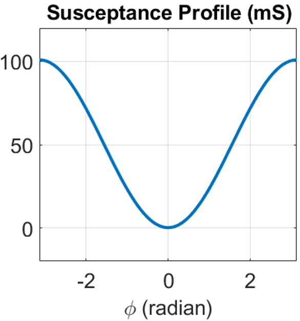
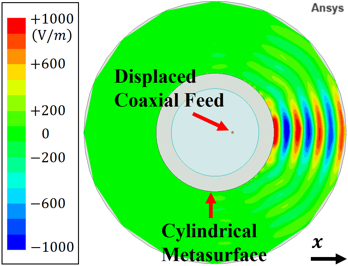
The synthesized results of the beam-shaping shell are shown in Fig. 4. The optimized susceptance profile of the single-layer cylindrical metasurface, illustrated in Fig. 4(a), is discretized into 60 unit cells and implemented as impedance boundary conditions in Ansys HFSS. The smooth azimuthal variation of the susceptance profile indicates another advantage of our formulation: extreme discretization is not required. The simulated performance of the device shown in Fig. 4(b) clearly demonstrates a narrow radiation beam in the direction as specified. Our analysis method predicted a reflection coefficient of at the plane of the coaxial feed in Fig. 2, while the full-wave simulation yielded a value of . These very close values verify its accuracy.
A related characteristic of interest is the 2-D directivity (recall that the field in the radial waveguide is a 2-D one). It is calculated based on the following definition [41, 42]:
| (45) |
If the electric field in the far-field is expressed in terms of azimuthal modes with corresponding coefficients :
| (46) |
then the numerator of (45) can be calculated knowing that,
| (47) |
and, hence, that
| (48) |
Moreover, the integrand of the denominator in (45) can be written as,
| (49) |
After integration, only the terms with remain yielding:
| (50) |
Therefore, the 2-D directivity (45) is readily calculated as:
| (51) |
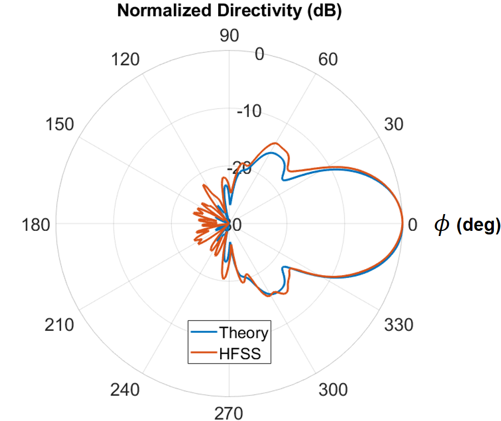
Since only 11 terms in the series (42) representing the radiated field were considered, the highest 2-D directivity that could have been obtained is 11.0 or dB. With the susceptance profile shown in Fig. 4(a), our beam-shaping system produces a 2-D directivity of 10.16 dB, while the corresponding full-wave simulation results in 4(b) attained a value of dB. Additionally, the radiation patterns in the plane calculated from both the theory and the HFSS simulation are plotted and compared in Fig. 5. Close agreement between the two curves is evident. The small lobes in the left portion of the full-wave simulated pattern have been confirmed to be due to the level of discretization of the mesh employed throughout the metasurface and overall structure. The 3-dB beamwidth of the main lobe produced by the designed beam-shaping shell is approximately and the side lobe level is dB. Moreover, the device also offers a very high front-to-back ratio that is greater than dB. This example clearly illustrates the capability of the developed design framework to achieve arbitrary field transformations from a metasurface-based structure excited by a displaced coaxial feed.
III-B The Impedance Matching Structure
Another important figure of merit of practical importance is the input impedance of our structure with a realistic coaxial feed and impedance matching element. Previous researchers have proposed several methods to improve matching to a coaxial feed. A top-loading disk (metallic puck) was inserted into the junction between the coaxial cable and the radial waveguide in [30]. However, this method significantly modifies the feeding structure and, hence, necessitates a recalculation of the MMT-based scattering properties [22, 23, 30, 31, 32, 33, 34]. Another matching technique is to design a quarter-wave impedance transformer within the coaxial cable [37]. Since the impedance transformer is physically separated from the coaxial-waveguide junction, it does not disturb the feeding structure and, therefore, can be applied easily to the device [38].
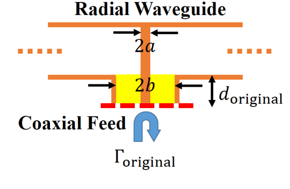
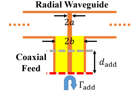
The design evolution of the coaxial quarter-wave impedance transformer for our beam-shaping device is illustrated in the cross-sectional views given in Fig. 6. The original structure in Fig. 6(a) is a simple junction between the coaxial cable and the radial waveguide. It has a reflection coefficient denoted by . With our choice of the reference surface for the coaxial feed, explained in (14), no extra length of coax is present, and we characterize this fact with . Next, the coaxial cable is lengthened by , as illustrated in Fig. 6(b), in order to transform the reflection coefficient at its end, , and the corresponding input impedance, , to real quantities. They are calculated as:
| (52) |
| (53) |
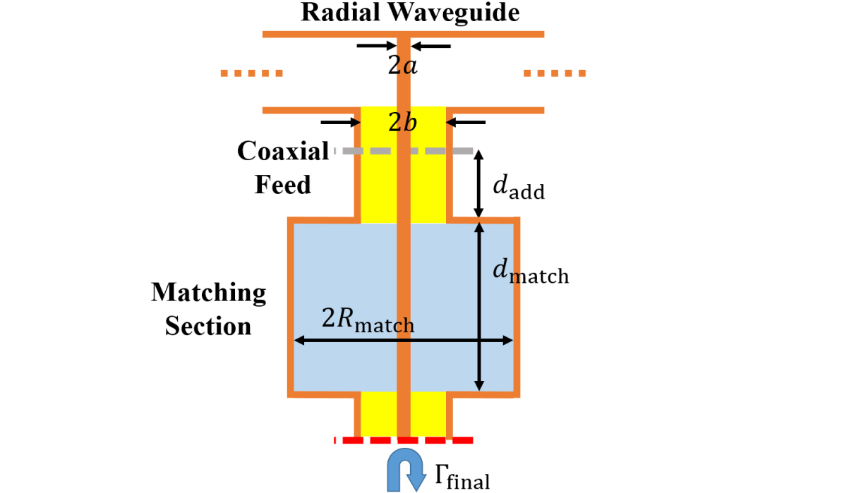
Finally, quarter-wave matching can be performed with the real to minimize the reflection coefficient of the device, . It was achieved by introducing a modified coaxial cable section as shown in Fig. 6(c), then carefully selecting the dielectric permittivity within it, , and optimizing the radius of its outer conductor, , according to the resulting characteristic impedance :
| (54) |
The length of this matching section, , has to be a quarter of the operating wavelength in the presence of the dielectric filling, i.e., , to achieve a perfect match.
This procedure was adopted to design an impedance matching structure for the example beam-shaping shell device. The original reflection coefficient was . The smallest length that renders a real (52) is mm. Nevertheless, this value is not feasible in practice because the resulting matching section will be almost directly connected to the coax-waveguide junction. The resulting evanescent waves generated from the discontinuities of this short matching section would significantly impact the characterization of the coaxial feed. Hence, was selected to be the next possible value, mm, that yield a real . This extra section of coaxial cable has a real reflection coefficient (or dB) and an input impedance . Consequently, the required characteristic impedance of the matching section, given by (54), is . The dielectric material within the matching section of the quarter-wave impedance transformer was selected to be free-space (air). The theoretical formulas (52)-(54) then gave the required dimensions mm and mm, as listed in Table I. With these dimensions, the magnitude of the final reflection coefficient, (or dB) still deviated from a perfect match. This was due to the parasitic effects stemming from the large difference between and the coaxial outer radius .
In order to mitigate these parasitic effects, the dimensions and were optimized. As shown in Table I, the subsequent optimized dimensions mm and mm resulted in a reflection coefficient of (or dB), significantly lower than without the matching network.
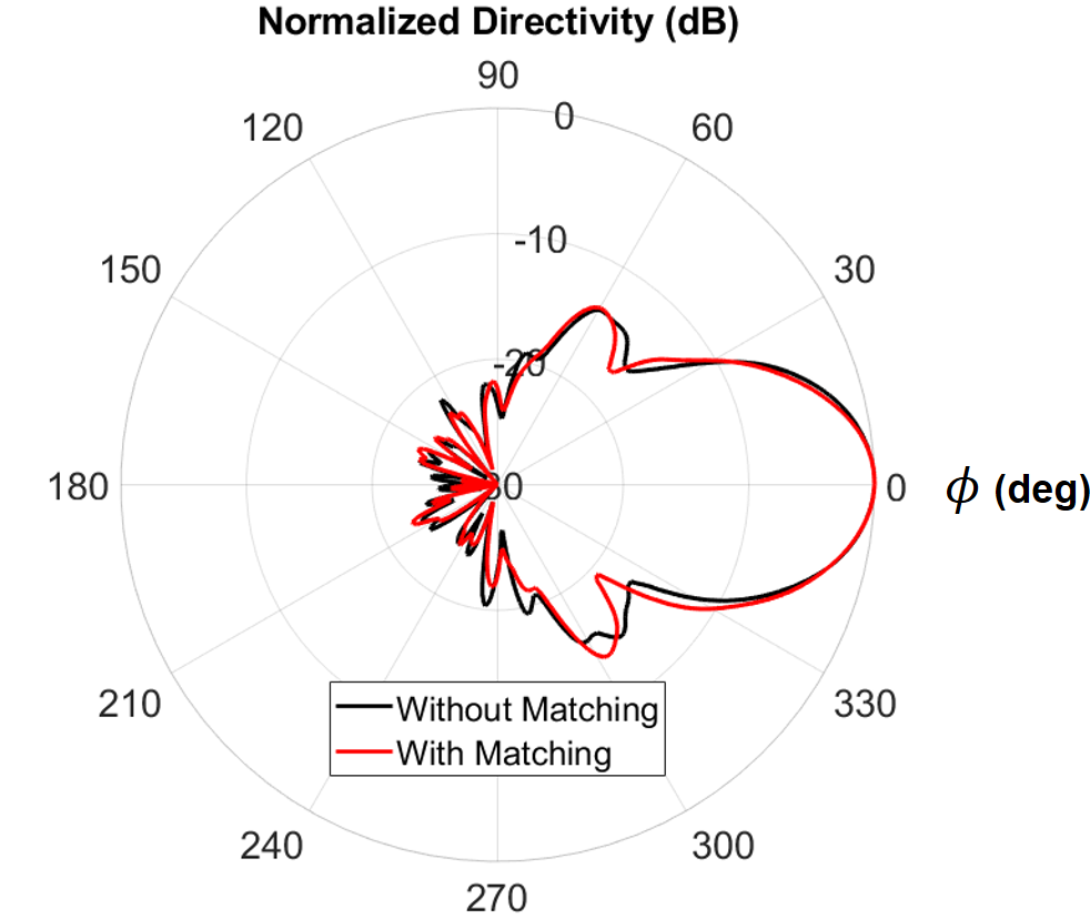
This optimized impedance matching structure was applied to the example beam-shaping shell system. Fig. 7 illustrates the full-wave simulations obtained with Ansys HFSS. Fig. 8 compares the radiation pattern of the original device to that of the impedance matched version. The quarter-wave transformer greatly improved impedance match of the device with only a negligible disturbance in its radiation pattern.
| Initial Design Based on Formulas | Optimized Design | |
|---|---|---|
| 7.5 (mm) | 7.0 (mm) | |
| 4.1 (mm) | 3.3 (mm) | |
| (air) | (air) | |
| 0.198 | 0.088 |
IV Conclusion
In this paper, a rigorous investigation of a set of layered, concentric cylindrical metasurfaces excited by a displaced, off-center coaxial feed in a radial waveguide was presented. By employing the Hankel function addition theorem for all azimuthal orders, the scattering properties of the displaced coaxial feed were obtained efficiently from those of a central coaxial feed. The formulation was used to derive the multimodal -matrix of the displaced coaxial feed. It was then combined with multimodal wave matrix theory, which has been used successfully to model concentric metasurfaces, to realize the design of an arbitrary field transforming structure excited by a displaced coaxial feed. The modeling approach was verified with a beam-shaping shell device which generated a specified narrow radiated beam. Excellent agreement between theoretical predictions and the corresponding full-wave simulations showcased the accuracy of the developed analysis and synthesis method.
Moreover, the practical performance of this example device was significantly enhanced with the design and seamless integration of a quarter-wave impedance transformer into the displaced coaxial feed. This outcome demonstrates that characterizing a realistic coaxial feed not only provides accurate modeling of the feed-metasurface interaction, but it also allows for the design of fully-integrated matching feed networks. Future work includes the characterization of multiple coaxial feeds to realize advanced cylindrical-metasurface-based MIMO devices.
Appendix A Addition Theorem for Hankel Functions of Any Azimuthal Order
The addition theorem for Hankel functions of all azimuthal orders, given by (22) and (23), is derived in detail in this appendix. The proof is based upon the raising and lowering operators discussed in [35] applied to elementary cylindrical waves. Specifically, the raising operator is defined as:
| (55) |
where and represent the rectangular coordinates corresponding to the cylindrical coordinate . By applying (55) on an elementary cylindrical wave of order , which depends on both the radial and azimuthal coordinates, the azimuthal order of the wave is raised by exactly 1, i.e.,
| (56) |
where denotes the solution of the Bessel differential equation of order . Similarly, a lowering operator can be defined such that it lowers the order of an elementary cylindrical waves by 1:
| (57) |
| (58) |
To see why (56) is true, its partial derivatives need to be carried out explicitly. By utilizing the following relationships,
| (59) |
| (60) |
| (61) |
it can be shown that,
| (62) |
The right hand side of (56) follows directly from this equation once the following Bessel function recurrence relation [35, 43] is applied:
| (63) |
Likewise, (58) can also be demonstrated by incorporating another Bessel function recurrence relation:
| (64) |
Now that the raising and lowering operators are defined, the proof of the addition theorem for outgoing cylindrical waves (22) is straightforward. We start from the well-known Hankel function addition theorem for the fundamental mode () [35, 36, 43],
| (65) |
Next, let us apply the following raising operator times to both sides of (65):
| (66) |
where and represent the rectangular coordinates of , the point of interest in Fig. 3 relative to the displaced feed. By definition and denote the rectangular coordinates of the displaced feed. Therefore,
| (67) | ||||||||
When , (65) becomes,
| (68) |
Since the location of the displaced feed is given and fixed, and are constants throughout the analysis. It is now simple using (67) to prove that :
Therefore, the right-hand-side of (68) can be rewritten as:
| (69) |
This relation indicates that the raising operators directly yield,
| (70) |
Finally, by changing the summation variable on the right-hand-side to , the first part () of (22) is proven,
| (71) |
The case of can be also proven by adopting the same procedure. This finishes the proof of the addition theorem for outgoing waves (22).
The addition theorem for incoming waves (23) can be derived directly by complex conjugating (22), i.e.,
| (72) |
Next, by changing the variables and in (72) to and , respectively, leads to,
| (73) |
Then, by utilizing the following property of [43]:
| (74) |
(73) can be rewritten as:
| (75) |
Finally, (23) is proven by cancelling out the on both sides of the equation.
References
- [1] G. Xu, G. V. Eleftheriades, and S. V. Hum, “Discrete-Fourier-transform based framework for analysis and synthesis of cylindrical omega-bianisotropic metasurfaces,” Phys. Rev. Appl., vol. 14, p. 064055, Dec. 2020.
- [2] G. Xu, G. V. Eleftheriades, and S. V. Hum, “Analysis and synthesis of cylindrical omega-bianisotropic metasurfaces with mode expansion,” 2020 IEEE International Symposium on Antennas and Propagation and North American Radio Science Meeting, Montreal, QC, Canada, 2020, pp. 763-764
- [3] C. -W. Lin and A. Grbic, “Field synthesis with azimuthally-varying, cascaded, cylindrical metasurfaces using a wave matrix approach,” IEEE Trans. Antennas Propag., vol. 71, no. 1, pp. 796-808, Jan. 2023.
- [4] C. -W. Lin and A. Grbic, “A wave matrix approach to designing azimuthally-varying cylindrical metasurfaces,” 2021 IEEE International Symposium on Antennas and Propagation and USNC-URSI Radio Science Meeting (APS/URSI), Marina bay Sands, Singapore, 2021, pp. 1857-1858.
- [5] K. -Y. Liu, G. -M. Wang, T. Cai, H. -P. Li and T. -Y. Li, ”Conformal polarization conversion metasurface for omni-directional circular polarization antenna application,” IEEE Trans. Antennas Propag., vol. 69, no. 6, pp. 3349-3358, Jun. 2021.
- [6] C. -W. Lin and A. Grbic, “Analysis and synthesis of cascaded cylindrical metasurfaces using a wave matrix approach,” IEEE Trans. Antennas Propag., vol. 69, no. 10, pp. 6546-6559, Oct. 2021.
- [7] M. Safari, H. Kazemi, A. Abdolali, M. Albooyeh, and F. Capolino, “Illusion mechanisms with cylindrical metasurfaces: A general synthesis approach,” Phys. Rev. B, vol. 100, p. 165418, Oct. 2019.
- [8] P. -Y. Chen and A. Alù, “Mantle cloaking using thin patterned metasurfaces,” Phys. Rev. B, vol. 84, p. 205110, Nov. 2011.
- [9] M. Selvanayagam and G. V. Eleftheriades, “An active electromagnetic cloak using the equivalence principle,” IEEE Antennas Wirel. Propag. Lett., vol. 11, pp. 1226–1229, Oct. 2012.
- [10] M. Selvanayagam and G. V. Eleftheriades, “Experimental demonstration of active electromagnetic cloaking,” Phys. Rev. X, vol. 3, p. 041011, Nov. 2013.
- [11] D. L. Sounas, R. Fleury, and A. Alù, “Unidirectional cloaking based on metasurfaces with balanced loss and gain,” Phys. Rev. Appl., vol. 4, p. 014005, Jul. 2015.
- [12] D. -H. Kwon, “Lossless tensor surface electromagnetic cloaking for large objects in free space,” Phys. Rev. B, vol. 98, p. 125137, Sep. 2018.
- [13] H. Lee and D.-H. Kwon, “Microwave metasurface cloaking for freestanding objects,” Phys. Rev. Appl., vol. 17, p. 054012, May 2022.
- [14] M. Dehmollaian, G. Lavigne, and C. Caloz, “Transmittable nonreciprocal cloaking,” Phys. Rev. Appl., vol. 19, p. 014051, Jan. 2023.
- [15] D.-H. Kwon, “Illusion electromagnetics for free-standing objects using passive lossless metasurfaces,” Phys. Rev. B, vol. 101, p. 235135, Jun. 2020.
- [16] Y. Mazor, “Nonreciprocal guided waves on azimuthally varying cylindrical metasurfaces,” 2022 Sixteenth International Congress on Artificial Materials for Novel Wave Phenomena (Metamaterials), Siena, Italy, 2022, pp. 308–310.
- [17] C. J. M. Barker and A. K. Iyer, “Equivalent surface impedances for below-cutoff propagation in circular waveguides,” 2020 Fourteenth International Congress on Artificial Materials for Novel Wave Phenomena (Metamaterials), New York, NY, USA, 2020, pp. 177–179.
- [18] C. J. M. Barker, N. De Zanche, and A. K. Iyer, “Dispersion and polarization control in below-cutoff circular waveguides using anisotropic metasurface liners,” IEEE Trans. Microw. Theory Tech., vol. 71, no. 8, pp. 3392–3403, Aug. 2023.
- [19] C. -W. Lin, R. W. Ziolkowski and A. Grbic, ”A cylindrical, metasurface-based, azimuthally-symmetric beam-shaping shell,” 2023 17th European Conference on Antennas and Propagation (EuCAP), Florence, Italy, 2023, pp. 1-3.
- [20] J. Li, A. Díaz-Rubio, C. Shen, Z. Jia, S. Tretyakov, and S. Cummer, “Highly efficient generation of angular momentum with cylindrical bianisotropic metasurfaces,” Phys. Rev. Appl., vol. 11, p. 024016, Feb. 2019.
- [21] Y. Mazor and A. Alù, “Angular-momentum selectivity and asymmetry in highly confined wave propagation along sheath-helical metasurface tubes,” Phys. Rev. B, vol. 99, p. 155425, Apr. 2019.
- [22] C. -W. Lin and A. Grbic, ”A realistic coaxial feed for cascaded cylindrical metasurfaces,” IEEE Antennas Wirel. Propag. Lett., vol. 22, no. 11, pp. 2624-2628, Nov. 2023.
- [23] C. -W. Lin and A. Grbic, ”Design of coaxially-fed, concentrically-cascaded, cylindrical metasurfaces,” 2022 IEEE International Symposium on Antennas and Propagation and USNC-URSI Radio Science Meeting (AP-S/URSI), Denver, CO, USA, 2022, pp. 1886-1887.
- [24] T. J. Smy, S. A. Stewart and S. Gupta, ”Eigenfunction expansion (EFE) analysis of cylindrical metasurfaces—Part I: Zero thickness tensorial surface susceptibility model,” IEEE Trans. Microw. Theory Tech, vol. 71, no. 8, pp. 3352-3365, Aug. 2023.
- [25] T. J. Smy and S. Gupta, ”Eigenfunction expansion (EFE) analysis of cylindrical metasurfaces—Part II: Sectors and multishells,” IEEE Trans. Microw. Theory Tech, vol. 71, no. 8, pp. 3366-3378, Aug. 2023.
- [26] T. J. Smy, S. A. Stewart, J. G. N. Rahmeier and S. Gupta, ”Eigenfunction analysis of cylindrical metasurfaces with complete tensorial surface susceptibilities,” 2022 IEEE International Symposium on Antennas and Propagation and USNC-URSI Radio Science Meeting (AP-S/URSI), Denver, CO, USA, 2022, pp. 459-460.
- [27] S. Sandeep and S. Y. Huang, ”Simulation of circular cylindrical metasurfaces using GSTC-MoM,” IEEE J. Multiscale Multiphysics Comput. Tech., vol. 3, pp. 185-192, Nov. 2018.
- [28] S. Sandeep, A. Gasiewski, and A. F. Peterson, “Application of cylindrical IE-GSTC to physical metasurfaces,” J. Electromagn. Waves Appl., vol. 37, no. 14, pp. 1162–1186, Jul. 2023.
- [29] Z. Šipuš, Z. Eres, and D. Barbarić, “Modeling cascaded cylindrical metasurfaces with spatially-varying impedance distribution,” Radioengineering, vol. 27, pp. 505–511, Sep. 2019.
- [30] Z. Shen, J. L. Volakis and R. H. MacPhie, “A coaxial-radial line junction with a top loading disk for broadband matchings,” Microw. Opt. Technol. Lett., vol. 22, no. 2, pp. 87-90, Jul. 1999.
- [31] J. D. Heebl, M. Ettorre, and A. Grbic, “Wireless links in the radiative near field via Bessel beams,” Phys. Rev. Appl., vol. 6, p. 034018, Sep. 2016.
- [32] F. Alsolamy and A. Grbic, “Antenna aperture synthesis using mode-converting metasurfaces,” IEEE Open J. Antennas Propag., vol. 2, pp. 726-737, Jun. 2021.
- [33] G. V. Eleftheriades, A. S. Omar, L. P. B. Katehi and G. M. Rebeiz, “Some important properties of waveguide junction generalized scattering matrices in the context of the mode matching technique,” IEEE Trans. Microw. Theory Tech., vol. 42, no. 10, pp. 1896-1903, Oct. 1994.
- [34] E. Kühn, “A mode-matching method for solving field problems in waveguide and resonator circuits”, Arch. Elektron. Übertrag., vol. 27, pp. 511-513, Dec. 1973.
- [35] W. C. Chew, Waves and Fields in Inhomogenous Media. New York, NY, USA: Wiley-IEEE Press, 1995.
- [36] P. A. Martin, Multiple Scattering: Interaction of Time-Harmonic Waves with N Obstacles. Cambridge, UK: Cambridge University Press, 2006.
- [37] D. M. Pozar, Microwave Engineering, 4th ed. New York, NY, USA: Wiley, 2012.
- [38] M. Ettorre, S. M. Rudolph and A. Grbic, “Generation of propagating Bessel beams using leaky-wave modes: Experimental validation,” IEEE Trans. Antennas Propag., vol. 60, no. 6, pp. 2645-2653, Jun. 2012.
- [39] K. Kurokawa, “Power waves and the scattering matrix,” IEEE Trans. Microw. Theory Tech., vol. MTT-13, no. 2, pp. 194–202, Mar. 1965.
- [40] T. -T. Lu and S. -H. Shiou, ”Inverses of 2 × 2 block matrices,” Comput. Math. Appl., vol. 43, pp. 119-129, Jan. 2002.
- [41] S. Arslanagić and R. W. Ziolkowski, “Highly subwavelength, superdirective cylindrical nanoantenna,” Phys. Rev. Lett., vol. 120, p. 237401, Jun. 2018.
- [42] R. W. Ziolkowski, “Mixtures of multipoles — Should they be in your EM toolbox?,” IEEE Open J. Antennas Propag., vol. 3, pp. 154-188, 2022.
- [43] R. F. Harrington, Time-Harmonic Electromagnetic Fields. Piscataway, NJ, USA: IEEE-Press, 2001.