Exact and universal quantum Monte Carlo estimators
for energy susceptibility and fidelity susceptibility

Abstract

We derive exact, universal, closed-form quantum Monte Carlo estimators for finite temperature energy susceptibility and fidelity susceptibility for essentially arbitrary Hamiltonians. We demonstrate how our method can be used to study quantum phase transitions without knowledge of an order parameter and without the need to design system-specific ergodic quantum Monte Carlo update rules by applying it to a class of random models.

Introduction.—Traditionally, quantum phase transitions (QPTs) are analyzed using order parameters Sachdev (2011). Informally, an order parameter is a model-specific measurement that experiences a sharp jump at the interface of two quantum phases, also known as a quantum critical point. However for an unknown system, designing an order parameter may not be obvious. There has thus been a growing effort to develop order-parameter free techniques to detect QPTs. The fidelity paradigm Gu (2010), which has taken central stage in recent years, is based on the observation that fidelity across phase boundaries is exponentially suppressed Zanardi and Paunković (2006); Zanardi et al. (2007a, b, c).

In many cases, it is sufficient to compute only the second-order term in the Taylor expansion of fidelity, known as fidelity susceptibility (FS) You et al. (2007). Though there are examples where it is known to fail Cincio et al. (2019), the FS has known scaling relations to several important thermodynamic quantities Gu et al. (2008); Gu and Lin (2009); Gu and Yu (2014); Quan et al. (2006) including the energy susceptibility (ES) Chen et al. (2008); Campos Venuti and Zanardi (2007), or the second derivative of the groundstate energy. Beyond exactly solvable models, one can compute FS numerically for small systems using Lanczos-Arnoldi You et al. (2007); Rigol et al. (2009); Kasatkin et al. (2024), for large systems with bounded entanglement using tensor networks Sun et al. (2015); Kasatkin et al. (2024); Zhou et al. (2008); Jiang et al. (2011); Jordan et al. (2009); Wang et al. (2010), and for systems where the groundstate can be repeatedly measured (numerically or experimentally) using machine learning Kasatkin et al. (2024). In practice, these techniques rely on model-specific prior information, such as known symmetries .

For general large-scale quantum many-body systems, quantum Monte Carlo (QMC) techniques remain the only viable approach Schwandt et al. (2009); Albuquerque et al. (2010); Wang et al. (2015). However, most QMC libraries are designed for specific systems (see, e.g., Ref. Bauer et al. (2011)) because the underlying algorithms rely on system-specific update rules. Furthermore, the state-of-the-art QMC FS estimator Wang et al. (2015) assumes the system Hamiltonian is partitioned into a purely diagonal term and a purely off-diagonal driving term. These limitations make applying current QMC methods to unstructured systems without prior knowledge challenging or even impossible.

In this work, we propose universal, exact, closed-form QMC estimators for ES and FS that can be applied to essentially arbitrary Hamiltonians with arbitrary bi-partitioning, without the need to use prior additional knowledge such as known symmetries. We illustrate the power of our method by successfully applying our estimators to randomly generated 100–spin Hamiltonians that do not have a simple geometry and are nonlocal.

To achieve the above, we derive our estimators within the recently proposed permutation matrix representation (PMR) QMC framework Albash et al. (2017); Gupta et al. (2020a). This is for two reasons. First, the PMR-QMC framework writes QMC weights in terms of so-called divided differences, which are amenable to exact and generic derivations. Consequently, our estimators are as general as possible and apply to arbitrarily complicated driving terms that can contain both diagonal and off-diagonal contributions. Second, the PMR-QMC framework allows for the general treatment of entire classes of Hamiltonians. In particular, a recent study Barash et al. (2024) devised an algorithm to automatically compute PMR-QMC update rules that are ergodic and satisfy detailed balance, for arbitrary spin-1/2 Hamiltonians, obviating the need to design system-specific QMC updates. The same method has recently been generalized to apply to the Bose-Hubbard model on arbitrary graphs Akaturk and Hen (2024) and it can be shown to naturally generalize to higher spin systems, arbitrary bosonic and fermionic systems, and mixtures thereof Babakhani et al. (2024).

Thus, our derivations here, together with the existing PMR-QMC framework Barash et al. (2024); Akaturk and Hen (2024); Babakhani et al. (2024), allow us to compute the ES or FS on essentially arbitrarily constructed systems (i.e., any system that can be studied using PMR-QMC) with arbitrary driving terms. This elevates PMR-QMC to a “black-box” algorithm in the study of QPTs. (It should be emphasized, however, that this black box is still subject to the usual obstructions to convergence, such as frustration or the sign problem Hen (2021).)

Numerical demonstration.—Before deriving our estimators, we first demonstrate their success on a class of models where exact results can be computed. Firstly, we study the two-spin model

$$H(\lambda)=Z_{1}Z_{2}+0.1(X_{1}+X_{2})+\lambda(Z_{1}+Z_{2})\,,$$ (1)

where $\{X_{j},Z_{j}\}$ are the Pauli operators acting on the $j^{\text{th}}$ spin. The phases of this model in an NMR system were studied in Ref. Zhang et al. (2008) via a fidelity approach. Unlike most conventionally studied QPTs, such as the transverse-field Ising model, this model has a driving term $H_{1}=Z_{1}+Z_{2}$, which is neither the entire diagonal nor the entire off-diagonal part of $H$ since the static term is $H_{0}=Z_{1}Z_{2}+0.1(X_{1}+X_{2})$. As such, it does not fit into the framework assumed in existing studies (e.g., Ref. Wang et al. (2015)). Nevertheless, it is designed to have critical points at around $\lambda\approx\pm 1$ where an avoided level crossing occurs, and it is anyway small enough to compute the FS by direct diagonalization.

The output of our PMR-QMC FS estimator for different inverse temperatures is shown in Fig. 1. As expected, the curves grow sharper and approach the $T=0$ FS as $T\rightarrow 0$ (i.e., as $\beta\equiv 1/T\rightarrow\infty)$, in agreement with the general relation between Gibbs state FS and groundstate FS. Fitting the peak location of each curve as a function of $T$ to a line, the fitted $T=0$ peak occurs at $\pm 0.98\pm 0.04$, in alignment with the known critical points. Finally, we find $\chi_{F}^{\beta=20}$ is an excellent approximation to the $T=0$ FS, which we will utilize in our next numerical demonstrations.

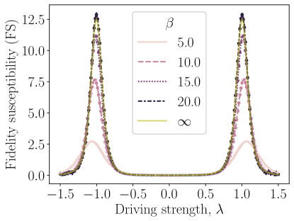
Figure 1: FS for the two spin model, Eq. (1), considered in Ref. Zhang et al. (2008) for different inverse temperatures, $\beta$. Data from QMC are points with 95% confidence intervals from bootstrapping over 5 independent random seeds, whereas direct numerical calculations are shown as lines.

Next, we consider a large ensemble of Hamiltonians generated by random rotations of Eq. (1). In more detail, we generate 10 random unitaries $U_{i}$ such that each $H_{U_{i}}\equiv U_{i}H(\lambda)U_{i}^{\dagger}$ (i) is a 100–spin Hamiltonian with non-trivial support on every spin, (ii) has hundreds of Pauli terms (iii) is efficient to generate and store, and (iv) does not have a severe sign problem. Despite now being 100–spin models, observables agree exactly with the original two spin model by unitary invariance, and hence, we can still validate the results of our QMC algorithm. In addition, existing approaches cannot estimate FS since each $H_{U_{i}}$ is a random model with a random driving term, $U_{i}H_{1}U_{i}$.

Before presenting the results, we provide a brief overview of how such a special ensemble of unitaries was generated, with full details available in Appendix A. Firstly, for $n$ spins, the largest possible set of anti-commuting Paulis is $2n+1$, and there exists an $O(n)$ algorithm to generate such a maximal set Sarkar and Berg (2019). Secondly, $\sum_{i=1}^{L}c_{i}Q_{i}$ is unitary whenever $\{Q_{i}\}_{i=1}^{L}$ is a set of anti-commuting Paulis and $\bm{c}\in\mathds{R}^{L}$ such that $||\bm{c}||_{2}=1$ (for a slight generalization, see Ref. Izmaylov et al. (2020)). Lastly, within PMR-QMC bar ; Barash et al. (2024), it is possible to track the empirical sign of the QMC weight. Together, these facts enable the generation of such a remarkable ensemble.

For each $U_{i}$, the driving term, $U_{i}H_{1}U_{i}^{\dagger}$, typically contains around 100 random Pauli terms of various weights from 1 to 100. Nevertheless, our PMR-QMC estimators consistently show excellent agreement with exact numerical results for observables such as the imaginary-time correlator $G(\tau)$, the ES, and the FS, as shown in Fig. 2. Furthermore, our results confirm established characteristics of these observables; for instance, $G(\tau)$ exhibits symmetry about $\beta/2$, while $\tau G(\tau)$ breaks this symmetry (see Fig. 1 in Ref. Albuquerque et al. (2010) and Fig. 7 in Ref. Wang et al. (2015)). Finally, the ES serves as a robust estimator for quantum criticality in this model, consistent with the general relation between ES and FS discussed in Ref. Albuquerque et al. (2010).

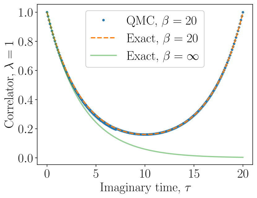
(a) The imaginary time correlator, $G(\tau)$, has the expected symmetry around $\beta/2=10.$

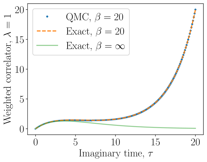
(b) The weighted imaginary time correlator, $\tau G(\tau)$, breaks the $\beta/2$ symmetry as expected.

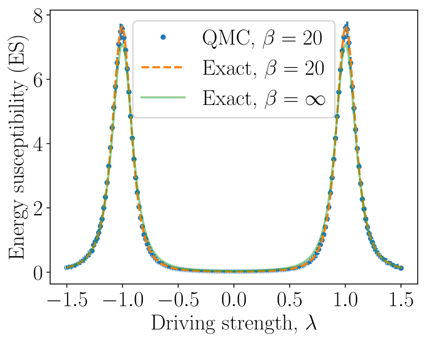
(c) The ES correctly predicts critical points despite $\beta=20$ curve not quite converging to $\beta=\infty$ curve.

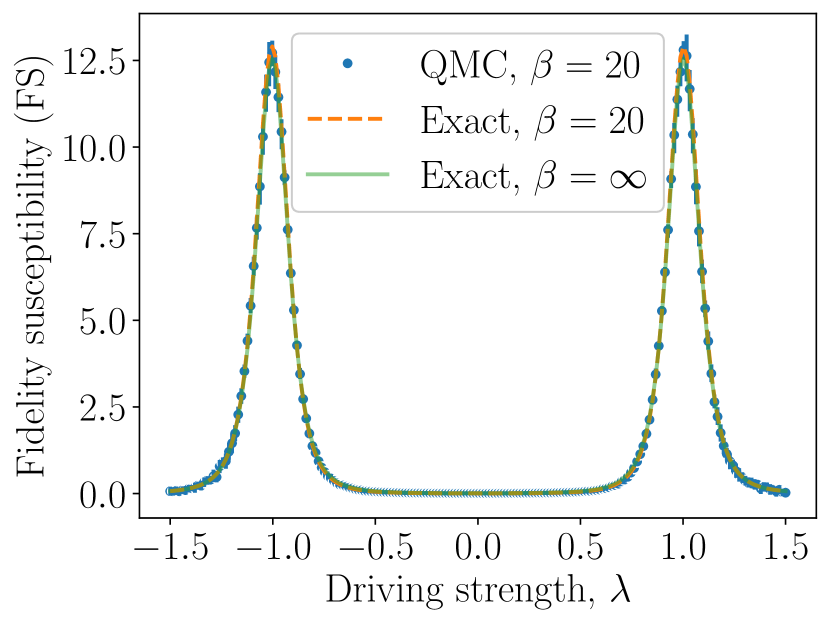
(d) The FS correctly predicts critical points more sharply than ES, and $\beta=20$ curve matches $\beta=\infty$ curve.

Figure 2: Comparison of QMC estimates with exact values for an ensemble of 100–spin Hamiltonians generated by random rotations of Eq. (1). Detailed information on the ensemble can be found in Appendix A and is summarized in the main text. QMC estimates include 95% confidence intervals across 10 models, where each calculation employs a different random seed. In all cases, the QMC estimates show excellent agreement with exact finite $\beta$ curves.

Definitions and background.— To state and prove our estimators, we first define the ES and FS. Throughout, we assume $H(\lambda)=H_{0}+\lambda H_{1}$ is a single parameter family of Hamiltonians, where $H_{1}$ is the driving term. We denote by $\mathcal{Z}$ the partition function $\mathcal{Z}=\Tr[e^{-\beta H}]$ for inverse temperature $\beta\equiv 1/T$, so the thermal average of an observable $O$ is $\langle O\rangle=\Tr[Oe^{-\beta H}]/\mathcal{Z}$. We denote $H_{1}(\tau)\equiv e^{\tau H}H_{1}e^{-\tau H}$ as the imaginary time evolved $H_{1}$ with the corresponding imaginary time correlator $G(\tau;\beta,\lambda)\equiv\langle H_{1}(\tau)H_{1}\rangle-\langle H_{1}\rangle^{2}.$

The ES is the second derivative of the ground state energy with respect to $\lambda$. However, because QMC methods inherently operate at finite temperature, we consider instead the second derivative of the free energy, i.e., of $(-1/\beta)\ln\mathcal{Z}$, which can be expressed as Albuquerque et al. (2010)

$$\chi_{E}^{\beta}(\lambda;\beta)\equiv\int_{0}^{\beta}G(\tau;\beta,\lambda)\mathrm{d}\tau,$$ (2)

Similarly, the FS between two Gibbs states at finite temperature can be written as Albuquerque et al. (2010); Wang et al. (2015); Schwandt et al. (2009)

$$\chi^{\beta}_{F}(\lambda;\beta)\equiv\int_{0}^{\beta/2}\tau G(\tau;\beta,\lambda)\mathrm{d}\tau.$$ (3)

Both Eq. (2) and Eq. (3) tend to their zero temperature counterparts for $\beta\rightarrow\infty$. Therefore, for simplicity, we refer to these as the ES and FS henceforth. It is well-known that these two quantities are closely related Chen et al. (2008); Campos Venuti and Zanardi (2007). In numerical simulations, the FS is a sharper indicator of QPTs, albeit at the expense of being more computationally intensive Albuquerque et al. (2010).

We next briefly summarize PMR-QMC Gupta et al. (2020a). To begin, we write the Hamiltonian in PMR form Ezzell and Hen (2024), $H(\lambda)=D_{0}(\lambda)+\sum_{j=1}^{M}D_{j}(\lambda)P_{j},$ where $D_{j}$ are diagonal matrices and $\{P_{j}\}_{j=1}^{M}$ are permutation matrices that are a subset of a special Abelian group, $G$ . For spin-1/2 systems, $G$ consists of all Pauli-X strings Barash et al. (2024). Practically useful $G$ have also been devised for higher spin models Babakhani et al. (2024), Bose-Hubbard models Akaturk and Hen (2024), flux superconducting circuits Halverson et al. (2020), and in principle, every square matrix can be written in PMR form for some suitable $G$ Ezzell and Hen (2024).

A non-trivial though useful consequence is that we can write the partition function as a sum of generalized Boltzmann weights Albash et al. (2017); Gupta et al. (2020a); Barash et al. (2024) $\mathcal{Z}=\sum_{\cal C}w_{\mathcal{C}}$, where each $\mathcal{C}=(z,S_{\bm{i}_{q}})$ is a QMC configuration, and each weight $w_{\cal C}=D_{(z,S_{\bm{i}_{q}})}e^{-\beta[E_{z_{0}},\ldots,E_{z_{q}}]}$ is efficiently computable Gupta et al. (2020b). A derivation is provided in Ref. Gupta et al. (2020a). Here, we provide only a brief summary. Most importantly, a PMR-QMC estimator $O_{\mathcal{C}}$ is a function of $\mathcal{C}$ such that

$$\langle O\rangle=\frac{\sum_{\mathcal{C}}w_{\mathcal{C}}O_{\mathcal{C}}}{\sum_{\mathcal{C}}w_{\mathcal{C}}}.$$ (4)

Here, $S_{\bm{i}_{q}}\equiv P_{\bm{i}_{q}}\ldots P_{\bm{i}_{1}}$ denote a product of $q$ permutations, each from $\{P_{j}\}_{j=1}^{M}$. The summation over $\cal C$ should be interpreted as a double sum over all basis states $\ket{z}$ and all possible products $S_{\bm{i}_{q}}$ evaluating to the identity, for $q$ from $0$ to $\infty$. Next, we denote $\ket{z_{0}}\equiv\ket{z}$ and $\ket{z_{k}}\equiv P_{\bm{i}_{k}}\ldots P_{\bm{i}_{1}}\ket{z}$. This lets us define the “diagonal-energies” as $E_{z_{k}}\equiv\langle z_{k}|H|z_{k}\rangle=\langle z_{k}|D_{0}|z_{k}\rangle$ and the off-diagonal “hopping strength,” $D_{(z,S_{\bm{i}_{q}})}\equiv\prod_{k=1}^{q}\langle z_{k}|D_{i_{k}}|z_{k}\rangle.$ In practice, both can be efficiently computed with a look-up table Albash et al. (2017); Gupta et al. (2020a). Finally, $e^{-\beta[E_{z_{0}},\ldots,E_{z_{q}}]}$ is a divided difference of the exponential, which plays a key role in the derivation of our estimators, so we now discuss it in more detail.

The divided difference of any holomorphic function $f(x)$ over a multiset $[x_{0},\ldots,x_{q}]$ can be defined as $f[x_{0},\ldots,x_{q}]\equiv(1/(2\pi i))\oint\limits_{\Gamma}{f(x)}/{\prod_{i=0}^{q}(x-x_{i})}\mathrm{d}x,$ for $\Gamma$ a positively oriented contour enclosing all the $x_{i}^{\prime}s$ McCurdy et al. (1984). Well-known elementary definitions and properties of the divided difference follow by direct application of the residue theorem McCurdy et al. (1984). Another important property that follows is the Leibniz rule de Boor (2005),

$$(f\cdot g)[x_{0},\ldots,x_{q}]=\sum_{j=0}^{q}f[x_{0},\ldots,x_{j}]g[x_{j},\ldots,x_{q}].$$ (5)

As in Refs. Albash et al. (2017); Gupta et al. (2020a, b); Barash et al. (2024), we adopt the shorthand notation $e^{t[x_{0},\ldots,x_{q}]}\equiv f[x_{0},\ldots,x_{q}]$, where $f(x)=e^{tx}$. Replacing the variable $x\rightarrow\alpha x$ in the contour integral definition, we find, $\alpha^{q}e^{t[\alpha x_{0},\ldots,\alpha x_{q}]}=e^{\alpha t[x_{0},\ldots,x_{q}]}$. Combining this with Eq. (11) of Ref. Kunz (1965) with $P_{m}(x)=1$, we get,

$$\mathcal{L}\left\{e^{\alpha t[x_{0},\ldots,x_{q}]}\right\}=\frac{\alpha^{q}}{\prod_{j=0}^{q}(s-\alpha x_{j})},$$ (6)

where $\mathcal{L}$ denotes the Laplace transform from $t\rightarrow s$. This can also be shown explicitly by expanding $e^{\alpha tx}$ within the contour integral definition of the divided difference.

Pure diagonal derivations.— For simplicity, first suppose the driver is purely diagonal, i.e., $D_{0}=\lambda H_{1}$ (recall $H(\lambda)=H_{0}+\lambda H_{1}=D_{0}+\sum_{j}D_{j}(\lambda)P_{j}$). Following Eq. (24) in Barash et al. (2024), we can immediately write

$$(D_{0})_{\mathcal{C}}=E_{z},$$ (7)

which can be used to evaluate $\langle D_{0}\rangle^{2}$. Since this does not depend on $\tau$, subsequent integrations are straightforward, i.e., $\int_{0}^{\beta}\langle D_{0}\rangle^{2}\mathrm{d}\tau=\beta\langle D_{0}\rangle^{2}$. Hence, all the work in deriving $G(\tau)$ and integrals thereof is in the imaginary time two-point correlator, $\langle D_{0}(\tau)D_{0}\rangle$.

To proceed, we first observe $\mathcal{Z}\langle D_{0}(\tau)D_{0}\rangle=\sum_{z}\langle z|D_{0}e^{-\tau H}D_{0}e^{-(\beta-\tau)H}|z\rangle.$ Applying the Leibniz rule from right to left on the PMR expansions of the two exponentials, we find,

$$(D_{0}(\tau)D_{0})_{\mathcal{C}}=\\ \frac{E_{z}}{e^{-\beta[E_{z_{0}},\ldots,E_{z_{q}}]}}\sum_{j=0}^{q}E_{z_{j}}e^{-\tau[E_{z_{j}},\ldots,E_{z_{q}}]}e^{-(\beta-\tau)[E_{z_{0}},\ldots,E_{z_{j}}]}.$$ (8)

Note that the denominator of $e^{-\beta[E_{z_{0}},\ldots,E_{z_{q}}]}$ comes from multiplying by $e^{-\beta[E_{z_{0}},\ldots,E_{z_{q}}]}/e^{-\beta[E_{z_{0}},\ldots,E_{z_{q}}]}$ to coax the expression into a PMR-QMC estimator as is done in Ref. Barash et al. (2024). Combining Eqs. (7) and (8), we have an explicit estimator for $G(\tau).$

Since the $\tau$ dependence is entirely contained in the divided differences in Eq. (8), we now prove Theorem 1.

Theorem 1 (Energy susceptibility integral).

$$\int_{0}^{\beta}e^{-\tau[x_{j},\ldots,x_{q}]}e^{-(\beta-\tau)[x_{0},\ldots,x_{j}]}\mathrm{d}\tau=-e^{-\beta[x_{0},\ldots,x_{q},x_{j}]}.$$ (9)

Proof.

Let $f(t)=e^{-t[x_{j},\ldots,x_{q}]}$ and $g(t)=e^{-t[x_{0},\ldots,x_{j}]}$. Now, the left side can be written as the convolution $(f*g)(\beta)$. Since $\mathcal{L}\left\{f*g\right\}=\mathcal{L}\left\{f\right\}\mathcal{L}\left\{g\right\}$ holds for the Laplace transform, Eq. (6) leads to the claimed result. ∎

As a consequence, we have derived the estimator,

Corollary 1 (Energy susceptibility estimator).

$$\left(\int_{0}^{\beta}D_{0}(\tau)D_{0}\ \mathrm{d}\tau\right)_{\mathcal{C}}=\\ \frac{-E_{z}}{e^{-\beta[E_{z_{0}},\ldots,E_{z_{q}}]}}\sum_{j=0}^{q}E_{z_{j}}e^{-\beta[E_{z_{0}},\ldots,E_{z_{q}},E_{z_{j}}]},$$ (10)

which gives an estimator for $\chi_{E}^{\beta}$ (see Eq. (2)) when combined with Eq. (7).

To extend this result to $\chi_{F}^{\beta}$, we first prove,

Lemma 1 (Sum over repeated arguments).

$$\tau e^{-\tau[x_{0},\ldots,x_{j}]}=-\sum_{m=0}^{j}e^{-\tau[x_{0},\ldots,x_{j},x_{m}]}$$ (11)

Proof.

Let $f(\tau)\equiv e^{-\tau[x_{0},\ldots,x_{j}]}$. From Laplace transform properties, Eq. (6), and algebra, $\mathcal{L}\left\{\tau f(\tau)\right\}=-\partial_{s}\mathcal{L}\left\{f(\tau)\right\}=\mathcal{L}\left\{-\sum_{m=0}^{j}e^{-\tau[x_{0},\ldots,x_{j},x_{m}]}\right\}.$ Inverting the Laplace transform, we get the claimed equality. ∎

Combined with our earlier results, we can now prove Theorem 2, which gives an estimator for $\chi_{F}^{\beta}$.

Theorem 2 (Fidelity susceptibility integral).

$$\int_{0}^{\beta/2}\tau e^{-\tau[x_{j},\ldots,x_{q}]}e^{-(\beta-\tau)[x_{0},\ldots,x_{j}]}\mathrm{d}\tau=\\ \sum_{r=0}^{j}e^{-\frac{\beta}{2}[x_{0},\ldots,x_{r}]}\sum_{m=j}^{q}e^{-\frac{\beta}{2}[x_{r},\ldots,x_{q},x_{j},x_{m}]}$$ (12)

Proof.

Our strategy is to coax the integrand into $e^{-\tau[x_{j},\ldots,x_{q},x_{m}]}e^{-(\frac{\beta}{2}-\tau)[x_{r},\ldots,x_{j}]}$, whereupon we can use Theorem 1 with the substitution $\beta\rightarrow\beta/2.$ Firstly, it follows from Eq. (5) that $e^{-(\beta-\tau)[x_{0},\ldots,x_{j}]}=\sum_{r=0}^{j}e^{-(\beta/2)[x_{0},\ldots,x_{r}]}e^{-(\beta/2-\tau)[x_{r},\ldots,x_{j}]}$ because $e^{-(\beta-\tau)x}=e^{-(\beta/2)x}e^{-(\beta/2-\tau)x}$. Employing Lemma 1, we can remove the linear $\tau$ at the expense of summing over repeated entries $m=j$ to $m=q$. Together, the integrand is now of the desired form to use Theorem 1. ∎

Immediately by Theorem 2, we get the estimator,

Corollary 2 (Fidelity susceptibility estimator).

$$\left(\int_{0}^{\beta/2}\tau D_{0}(\tau)D_{0}\mathrm{d}\tau\right)_{\mathcal{C}}=\frac{E_{z}}{e^{-\beta[E_{z_{0}},\ldots,E_{z_{q}}]}}\sum_{j=0}^{q}E_{z_{j}}\\ \times\sum_{r=0}^{j}e^{-\frac{\beta}{2}[E_{z_{0}},\ldots,E_{z_{r}}]}\sum_{m=j}^{q}e^{-\frac{\beta}{2}[E_{z_{r}},\ldots,E_{z_{q}},E_{z_{j}},E_{z_{m}}]}$$ (13)

which gives an estimator for $\chi_{F}^{\beta}$ (see Eq. (3)) when combined with Eq. (7).

On complexity of estimators.— When evaluating an estimator in PMR-QMC, we have $O(1)$ access to each $E_{z}$ and to $\exp{-\beta[E_{z},\ldots,E_{z_{q}}]}$ Gupta et al. (2020a); Barash et al. (2024), but evaluating the divided difference with the addition or removal of an input has an $O(q)$ cost Gupta et al. (2020b). As such, evaluating $(D_{0})_{\mathcal{C}}=E_{z}$ is $O(1)$ but $(D_{0}(\tau)D_{0})_{\mathcal{C}}$ is $O(q^{2})$, so our estimator for $G(\tau)$ is $O(q^{2})$. Similarly, the ES estimator is also $O(q^{2})$, but the FS estimator is $O(q^{4})$. Since we expect $\langle q\rangle\propto\beta$ for many systems Albash et al. (2017), the FS estimate becomes costly as $\beta$ is increased. Nevertheless, we expect the total simulation time to be determined by the complexity of QMC updates rather than that of the estimators for a wide range of temperatures. The number of times the estimators are sampled can be made much smaller than the number of QMC updates to reduce auto-correlation, without compromising the accuracy of calculations Landau and Binder (2015).

Pure off-diagonal derivations.— We next suppose the driver is purely off-diagonal, i.e., $\lambda H_{1}=H(\lambda)-D_{0}$. This case reduces to the pure diagonal case with a small, constant overhead. We briefly summarize why here, and additional details are contained in Appendix B for interested readers. Firstly, we know $(D_{0})_{\mathcal{C}}$ from the diagonal case, and we know $(H)_{\mathcal{C}}$ from Eq. (20) of Ref. Barash et al. (2024). Together, we thus know $(H_{1})_{\mathcal{C}}.$ By straightforward manipulations, $(H_{1}(\tau)H_{1})_{\mathcal{C}}=((H^{2})_{\mathcal{C}}+(D_{0}(\tau)D_{0})_{\mathcal{C}}-2(D_{0}H)_{\mathcal{C}})/\lambda^{2}$, and $(H^{2})_{\mathcal{C}}$ is given by Eq. (23) in Ref. Barash et al. (2024), whereas $(D_{0}H)_{\mathcal{C}}=\langle z|D_{0}|z\rangle(H)_{\mathcal{C}}$. Since the only non-trivial $\tau$ dependence is contained in $(D_{0}(\tau)D_{0})_{\mathcal{C}}$, we can write estimators for the ES and FS using the pure diagonal results.

General case—In general, $H_{1}$ may contain both diagonal and off-diagonal terms, but we can always write, $H_{1}=\sum_{l=0}^{R-1}\overline{C}_{l}P_{l}\equiv\sum_{l=0}^{R-1}C_{l}D_{l}P_{l}$ for $C_{l}$ diagonal matrices and $D_{l}P_{l}$ directly from the PMR form of $H$ (see Appendix C for justification). By linearity, $\langle H_{1}\rangle=\sum_{l}\langle\overline{C}_{l}P_{l}\rangle$, so it is sufficient to derive an estimator for individual terms, $(\overline{C}_{l}P_{l})_{\mathcal{C}}.$ By direct PMR-QMC manipulations (see Sec. V.B in Ref. Barash et al. (2024)), we find

$$(\overline{C}_{l}P_{l})_{\mathcal{C}}=\delta_{P_{l}}^{(q)}\frac{C_{l}(z)e^{-\beta[E_{z_{0}},\ldots,E_{z_{q-1}}]}}{e^{-\beta[E_{z_{0}},\ldots,E_{z_{q}}]}},$$ (14)

where $\delta_{P_{l}}^{(q)}$ equals $1$ if the $q^{\text{th}}$ or final permutation in $S_{\bm{i}_{q}}$ is $P_{l}$ and is $0$ otherwise, and we have used the shorthand $\overline{C}_{l}(z)\equiv\langle z|\overline{C}_{l}|z\rangle.$ We retain the use of the $\delta$ function as in Ref. Barash et al. (2024) for simplicity, but we remark that improved statistics can be obtained using indicator functions as explained in Ref. Ezzell and Hen (2024) and used in Ref. bar .

Similarly, we can derive an estimator for $\langle H_{1}(\tau)H_{1}\rangle$ by finding one for $((\overline{C}_{k}P_{k})(\tau)\overline{C}_{l}P_{l})_{\mathcal{C}}.$ In expanding the trace, we encounter a matrix element $\langle z|\overline{C}_{k}P_{k}e^{-\tau H}\overline{C}_{l}P_{l}e^{-(\beta-\tau)H}|z\rangle.$ Using the same Leibniz rule trick as used in Eq. (8) but with the added complexity of enforcing permutations in $S_{\bm{i}_{q}}$ match $P_{l}$ and $P_{k}$ in appropriate places as in Eq. (14), we find

$$((\overline{C}_{k}P_{k})(\tau)\overline{C}_{l}P_{l})_{\mathcal{C}}=\frac{\delta_{P_{k}}^{(q)}\overline{C}_{k}(z)}{e^{-\beta[E_{z_{0}},\ldots,E_{z_{q}}]}}\times\\ \sum_{j=1}^{q-1}\delta^{(j)}_{P_{l}}\overline{C}_{l}(z_{j})e^{-\tau[E_{z_{j}},\ldots,E_{z_{q-1}}]}e^{-(\beta-\tau)[E_{z_{0}},\ldots,E_{z_{j-1}}]}.$$ (15)

Although the presence of $P_{k}$ and $P_{l}$ cause $e^{-(\beta-\tau)[\cdots]}$ to miss $E_{z_{j}}$ and $e^{-\tau[\cdots]}$ to miss $E_{z_{q}}$ compared to Eq. (8), this estimator still has the same product $e^{-(\beta-\tau)[\cdots]}e^{-\tau[\cdots]}$, so our divided difference lemmas and theorems still apply.

As such, we have derived susceptibility estimators for arbitrary partitions of $H$ into $H_{0}$ and $H_{1}$. For example,

$$\left(\int_{0}^{\beta/2}\tau(\overline{C}_{k}P_{k})(\tau)\overline{C}_{l}P_{l}\ \mathrm{d}\tau\right)_{\mathcal{C}}=\frac{\delta_{P_{k}}^{(q)}\overline{C}_{k}(z)}{e^{-\beta[E_{z_{0}},\ldots,E_{z_{q}}]}}\times\\ \sum_{j=1}^{q-1}\delta^{(j)}_{P_{l}}\overline{C}_{l}(z_{j})\sum_{r=0}^{j-1}\sum_{m=j}^{q-1}e^{-\frac{\beta}{2}[E_{z_{0}},\ldots,E_{z_{r}}]}e^{-\frac{\beta}{2}[E_{z_{r}},\ldots,E_{z_{q-1}},E_{z_{m}}]},$$ (16)

which gives a general estimator for FS when combined with Eq. (14). A similar estimator can be written for ES. Since these forms are analogous to the diagonal case, the ES and FS have complexities $O(R^{2}q^{2})$ and $O(R^{2}q^{4}),$ respectively. In practice, the average complexity is smaller since we do not actually need to compute the full estimator whenever the $\delta$ function conditions are not satisfied. Technically, Eqs. (14), (15), and (16) implicitly assume both $P_{l}\neq\mathbb{1}$ and $P_{k}\neq\mathbb{1}$. Since a resolution of this problem is mostly a matter of notation and not of substance, we explain it in Appendix D.

Conclusion and future work.— We have derived explicit, exact, and closed-form estimators for energy susceptibility and fidelity susceptibility within the framework of permutation matrix representation quantum Monte Carlo. Our derivations enable the measurement of these critical quantities across a broad spectrum of large-scale quantum many-body systems with arbitrary driving terms. Our work elevates PMR-QMC to a “black box” for investigating quantum phase transitions in any system amenable to QMC simulations, since only the input Hamiltonian and its driving term are required. No prior knowledge of specific QMC updates or an order parameter is necessary. Furthermore, we demonstrated the efficacy of our approach in accurately identifying quantum critical points across a class of 100–spin random models.

There are several promising avenues for future research. Foremost, we aim to apply our approach to models that are already of interest and have non-standard driving terms that are neither the pure diagonal part of $H$ nor the pure off-diagonal part $H$. We also want to apply our method successfully to bosonic, fermionic and high-spin systems of physical interest.

We hope the results of this work will serve as a valuable and powerful tool for condensed matter physicists and researchers studying quantum phase transitions.

Code availability.—Simulation code Ezzell (2024a) as well as data and analysis scripts Ezzell (2024b) are open source.

Acknowledgments.— This material is based upon work supported by the Defense Advanced Research Projects Agency (DARPA) under Contract No. HR001122C0063. All material, except scientific articles or papers published in scientific journals, must, in addition to any notices or disclaimers by the Contractor, also contain the following disclaimer: Any opinions, findings and conclusions or recommendations expressed in this material are those of the author(s) and do not necessarily reflect the views of the Defense Advanced Research Projects Agency (DARPA). N.E. was partially supported by the U.S. Department of Energy (DOE) Computational Science Graduate Fellowship under Award No. DE-SC0020347 and the ARO MURI grant W911NF-22-S-000 during parts of this work.

Appendix A Additional details on generating special unitaries

Consider $U=\sum_{k=1}^{L}c_{k}Q_{k}$ for $\bm{c}\in\mathds{R}^{L}$ and each $Q_{k}$ a Pauli matrix over $n$ spins (we use $Q$ to distinguish from the permutation $P_{j}$ in the PMR form of $H$). By construction, we can efficiently form the matrix $UH(\lambda)U^{\dagger}$ for $H(\lambda)=Z_{1}Z_{2}+0.1(X_{1}+X_{2})+\lambda(Z_{1}+Z_{2}),$ our prototypical example Hamiltonian from Ref. Zhang et al. (2008), whenever $L$ is polynomial in $n$. This is because for each term in $H$, we need only perform $L^{2}$ Pauli conjugations, i.e, compute terms like $Q_{k}X_{1}Q_{l}$, which are themselves computable in $O(n)$ time using a look-up table or a symplectic inner product technique as in Clifford simulations.

In addition, $U$ can easily be shown to be unitary whenever $||\bm{c}||_{2}=1$ and $\{Q_{k}\}_{k=1}^{L}$ all anti-commute [see Eq. (6) in Izmaylov et al. (2020)]. The largest maximal set of anti-commuting Paulis is $2n+1$, and there is an $O(n)$ algorithm to generate a canonical set of this type Sarkar and Berg (2019). Let $\mathcal{Q}$ denote this canonical set of $201$ Paulis for a 100–spin system, which, in particular, includes $X^{\otimes 100}$. We can now describe our algorithm to generate 10 random unitaries such that $H_{U_{i}}\equiv U_{i}H(\lambda)U_{i}^{\dagger}$ satisfies the four properties described in the main text.

To begin with, we generate 50 random unitaries by (a) selecting $L\in[1,\ldots,201]$ uniformly at random, (b) construct a random list of anti-commuting Paulis of the form $\{X^{\otimes 100}\}\cup\{Q_{i}\}_{i=2}^{L}$ for each $Q_{i}$ drawn uniformly without replacement from $\mathcal{Q}$, (c) generating $c_{i}\sim\mathcal{N}(0,1)$ for $i=1,\ldots,L$ independently and then renormalizing. In step (b), we always include $X^{\otimes 100}$ to ensure each $H_{U_{i}}(\lambda)\equiv U_{i}H(\lambda)U^{\dagger}_{i}$ has non-trivial support on all 100 spins. By construction, $H_{U_{i}}$ has hundreds of Paulis terms, and yet, it is easy to generate and store. What remains to show is that we can find a subset of 10 without a severe sign problem.

To our knowledge, there is no simple calculation to check for the sign problem for these models a priori. So in practice, we simply ran a PMR-QMC simulation for each model for $\beta=5$ and $\lambda=1,$ which approximately the critical point for this model. The PMR-QMC code in Ref. bar ; Barash et al. (2024) automatically tracks the average and variance of the sign of the QMC weight, so we then simply post-selected those models with the highest average sign. Empirically, we find the worst average sign in this set of 10 is $0.9983\pm 0.0006$ (this is $2\sigma$), so this subset is essentially sign problem free.

Appendix B Additional pure off-diagonal observable details

In the pure off-diagonal case $\lambda H_{1}=H-D_{0}$, so $(H_{1})_{\mathcal{C}}=(H_{\mathcal{C}}-(D_{0})_{\mathcal{C}})/\lambda.$ Furthermore, $\langle H_{1}(\tau)H_{1}\rangle=(\langle H^{2}\rangle+\langle D_{0}(\tau)D_{0}\rangle-2\langle D_{0}H\rangle)/\lambda^{2}$ can be shown by expanding $\Tr[(H-D_{0})e^{-\tau H}(H-D_{0})e^{-(\beta-\tau)H}]$ and utilizing cyclicity of the trace and the fact $H$ commutes with $e^{-\tau H}$. In the pure diagonal derivations, we found estimators for $\langle D_{0}\rangle,\langle D_{0}(\tau)D_{0}\rangle,\int_{0}^{\beta}\langle D_{0}(\tau)D_{0}\rangle\mathrm{d}\tau,$ and $\int_{0}^{\beta/2}\tau\langle D_{0}(\tau)D_{0}\rangle\mathrm{d}\tau$, so as long as we can derive $(H)_{\mathcal{C}},(H^{2})_{\mathcal{C}}$, and $(D_{0}H)_{\mathcal{C}}$, then we have everything we need for the pure off-diagonal estimators.

First, the Hamiltonian estimators are given in Equations 20 and 23 of Ref. Barash et al. (2024), and for completeness are

$$(H)_{\mathcal{C}}=\begin{cases}E_{z_{0}}&q=0\\ E_{z_{0}}+\frac{e^{-\beta[E_{z_{1}},\ldots,E_{z_{q}}]}}{e^{-\beta[E_{z_{0}},\ldots,E_{z_{q}}]}}&q>0\end{cases}\ \ \ \ (H^{2})_{\mathcal{C}}=\begin{cases}E_{z_{0}}^{2}&q=0\\ E_{z_{0}}^{2}+\frac{(E_{z_{0}}+E_{z_{1}})e^{-\beta E_{z_{1}}}}{e^{-\beta[E_{z_{0}},E_{z_{1}}]}}&q=1\\ E_{z_{0}}^{2}+(E_{z_{0}}+E_{z_{2}})\frac{e^{-\beta[E_{z_{1}},\ldots,E_{z_{q}}]}}{e^{-\beta[E_{z_{0}},\ldots,E_{z_{q}}]}}+\frac{e^{-\beta[E_{z_{2}},\ldots,E_{z_{q}}]}}{e^{-\beta[E_{z_{0}},\ldots,E_{z_{q}}]}}&q>1\end{cases},$$ (17)

respectively. Finally, in the main text, we claimed $(D_{0}H)_{\mathcal{C}}=\langle z|D_{0}|z\rangle(H)_{\mathcal{C}}$. This follows by observing $\Tr[D_{0}He^{-\beta H}]=\sum_{z}\langle z|D_{0}|z\rangle\langle z|g(H)|z\rangle$ for $g(H)=He^{-\beta H}$. Applying the Leibniz rule, the diagonal matrix elements of $g(H)$ are exactly given by $(H)_{\mathcal{C}}$.

Appendix C On PMR form of $H_{1}$

In the study of quantum phase transitions, we assume $H(\lambda)=H_{0}+\lambda H_{1}$ for some $[H_{0},H_{1}]\neq 0$. Regardless of the specifics, this Hamiltonian can always be in PMR form, $H(\lambda)=\sum_{j}D_{j}(\lambda)P_{j}$, where we choose $P_{0}=\mathbb{1}$ by convention. Here, we show that one can always write

$$H_{1}=\sum_{j}C_{j}(\lambda)D_{j}(\lambda)P_{j}$$ (18)

where $C_{j}(\lambda)$ are diagonal matrices and the $D_{j}(\lambda)P_{j}$ terms are directly taken from the PMR form of $H$. The consequence of this form is that there are no fundamental obstacles to estimating $\langle H_{1}\rangle,\langle H_{1}(\tau)H_{1}\rangle,$ and integrals thereof using PMR-QMC, and in fact, estimators have a relatively simple form. A full understanding of why this is true is subtle and entrenched in PMR-QMC details, and hence, out of the scope of this work. For additional context, we point to Section V.B in Ref. Barash et al. (2024) and Ref. Ezzell and Hen (2024), which discuss measurements of arbitrary operators $O$ and what properties $O$ can have in relation to $H$ that prevent accurate estimation by a single PMR-QMC simulation. To reiterate our main point, proving Eq. (18) is one way to show that $H_{1}$ does not have any of these subtle problems that prevent estimation.

To begin with, we build up the PMR form of $H(\lambda)$ by first writing PMR forms for $H_{0}$ and $H_{1}$ separately. For simplicity, denote $P\in H_{0}$ to mean there exists a term $DP$ in the PMR expansion of $H_{0}$ where $D\neq 0$. With this notation, we can write,

$$H_{0}=\sum_{P\in H_{0}}A_{P}P,\ H_{1}=\sum_{P\in H_{1}}B_{P}P\implies H(\lambda)=\sum_{P\in H_{0},P\in H_{1}}(A_{P}+\lambda B_{P})P+\sum_{P\in H_{0},P\notin H_{1}}A_{P}P+\sum_{P\notin H_{0},P\in H_{1}}B_{P}P.$$ (19)

When compared with $H(\lambda)=\sum_{j}D_{j}(\lambda)P_{j}$, we can readily identify $\{P_{j}\}_{j}=\{P\in H_{0}\}\cup\{P\in H_{1}\}$ and $D_{j}$ as the diagonal in front of $P_{j}$, i.e., either $A_{j},B_{j},$or $(A_{j}+\lambda B_{j})$. Before showing Eq. (18) generally, we remark that in the extremely common cases that $H_{1}$ is either purely diagonal or purely off-diagonal, things simplify and Eq. (18) is obvious. In the pure diagonal case, $H_{1}=\frac{\mathbb{1}}{\lambda}D_{0}$, and in the pure off-diagonal case, $H_{1}=\sum_{j>0}\frac{\mathbb{1}}{\lambda}D_{j}$.

Now for the general case, consider $P\in H_{0},P\notin H_{1}$ where we have $D_{j}=A_{j}$ and choose $C_{j}=0$. For $P\notin H_{0},P\in H_{1}$, we have $D_{j}=B_{j}$ and choose $C_{j}=\mathbb{1}$. Finally, for $P\in H_{0},P\in H_{1}$, we have $D_{j}=(A_{j}+\lambda B_{j})$ and choose $C_{j}=(A_{j}+\lambda B_{j})^{+}B_{j}$, where $X^{+}$ denotes the pseudo-inverse of $X$, which prevents diving by zero. Before justifying the pseudo-inverse—which is more subtle than any discussion so far—we remark that this case is moot if $H_{1}$ is purely diagonal or purely off-diagonal, since such partitions have no $P$ that is contained in both $H_{0}$ and in $H_{1}$. To see why the pseudo-inverse works, suppose $\langle z|A_{j}+\lambda B_{j}|z\rangle=0$ which implies either $\langle z|A_{j}|z\rangle=\langle z|B_{j}|z\rangle=0$ or $A_{j}=-\lambda B_{j}$. In the first case, $\langle z|C_{j}B_{j}|z\rangle=0$ for any choice of $C_{j}$, so the pseudo-inverse works. The second-case is not relevant since it requires fine-tuning $\lambda$, and such exceptional points can be avoided in practice while still generating $\chi_{F}^{\beta}(\lambda)$ curves.

Appendix D Additional general observable details

In the general case, we can always write $H_{1}=\sum_{l=1}^{T}C_{l}D_{l}P_{l}\equiv\sum_{l=1}^{T}\overline{C}_{l}P_{l}$, which obviates any subtle measurement difficulties as discussed in Appendix C. In the main text, we presented several estimators, e.g, $(\overline{C}_{l}P_{l})_{\mathcal{C}}$ in Eq. (14), with the assumption $P_{l}\neq\mathbb{1}.$ Since the intention is that $(H_{1})_{\mathcal{C}}=\sum_{l}(\overline{C}_{l}P_{l})_{\mathcal{C}},$ then this is an incomplete picture if $H_{1}$ contains a pure diagonal component. For $(\overline{C}_{l}P_{l})_{\mathcal{C}}$, the fix is very straightforward. When $P_{l}=\mathbb{1}$, then $(\overline{C}_{l}P_{l})_{\mathcal{C}}=\langle z|\overline{C}_{l}|z\rangle$, which removes the $\delta$ function and the ratio of divided differences in comparison to Eq. (14). This can be derived straightforwardly or seen to be true in analogy with $(D_{0})_{\mathcal{C}}=\langle z|D_{0}|z\rangle\equiv E_{z}.$

Next, we consider $((\overline{C}_{k}P_{k})(\tau)\overline{C}_{l}P_{l})_{\mathcal{C}}$. Here, there are four cases to consider. When both $P_{l}\neq\mathbb{1}$ and $P_{k}\neq\mathbb{1}$, the result is given in Eq. (15). In the case that both are identity, this reduces to

$$(\overline{C}_{k}(\tau)\overline{C}_{l})_{\mathcal{C}}=\frac{\overline{C}_{k}(z)}{e^{-\beta[E_{z_{0}},\ldots,E_{z_{q}}]}}\sum_{j=0}^{q}\overline{C}_{l}(z_{j})e^{-\tau[E_{z_{j}},\ldots,E_{z_{q}}]}e^{-(\beta-\tau)[E_{z_{0}},\ldots,E_{z_{j}}]},$$ (20)

in analogy with $\langle D_{0}(\tau)D_{0}\rangle$ given in Eq. (8). Notice in particular that here, $P_{l}$ no longer “steals” $E_{z_{j}}$ from $e^{-(\beta-\tau)[\ldots]}$ and $P_{l}$ no longer steals $E_{z_{q}}$ from $e^{-\tau[\ldots]}$. Additionally, we clearly no longer need the $\delta$ functions. When $P_{l}=\mathbb{1}$ and $P_{k}\neq\mathbb{1}$, we blend the two results together to find,

$$((\overline{C}_{k}P_{k})(\tau)\overline{C}_{l})_{\mathcal{C}}=\frac{\delta_{P_{k}}^{(q)}\overline{C}_{k}(z)}{e^{-\beta[E_{z_{0}},\ldots,E_{z_{q}}]}}\sum_{j=0}^{q}\overline{C}_{l}(z_{j})e^{-\tau[E_{z_{j}},\ldots,E_{z_{q-1}}]}e^{-(\beta-\tau)[E_{z_{0}},\ldots,E_{z_{j}}]}.$$ (21)

Finally, when $P_{k}=\mathbb{1}$ but $P_{l}\neq\mathbb{1}$, we get

$$((\overline{C}_{k})(\tau)\overline{C}_{l}P_{l})_{\mathcal{C}}=\frac{\overline{C}_{k}(z)}{e^{-\beta[E_{z_{0}},\ldots,E_{z_{q}}]}}\sum_{j=1}^{q-1}\delta^{(j)}_{P_{l}}\overline{C}_{l}(z_{j})e^{-\tau[E_{z_{j}},\ldots,E_{z_{q}}]}e^{-(\beta-\tau)[E_{z_{0}},\ldots,E_{z_{j-1}}]}.$$ (22)

For each formula, we can readily apply Theorem 1 to derive the ES estimator and Theorem 2 to derive the FS estimator, but we just must be careful to pay attention to which multiset arguments are contained within $e^{-\tau[\ldots]}$ and $e^{-(\beta-\tau)[\ldots]}$. Aside from this and the $\delta$ functions, the general structure remains the same, and handling each case in the code is straightforward.

References

- Sachdev (2011) Subir Sachdev, Quantum Phase Transitions, 2nd ed. (Cambridge University Press, 2011).
- Gu (2010) Shi-Jian Gu, “Fidelity approach to quantum phase transitions,” Int. J. Mod. Phys. B 24, 4371–4458 (2010).
- Zanardi and Paunković (2006) Paolo Zanardi and Nikola Paunković, “Ground state overlap and quantum phase transitions,” Phys. Rev. E 74, 031123 (2006).
- Zanardi et al. (2007a) Paolo Zanardi, Lorenzo Campos Venuti, and Paolo Giorda, “Bures metric over thermal state manifolds and quantum criticality,” Phys. Rev. A 76, 062318 (2007a).
- Zanardi et al. (2007b) Paolo Zanardi, Paolo Giorda, and Marco Cozzini, “Information-Theoretic Differential Geometry of Quantum Phase Transitions,” Phys. Rev. Lett. 99, 100603 (2007b).
- Zanardi et al. (2007c) Paolo Zanardi, H. T. Quan, Xiaoguang Wang, and C. P. Sun, “Mixed-state fidelity and quantum criticality at finite temperature,” Phys. Rev. A 75, 032109 (2007c).
- You et al. (2007) Wen-Long You, Ying-Wai Li, and Shi-Jian Gu, “Fidelity, dynamic structure factor, and susceptibility in critical phenomena,” Phys. Rev. E 76, 022101 (2007).
- Cincio et al. (2019) Lukasz Cincio, Marek M. Rams, Jacek Dziarmaga, and Wojciech H. Zurek, “Universal shift of the fidelity susceptibility peak away from the critical point of the Berezinskii-Kosterlitz-Thouless quantum phase transition,” Phys. Rev. B 100, 081108 (2019).
- Gu et al. (2008) Shi-Jian Gu, Ho-Man Kwok, Wen-Qiang Ning, and Hai-Qing Lin, “Fidelity susceptibility, scaling, and universality in quantum critical phenomena,” Phys. Rev. B 77, 245109 (2008).
- Gu and Lin (2009) Shi-Jian Gu and Hai-Qing Lin, “Scaling dimension of fidelity susceptibility in quantum phase transitions,” Europhys. Lett. 87, 10003 (2009).
- Gu and Yu (2014) Shi-Jian Gu and Wing Chi Yu, “Spectral function and fidelity susceptibility in quantum critical phenomena,” Europhys. Lett. 108, 20002 (2014).
- Quan et al. (2006) H. T. Quan, Z. Song, X. F. Liu, P. Zanardi, and C. P. Sun, “Decay of Loschmidt Echo Enhanced by Quantum Criticality,” Phys. Rev. Lett. 96, 140604 (2006).
- Chen et al. (2008) Shu Chen, Li Wang, Yajiang Hao, and Yupeng Wang, “Intrinsic relation between ground-state fidelity and the characterization of a quantum phase transition,” Phys. Rev. A 77, 032111 (2008).
- Campos Venuti and Zanardi (2007) Lorenzo Campos Venuti and Paolo Zanardi, “Quantum Critical Scaling of the Geometric Tensors,” Phys. Rev. Lett. 99, 095701 (2007).
- Rigol et al. (2009) Marcos Rigol, B. Sriram Shastry, and Stephan Haas, “Fidelity and superconductivity in two-dimensional t - J models,” Phys. Rev. B 80, 094529 (2009).
- Kasatkin et al. (2024) Victor Kasatkin, Evgeny Mozugunov, Nicholas Ezzell, and Daniel Lidar, “Detecting quantum and classical phase transitions via unsupervised machine learning of the fisher information metric,” (2024).
- Sun et al. (2015) G. Sun, A. K. Kolezhuk, and T. Vekua, “Fidelity at Berezinskii-Kosterlitz-Thouless quantum phase transitions,” Phys. Rev. B 91, 014418 (2015).
- Zhou et al. (2008) Huan-Qiang Zhou, Roman Orús, and Guifre Vidal, “Ground State Fidelity from Tensor Network Representations,” Phys. Rev. Lett. 100, 080601 (2008).
- Jiang et al. (2011) J. J. Jiang, Y. J. Liu, F. Tang, and C. H. Yang, “Reduced fidelity, entanglement and quantum phase transition in the one-dimensional bond-alternating S = 1 Heisenberg chain,” Eur. Phys. J. B 83, 1–5 (2011).
- Jordan et al. (2009) Jacob Jordan, Román Orús, and Guifré Vidal, “Numerical study of the hard-core Bose-Hubbard model on an infinite square lattice,” Phys. Rev. B 79, 174515 (2009).
- Wang et al. (2010) Bo Wang, Mang Feng, and Ze-Qian Chen, “Berezinskii-Kosterlitz-Thouless transition uncovered by the fidelity susceptibility in the XXZ model,” Phys. Rev. A 81, 064301 (2010).
- Note (1) This is explained in detail for Lanczos-Arnoldi and DRMG (a tensor network method) in Appendix C of Kasatkin et al. (2024).
- Schwandt et al. (2009) David Schwandt, Fabien Alet, and Sylvain Capponi, “Quantum Monte Carlo Simulations of Fidelity at Magnetic Quantum Phase Transitions,” Phys. Rev. Lett. 103, 170501 (2009).
- Albuquerque et al. (2010) A. Fabricio Albuquerque, Fabien Alet, Clément Sire, and Sylvain Capponi, “Quantum critical scaling of fidelity susceptibility,” Phys. Rev. B 81, 064418 (2010).
- Wang et al. (2015) Lei Wang, Ye-Hua Liu, Jakub Imriška, Ping Nang Ma, and Matthias Troyer, “Fidelity Susceptibility Made Simple: A Unified Quantum Monte Carlo Approach,” Phys. Rev. X 5, 031007 (2015).
- Bauer et al. (2011) B. Bauer, L. D. Carr, H. G. Evertz, A. Feiguin, J. Freire, S. Fuchs, L. Gamper, J. Gukelberger, E. Gull, S. Guertler, A. Hehn, R. Igarashi, S. V. Isakov, D. Koop, P. N. Ma, P. Mates, H. Matsuo, O. Parcollet, G. Pawłowski, J. D. Picon, L. Pollet, E. Santos, V. W. Scarola, U. Schollwöck, C. Silva, B. Surer, S. Todo, S. Trebst, M. Troyer, M. L. Wall, P. Werner, and S. Wessel, “The ALPS project release 2.0: Open source software for strongly correlated systems,” J. Stat. Mech. 2011, P05001 (2011).
- Albash et al. (2017) Tameem Albash, Gene Wagenbreth, and Itay Hen, “Off-diagonal expansion quantum Monte Carlo,” Phys. Rev. E 96, 063309 (2017).
- Gupta et al. (2020a) Lalit Gupta, Tameem Albash, and Itay Hen, “Permutation matrix representation quantum Monte Carlo,” J. Stat. Mech. 2020, 073105 (2020a).
- Barash et al. (2024) Lev Barash, Arman Babakhani, and Itay Hen, “Quantum Monte Carlo algorithm for arbitrary spin-1/2 Hamiltonians,” Phys. Rev. Res. 6, 013281 (2024).
- Akaturk and Hen (2024) Emre Akaturk and Itay Hen, “Quantum Monte Carlo algorithm for Bose-Hubbard models on arbitrary graphs,” Phys. Rev. B 109, 134519 (2024).
- Babakhani et al. (2024) Arman Babakhani, Lev Barash, and Itay Hen, “A quantum Monte Carlo algorithm for arbitrary high-spin Hamiltonians,” (2024), in preparation.
- Hen (2021) Itay Hen, “Determining quantum monte carlo simulability with geometric phases,” Phys. Rev. Res. 3, 023080 (2021).
- Zhang et al. (2008) Jingfu Zhang, Xinhua Peng, Nageswaran Rajendran, and Dieter Suter, “Detection of quantum critical points by a probe qubit,” Phys. Rev. Lett. 100, 100501 (2008).
- Sarkar and Berg (2019) Rahul Sarkar and Ewout van den Berg, “On sets of commuting and anticommuting paulis,” arXiv preprint arXiv:1909.08123 (2019).
- Izmaylov et al. (2020) Artur F. Izmaylov, Tzu-Ching Yen, Robert A. Lang, and Vladyslav Verteletskyi, “Unitary partitioning approach to the measurement problem in the variational quantum eigensolver method,” J. Chem. Theory Comput. 16, 190–195 (2020).
- (36) “Permutation matrix representation quantum Monte Carlo for arbitrary spin- Hamiltonians: program code in c++,” https://github.com/LevBarash/PMRQMC.
- Ezzell and Hen (2024) Nic Ezzell and Itay Hen, “Advanced measurement in permutation matrix representation quantum monte carlo (in preparation),” (2024).
- Note (2) Every is a permutation matrix with no nonzero diagonal elements, except for the identity matrix . For every pair, there exists a unique such that . See Ezzell and Hen (2024) for more details.
- Halverson et al. (2020) Tom Halverson, Lalit Gupta, Moshe Goldstein, and Itay Hen, “Efficient simulation of so-called non-stoquastic superconducting flux circuits,” arXiv preprint arXiv:2011.03831 (2020).
- Gupta et al. (2020b) Lalit Gupta, Lev Barash, and Itay Hen, “Calculating the divided differences of the exponential function by addition and removal of inputs,” Comput. Phys. Commun. 254, 107385 (2020b).
- McCurdy et al. (1984) A. McCurdy, K. C. Ng, and B. N. Parlett, “Accurate computation of divided differences of the exponential function,” Math. Comput. 43, 501–528 (1984).
- de Boor (2005) Carl de Boor, “Divided Differences,” Surv. Approximation Theory 1, 46–69 (2005).
- Kunz (1965) K.S. Kunz, “Inverse laplace transforms in terms of divided differences,” Proceedings of the IEEE 53, 617 (1965).
- Landau and Binder (2015) David P. Landau and K. Binder, A Guide to Monte Carlo Simulations in Statistical Physics, fourth edition ed. (Cambridge University Press, Cambridge, United Kingdom, 2015).
- Ezzell (2024a) Nic Ezzell, “naezzell/pmrqmc_fidsus: v1.0.1-arxiv,” (2024a).
- Ezzell (2024b) Nic Ezzell, “pmrqmc_fidsus_data:v1.0.1-arxiv,” (2024b).