Hard to Explain: On the Computational Hardness
of In-Distribution
Model Interpretation
Abstract
The ability to interpret Machine Learning (ML) models is becoming increasingly essential. However, despite significant progress in the field, there remains a lack of rigorous characterization regarding the innate interpretability of different models. In an attempt to bridge this gap, recent work has demonstrated that it is possible to formally assess interpretability by studying the computational complexity of explaining the decisions of various models. In this setting, if explanations for a particular model can be obtained efficiently, the model is considered interpretable (since it can be explained “easily”). However, if generating explanations over an ML model is computationally intractable, it is considered uninterpretable. Prior research identified two key factors that influence the complexity of interpreting an ML model: (i) the type of the model (e.g., neural networks, decision trees, etc.); and (ii) the form of explanation (e.g., contrastive explanations, Shapley values, etc.). In this work, we claim that a third, important factor must also be considered for this analysis — the underlying distribution over which the explanation is obtained. Considering the underlying distribution is key in avoiding explanations that are socially misaligned, i.e., convey information that is biased and unhelpful to users. We demonstrate the significant influence of the underlying distribution on the resulting overall interpretation complexity, in two settings: (i) prediction models paired with an external out-of-distribution (OOD) detector; and (ii) prediction models designed to inherently generate socially aligned explanations. Our findings prove that the expressiveness of the distribution can significantly influence the overall complexity of interpretation, and identify essential prerequisites that a model must possess to generate socially aligned explanations. We regard this work as a step towards a rigorous characterization of the complexity of generating explanations for ML models, and towards gaining a mathematical understanding of their interpretability.
123
1 Introduction
Ensuring the interpretability of ML models is becoming increasingly vital, as it enhances their trustworthiness, particularly when deployed in safety-critical systems [43]. However, despite significant advancements in the field, there remains a notable lack of mathematical rigor in understanding the inherent interpretability of various ML models. For instance, many fundamental claims within interpretability, such as “decision trees are more interpretable than neural networks", are often regarded as folklore and lack sufficient mathematical rigor.
To bridge this gap, work by Barcelo et al. [12] proposes assessing the interpretability of an ML model by examining the computational complexity involved in generating various types of explanations for it. The idea is that if explanations can be efficiently obtained for an ML model, it can be considered interpretable. Conversely, if obtaining explanations is computationally intractable, the model is deemed uninterpretable. For example, while obtaining certain explanation forms for decision trees can be computed in polynomial or even linear time, these same tasks become NP-hard for neural networks [12, 47, 44]. This provides rigorous mathematical evidence that neural networks are indeed less interpretable than decision trees in these contexts.
The computational complexity of obtaining explanations was studied in a variety of different settings [12, 89, 15], in which the computational complexity is typically analyzed along two main axes: (i) the model type and (ii) the explanation form. For example, computing Shapley value explanations for decision trees can be obtained in polynomial time [8, 88], while obtaining minimum size contrastive explanations for neural networks is NP-complete [12].
The Distribution Component. In many explainability methods, understanding the rationale behind a specific input prediction often involves defining an explanation that satisfies certain properties in inputs similar to the one being interpreted. For instance, inputs that are identical to the original one in most features, with differences in only a few. This approach can be problematic because these new inputs might be out-of-distribution (OOD), and may deviate substantially from inputs of interest. Hence, the OOD inputs may affect the explanation in unexpected ways, and convey unintuitive information to users. Hase et al. [38] refer to explanations that disregard the input distribution as socially misaligned, i.e., convey information that is biased and unhelpful to users.
This general OOD phenomenon in explanations is termed “the OOD problem of explainability" [38] and is encountered in numerous explanation forms, including counterfactual explanations [74], contrastive explanations [96, 36], sufficient explanations [38, 96, 36], and Shapley values [83]. Therefore, many practical explanation techniques aim to mitigate the impact of OOD instances, making this a crucial aspect of computing more precise explanations [59, 20, 95, 38, 85, 100, 84].
In this work, we argue that evaluating the computational complexity of explaining the decision of a model, should not rely solely on the model type and the explanation form, but also on the underlying distribution over which the explanation is computed. The distribution component is crucial for ensuring that the computed explanations are socially aligned and meaningful. In this paper, we illustrate the impact of this factor on the overall interpretation complexity, in various settings and scenarios.
A Running Example. Consider the task of classifying low-dimensional images as either “0" or “1". Due to the simplicity of this task, let us assume that it can be effectively learned using a simple decision tree classifier. Given an image classified as “0", we can interpret the prediction of the decision tree using a local, post-hoc explainability method. For instance, we can obtain a sufficient reason [47, 25, 13]: a subset of features (in this case, pixels) that, when fixed, ensure the image remains classified as “0”, regardless of the assignment of the additional features . Fortunately, since this task was learned by a decision tree classifier, obtaining a locally minimal sufficient reason can be achieved in polynomial time [44].
However, despite their appeal, sufficient reasons, similarly to other explanation forms, suffer from the OOD problem of explainability [38, 96, 36]. In this particular case, the sufficient reason may take into account OOD assignments over . In other words, setting the pixels of to partial images that are OOD (e.g., images featuring unrelated digits, or cats) might result in the image being classified as “1”. This will preclude from being a sufficient reason — even if it is one when taking into account only the context of interest (i.e., all in-distribution images of the digits “0” or “1”).
A common solution for bridging this gap is to train another model to detect OOD inputs, and then use it to dismantle the effect of any misleading assignment [59, 20, 95, 38, 85, 100]. However, the task of OOD detection is considered very challenging, both in theory [32, 73] and in practice [41, 80, 16] — as modeling the feature distribution is often harder than the original prediction task [83]. Hence, obtaining an OOD classifier may require training a very expressive model, such as a generative model that approximates the domain distribution . For our running example, for instance, learning to distinguish between in-distribution images (“0” or “1”) and OOD images (any other possible image) may be a substantially harder task than learning to classify images of “0” and “1”. Such a task may require the use of a much more expressive model, such as a deep generative neural network. The complexity of obtaining a sufficient reason that ignores the effect of any OOD assignment may thus be much greater than that of simply explaining the decision tree classifier, without considering the distribution. Revisiting our running example, the findings in this study demonstrate that performing this task is indeed NP-hard, despite the fact that computing such an explanation without distribution alignment can be done in polynomial time.
Paper Structure. In Sec. 2, we start by covering the relevant background for this work. Next, in Sec. 3, we examine a wide variety of explanation forms, such as sufficiency-based, contrastive-based, and counting-based explanations, and study how they can be formalized to maintain social alignment. Specifically, we delve into the common scenario where the classification model is coupled with an additional component — an OOD detector. This detector plays a crucial role in mitigating the impact of OOD counterfactuals in explanations, and can be used to align various explanation forms with a distribution of interest. We proceed to demonstrate that diverse explanation forms can be unified through a single framework, which captures their shared structure. Given an OOD detector, this framework can be used to preserve the alignment of each of these explanations; as well as to study the computational complexity of obtaining them.
In Sec. 4 we prove that for any explanation matching our abstract form, the complexity of interpreting a model is dominated by the complexity of interpreting an OOD detector for the same type of explanation. Since OOD detection is computationally hard [32], the task of obtaining an aligned interpretation of the model may be substantially more complex than the misaligned form.
In Sec. 5 we study the specific case of self-aligned explanations. Here, our focus shifts from relying on an external OOD-detection model to the possibility of utilizing a single model that derives aligned explanations. Specifically, we focus on the case of efficiently producing a single model that serves both as a classifier and as an OOD detector, given that each of these is realized separately by the same model class. As we prove, this capability correlates to the degree of expressiveness inherent in various ML models — while some model types possess the required level of expressiveness, others do not. We prove these insights for specific model types and show that, assuming PNP, both neural networks and decision trees have the capability to derive self-aligned explanations, while linear classifiers do not.
Furthermore, related work is covered in Sec. 6. We conclude in Sec. 7, and discuss the limitations of our theoretical framework, as well as potential future work in Sec. 8.
Due to space limitations, we provide only concise overviews of the proofs of our various claims, and refer the reader to the appendix for the comprehensive and more detailed proofs.
2 Preliminaries
Domain
We assume a set of features , where the domain of each feature is . The entire feature space is denoted as . We seek to locally interpret the prediction of a binary classifier , i.e., given an input , to explain the prediction of the classifier over this specific input. We follow common practice in the field, and concentrate on Boolean input and output values, to make the presentation clearer [7, 89, 12]. However, many of our findings are also applicable to scenarios involving real-valued data.
Complexity Classes and Second-Order Logic (SOL)
The paper assumes basic familiarity with the common complexity classes of polynomial time (PTIME) and nondeterministic polynomial time (NP, co-NP). The second order of polynomial hierarchy, i.e., , which is briefly mentioned in the paper, is the set of problems that become members of NP given an oracle that solves co-NP problems in . We also discuss the class #P, which corresponds to the total number of accepting paths of a polynomial-time nondeterministic Turing machine. It is widely believed that PTIME NP #P [10]. We use the common convention to denote a polynomial-time reduction from language to , and to indicate that such a reduction exists in both directions.
The paper also makes use of second-order logic (SOL) formulas — a generalization of the first-order predicate logic. In both logic forms, existential or universal quantifiers are applied to each variable or subset thereof, so that the formula evaluates to either true or false. However, we chose SOL formulas for our abstraction due to their high expressivity (in contrast to first-order logic queries suggested in [7]), as they can also encode an explanation size, which is infeasible with FOL. As such, SOL-based queries are rigorous enough to enable the formulation of general proofs that hold for any explanation within this framework. For each SOL formula , we define as the corresponding counting problem over that formula — which counts the number of satisfying assignments for . Given a finite number of inputs, implying a finite logic-based model, each SOL formula is associated with a specific complexity class within the polynomial hierarchy, and with a corresponding counting class.
Explainability Queries
We follow prior work [12, 15] and define an explainability query, denoted , which represents some form of interpretation. takes both and x as inputs, and it outputs information regarding the interpretation of . In line with previous work [69, 89, 7, 9, 15], our emphasis is on explainability queries that output an answer to a decision problem — providing a definite yes/no answer or, in the case of being a counting problem, a numerical value. For example, can provide a yes/no answer to the question is a specific subset of features a sufficient reason? It can also count the number of possible assignments in which the prediction is altered, or maintained.
Models
The techniques presented in this work are applicable to a diverse set of model classes. Still, we focus our attention on a few popular models, located at the extremities of the interpretability spectrum: decision trees, linear classifiers, and neural networks. Specifically, we address Free Binary Decision Diagrams (FBDDs), which serve as an extension of decision trees, along with Perceptrons and Multi-Layer Perceptrons (MLPs) employing ReLU activations. An exact formalization of these models appears in the appendix.
3 Socially Aligned Explainability Queries
Context Indicator
To cope with the undesired effects of OOD input assignments, we consider some context over which an explanation is to be provided. Intuitively, context denotes the entire potential set of in-distribution inputs that we take into consideration when providing an explanation, while disregarding the effect of any OOD assignment from . Because describing the context explicitly is clearly non-trivial, in our framework, we instead assume the existence of a context indicator : a binary classifier over a specific context , i.e., .
Naturally, assuming the existence of a context indicator that perfectly captures the desired context C is non-trivial as well. For instance, in our running example, this requires to identify any possible image of either “0” or “1”. Nevertheless, practical tools were shown to be able to approximate such domains, for example, by using generative-model-based OOD classifiers, trained to learn the data distribution [92, 63]. In these particular scenarios, the indicated C can be seen as a mere approximation of the true, intended context.
Socially Aligning Explainability Queries
Model interpretability is subjective, and this has led to the design of multiple forms of explanations in recent years. We focus here on a few widely used explanation forms, and analyze them rigorously.
Sufficiency-Based Explanations. A common definition of an explanation for a model ’s decision with respect to an input x is that of a sufficient reason [47, 25, 13]. A sufficient reason is a subset of features such that, when fixed to the corresponding values in x, determine that the prediction remains , regardless of the other features’ assignments [12, 69]. This notation is used quite often, and aligns with commonly used explainability techniques [77]. Formally put:
| (1) |
where denotes an assignment in which the values of are taken from x and, the remaining values (i.e., from ), are taken from z.
Given a context , indicated by , a socially aligned sufficient reason is defined as follows [96, 36]:
| (2) |
A widely observed convention in the literature is that smaller sufficient reasons (relative to the size of ) are more meaningful than larger ones [47, 12, 37]. Consequently, it is interesting to consider cardinally minimal sufficient reasons. Clearly, these can also be obtained with respect to . This leads us to our first explainability query:
MSR (Minimum Sufficient Reason): Input: Model , input x, context indicator , and integer . Output: Yes, if there exists a sufficient reason for with respect to such that , and No otherwise.
We note that we can consider the case of socially misaligned queries as a trivial case of this definition, in which the context indicator is the constant function , indicating the entire input space as in-distribution.
Contrastive/Counterfactual-Based Explanations. A different approach to interpreting a model is by observing subsets of features that, when altered, may cause the classification of the model to change [47, 12]. These are referred to as contrastive explanations or contrastive reasons, and the corresponding values are referred to as counterfactual explanations. We define a subset as contrastive if altering its values may cause the original classification to change:
| (3) |
To avoid counterfactual OOD assignments, a contrastive subset can be obtained with respect to a context indicator [96], by encoding:
| (4) |
Similarly to sufficient reasons, smaller contrastive reasons tend to be more meaningful. Here, too, it is usually more informative to focus on cardinally minimal contrastive reasons, as expressed in the following explainability query:
MCR (Minimum Change Required): Input: Model , input x, context indicator , and integer . Output: Yes, if there exists some contrastive reason such that for with respect to , and No otherwise.
Counting-Based Explanations. Finally, another common explainability form is based on exploring the number of assignment completions for maintaining (or altering) a specific classification [52, 28, 89]. As with previous explanation forms, we redefine the problem to avoid counting OOD completions, which may cause the social misalignment of the corresponding interpretation. In order to do so, we define the completion count of with respect to as:
| (5) |
CC (Count Completions): Input: Model , input , context indicator , and subset of features . Output: The completion count of with respect to .
Abstract Query Form
Many of the explanation forms studied in the literature, including the aforementioned ones, become more meaningful when the effect of OOD counterfactuals are reduced. For analyzing how distributions affect the complexity of obtaining explanations not only for one specific explanation, but for a wide array of explanation forms, we proceed to define abstract explainability queries. We then provide general results regarding the computational complexity of obtaining this abstract form of explanation.
The task of obtaining each of the explanation types discussed so far can be achieved by invoking a decision procedure for determining whether or not (or for solving the corresponding counting problem). These decision procedures receive a partial assignment of a given input x, which fixes some features of x while allowing the rest to change according to an arbitrary z; and their goal is to determine whether these assignments preserve, or alter, the classification outcome.
The task of deciding whether or not can, in turn, be formulated as an SOL formula, , which encodes that (or, again, the counting problem over that formula). If is false, then the answer to the original problem is affirmative; and otherwise, it is negative.
The relevant formula is fully quantified, in a manner that represents a specific explanation form. For example, contrastive reason queries check whether there exists any assignment leading to a misclassification, whereas sufficient reason queries ask whether the classification stays constant for all possible completions. The goal is to eventually determine whether the formula is true or not, and equivalently — whether the explanation is correct.
In the appendix, we show how each of the predefined explainability queries can be formalized using this notion, in which MSR (Minimum Sufficient Reason) and MCR (Minimum Change Required) are possible solutions to an underlying satisfiability query over , and CC (Count Completions) is the counting solution of . This can also be extended to additional explanation forms.
Definition 1.
Let be an SOL formula encoding the query . We define an abstract query, , that receives and x as inputs, and answers whether is true. For the counting case, returns the counting of .
Next, we adjust this abstract query form to provide only socially aligned explanations. This is performed by incorporating into the formula the additional constraint , which guarantees that any explanation that satisfies the query is also in-distribution.
Definition 2.
Let be an SOL formula encoding the query . The respective aligned query, , receives as inputs , x, and , and answers whether is true. For the counting case, returns the counting of .
Any of the aligned query forms mentioned in the previous section can be described as an abstract notion of this query as we show in the appendix. In essence, this abstract form captures various (logically expressible) explanation formulations, over which we can dismantle the effect of OOD counterfactuals.
By using this single, broader form of , we are able to prove general properties regarding socially aligned explainability queries, and deduce the complexity of interpreting these queries in various settings.
4 The Complexity of Obtaining Socially Aligned Explanations
A General Framework
To evaluate the computational complexity of interpreting a specific class of models, denoted as , it is useful to define as the computational problem represented by interpreting a set of models within the class with respect to an explainability query [12, 15]. To illustrate, let us consider the class of multi-layer perceptrons denoted as . MSR is then the computational problem of obtaining cardinally minimal sufficient reasons for an MLP, given an input x.
While this formalization is helpful for assessing the interpretability of a specific model type, it does not consider the underlying context and thus, it may produce socially misaligned explanations.
We revisit our running example, where our model represents a decision tree. We further assume that the decision of whether (or equivalently, whether x is in-distribution) is learned by another model, e.g., a deep neural network. In this scenario, the context indicator belongs to a different class than (which is in ). In such a case, we should pose a different type of question that assesses the computational complexity of providing a socially aligned explanation for an instance classified by . Specifically, we need to determine the computational complexity of interpreting a model while ensuring its alignment with a context indicator function . As mentioned earlier, in many instances (including our example), corresponds to a more expressive function than , potentially dominating the overall complexity. Therefore, we introduce the following notion that enables us to assess the computational complexity of models in with respect to a class of context indicators .
Definition 3.
Given an explainability query , a class of prediction models , and a class of context indicators , we define as the computational problem of defined by the set of functions within , with respect to the contexts induced by the functions of .
For our running example, denotes the computational complexity of some explainability query , given that our classification model is a decision tree and the OOD detector is a multi-layer perceptron. We note that, similarly to the previously studied evaluation of [12], the formalization of considers a “worst-case” scenario of the corresponding alignment, and not any parameter-specific configuration. This is captured by assessing the corresponding complexity with respect to a class of prediction models and a class of distribution indicators.
The Complexity of
We prove a connection between the complexity of calculating an aligned explanation , to the complexity of obtaining misaligned explanations of either or . This relation holds in a broad sense, as we prove it for our abstract query form , defined in Sec. 3.
First, clearly, if ( is a trivial function that accepts any possible input as in-context), then is polynomially reducible from . We note that is a trivial request for any expressive class of context indicators, for example, assuming the existence of a neural network that always outputs .
Theorem 1.
If then .
This result is, of course, not surprising and a more interesting connection to explore is the less straightforward relation between and . We show that a similar result to the former can be obtained in this case as well, provided that is symmetrically constructible (given some , we can construct in polynomial time ); and that is naively constructible (given some , it holds that we can construct in polynomial time ). A full formalization of these conditions is provided in the appendix. Later in this section, we also demonstrate that these constructions also hold for popular function classes, and provide model-specific instantiations of our framework.
Theorem 2.
If is symmetrically constructible and is naively constructible, then .
Theorem 2 indicates that, given basic assumptions regarding the expressivity of and , it holds that the complexity of evaluating , i.e., interpreting a model from with respect to a model from , for some explainability query , is at least as hard as interpreting , i.e., interpreting the OOD detector . This is significant — as in many cases , the class associated with the input distribution, is much more expressive than , the class associated with the prediction model, and hence may be much harder to interpret.
Proof sketch. The reduction exploits the naive constructibility of , with the aim of rendering obsolete the conjunct responsible for validating whether a subset is contrastive. The reduction takes advantage of the fact that is symmetrically constructible in order to transform to validate the model instead of the indicated context. By employing this approach, it becomes feasible to polynomially reduce any SOL formula representing to an equivalent SOL formula under the formulation of . Consequently, any decision or counting solution for the original SOL formula will be tantamount to solving an equivalent SOL formula corresponding to a query seeking socially aligned explanations.
Model-Specific Framework Instantiations
Next, we present specific results when focusing on FBDDs, Perceptrons, and MLPs. It is straightforward to show that these classes of models match our theoretical framework, as the following holds (and proven in our appendix):
Proposition 1.
FBDDs, Perceptrons, and MLPs are all symmetrically constructible and naively constructible.
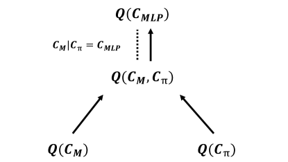
Dominance of Interpreting MLPs. We prove that when dealing with complexity classes of explainability queries that are from the polynomial hierarchy (such as NP, , etc.), the complexity class associated with the MLP always dominates the overall complexity. Hence, the exact complexity class of when and/or , is equivalent to that of . This claim holds for any class of polynomially computable functions.
Theorem 3.
Let be classes of polynomially computable functions such that or . If is -complete, where is a complexity class of the polynomial hierarchy (or the class associated with its counting problem), then is also -complete.
The “hardness” part of Theorem 3 is a direct consequence of Theorems 1 and 2. However, when specifically considering MLPs, completeness also holds. The proof of this claim is relegated to the appendix, and is a result of the fact that any Boolean circuit can be polynomially reduced to an MLP [12]. This relation implies that the “hardest” possible complexity class in the polynomial hierarchy is always associated with the one for interpreting an MLP over . Fig. 1 depicts the relations among different complexity classes, as derived from Theorems 1, 2, and 3.
In Table 1, we exemplify the aforementioned explainability queries (MCR, MSR, and CC) and a specific scenario where is set to either or , whereas the context indicator is set to (this is the case of our running example, in which the OOD detection is performed using a more expressive model than the original classifier). Hence, Theorem 3 implies that the complexity of solving the aligned query is primarily determined by the complexity involved in using an MLP, as summarized in Table 1.
| Q() | Q(, ) | Q() | Q(, ) | ||
|---|---|---|---|---|---|
| MCR | PTIME | NP-complete | PTIME | NP-complete | |
| MSR | NP-complete | -complete | PTIME | -complete | |
| CC | PTIME | #P-complete | #P-complete | #P-complete | |
5 “Self-Alignment”: Incorporating Social Alignment within a Single Model
Until now, we focused on the general scenario in which and are chosen from two different model classes (for instance is a decision tree, and is a neural network). However, in some cases, and can be two models of the same type, i.e., from the same class. In this scenario, given a classifier and an OOD detector, both from the same class, practitioners might decide to train a single model that learns both the prediction task and the alignment task. More formally, we say that a single model class is “self-aligned” when it is expressive enough to incorporate this dual procedure. This is demonstrated by the fact that given a model and a context indicator , a new model can be efficiently constructed to show the alignment of with respect to the distribution indicated by :
Definition 4.
A class of models is self-aligned if for any , and any inputs x and , there exists a polynomially constructible function , such that:
| (6) |
Intuitively, for any possible explainability query within (decision or counting), explanations of , aligned by , can be expressed by a single aggregated function . Clearly, must be at least as expressive as the original models and . This raises the question of how expressive a class of models should be, for it to be self-aligned.
Theorem 4.
Given a class of models , if for any , we can polynomially construct , for [op], then is self-aligned.
Intuitively, classes of models that are capable of expressing the logical operators and are capable of “capturing” that a given explanation form is determined by its underlying distribution. The proof of this theorem is relegated to the appendix, and can be obtained by showing an equivalence between the two underlying formalizations.
If self-alignment implies that, given a prediction model and a context indicator , we can attain a single aggregated model — then clearly the computational complexity of interpreting with respect to (i.e., the complexity of ) is correlated to the complexity of interpreting (i.e., the complexity of ). This can be demonstrated by the subsequent proposition:
Proposition 2.
If the conditions in Theorem 4 hold for a class of models , then .
Model-Specific Results
We move on to analyze which of the aforementioned model classes incorporate self-alignment. First, we show that both FBDDs and MLPs are self-aligned, which is a result of their capability to polynomially express and relations within their class:
Proposition 3.
FBDDs and MLPs are self-aligned, and hence, it follows that: and .
However, in contrast to decision trees and neural networks, linear classifiers lack the ability to capture the notion of self-alignment. It is important to note that a single Perceptron cannot inherently represent the and relations over two other Perceptrons. That said, it is worth emphasizing that this observation alone does not conclusively establish their lack of self-alignment, as this condition is sufficient but not necessary. To rigorously prove the inability of Perceptrons to be self-aligned, we prove the subsequent proposition:
Proposition 4.
While the query MCR can be solved in polynomial time, the query MCR is NP-complete.
Proof sketch. Membership results from the fact that we can guess a subset of features and validate whether it is contrastive for and whether it is also in-distribution (by feeding it to ). For hardness, we reduce from SSP (the k-subset-sum problem), which is a classic NP-complete problem. The reduction exploits the ranges of the Perceptrons of both and in order to bind the target sum of the subset, both from above and from below.
Building upon Proposition 4, we can deduce the following corollary (proved in the appendix):
Theorem 5.
Assuming that , the class is not self-aligned.
These findings underscore a crucial aspect concerning the interpretability of Perceptrons. While producing explanations pertaining to them can be achieved with low computational complexity (providing further evidence of their interpretability), they are not self-aligned. Consequently, obtaining aligned explanations using Perceptrons necessitates the adoption of a more sophisticated model, that is expressive enough to incorporate social alignment — and this, in turn, can significantly increase the overall complexity of their interpretation.
6 Related Work
This work continues a line of research that focuses on Formal XAI [46, 89, 9, 7, 48, 13, 14]. Prior studies have already investigated the explanation forms that were analyzed within our work [7, 89, 9, 7], including sufficiency-based explainability queries (MSR) [47, 69], contrastive/counterfactual-based queries (MCR) [81, 49], and counting-based queries (CC) [28]. Other work [36] defined formal notions of sufficient and contrastive reasons under specific contexts and suggested ways to compute them on a wide range of models [96]. However, these explanation forms were not analyzed with respect to their overarching computational complexity. Closer to ours is the work of Cooper et al. [21] which analyzes different properties (including the computational complexity) of sufficiency-based explanations under logical constraints. We also acknowledge the work of Arenas et al. [7], which describes a general logic-based explanation form, similar to our abstract query form. While their work focuses on explanations of first-order logic forms for decision queries, our approach is more expressive, encompassing second-order logic forms that incorporate both decision-based and counting-based explanations.
Another line of research examines the computational complexity of obtaining Shapley value-based explanations [8, 88, 72], where alignment with respect to a given distribution is vital [83]. Specifically, Van den Broeck et al. [88] identify a complexity gap in interpreting Shapley values when considering fully factorized or Naive Bayes-modeled distributions.
In some cases, the term “sufficient reason” is also defined as an abductive explanation [47] and correlates with the notion of a prime implicant for a Boolean classifier [28]. The CC query is associated with probabilistic notions of explainability, by correlating the precision of the explanation with the number of possible input completions [77, 89]. A similar notion, formally known as a -relevant set [52, 89], focuses on bounding this specific portion.
The dependency of explanations on OOD assignments has been studied extensively [97, 84, 33, 39, 59, 40, 95, 83]. Specifically, many heuristic-based tools and frameworks have been proposed for dealing with the OOD counterfactual problem in model explainability. These include marginalizing the prediction of the model over possible counterfactual assignments [100, 59, 95], sampling points in the proximity of the original input [20, 79, 77], as well as counterfactual training [38, 87] — a method that, similarly to adversarial training [99], seeks to robustify models to OOD counterfactuals. Other work focuses on mitigating the effect of OOD assignments on the computation of Shapley values [83, 56, 85]. In spite of these notable accomplishments, the theoretical analysis of the OOD counterfactual problem with respect to its computational complexity has yet to be thoroughly examined.
7 Conclusion
Computational complexity theory stands as a potential avenue to formally assess the interpretability of various ML models. Prior research examined this by considering two main factors: the model type and the explanation form. We claim that a third and important factor should be taken into consideration — the underlying distribution over which the explanation is computed. To achieve this goal, we generalize existing explainability queries and show how a unified form can describe the desired social alignment requirement for any explanation form under our second-order logic formalization. Moreover, we present a framework for assessing the computational complexity of these queries and demonstrate that, for a broad range of model types and query forms, providing socially aligned explanations is as hard as interpreting a model designed to detect OOD inputs. As OOD detection is known to be substantially difficult, such models may often require more expressive capacity than the original classification models, significantly impacting the overall complexity of model interpretation. Finally, we provide an analysis of the required capacity of models to inherently produce aligned explanations without using an external OOD detector. We hope that our work serves as a foundation for a deeper mathematical understanding of the interpretability pertaining to various ML models.
8 Limitations and Future Work
Our framework can be extended along several different axes. First and foremost, we note that assuming the existence of a context indicator for identifying OOD inputs is highly non-trivial. Previous work, both theoretical and practical, has highlighted the challenges associated with obtaining such an OOD detector [32, 73, 41, 80, 16]. However, it is important to emphasize that our framework does not necessarily assume the complete accuracy or correctness of such a classifier. Instead, can be viewed as a function that provides an approximation of the underlying context . Therefore, future research endeavors could center around evaluating the computational complexity of specific approximations tailored to particular contexts of interest. While these approximations may only offer a partially guaranteed solution to the alignment issue, they may still exhibit an improved complexity overall.
Other limitations correspond to similar (non-aligned) approaches for analyzing the computational complexity of obtaining explanations [12, 89, 15]. Firstly, our analysis considers only a worst-case scenario that may change under various parameter-specific configurations. Secondly, the natural subjectivity of interpretability makes it challenging to analyze the computational complexity of interpreting a model in a single “correct” way. To address this issue, theoretical frameworks define various explainability queries and evaluate them separately. We regard our proof for a wide range of explainability queries (the abstract query form) as potential evidence that the shared characteristics among different types of explainability queries can be utilized to offer more generalized assessments.
Finally, we highlight that our study primarily concentrates on an OOD detector , which classifies each input as either in-distribution or OOD, rather than on the input distribution itself. This approach is due to the strictly formal nature of the explanations we investigate; an explanation is either valid or not, necessitating a definitive categorization of the presence or absence of each input. In contrast, probabilistic explanation forms, such as -relevant sets [89, 52] or Shapley values [64, 83], are defined in relation to the distribution itself and can also be assessed based on the computational complexity of obtaining them. For instance, a recent study by Marzouk et al. [72] explores the computational complexity of calculating Shapley values within Markovian distributions. Future research can focus on expanding the strictly formal explanation framework discussed here to include probabilistic explanation forms as well, where complexity assessments would focus directly on the input distribution rather than on the OOD detector . Other, broader future work can explore the relation between the computational complexity of generating explanations (our current focus) and the complexity of the explanations themselves. This can be achieved using various tools, such as Kolmogorov complexity. We also cover additional extensions of our framework in the appendix.
Acknowledgments
This work was partially funded by the European Union (ERC, VeriDeL, 101112713). Views and opinions expressed are however those of the author(s) only and do not necessarily reflect those of the European Union or the European Research Council Executive Agency. Neither the European Union nor the granting authority can be held responsible for them. The work of Amir was further supported by a scholarship from the Clore Israel Foundation.
References
- Amir et al. [2021a] G. Amir, M. Schapira, and G. Katz. Towards Scalable Verification of Deep Reinforcement Learning. In Proc. 21st Int. Conf. on Formal Methods in Computer-Aided Design (FMCAD), pages 193–203, 2021a.
- Amir et al. [2021b] G. Amir, H. Wu, C. Barrett, and G. Katz. An SMT-Based Approach for Verifying Binarized Neural Networks. In Proc. 27th Int. Conf. on Tools and Algorithms for the Construction and Analysis of Systems (TACAS), pages 203–222, 2021b.
- Amir et al. [2022] G. Amir, T. Zelazny, G. Katz, and M. Schapira. Verification-Aided Deep Ensemble Selection. In Proc. 22nd Int. Conf. on Formal Methods in Computer-Aided Design (FMCAD), pages 27–37, 2022.
- Amir et al. [2023a] G. Amir, D. Corsi, R. Yerushalmi, L. Marzari, D. Harel, A. Farinelli, and G. Katz. Verifying Learning-Based Robotic Navigation Systems. In Proc. 29th Int. Conf. on Tools and Algorithms for the Construction and Analysis of Systems (TACAS), pages 607–627, 2023a.
- Amir et al. [2023b] G. Amir, Z. Freund, G. Katz, E. Mandelbaum, and I. Refaeli. veriFIRE: Verifying an Industrial, Learning-Based Wildfire Detection System. In Proc. 25th Int. Symposium on Formal Methods (FM), pages 648–656, 2023b.
- Amir et al. [2023c] G. Amir, O. Maayan, T. Zelazny, G. Katz, and M. Schapira. Verifying Generalization in Deep Learning. In Proc. 35th Int. Conf. on Computer Aided Verification (CAV), pages 438–455, 2023c.
- Arenas et al. [2021a] M. Arenas, D. Baez, P. Barceló, J. Pérez, and B. Subercaseaux. Foundations of Symbolic Languages for Model Interpretability. In Proc. 34th Int. Conf. on Advances in Neural Information Processing Systems (NeurIPS), pages 11690–11701, 2021a.
- Arenas et al. [2021b] M. Arenas, P. Barceló, L. Bertossi, and M. Monet. The Tractability of SHAP-Score-Based Explanations for Classification over Deterministic and Decomposable Boolean Circuits. In Proc. 35th AAAI Conf. on Artificial Intelligence, pages 6670–6678, 2021b.
- Arenas et al. [2022] M. Arenas, P. Barceló, M. Romero Orth, and B. Subercaseaux. On Computing Probabilistic Explanations for Decision Trees. In Proc. 35th Int. Conf. on Advances in Neural Information Processing Systems (NeurIPS), pages 28695–28707, 2022.
- Arora and Barak [2009] S. Arora and B. Barak. Computational Complexity: A Modern Approach. Cambridge University Press, 2009.
- Audemard et al. [2023] G. Audemard, J. Lagniez, P. Marquis, and N. Szczepanski. Computing Abductive Explanations for Boosted Trees. In Proc. 26th Int. Conf. on Artificial Intelligence and Statistics (AISTATS), 2023.
- Barceló et al. [2020] P. Barceló, M. Monet, J. Pérez, and B. Subercaseaux. Model Interpretability through the Lens of Computational Complexity. In Proc. 33rd Int. Conf. on Advances in Neural Information Processing Systems (NeurIPS), pages 15487–15498, 2020.
- Bassan and Katz [2023] S. Bassan and G. Katz. Towards Formal Approximated Minimal Explanations of Neural Networks. In Proc. 29th Int. Conf. on Tools and Algorithms for the Construction and Analysis of Systems (TACAS), pages 187–207, 2023.
- Bassan et al. [2023] S. Bassan, G. Amir, D. Corsi, I. Refaeli, and G. Katz. Formally Explaining Neural Networks within Reactive Systems. In Proc. 23rd Int. Conf. on Formal Methods in Computer-Aided Design (FMCAD), pages 10–22, 2023.
- Bassan et al. [2024] S. Bassan, G. Amir, and G. Katz. Local vs. Global Interpretability: A Computational Complexity Perspective. In Proc. 41st Int. Conf. on Machine Learning (ICML), 2024.
- Berend et al. [2020] D. Berend, X. Xie, L. Ma, L. Zhou, Y. Liu, C. Xu, and J. Zhao. Cats are not Fish: Deep Learning Testing Calls for Out-of-Distribution Awareness. In Proc. 35th IEEE/ACM Int. Conf. on Automated Software Engineering (ASE), pages 1041–1052, 2020.
- Boumazouza et al. [2021] R. Boumazouza, F. Cheikh-Alili, B. Mazure, and K. Tabia. ASTERYX: A Model-Agnostic SAT-Based Approach for Symbolic and Score-Based Explanations. In Proc. 30th ACM Int. Conf. on Information & Knowledge Management (CIKM), pages 120–129, 2021.
- Bunel et al. [2018] R. Bunel, I. Turkaslan, P. Torr, P. Kohli, and P. Mudigonda. A Unified View of Piecewise Linear Neural Network Verification. In Proc. 32nd Conf. on Neural Information Processing Systems (NeurIPS), pages 4795–4804, 2018.
- Casadio et al. [2022] M. Casadio, E. Komendantskaya, M. Daggitt, W. Kokke, G. Katz, G. Amir, and I. Refaeli. Neural Network Robustness as a Verification Property: A Principled Case Study. In Proc. 34th Int. Conf. on Computer Aided Verification (CAV), pages 219–231, 2022.
- Chang et al. [2019] C. Chang, E. Creager, A. Goldenberg, and D. Duvenaud. Explaining Image Classifiers by Counterfactual Generation. In Proc. 7th Int. Conf. on Learning Representations (ICLR), 2019.
- Cooper and Amgoud [2023] M. Cooper and L. Amgoud. Abductive Explanations of Classifiers under Constraints: Complexity and Properties. In 26th European Conf. on Artificial Intelligence (ECAI), 2023.
- Corsi et al. [2022] D. Corsi, R. Yerushalmi, G. Amir, A. Farinelli, D. Harel, and G. Katz. Constrained Reinforcement Learning for Robotics via Scenario-Based Programming, 2022. Technical Report. https://arxiv.org/abs/2206.09603.
- Corsi et al. [2024a] D. Corsi, G. Amir, G. Katz, and A. Farinelli. Analyzing Adversarial Inputs in Deep Reinforcement Learning, 2024a. Technical Report. https://arxiv.org/abs/2402.05284.
- Corsi et al. [2024b] D. Corsi, G. Amir, A. Rodríguez, C. Sánchez, G. Katz, and R. Fox. Verification-Guided Shielding for Deep Reinforcement Learning. In Proc. 1st Int. Reinforcement Learning Conf. (RLC), 2024b.
- Darwiche and Hirth [2020] A. Darwiche and A. Hirth. On the Reasons Behind Decisions. In Proc. 23rd European Conf. on Artificial Intelligence (ECAI), pages 712–720, 2020.
- Darwiche and Hirth [2023] A. Darwiche and A. Hirth. On the (Complete) Reasons Behind Decisions. Journal of Logic, Language and Information, 32(1):63–88, 2023.
- Darwiche and Ji [2022] A. Darwiche and C. Ji. On the Computation of Necessary and Sufficient Explanations. In Proc. 36th AAAI Conf. on Artificial Intelligence, pages 5582–5591, 2022.
- Darwiche and Marquis [2002] A. Darwiche and P. Marquis. A Knowledge Compilation Map. Journal of Artificial Intelligence Research (JAIR), 17:229–264, 2002.
- Ehlers [2017] R. Ehlers. Formal Verification of Piece-Wise Linear Feed-Forward Neural Networks. In Proc. 15th Int. Symp. on Automated Technology for Verification and Analysis (ATVA), pages 269–286, 2017.
- Elboher et al. [2020] Y. Elboher, J. Gottschlich, and G. Katz. An Abstraction-Based Framework for Neural Network Verification. In Proc. 32nd Int. Conf. on Computer Aided Verification (CAV), pages 43–65, 2020.
- Fagin [1974] R. Fagin. Generalized First-Order Spectra and Polynomial-Time Recognizable Sets. Complexity of Computation, 7:43–73, 1974.
- Fang et al. [2022] Z. Fang, Y. Li, J. Lu, J. Dong, B. Han, and F. Liu. Is Out-of-Distribution Detection Learnable? In Proc. 36th Int. Conf. on Advances in Neural Information Processing Systems (NeurIPS), 2022.
- Fong and Vedaldi [2017] R. Fong and A. Vedaldi. Interpretable Explanations of Black Boxes by Meaningful Perturbation. In Proc. IEEE Int. Conf. on Computer Vision (ICCV), pages 3429–3437, 2017.
- Gardner and Dorling [1998] M. Gardner and S. Dorling. Artificial Neural Networks (the Multilayer Perceptron)— a Review of Applications in the Atmospheric Sciences. Atmospheric Environment, 32(14-15):2627–2636, 1998.
- Gehr et al. [2018] T. Gehr, M. Mirman, D. Drachsler-Cohen, E. Tsankov, S. Chaudhuri, and M. Vechev. AI2: Safety and Robustness Certification of Neural Networks with Abstract Interpretation. In Proc. 39th IEEE Symposium on Security and Privacy (S&P), 2018.
- Gorji and Rubin [2022] N. Gorji and S. Rubin. Sufficient Reasons for Classifier Decisions in the Presence of Domain Constraints. In Proc. 36th AAAI Conf. on Artificial Intelligence, pages 5660–5667, 2022.
- Halpern and Pearl [2005] J. Halpern and J. Pearl. Causes and Explanations: A Structural-Model Approach. Part I: Causes. The British Journal for the Philosophy of Science, 2005.
- Hase et al. [2021] P. Hase, H. Xie, and M. Bansal. The Out-of-Distribution Problem in Explainability and Search Methods for Feature Importance Explanations. In Proc. 34th Int. Conf. on Advances in Neural Information Processing Systems (NeurIPS), pages 3650–3666, 2021.
- Hooker et al. [2019] S. Hooker, D. Erhan, P. Kindermans, and B. Kim. A Benchmark for Interpretability Methods in Deep Neural Networks. In Proc. 32nd Int. Conf. on Advances in Neural Information Processing Systems (NeurIPS), 2019.
- Hsieh et al. [2021] C. Hsieh, C. Yeh, X. Liu, P. Ravikumar, S. Kim, S. Kumar, and C. Hsieh. Evaluations and Methods for Explanation through Robustness Analysis. In Proc. 9th Int. Conf. on Learning Representations (ICLR), 2021.
- Hsu et al. [2020] Y. Hsu, Y. Shen, H. Jin, and Z. Kira. Generalized ODIN: Detecting Out-of-Distribution Image Without Learning From Out-of-Distribution Data. In Proc. IEEE/CVF Conf. on Computer Vision and Pattern Recognition (CVPR), 2020.
- Huang and Marques-Silva [2023] X. Huang and J. Marques-Silva. From Robustness to Explainability and Back Again, 2023. Technical Report. https://arxiv.org/abs/2306.03048.
- Huang et al. [2020] X. Huang, D. Kroening, W. Ruan, J. Sharp, Y. Sun, E. Thamo, M. Wu, and X. Yi. A Survey of Safety and Trustworthiness of Deep Neural Networks: Verification, Testing, Adversarial attack and Defence, and Interpretability. Computer Science Review, 37:100270, 2020.
- Huang et al. [2021] X. Huang, Y. Izza, A. Ignatiev, and J. Marques-Silva. On Efficiently Explaining Graph-Based Classifiers, 2021. Technical Report. https://arxiv.org/abs/2106.01350.
- Huang et al. [2023] X. Huang, M. Cooper, A. Morgado, J. Planes, and J. Marques-Silva. Feature Necessity & Relevancy in ML Classifier Explanations. In Proc. 29th Int. Conf. on Tools and Algorithms for the Construction and Analysis of Systems (TACAS), pages 167–186, 2023.
- Ignatiev [2020] A. Ignatiev. Towards Trustable Explainable AI. In Proc. 29th Int. Joint Conf. on Artificial Intelligence (IJCAI), pages 5154–5158, 2020.
- Ignatiev et al. [2019a] A. Ignatiev, N. Narodytska, and J. Marques-Silva. Abduction-Based Explanations for Machine Learning Models. In Proc. 33rd AAAI Conf. on Artificial Intelligence, pages 1511–1519, 2019a.
- Ignatiev et al. [2019b] A. Ignatiev, N. Narodytska, and J. Marques-Silva. On Relating Explanations and Adversarial Examples. In Proc. 32nd Int. Conf. on Advances in Neural Information Processing Systems (NeurIPS), 2019b.
- Ignatiev et al. [2020] A. Ignatiev, N. Narodytska, N. Asher, and J. Marques-Silva. From Contrastive to Abductive Explanations and Back Again. In Proc. Int. Conf. Italian Association for Artificial Intelligence, 2020.
- Ignatiev et al. [2022] A. Ignatiev, Y. Izza, P. Stuckey, and J. Marques-Silva. Using MaxSAT for Efficient Explanations of Tree Ensembles. In Proc. 36th AAAI Conf. on Artificial Intelligence, pages 3776–3785, 2022.
- Izza and Marques-Silva [2021] Y. Izza and J. Marques-Silva. On Explaining Random Forests with SAT. In Proc. 30th Int. Joint Conf. on Artificial Intelligence (IJCAI), 2021.
- Izza et al. [2021] Y. Izza, A. Ignatiev, N. Narodytska, M. Cooper, and J. Marques-Silva. Efficient Explanations with Relevant Sets, 2021. Technical Report. https://arxiv.org/abs/2106.00546.
- Izza et al. [2022] Y. Izza, A. Ignatiev, and J. Marques-Silva. On Tackling Explanation Redundancy in Decision Trees. Journal of Artificial Intelligence Research (JAIR), 75:261–321, 2022.
- Izza et al. [2024] Y. Izza, X. Huang, A. Morgado, J. Planes, A. Ignatiev, and J. Marques-Silva. Distance-Restricted Explanations: Theoretical Underpinnings & Efficient Implementation, 2024. Technical Report. https://arxiv.org/abs/2405.08297.
- Jacoby et al. [2020] Y. Jacoby, C. Barrett, and G. Katz. Verifying Recurrent Neural Networks using Invariant Inference. In Proc. 18th Int. Symposium on Automated Technology for Verification and Analysis (ATVA), pages 57–74, 2020.
- Janzing et al. [2020] D. Janzing, L. Minorics, and P. Blöbaum. Feature Relevance Quantification in Explainable AI: A Causal Problem. In Proc. 23rd Int. Conf. on Artificial Intelligence and Statistics (AISTATS), pages 2907–2916, 2020.
- Katz et al. [2017] G. Katz, C. Barrett, D. Dill, K. Julian, and M. Kochenderfer. Reluplex: An Efficient SMT Solver for Verifying Deep Neural Networks. In Proc. 29th Int. Conf. on Computer Aided Verification (CAV), pages 97–117, 2017.
- Katz et al. [2019] G. Katz, D. Huang, D. Ibeling, K. Julian, C. Lazarus, R. Lim, P. Shah, S. Thakoor, H. Wu, A. Zeljić, D. Dill, M. Kochenderfer, and C. Barrett. The Marabou Framework for Verification and Analysis of Deep Neural Networks. In Proc. 31st Int. Conf. on Computer Aided Verification (CAV), pages 443–452, 2019.
- Kim et al. [2020] S. Kim, J. Yi, E. Kim, and S. Yoon. Interpretation of NLP Models Through Input Marginalization. In Proc. Conf. on Empirical Methods in Natural Language Processing (EMNLP), 2020.
- Könighofer et al. [2020] B. Könighofer, F. Lorber, N. Jansen, and R. Bloem. Shield Synthesis for Reinforcement Learning. In Proc. Int. Symposium on Leveraging Applications of Formal Methods, Verification and Validation (ISoLA), pages 290–306, 2020.
- La Malfa et al. [2021] E. La Malfa, A. Zbrzezny, R. Michelmore, N. Paoletti, and M. Kwiatkowska. On Guaranteed Optimal Robust Explanations for NLP Models. In Proc. 30th Int. Joint Conf. on Artificial Intelligence (IJCAI), 2021.
- Lee [1959] C. Lee. Representation of Switching Circuits by Binary-Decision Programs. The Bell System Technical Journal, 38(4):985–999, 1959.
- Liang et al. [2021] C. Liang, P. Huang, W. Lai, and Z. Ruan. GAN-Based Out-of-Domain Detection Using Both In-Domain and Out-of-Domain Samples. In Proc. IEEE Int. Conf. on Acoustics, Speech and Signal Processing (ICASSP), pages 7663–7667, 2021.
- Lundberg and Lee [2017] S. Lundberg and S. Lee. A Unified Approach to Interpreting Model Predictions. In Proc. 30th Int. Conf. on Advances in Neural Information Processing Systems (NeurIPS), 2017.
- Lyu et al. [2020] Z. Lyu, C. Ko, Z. Kong, N. Wong, D. Lin, and L. Daniel. Fastened Crown: Tightened Neural Network Robustness Certificates. In Proc. 34th AAAI Conf. on Artificial Intelligence (AAAI), pages 5037–5044, 2020.
- Mandal et al. [2024a] U. Mandal, G. Amir, H. Wu, I. Daukantas, F. Newell, U. Ravaioli, B. Meng, M. Durling, M. Ganai, T. Shim, G. Katz, and C. Barrett. Formally Verifying Deep Reinforcement Learning Controllers with Lyapunov Barrier Certificates. In Proc. 24th Int. Conf. on Formal Methods in Computer-Aided Design (FMCAD), 2024a.
- Mandal et al. [2024b] U. Mandal, G. Amir, H. Wu, I. Daukantas, F. Newell, U. Ravaioli, B. Meng, M. Durling, K. Hobbs, M. Ganai, T. Shim, G. Katz, and C. Barrett. Safe and Reliable Training of Learning-Based Aerospace Controllers. In Proc. 43rd Digital Avionics Systems Conf. (DASC), 2024b.
- Marques-Silva and Ignatiev [2022] J. Marques-Silva and A. Ignatiev. Delivering Trustworthy AI through formal XAI. In Proc. 36th AAAI Conf. on Artificial Intelligence, pages 3806–3814, 2022.
- Marques-Silva et al. [2020] J. Marques-Silva, T. Gerspacher, M. Cooper, A. Ignatiev, and N. Narodytska. Explaining Naive Bayes and Other Linear Classifiers with Polynomial Time and Delay. In Proc. 33rd Int. Conf. on Advances in Neural Information Processing Systems (NeurIPS), pages 20590–20600, 2020.
- Marques-Silva et al. [2021] J. Marques-Silva, T. Gerspacher, M. Cooper, A. Ignatiev, and N. Narodytska. Explanations for Monotonic Classifiers. In Proc. 38th Int. Conf. on Machine Learning (ICML), 2021.
- Marzari et al. [2023] L. Marzari, D. Corsi, F. Cicalese, and A. Farinelli. The #DNN-Verification problem: Counting Unsafe Inputs for Deep Neural Networks. In Proc. 32nd Int. Joint Conf. on Artificial Intelligence (IJCAI), 2023.
- Marzouk and de La Higuera [2024] R. Marzouk and C. de La Higuera. On the Tractability of SHAP Explanations under Markovian Distributions, 2024. Technical Report. http://arxiv.org/abs/2405.02936.
- Morteza and Li [2022] P. Morteza and Y. Li. Provable Guarantees for Understanding Out-of-Distribution Detection. In Proc. 36th AAAI Conf. on Artificial Intelligence, pages 7831–7840, 2022.
- Poyiadzi et al. [2020] R. Poyiadzi, K. Sokol, R. Santos-Rodriguez, T. De Bie, and P. Flach. FACE: Feasible and Actionable Counterfactual Explanations. In Proc. AAAI/ACM Conf. on AI, Ethics, and Society (AIES), 2020.
- Ralston et al. [2003] A. Ralston, E. Reilly, and D. Hemmendinger. Encyclopedia of Computer Science. John Wiley and Sons Ltd., 2003.
- Ramchoun et al. [2016] H. Ramchoun, Y. Ghanou, M. Ettaouil, and M. Amine Janati Idrissi. Multilayer Perceptron: Architecture Optimization and Training. Int. Journal of Interactive Multimedia and Artificial Intelligence, 2016.
- Ribeiro et al. [2018] M. Ribeiro, S. Singh, and C. Guestrin. Anchors: High-Precision Model-Agnostic Explanations. In Proc. 32nd AAAI Conf. on Artificial Intelligence, 2018.
- Rodriguez et al. [2024] A. Rodriguez, G. Amir, D. Corsi, C. Sanchez, and G. Katz. Shield Synthesis for LTL Modulo Theories , 2024. Technical Report. https://arxiv.org/abs/2406.04184.
- Sanyal and Ren [2021] S. Sanyal and X. Ren. Discretized Integrated Gradients for Explaining Language Models. In Proc. Conf. on Empirical Methods in Natural Language Processing (EMNLP), 2021.
- Serrà et al. [2019] J. Serrà, D. Álvarez, V. Gómez, O. Slizovskaia, J. Núñez, and J. Luque. Input Complexity and Out-of-Distribution Detection with Likelihood-Based Generative Models. In Proc. 7th Int. Conf. on Learning Representations (ICLR), 2019.
- Shih et al. [2018] A. Shih, A. Choi, and A. Darwiche. Formal Verification of Bayesian Network Classifiers. In Proc. Int. Conf. on Probabilistic Graphical Models (PGM), pages 427–438, 2018.
- Sun et al. [2019] X. Sun, H. Khedr, and Y. Shoukry. Formal Verification of Neural Network Controlled Autonomous Systems. In Proc. 22nd ACM Int. Conf. on Hybrid Systems: Computation and Control (HSCC), 2019.
- Sundararajan and Najmi [2020] M. Sundararajan and A. Najmi. The Many Shapley Values for Model Explanation. In Proc. 37th Int. Conf. on Machine Learning (ICML), pages 9269–9278, 2020.
- Sundararajan et al. [2017] M. Sundararajan, A. Taly, and Q. Yan. Axiomatic Attribution for Deep Networks. In Proc. 34th Int. Conf. on Machine Learning (ICML), 2017.
- Taufiq et al. [2023] M. Taufiq, P. Blöbaum, and L. Minorics. Manifold Restricted Interventional Shapley Values. In Proc. 26th Int. Conf. on Artificial Intelligence and Statistics (AISTATS), 2023.
- Tran et al. [2020] H. Tran, S. Bak, and T. Johnson. Verification of Deep Convolutional Neural Networks Using ImageStars. In Proc. 32nd Int. Conf. on Computer Aided Verification (CAV), pages 18–42, 2020.
- Vafa et al. [2021] K. Vafa, Y. Deng, D. Blei, and A. Rush. Rationales for Sequential Predictions. In Proc. Conf. on Empirical Methods in Natural Language Processing (EMNLP), 2021.
- Van den Broeck et al. [2022] G. Van den Broeck, A. Lykov, M. Schleich, and D. Suciu. On the Tractability of SHAP Explanations. Journal of Artificial Intelligence Research (JAIR), 74:851–886, 2022.
- Wäldchen et al. [2021] S. Wäldchen, J. Macdonald, S. Hauch, and G. Kutyniok. The Computational Complexity of Uderstanding Binary Classifier Decisions. Journal of Artificial Intelligence Research (JAIR), 70:351–387, 2021.
- Wu et al. [2024a] H. Wu, O. Isac, A. Zeljić, T. Tagomori, M. Daggitt, W. Kokke, I. Refaeli, G. Amir, K. Julian, S. Bassan, P. Huang, O. Lahav, M. Wu, M. Zhang, E. Komendantskaya, G. Katz, and C. Barrett. Marabou 2.0: A Versatile Formal Analyzer of Neural Networks. In Proc. 36th Int. Conf. on Computer Aided Verification (CAV), 2024a.
- Wu et al. [2024b] M. Wu, H. Wu, and C. Barrett. Verix: Towards Verified Explainability of Deep Neural Networks. In Proc. 36th Int. Conf. on Advances in Neural Information Processing Systems (NeurIPS), 2024b.
- Xuan et al. [2022] X. Xuan, P. Xizhou, L. Nan, H. Xing, M. Lin, Z. Xiaoguang, and D. Ning. GAN-Based Anomaly Detection: A Review. Neurocomputing, 493, 2022.
- Yerushalmi et al. [2022] R. Yerushalmi, G. Amir, A. Elyasaf, D. Harel, G. Katz, and A. Marron. Scenario-Assisted Deep Reinforcement Learning. In Proc. 10th Int. Conf. on Model-Driven Engineering and Software Development (MODELSWARD), pages 310–319, 2022.
- Yerushalmi et al. [2023] R. Yerushalmi, G. Amir, A. Elyasaf, D. Harel, G. Katz, and A. Marron. Enhancing Deep Reinforcement Learning with Scenario-Based Modeling. SN Computer Science, 4(2):156, 2023.
- Yi et al. [2020] J. Yi, E. Kim, S. Kim, and S. Yoon. Information-Theoretic Visual Explanation for Black-Box Classifiers, 2020. Technical Report. https://arxiv.org/abs/2009.11150.
- Yu et al. [2022] J. Yu, A. Ignatiev, P. Stuckey, N. Narodytska, and J. Marques-Silva. Eliminating The Impossible, Whatever Remains Must Be True, 2022. Technical Report. https://arxiv.org/abs/2206.09551.
- Zaidan et al. [2007] O. Zaidan, J. Eisner, and C. Piatko. Using “Annotator Rationales” to Improve Machine Learning for Text Categorization. In Proc. Conf. North American Chapter of the Association for Computational Linguistics (NAACL), pages 260–267, 2007.
- Zhang et al. [2020] H. Zhang, M. Shinn, A. Gupta, A. Gurfinkel, N. Le, and N. Narodytska. Verification of Recurrent Neural Networks for Cognitive Tasks via Reachability Analysis. In Proc. 24th European Conf. on Artificial Intelligence (ECAI), pages 1690–1697, 2020.
- Zhao et al. [2022] W. Zhao, S. Alwidian, and Q. Mahmoud. Adversarial Training Methods for Deep Learning: A Systematic Review. Algorithms, 15(8):283, 2022.
- Zintgraf et al. [2017] L. Zintgraf, T. Cohen, T. Adel, and M. Welling. Visualizing Deep Neural Network Decisions: Prediction Difference Analysis. In Proc. 7th Int. Conf. on Learning Representations (ICLR), 2017.
Appendix
The appendix contains definitions, formalizations, and proofs that were mentioned throughout the paper:
-
Appendix A describes the abstract query form.
-
Appendix B describes the specific model types, and the universal model properties.
-
Appendix C contains an analysis of the model-specific properties.
-
Appendix D includes the proofs for the theorems and propositions mentioned in the paper.
-
Appendix E includes possible extensions of our theoretical framework.
Appendix A Abstract Query Form
We present a comprehensive analysis of the abstract query form discussed in our paper, providing a more detailed explanation of our process.
The Misaligned Case
Initially, we introduce the query form for the “misaligned” case, referring to the abstract query form that does not consider the context indicator as an input. We formulate this specific scenario and demonstrate its applicability in generalizing the various discussed explainability queries: MSR, CC, and MCR, all in their misaligned versions. Subsequently, we proceed to outline the consequential query for the aligned scenario, where is taken into account, dismantling the effect of any OOD counterfactual. We then reiterate how the explainability queries of MSR, CC, and MCR, when considered in their aligned forms, are all specific instances of the abstract query .
Let denote the following conjunct:
| (7) |
Let denote an SOL formula that includes , where the variable is exclusively present in . In other words, is not found in any other conjunct of apart from . We denote the (misaligned) version of as any explainability query that takes , , and as inputs, where represents a set of additional arbitrary inputs. The output of is a satisfying solution to or the counting of . We are now able to formulate the abstract (misaligned) query form :
(Misaligned) (Abstract Query Form): Input: Model , input x, and input . Output: a Yes or No answer, to whether holds, or the number of assignments of .
It is important to highlight that the values of and z are implicitly present in . These values can either be included as part of the input , or they can be explicitly defined within . Now, we demonstrate how the aforementioned explainability queries (in their misaligned form) can be precisely formulated as specific instances of . We start by illustrating this for the relatively simpler scenarios of MCR and CC:
(Misaligned) MCR (Minimum Change Required): Input: Model , input x, and input . Output: Yes, if is satisfiable, and No otherwise.
(Misaligned) CC (Count Completions): Input: Model , input x, and input . Output: The number of assignments of .
Once again, it is worth noting that in these particular scenarios, the value of is derived from a subset of the input for the CC query, while for MCR, it is defined within . Now, we proceed to demonstrate how the sufficiency-based explainability query (MSR) can also be acquired. In this case, corresponds to the negation of :
(Misaligned) MSR (Minimum Sufficient Reason): Input: Model , input x, and input . Output: Yes, if is satisfiable, and No otherwise.
It is straightforward to show that this formalization of MSR is equivalent to its predefined versions, since:
| (8) | |||
In other words, a subset is sufficient to determine a prediction if and only if there does not exist any assignment to the complementary that is contrastive. This leads us to the fact that there exists a sufficient reason of size if and only if there exists some subset of size such that no possible assignment to is contrastive.
We note that when evaluating the complexity of the misaligned abstract explainability query , we consider it in relation to a single class of models. For instance, describes the complexity of obtaining a (misaligned) explainability query for a model using the (misaligned) abstract query form . Unlike the aligned version, we do not input two families of functions since the context indicator is not included as part of the input for these queries.
The Aligned Case
We now proceed to describe the aligned version of the abstract query form. In this case, we aim to construct a similar abstract query form with the additional requirement of neutralizing the influence of any OOD counterfactuals. This is obtained by adding an additional constraint, namely . To formally define this, we introduce as follows:
| (9) |
Similarly, we define as any SOL formula that includes , where and are exclusively included within . In other words, and are not present in any conjunct of except for . We denote the (aligned) version of as an explainability query that takes , , , and as inputs, where represents an arbitrary set of additional inputs. The output of is a solution (either decision or counting), over . Therefore, the abstract query form, in this case, can be expressed as follows:
(Abstract Query Form): Input:Model , input x, context indicator , and input . Output: a Yes or No answer, to whether holds, or the number of assignments of .
We briefly illustrate how this abstract query form encompasses all the previously defined explainability queries, including the aligned versions of MSR, MCR, and CC. Once again, it is straightforward to show that MCR and CC are instances of this abstract query form (this time, in the aligned version):
MCR (Minimum Change Required): Input: Model , input x, context indicator , and input . Output: Yes, if is satisfiable, and No otherwise.
CC (Count Completions): Input: Model , input x, context indicator , and input . Output: The number of assignments of .
Similarly to the misaligned case, the aligned version of the sufficiency-based query (MSR) can be obtained as follows:
MSR (Minimum Sufficient Reason): Input: Model , input x, context indicator , and input . Output: Yes, if is satisfiable, and No otherwise.
The equivalence between these specific instances and the predefined explainability queries holds in these particular scenarios. This is due to the following:
| (10) | |||
Recall that in the case of the aligned version of , the underlying computational complexity is evaluated by considering two classes of models: for the classification model and for the context indicator. For instance, represents the computational complexity of obtaining an explainability query for models with respect to the context indicators and an abstract query form .
Appendix B Model Types and Universal Properties
Model Types
Next, we provide a full description of the models that are taken into account within our work.
Binary Decision Diagram (BDD). A BDD [62] is a graphical representation of a Boolean function , realized by a directed, acyclic graph, for which: (i) each internal node (i.e., non-sink nodes) corresponds to a single feature ; (ii) each internal node has precisely two output edges, representing the values assigned to ; (iii) each leaf corresponds to either a true, or false, label; and (iv) each variable appears at most once, along any given path within the BDD.
Hence, every path from the root node to a leaf, corresponds to a specific input assignment , with matching the value of the leaf of the relevant path . Following previous conventions [12, 44, 45, 9], we regard the size of the BDD to be the total number of edges. We focus on the popular hypothesis class of “Free BDDs” (FBDDs), in which different paths may have various orderings of the input variables .
Multi-Layer Perceptron (MLP). Given a set of weight matrices , bias vectors and activation functions , a Multi-Layer Perceptron (MLP) [34, 76] , with hidden layers ( for ) and a single output layer (), is recursively defined based on the following series of functions:
| (11) |
outputs the value of the function , and corresponds to the input of the model. The weight matrices and biases are defined by a series of positive values representing the dimensions of their inputs. In addition, we assume that all the weights and biases (learned during training) have rational values, i.e., and . Notice that due to our focus on binary classifiers over , then it holds that: and . Furthermore, we consider the popular activation function. The last activation of MLPs is typically a sigmoid function, but since we are only interested in post-hoc interpretations, we can equivalently, without loss of generality, consider the last activation to correspond to the step function:
| (12) |
Perceptron. A Perceptron [75] is an MLP with a single layer (i.e., ): , for and . Hence, without loss of generality, for a Perceptron it holds that:
| (13) |
Universal Properties
Next, we provide the precise formalization for the universal properties over and that were mentioned within our study. These are that is symmetrically constructible, whereas is naively construcatble.
Definition 1.
A class of functions is symmetrically constructible if given a model , then can be constructed in polynomial time.
Definition 2.
A class of functions is naively constructible if for any value , then can be constructed in polynomial time.
Appendix C Model-Specific Properties
As mentioned above, our propositions and theorems are based on the universal properties formulated in Section B of the appendix. These qualities include symmetric constructability and naive constructability. In this section, we illustrate how these properties indeed hold for the particular models discussed in our work, namely FBDDs, Perceptrons, and MLPs. We emphasize that these are only particular illustrations, and that these properties can be proven to hold for a broader range of hypothesis classes. First, we recall Proposition 1:
Proposition 1.
FBDDs, Perceptrons, and MLPs are all symmetrically constructible and naively constructible.
To this end, we prove the following lemmas.
Lemma 1.
The class is naively constructible and symmetrically constructible.
It is straightforward to show this in the following manner: (i) given an FBDD we can construct by duplicating and negating all leaf nodes in the duplicated diagram; and (ii) given an input we can simply construct an FBDD with a single accepting path matching the assignment of x.
Lemma 2.
The class is naively constructible and symmetrically constructible.
MLPs can also be constructed symmetrically and naively in a straightforward manner. First, we state that for every MLP , we can construct, in linear time, an equivalent MLP , such that the weights and biases are integers (this can be achieved by multiplying the values by the lowest common denominator, as done in [12]). Next, for the bias in the last layer, we also add . This procedure guarantees that: (i) for every input , it holds that , i.e., the new MLP is equivalent to ; and (ii) there is no binary input such that for it holds that , i.e., no input is exactly on the decision boundary of (as all linear combinations of integers — remain integers, and the single bias is not an integer). Next, symmetric constructability for (and hence, for ) is acquired as follows. We can construct by negating the weights of the last layer (setting for all ) and negating the bias of the output layer . Since the last layer contains a single step function, negating the corresponding weights (and bias) will result in a flipped classification.
To show naive constructability, we make use of the following Lemma [12]:
Lemma 3.
Given a Boolean circuit , we can construct, in polynomial time, an MLP , which induces an equivalent Boolean function relative to .
Hence, as a direct corollary, it is possible to polynomially construct an MLP that corresponds to the Boolean circuit representing: .
Lemma 4.
The class is naively constructible and symmetrically constructible.
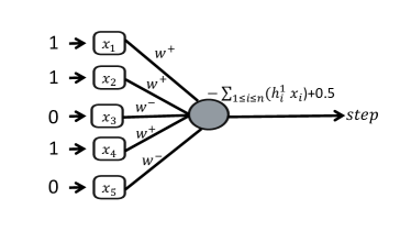
The symmetric construction proved for MLPs also holds directly for Perceptrons (by negating the weights of as well as the bias ). Given an input , naive constructability can be achieved by constructing a model where the corresponding single hidden layer is weighted such that for and for , for some user-defined value . The single bias term is set to . The intuition behind this construction is that it maximizes the contribution of the particular input x while rendering negative values for any other input in . An illustration of this construction is provided in Fig. 2. Also, we observe that this construction clearly serves as valid proof for the naive constructability of MLPs, but this was already trivially derived from the properties discussed in the previous section.
Appendix D Main Theorem Proofs
In this section, we prove all the theorems and propositions presented in the main text.
The Complexity of Obtaining Socially Aligned Explanations
First, we provide the proofs for Theorems 1 and 2, as discussed in the main text. More specifically:
Theorem 1.
If then .
Proof.
The proof is straightforward since given some the reduction can simply encode and return . Clearly, it holds that: , which concludes the correctness of the reduction. ∎
Theorem 2.
If is symmetrically constructible and is naively constructible, then .
Given some : the reduction checks whether is a valid encoding of a function in . If not, it returns an invalid encoding. If so, it constructs the negation function (based on our assumptions, this can be computed in polynomial time). Then, the reduction computes and constructs (also in polynomial time). If , the reduction returns , and if , it returns .
Let denote the SOL formula that corresponds to the solution of and let denote the SOL formula that corresponds to the solution of . Let us denote as the aforementioned conjunct (see Sec. A of the appendix) that corresponds to , and by the conjunct that corresponds to .
Assume . Since in this case it holds that , then:
For it holds that:
Assume that . In this case, the reduction sets to , and thus:
Where the last encoded conjunct is a tautology under this scenario. Overall, we get that:
This means that and are equivalent and hence any solution for SOL or #SOL will be equivalent to and . Thus, .
Assume that . In this case, the reduction sets to and thus:
Overall, we again obtain that:
Hence, again it holds that and are equivalent, and from the same reason stated above, it thus holds that .
Now, assume . In this case, the reduction initially checks the validity of the encoding, which includes that of . Hence, we are only left to check the cases where but . This implies that the SOL was unsatisfiable or, if is a counting query, that #SOL returned an incorrect count. Since the previous result demonstrated that and are equivalent under the assumption that , any assignment to will hold if and only if it holds to . Consequently, we can conclude that .
Theorem 3.
Let be classes of polynomially computable functions such that or . If is -complete, where is a complexity class of the polynomial hierarchy (or its associated counting class), then is also -complete.
Proof. The complexity classes within the polynomial hierarchy consist of the classes and for all . The class is defined as all languages such that there exists a polynomial time Turing machine and polynomials such that:
| (14) | |||
On the other hand, is defined respectively by alternating quantifiers , and hence . In the context of SOL, we define as a formula of the form:
| (15) |
where is a quantifier-free FOL formula over . Extending Fagin’s theorem [31] shows that a solution to an SOL formula with alternating quantifiers (starting with ) is -complete. We note that this holds in the case of finite structures, which is our setting, as for any we have a finite number of inputs. Since any SOL formula can be written as an SOL formula consisting of alternating quantifiers or , then by extending Fagin’s theorem [31], we can conclude that each SOL formula is associated with a class in the polynomial hierarchy (this holds in the case of finite structures, which is indeed our case, as we focus on discrete inputs). For example is -complete and is -complete (again, as in our case the formula includes models that are restricted to finite inputs). We note that for the counting case, each one of these complexity classes has a corresponding associated counting class, for example, the number of satisfying assignments for or .
Recall that each query is associated with an SOL formula and each aligned query is associated with an SOL formula . Both of these formulas can be written in their Prenex Normal Form and . Since the prefixes of both these formulas are equivalent, then both of them are associated with some complexity class in the polynomial hierarchy (or its corresponding counting class), due to the extension of Fagin’s Theorem, which as mentioned, holds for our case (as we focus on discrete inputs of a finite size).
Clearly, since and are classes of polynomially computable functions, then by definition and . More specifically, this means that as well. Next, to prove hardness, we will make use of Lemma 3, as well as Karp’s reduction.
Karp’s reduction implies that any quantified propositional formula , for a quantifier-free Boolean formula (over ) is -complete. In addition, as Lemma 3 indicates that an arbitrary Boolean formula can be translated to an equivalent MLP in polynomial time, it holds that is -hard. As we have also shown that is in , we deduce that is -complete.
Overall, we get that is -complete for some class in the polynomial hierarchy, and also -complete. Each language is complete only for one class in the hierarchy (or otherwise, the hierarchy collapses), and thus .
Now, we get that . Since we know that or , and since MLPs are both symmetrically constructible and naively constructible (Lemma 2) then as a consequence of Theorems 1 and 2 we get that is also -hard. We deduce that is -complete.
Note. In order to rely on Fagin’s thorem [31], we must assume a finite structure. This holds in the case of discrete inputs, but not for any general SOL encoding (which in fact, may even be undecidable).
“Self-Alignment”: Incorporating Social Alignment within a Single Model
In the next subsection, we elaborate on the general, and model-specific, proofs for our findings regarding the self-alignment property of a given model class . First, we reiterate the definition of self-alignment:
Definition 4.
A class of models is self-aligned if for any , and any inputs x and , there exists a polynomially constructible function , such that:
| (16) |
Theorem 4.
Given a class of models , if for any , we can polynomially construct , for [op], then is self-aligned.
Proof. Based on the assumptions on , given any two models , we can construct, in polynomial time, a function that encodes a logical relation between the original classifier and the context indicator . We define based on the original classification . Our reduction defines slightly different functions , depending on whether the original classification is or .
In the case of , we define as follows:
| (17) |
Next, we note that for the given input x it holds that:
| (18) |
It also holds that:
| (19) | |||
In the case of , we define as follows:
| (20) |
And hence, if :
| (21) |
In the case that for the given input x it holds that:
| (22) |
It also holds that:
| (23) | |||
Hence, for all cases, it holds that:
| (24) |
Thus, we conclude that is self-aligned, and hence Theorem 4 is proven.
Proposition 2.
If the conditions in Theorem 4 hold for a class of models , then .
Proof. Based on the previous reduction, we can deduce that if the conditions in Theorem 4 hold for a model class , then is self-aligned, i.e., given we can polynomially construct a function , such that:
Hence:
Finally, it is straightforward to conclude that:
Proposition 3.
FBDDs and MLPs are self-aligned, and hence, it follows that: and .
Lemma 5.
The class is self-aligned.
Proof. We rely on Proposition 4 and show the corresponding encodings of and for (a sufficient condition for the self-alignment of the class). More specifically, given two functions , over , we can polynomially construct a new function , such that .
As a first step, we show how, given and , we can construct some general decision diagram or . In the second step of this process, we explain how we can reduce to some .
Lemma 6.
Given some , it is possible to polynomially construct the Boolean functions and .
Proof. Notice that we do not require that , as we later show, will be a general form of a decision diagram, and the encoding of will be of size . For we perform the following steps:
-
1.
Create a single copy of .
-
2.
For each leaf node labeled “1” in , delete the leaf and connect its predecessor to the root of a copy of .
-
3.
We note that all leaf nodes labeled “0” in are left unchanged.
It is hence straightforward to show that :
Next, we demonstrate how, given two functions over , we can polynomially construct a function , satisfying , again using an encoding of size .
Specifically, our construction includes the following steps:
-
1.
Since the class is symmetrically constructible (Proposition 1), we can polynomially construct a function .
-
2.
We construct a new function by deleting all “0” leaf nodes of , and adding edges between the predecessors of the “0” leaves, and the root of a copy of .
It is now straightforward to show that :
Hence, . Fig. 3 depicts this construction. We emphasize that the decision diagram is not necessarily an FBDD. This is because the same variables can repeat themselves more than once within . We later prove how any can be reduced to some .
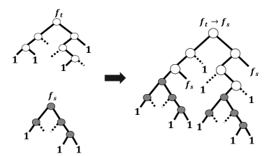
Lemma 7.
Given the encoding of from Lemma 6, we can polynomially reduce to some .
Proof. As mentioned earlier, is not necessarily an FBDD since it may contain various repeated variables within its diagram. We now show how each can be reduced to some .
We define each path as a concatenation of two subpaths , each corresponding the the relevant path in (or ) accordingly. Since each node corresponds to some input feature , we denote as a function that maps to its corresponding feature. We use the common conventions of , , and .
We now describe the following recursive algorithm for reducing to some .
-
1.
We traverse on all corresponding paths , starting from the root node and traversing downwards. The algorithm does not change as long as we are on the part of the traversion.
-
2.
Reaching a node , if for all it holds that , then we recursively continue traversing both left and right. Intuitively, this means that the feature corresponding to was not part of the decision path of .
-
3.
Otherwise, we reach some node such that there exists a in which . In this case, we delete from . We now need to connect the parent of with either the left or right child of within . Assume that for , or in other words leads to a right turn in the path . In this case, we connect the parent of with the right child of . If the opposite holds, i.e., leads to a left turn in the path , then we connect the parent of with the left child of .
Intuitively, when traversing over the second part of the path we can potentially come across two scenarios. In the first, we reach a feature within the path that did not participate in . In this case, we want to continue traversing both possible scenarios (leaving the corresponding feature in the tree). In the second case, we reach a feature that already participated in . In this scenario, we delete the corresponding node from and connect it in the same direction in which the corresponding feature is connected in .
Hence, at the end of this recursive process, we are left with an equivalent diagram where for each path , no two nodes exist, such that . Figure 4 depicts an illustration of this recursive process.
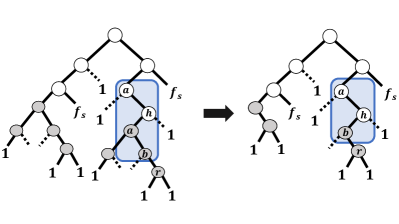
This concludes the proof that given two functions we can polynomially construct some , which is sufficient to show that is self-aligned.
Lemma 8.
The class is self-aligned.
Proof. We rely on Proposition 4 and show the corresponding encodings of and for (a sufficient condition for the self-alignment of the class). We start by showing how, given two functions over , we can polynomially construct a new function , such that . This will later imply the existence of the aforementioned logic relations. More formally:
Lemma 9.
Let , then can be constructed in polynomial time.
Proof. We assume that consists of hidden layers, while consists of hidden layers. We recall that our definition of an MLP is defined recursively, or in other words, is defined as:
| (25) |
and is defined as:
| (26) |
We now construct where . For fully formulating we need to formulate the associated weights and bias terms for each layer . Notice that is the input layer so no corresponding bias or weight is defined for them, and the dimensions of the input layers of both and are equal (for MLPs that receive inputs from the same domain).
Assuming that , we construct for all . In other words, is a concatenation of and . Notice that given that the dimensions of the hidden layers corresponding to are and the corresponding dimensions of the hidden layers corresponding to are , then the corresponding dimensions of the hidden layers of in this case are: .
Now, assuming that , without loss of generality, we can assume that . For any layer we construct in the same way, i.e., . For any we construct: . In other words, we concatenate the vector with a single bias term . In this particular case, the corresponding dimensions of are: .
Finally, we construct the weight vector . Again, for the case where , we construct it such that for any :
| (27) |
Assuming, without loss of generality, that , we construct it such that for any then is formalized as in Equation 27 and for any then:
| (28) |
Intuitively, the construction of the bias terms and the weight matrix layers captures a situation where we “stack” the hidden layers of and . This is a result of the concatenated bias vectors at each step, as well the fact that we zero out the effect of the weights corresponding to with those of , and vice versa.
Now, we describe the construction for the last layer of (recall that ). Since we focus on binary classification, the single activation function of the last layer can be considered, without loss of generality, as a step function. We also define the bias to be zero, i.e., . Now, we are left with defining the weight matrix of the last layer. Formally, we define , where each weight in is some strictly positive weight .
We now prove that the above encoding of satisfies that for any value :
Where (*) holds, since is directly connected to the outputs of both and (in which their step function was replaced by ReLU activations). This is the case both for when or, without loss of generality, when , replacing each corresponding weight in with a single neuron. Equivalence (**) holds directly from the definition of the step function (see Equation 12), while equivalence (***) holds from the fact that . Equivalence (****) follows from the fact that ReLU is a non-negative function.
We provide a visual illustration of this construction in Fig. 5. Note that the figure does not explicitly state the inner connections between and that are with zero weights.
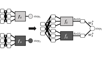
Now, based on Lemma 2, we know that MLPs are symmetrically constructible. In other words, given we can polynomially construct .
Since any logic gate can be encoded using the universal NOR gate, we can now polynomially construct both and . This can be done by recursively building the corresponding MLPs representing either the or constructions in a polynomial number of steps. Each one of these steps runs in polynomial time and outputs a new MLP of size at each step. Hence, we conclude that MLPs are self-aligned.
Next, we present the formalization of the Subset Sum problem, used for proving Proposition 4.
SSP (Subset Sum Problem): Input: set of positive integers, integer (such that ) and a (target) integer . Output: Yes, if there exists a subset of size such that , and No otherwise.
Proposition 4.
While the query MCR can be solved in polynomial time, the query MCR is NP-complete.
Proof. First, we briefly explain how it is possible to check whether a subset of features is contrastive for a Perceptron model, within the misaligned configuration, in polynomial time [12].
A Perceptron is defined by , where is the weight vector corresponding to the input x, and is the bias term. We can obtain the exact value of . Then, for the features in , it is possible to linearly find the assignments corresponding to the maximal and minimal values of . The maximal value is obtained by setting when and when . The minimal value is obtained respectively (setting when and when ). Now, we can calculate the entire range of possible values that can be obtained by setting the values of to x. If the minimal possible value is negative and the maximal possible value is positive then it means that is indeed contrastive, as there exists a subset of features that can alter the classification. If not, i.e., the entire range is either strictly positive or negative, this means that is not contrastive. More formally, is contrastive if and only if:
| (29) | |||
In other words, it holds that:
| (30) | |||
Membership. Given the aforementioned description regarding the polynomial validation of contrastive reasons for Perceptrons, membership in NP is straightforward, since one can guess a subset and validate whether it holds that , is contrastive with respect to , as well as the fact that . If these hold then we know that MCR.
Hardness. We reduce MCR from SSP (the Subset Sum problem), a classic NP-complete problem, previously formalized. Given some the reduction first checks the specific case where . In this scenario, we want to construct a “dummy” result. In other words, if , we can construct a “dummy” instance of . We define where and . We define such that and . In case that , we can simply construct a false encoding.
If this is not the case (meaning that ), the reduction constructs the two following Perceptrons and , where , , , and . The reduction constructs , and denotes a unit vector of size .
First, notice that there exists a contrastive reason of size for aligned by if and only if:
| (31) | |||
This means that there exists a subset of size such that:
| (32) | |||
We assume a valid encoding (since this can trivially be validated in polynomial time). The first “dummy” validation checks whether and . In such a case, it holds that . We also note that , which is of size (the entire input domain) is an aligned contrastive reason. This is due to the fact that and . Additionally, it holds that for any z it satisfies that . In other words:
| (33) | |||
Hence .
Thus, we can now assume that . Since all values in are negative, then it holds that for any subset of features :
| (34) |
It also clearly holds that for any :
| (35) |
Since we know that , and since these are negative integers, then there exists at least one integer in the complementary set , and hence it also holds that:
| (36) | |||
Regarding , since all of its values are positive, then it holds that:
| (37) |
Now, if , then there exists a subset of features of size such that . This indicates that:
| (38) | |||
as well as:
| (39) | |||
Regarding , it holds that:
| (40) | |||
and hence:
| (41) |
Given that , then there does not exist a subset of features of size such that . This is equivalent to saying that there does not exist a subset of features of size such that:
| (42) |
meaning that there does not exist a subset such that:
| (43) | |||
and hence: , concluding the reduction.
Theorem 5.
Assuming that , the class is not self-aligned.
Proof. Assume, by negation, that the model class is self-aligned. Hence, we deduce that given some we can polynomially construct a function such that if and only if . As we know from Proposition 4 that deciding is NP-hard and that is in PTIME, the following claim holds only if PTIME=NP. Hence, is not self-aligned.
Appendix E Framework Extenstions
Our framework can be extended in multiple axes. First, although we follow common conventions (e.g., [9, 12, 89, 15]) and focus on binary input and output domains to simplify our presentation, some of our findings are applicable to any discrete input or output domains. Additionally, rather than considering individual features, we can consider “high-level" features, e.g., by grouping multiple features together. This allows defining explanations, for example, in terms of super-pixels and also RGB images in various practical settings.
More broadly, the types of explanations analyzed in this work are explanations with formal and mathematical guarantees, commonly discussed within a sub-field of interest known as Formal XAI [68]. One benefit of explanations with formal guarantees is that, unlike heuristic-based explanations, they enable a more rigorous and mathematical analysis, allowing the study of computational complexity aspects of obtaining explanations [12, 13].
However, there exists a body of work in Formal XAI that focuses on the practical aspect of computing explanations with formal guarantees [25, 69, 13, 14, 47, 26, 27, 44, 51]. Initial efforts to compute such explanations were demonstrated on simple ML models, which allow tractable computations of explanations. These models include decision trees [53, 44], linear models [69], monotonic classifiers [70], and tree ensembles [50, 51, 11, 17]. More recently, various methods have been proposed to obtain explanations with formal guarantees for neural networks [61, 91, 14, 13, 42, 54]. This task is considered a computationally challenging one [12, 15]. However, the development of such methods is facilitated by the rapid advancement of neural network verification tools [57, 58, 90, 82, 65, 35, 98, 55, 60, 1, 22, 93, 94, 4], which are being developed more broadly to formally certify a diverse set of provable properties [23, 24, 66, 67, 78, 29, 18, 86, 30, 19, 2, 3, 5, 6, 71]. We believe that our work can serve as a step towards developing a more rigorous understanding of the potential capabilities and limitations of computing explanations with formal guarantees concerning a given distribution of interest.