Automated Techniques for Efficient Sampling of Piecewise-Deterministic Markov Processes

Abstract

Piecewise deterministic Markov processes (PDMPs) are a class of continuous-time Markov processes that were recently used to develop a new class of Markov chain Monte Carlo algorithms. However, the implementation of the processes is challenging due to the continuous-time aspect and the necessity of integrating the rate function. Recently, [11] proposed a new algorithm to automate the implementation of the Zig-Zag sampler. However, the efficiency of the algorithm highly depends on a hyperparameter ($t_{\textnormal{max}}$) that is fixed all along the run of the algorithm and needs preliminary runs to tune. In this work, we relax this assumption and propose a new variant of their algorithm that let this parameter change over time and automatically adapt to the target distribution. We also replace the Brent optimization algorithm by a grid-based method to compute the upper bound of the rate function. This method is more robust to the regularity of the function and gives a tighter upper bound while being quicker to compute. We also extend the algorithm to other PDMPs and provide a Python implementation of the algorithm based on JAX.

1 Introduction

Markov Chain Monte Carlo (MCMC) has been a cornerstone of simulation-based inference for the last 30 years. However, most of the methods are based on the Metropolis–Hastings algorithm, which create a reversible discrete-time Markov chains by adding a rejection step. This leads to a random walk behavior that can be inefficient in some settings. This analysis leads [16] to use a partial velocity refreshment for Hybrid Monte Carlo. At the end of the 1990s, some authors [14, 10] proposed new methods based on nonreversible Markov chains and showed that they could be more efficient than the reversible ones.

The idea of nonreversible Markov chains was further developed by physicists at the late 2000s and early 2010s, with different version of Event-Chain Monte Carlo [1, 20], first applied to the hard sphere model, or the work of [22].

Finally the idea of nonreversible Markov chains was developed by statisticians as an alternative to classical MCMC [15, 3, 17]. In the mid 2010s, a new family of MCMC algorithms was proposed, based on piecewise deterministic Markov processes (PDMPs) [12, 13]. [8] extended the Bouncy Particle Sampler which was originally proposed by [22]. The time discrete lifted Markov chain was extended to continuous time by [5] and then extended to multidimensional target by the Zig-Zag Sampler [4]. Both methods, Zig-Zag Sampler and Bouncy Particle Sampler, are time continuous and rejection-free. Then many other PDMP schemes were proposed, such as the Forward Event-Chain Monte Carlo [19], the Boomerang Sampler [7], the Coordinate Sampler [26] or the speedup Zig-Zag [25] among others.

The main drawback of PDMPs compared to time-discrete MCMC is the difficulty to sample them, due to the continuous-time aspect and the necessity to integrate the rate function. Several recent works have proposed methods to tackle this issue. For instance, [11, 23] propose new methods to construct upper bounds of the rate function to simulate the process, in a more automated way. This leads to an exact simulation of the process. Other lines of research are to approximate the process, for instance by discretizing it [2] or by using numerical solvers [21], while providing bounds on the error of the approximation.

The goal of this paper is to extend the automatic Zig-Zag algorithm from [11]. We propose a new method to tune automatically the hyperparameter $t_{\textnormal{max}}$ they use, and replace the computation of the maximum of the rate function by a grid-based method to obtain a piecewise constant upper bound. This method is more robust to the regularity of the function, which can be useful is the target distribution is not convex, while providing a tighter upper bound and a faster computation. We apply this new method to the Zig-Zag sampler but also other types of PDMPs. We provide a Python implementation of the algorithm based on JAX [9], making it easy to use and to extend to other PDMPs. It is available on GitHub at https://github.com/charlyandral/pdmp_jax on PyPI at https://pypi.org/project/pdmp-jax.

The outline of the paper is as follows. In Section 2, we present the general framework of PDMPs and some examples of PDMPs that will be used in the experiments. In Section 3, we present the automatic Zig-Zag sampler from [11] and analyze the role of the hyperparameter $t_{\textnormal{max}}$. In Section 4, we present our new method to adapt $t_{\textnormal{max}}$ and to compute the upper bound of the rate function, while providing a theoretical proof of the correctness of the method. In Section 5, we present the results of the experiments we conducted to compare the efficiency of the new method with the automatic Zig-Zag sampler.

2 Piecewise-deterministic Markov processes

2.1 Definition of a Piecewise-deterministic Markov processes

Let $\Pi$ be a probability measure on $\mathbb{R}^{d}$ that admits a density $\pi(x)$ with respect to the Lebesgue measure. We are interested in sampling from $\Pi$. Define $U(x)$ the potential of $\Pi$ defined such that $\pi(x)\propto\exp(-U(x))$. As for the Markov Chain Monte Carlo, the density needs only to be known up to a multiplicative constant, which means that the potential $U$ can be known up to an additive constant. This will not affect the process as the potential is only used through its gradient.

The space $\mathbb{R}^{d}$ for the location of the process is extended by adding a velocity component living in a velocity space $\mathcal{V}\subseteq\mathbb{R}^{d}$. This velocity space can be discrete (e.g. $\mathcal{V}=\{-1,1\}^{d}$) or continuous ($\mathcal{V}=\mathbb{R}^{d}$ or $\mathcal{V}=\mathbb{S}^{d-1})$.

The goal is to create a continuous-time process $Z_{t}=(X_{t},V_{t})$ on $\mathbb{R}^{d}\times\mathcal{V}$ that admits $\Pi$ as the first marginal of its invariant distribution $\rho(\mathrm{d}x\mathrm{d}v)$. More generally, a piecewise deterministic Markov process (PDMP) is a continuous-time Markov process defined by three elements:

1. A deterministic dynamics that follows the process between two events. This dynamics is defined by a differential equation $\partial_{t}Z_{t}=\Psi(Z_{t})$ for some function $\Psi$. To this ODE corresponds flow function $\phi_{t}(x,v)$ that gives the location of the process at time $t$ given its location and velocity at time 0. For instance, for the ZZS and the BPS, we have $\partial_{t}(X_{t},V_{t})=(V_{t},0)$ and thus $\phi_{t}(x,v)=(x+tv,v)$.

2. The rate of the events. The events are the jumps of the velocity of the process, while keeping the location constant. They correspond to the event of a time-inhomogeneous Poisson process with a rate function $\lambda(z)$. Using the flow function, we will write $\lambda(t;x,v)$ for $\lambda(\phi_{t}(x,v))$, or even $\lambda(t)$ if the starting point does not matter.

3. The transition kernel of the velocity. When an event occurs, the velocity jumps to a new value $v^{\prime}$ according to a transition kernel $Q(z,\mathrm{d}v^{\prime})$.

The extended generator of the process at $z=(x,v)$ is given by

$$\mathcal{L}f(z)=\nabla f(z)\cdot\Psi(z)+\lambda(z)\int_{\mathcal{V}}\left(f(x,v^{\prime})-f(x,v)\right)Q(z,\mathrm{d}v^{\prime})$$

Defining a PDMP is therefore equivalent to giving the triplet $(\phi_{t},\lambda,Q)$ (or $(\Psi,\lambda,Q)$).

2.2 Some examples of PDMPs

We quickly present some examples of PDMPs used for sampling that we will consider in the experiments, by giving the expression of $\lambda$, $\Psi$ and $Q$ for each of them.

2.2.1 The Zig-Zag sampler

We recall the expression of $\lambda$, $\Psi$ and $Q$ for the Zig-Zag sampler [4]. The velocity space is $\mathcal{V}=\{-1,1\}^{d}$, and its invariant measure is $\Pi\otimes\mathcal{U}(\mathcal{V})$. The deterministic dynamics is given by $\Psi(z)=(v,0)$ which corresponds to the flow function $\phi_{t}(x,v)=(x+tv,v)$. The rate function is given by

$$\lambda(x,v)=\sum_{i=1}^{d}(\nabla_{i}U(x)v_{i})_{+}=:\sum_{i=1}^{d}\lambda_{i}(x,v)$$

We denote $F_{m}(v)$ the velocity obtained by flipping the $m$-th component of $v$, e.g. For $v=(1,-1,1)$, $F_{2}(v)=(1,1,1)$. The transition kernel of the ZZS is given by

$$Q(x,v,\mathrm{d}v^{\prime})=\sum_{i=1}^{d}\frac{\lambda_{i}(x,v)}{\lambda(x,v)}\delta_{F_{i}(v)}(\mathrm{d}v^{\prime})$$

where $Q(x,v,\mathrm{d}v^{\prime})=\delta_{v}(\mathrm{d}v^{\prime})$ if $\lambda(x,v)=0$.

2.2.2 The Bouncy Particle sampler

For the Bouncy Particle Sampler [22, 8], the velocity space is $\mathcal{V}=\mathbb{R}^{d}$, and its invariant measure is $\Pi\otimes\mathcal{N}(0,I_{d})$. The deterministic dynamics is the same as for the ZZS, i.e. $\phi_{t}(x,v)=(x+tv,v)$. The rate function is given by:

$$\lambda(x,v)=\left\langle\nabla U(x),v\right\rangle_{+}+\underline{\lambda}$$

where $\underline{\lambda}$ is called the refreshment rate and is a constant that can be chosen to ensure the ergodicity of the process.

To define the transition kernel, we need to define the reflection operator. For $v\in\mathbb{R}^{d}$, the reflection operator $R_{v}$ is defined by $R_{v}(w)=w-2\frac{\left\langle w,v\right\rangle}{\left\langle v,v\right\rangle}v$ and corresponds to the reflection of $w$ with respect to the hyperplane orthogonal to $v$. The transition kernel of the BPS is given by

$$Q((x,v),\mathrm{d}v^{\prime})=\frac{\left\langle\nabla U(x),v\right\rangle_{+}}{\lambda(x,v)}\delta_{R_{\nabla U(x)}(v)}(\mathrm{d}v^{\prime})+\frac{\underline{\lambda}}{\lambda(x,v)}\mathcal{N}(\mathrm{d}v^{\prime};0,I_{d})$$

2.2.3 The Boomerang sampler

The Boomerang sampler [7] is a variation of the Bouncy Particle Sampler. The velocity space is $\mathcal{V}=\mathbb{R}^{d}$, and its invariant measure is $\Pi^{\prime}\otimes\mathcal{N}(0,I_{d})$, where $\Pi^{\prime}$ is the distribution with potential $U^{\prime}(x)=U(x)+\frac{1}{2}\left\langle x,x\right\rangle$. The deterministic dynamics is different from the BPS and is given by:

$$\phi_{t}(x,v)=(x\cos(t)+v\sin(t),-x\sin(t)+v\cos(t))$$

The rate function is the same as for the Bouncy Particle sampler : $\lambda(x,v)=\left\langle\nabla U(x),v\right\rangle_{+}+\underline{\lambda},$ for a refreshment rate $\underline{\lambda}$. The transition kernel is also the same as for the BPS.

2.2.4 Forward event-chain Monte Carlo

The forward event-chain (FEC) Monte Carlo [19] is a variation of the Bouncy Particle Sampler where the velocity jumps are not limited to bouncing. We will consider in the experiment the case where the velocity space is the sphere $\mathcal{V}=\mathbb{S}^{d-1}$ with the invariant distribution, such that the invariant measure of process is $\Pi\otimes\mathcal{U}(\mathcal{V})$. The dynamics is the same as for the BPS, i.e. $\phi_{t}(x,v)=(x+tv,v)$.

The rate function is given by $\lambda(x,v)=\left\langle\nabla U(x),v\right\rangle_{+}$ with no refreshment rate. The transition kernel is decomposed in two parts: one acts on the line directed by the gradient of the potential, and the other on its orthogonal. The article of [19] describe several possibilities for each part. For instance, one can choose to refresh to parallel component while slightly rotate the orthogonal part. This decomposition was also used in [24, 27].

2.3 Simulating PDMPs

As in most cases the integrator is defined in closed form, the main difficulty in simulating PDMPs is to simulate the time of the next event. For a process starting at $(x,v)$, the time of the next event is distributed as an exponential random variable with rate $\lambda(t;x,v)$. This can be simulated by drawing a random variable $u\sim\text{Exp}(1)$ and finding the time $\tau$ such that

$$\int_{0}^{\tau}\lambda(t;x,v)\mathrm{d}t=u.$$ (1)

In practice and in the general case, this integral cannot be computed analytically.

A way to circumvent this issue is to use the thinning algorithm. If we do not know how to integrate $\lambda$ but we know an upper bound $\Lambda$ such that $\lambda(t;x,v)\leq\Lambda(t)$ for all $t$ that we know how to integrate, the thinning algorithm gives us a way to simulate the time of the next event. We simulate the first event $\tau^{*}$ from a Poisson process with rate $\Lambda$. Then, we accept $\tau^{*}$ with probability $\lambda(\tau^{*})/\Lambda(\tau^{*})$. Otherwise, we simulate the next event from the Poisson process with rate $\Lambda$ and repeat the process.

Theorem 1.

[18] Let a Poisson point process with inhomogeneous rate $\Lambda(t)$ be such that $\lambda(t)\leq\Lambda(t)$ for all $t$. The thinning algorithm described above generates a Poisson point process with rate $\lambda(t)$.

3 The automatic Zig-Zag sampler from [11]

3.1 The algorithm

The main contribution of [11] is to automate the thinning algorithm by finding automatically the upper bound $\Lambda$ they choose to be constant $\Lambda\in\mathbb{R}$. As finding an upper bound for every $t$ is a difficult task, they propose to compute it only on an interval $[0,t_{\textnormal{max}}]$ and use it locally. This correspond to take for a process at position $(x,v)$ the upper bound

$$\Lambda=\max_{t\in[0,t_{\textnormal{max}}]}\lambda(t;x,v).$$

If the time of the next event computed using $\Lambda$ is larger than $t_{\textnormal{max}}$, the process move to $t_{\textnormal{max}}$ and the upper bound is recomputed. The hyperparameter $t_{\textnormal{max}}$ is fixed and needs to be tuned, and as they show in Figure 5 of their paper, its value has a great impact on the number of gradient evaluations and thus on the efficiency of the algorithm. The optimization on $t$ is done using Brent’s algorithm with a slight modification.

They make the assumption that the function is monotonic on the interval $[0,t_{\textnormal{max}}]$, which is a reasonable assumption for the rate function if you consider $t_{\textnormal{max}}$ small enough such that the process is only visiting one mode. Therefore they propose to check if the maximum is reached at $0$ or at $t_{\textnormal{max}}$ by doing only one iteration of the Brent’s algorithm. If it is the case they stop, otherwise they continue the optimization.

The full algorithm is presented in Algorithm 1 for the special case of Zig-Zag.

Input: Initial location $x_{0}$, initial velocity $v_{0}$, number of skeleton points $K$, rate functions $\lambda=\sum_{i=1}^{l}\lambda_{i}$,$t_{\textnormal{max}}$ the tuning parameter

Output: Time, location and velocity of the skeleton points

$t_{0}=0$, $k=1$

  # set starting time and skeleton count

$t=t_{0}$, $x=x_{0}$, $v=v_{0}$

  # set current state of the process

$\bar{\lambda}=\max_{t\in[0,t_{\textnormal{max}}]}{\lambda(t;x,v)}$

  # compute upper bound

$\tau^{*}\sim\text{Exp}(\bar{\lambda})$

  # propose switching time

$\tau^{opt}=\tau^{*}$

  # track time from last optimization

1 while $k\leq K$ do

       $u=0$

        # set acceptance to 0 until next proposal

2       while $\tau^{opt}\leq t_{\textnormal{max}}$ and $u=0$ do

             $\lambda(\tau^{opt})=\sum_{i=1}^{d}\lambda_{i}(\tau^{opt}:x,v)$

              # propose switching time

             $u\sim\text{Ber}(\lambda(\tau^{opt})/\bar{\lambda})$

              # accept or reject the proposal

3             if $u=1$ then

                   $m\sim\text{Multinom}\left(1:d,\left\{\frac{\lambda_{i}(\tau^{opt};x,v)}{\lambda(\tau^{*})}\right\}_{i=1}^{d}\right)$

                    # compute the global rate at $\tau^{opt}$

                   $t=t+\tau^{opt}$

                    # progress time

                   $x=x+\tau^{opt}v$

                    # progress location

                   $v=F_{m}(v)$

                    # flip the velocity of dimension $m$

                   $t_{k}=t$, $x_{k}=x$, $v_{k}=v$

                    # save skeleton point

                   $k=k+1$

                    # increment skeleton count

                   $\bar{\lambda}=\max_{t\in[t,t_{\textnormal{max}}]}{\lambda(t;x,v)}$

                    # compute new upper bound

                   $\tau^{*}\sim\text{Exp}(\bar{\lambda})$

                    # propose new switching time

                   $\tau^{opt}=\tau^{*}$

                    # reset time from last optimization

4                  

5            else

                   $\tau^{*}\sim\text{Exp}(\bar{\lambda})$

                    # propose new time increment

                   $\tau^{opt}=\tau^{opt}+\tau^{*}$

                    # compute new switching proposal

6                  

7            

8      if $\tau^{opt}>t_{\textnormal{max}}$ and $u=0$ then # if the horizon is reached with no flip

             $t=t+t_{\textnormal{max}}$

              # progress time to the horizon

             $x=x+t_{\textnormal{max}}v$

              # progress location until the horizon

             $v=v$

              # retain the velocity

             $\bar{\lambda}=\max_{t\in[0,t_{\textnormal{max}}]}{\lambda(t;x,v)}$

              # compute new upper bound

             $\tau^{*}\sim\text{Exp}(\bar{\lambda})$

              # propose new switching time

             $\tau^{opt}=\tau^{*}$

              # reset time from last optimization

9            

10      

return $\left\{t_{k},x_{k},v_{k}\right\}_{k=1}^{K}$

Algorithm 1 Automatic Zig-Zag sampler from [11]

3.2 Analysis of the role of the hyperparameter $t_{\textnormal{max}}$

The hyperparameter $t_{\textnormal{max}}$ is crucial for the efficiency of the algorithm, as seen before. In this section, we will interpret the influence of $t_{\textnormal{max}}$ in the two extreme cases where $t_{\textnormal{max}}$ is very small and very large.

3.2.1 Small $t_{\textnormal{max}}$ regime

When $t_{\textnormal{max}}$ is very small, the optimization when computing $\Lambda$ is done on a very small interval. Therefore, the function will not vary a lot and the upper bound by a constant will be rather sharp, which will lead to a good acceptance probability in the thinning algorithm. However, as the process is not allowed to move for a time longer than $t_{\textnormal{max}}$, the process will very often reach the horizon without flipping (the condition at line 1 of Algorithm 1 will be often true). The process will move in time by $t_{\textnormal{max}}$ and a new upper bound needs to be computed. This will lead to a lot of gradient evaluations in the optimization step while the process is barely moving.

3.2.2 Large $t_{\textnormal{max}}$ regime

When $t_{\textnormal{max}}$ is very large, the upper bound is computed over a large interval and gets very loose. This leads to a very low acceptance probability in the thinning algorithm. The process will often need to simulate a lot of events before accepting one. Each time, the computation of the rate for the accept/reject step (line 1 of the algorithm) requires gradient evaluations. As the upper bound is kept the same unless accepting or reaching the horizon, the loss of efficiency is in this case due to the low acceptance probability.

3.2.3 Counting the number of gradient evaluations

As detailed in the equation 12 of [11], the number of gradient evaluations can be decomposed in two parts. The first part is the number of gradient evaluations for the optimization of $\Lambda$, denoted $C^{\scriptscriptstyle\textnormal{opt}}$ and the second part is the number of gradient evaluations when computed the rate for the accept/reject step of the thinning algorithm, denoted $C^{\scriptscriptstyle\textnormal{tpp}}$.

The total number of gradient evaluations $C$ is given by

$$C^{\scriptscriptstyle\textnormal{top}}=C^{\scriptscriptstyle\textnormal{opt}}+C^{\scriptscriptstyle\textnormal{tpp}}.$$

The two regimes we have presented correspond to this trade-off. When $t_{\textnormal{max}}$ is small, $C^{\scriptscriptstyle\textnormal{opt}}$ is large and $C^{\scriptscriptstyle\textnormal{tpp}}$ is small, and when $t_{\textnormal{max}}$ is large, $C^{\scriptscriptstyle\textnormal{opt}}$ is small and $C^{\scriptscriptstyle\textnormal{tpp}}$ is large. Choosing the right value of $t_{\textnormal{max}}$ is therefore crucial to balance the two terms.

This is illustrated in Figure 1 where $C^{\scriptscriptstyle\textnormal{opt}}$ and $C^{\scriptscriptstyle\textnormal{tpp}}$ are plotted as a function of $t_{\textnormal{max}}$ for the Zig-Zag sampler, targeting a 30-dimensional standard Gaussian distribution.

Figure 1: Effect of $t_{\textnormal{max}}$ (in log-scale) on the number of gradient evaluations with the non-adaptive algorithm

3.3 The problem of optimization

The computation of the upper bound $\Lambda$ is done using Brent’s algorithm. However, in the cases where the target is multimodal, the resulting function $\lambda(t)$ may be non concave. In those cases the optimization part of the simulation may lead to a false upper bound. This results in a bias in the simulation of the events: as long as the upper bound $\Lambda$ is a true upper bound of $\lambda$, the procedure is correct. However, if $\Lambda$ is not an upper bound, the simulated process has not $\lambda$ as intensity. This issue was never addressed in the paper of [11], supposing that on a small scale (typically of length $t_{\textnormal{max}}$), the function is concave. However, one may be interested to simulate PDMPs on more general cases, where the function is not concave, for instance is the targets admits several modes close to each other. Replacing the Brent’s algorithm by another optimization algorithm, e.g. using the gradient of $\lambda$ may not solve the issue as the result may be stuck in a local maximum depending on the starting point.

3.4 Why $t_{\textnormal{max}}$ is constant ?

The hyperparameter $t_{\textnormal{max}}$, as it appears in the algorithm, is purely numerical. This was also noticed by [23]. It plays no role in the dynamics of the process, contrary to the standard deviation in a random walk Metropolis–Hastings algorithm for instance. It is only used to compute the upper bound $\Lambda$. Changing it each time the upper bound is recomputed will not change a thing, as soon as the optimization is successful.

Following this observation, we propose to let $t_{\textnormal{max}}$ change over the execution of the algorithm. To do so, we need to understand where the algorithm gets stuck in the two extreme cases we have presented.

First, if $t_{\textnormal{max}}$ is very small, the process will often reach the horizon without any event. This mean that the condition at line 1 of Algorithm 1 will be often true while never entering the inner while loop at line 1. In this case, we propose to increase $t_{\textnormal{max}}$ by multiplying it by a constant $\alpha>1$.

In the second case, $t_{\textnormal{max}}$ is very large, and all the budget is wasted in the thinning algorithm due to the low acceptance probability. The algorithm will rarely verify the condition of the if statement at line 1 and will mainly enter the else statement at line 1. Thus, in the else statement line 1, we propose to decrease $t_{\textnormal{max}}$ by dividing it by $\alpha$.

In both case, $t_{\textnormal{max}}$ is updated with a geometric rule. Therefore, even if the initial value of $t_{\textnormal{max}}$ is far from the optimal value, $t_{\textnormal{max}}$ will quickly adapt to the target distribution. One could use a different rule to update $t_{\textnormal{max}}$, for instance by making the adaptation decreasing over time. We found no need for this in our experiments. At some points, the two regimes will balance out and $t_{\textnormal{max}}$ will oscillate around the optimal value.

To illustrate the benefits of the adaptation, we redo the experiment of Figure 1 while letting $t_{\textnormal{max}}$ change over time, targeting again a 30-dimensional standard Gaussian distribution using a Zig-Zag sampler. We choose $\alpha=1.1$. The results are presented in Figure 2. We can see that the number of gradient evaluations is almost constant whatever the initial value of $t_{\textnormal{max}}$ is. Note that the range of $t_{\textnormal{max}}$ is also much larger than in the non-adaptive case.

Other possibilities to adapt $t_{\textnormal{max}}$ could be to use a quantile of the time between events, as proposed by [23]. We will not investigate this possibility here.

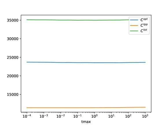
Figure 2: Effect of $t_{\textnormal{max}}$ (in log-scale) on the number of gradient evaluations with the adaptive algorithm

4 New general method: using a grid

4.1 New computation of the upper bound

The thinning theorem is valid for a constant upper bound, which makes the computation of the Poisson point process very easy, but it is not necessary. The method we propose in this paper is to replace a constant upper bound by a piecewise constant one. Having a piecewise constant function makes the equation (1) still very easy to solve. Typically, the function will be constant over a grid. This methods presents two main advantages.

First, this method outputs a tighter upper bound that using a constant. Thus, using it in the thinning algorithm will lead to a much higher acceptance probability.

Second, this computation is much robust to the regularity of the function. If the grid is fine enough (compared to the regularity of the function), the upper bound will be correct, even if the function is not concave, resolving an issue of the original algorithm.

Leveraging the possibilities offered by the python library JAX [9], and in particular the vectorization, we can evaluate the rate function $\lambda$ on a grid very effectively, compared to an optimization algorithm where the function is evaluated one at a time. Therefore, even if the total number of evaluations may be larger that doing a classic optimization step, the computation time may be shorter due to the vectorization. Also, compared to a classic optimization algorithm, where only the last evaluation is used, we use all the evaluations of the rate function to construct the bound. We also leverage the automatic differentiation in JAX, not only to compute the gradient of the potential, but also to compute the derivative of the rate function.

4.2 Construction of the upper bound

We now present the construction of the piecewise constant upper bound for a given function $\lambda$ that is suppose to be differentiable. As for the automatic Zig-Zag algorithm, we compute an upper bound on an interval $[0,t_{\textnormal{max}}]$, for a given point $(x,v)$. We introduce a new hyperparameter $N$ that is the number of segments in the grid. By default, we divide the interval $[0,t_{\textnormal{max}}]$ in $N$ equal segments $[t_{i},t_{i+1}]:=[\frac{i}{N}t_{\textnormal{max}},\frac{i+1}{N}t_{\textnormal{max}}]$ for $i=0,\dots,N-1$. Then, we construct an upper bound of $\lambda$ on each segment, as follows.

On a given segment $[t_{i},t_{i+1}]$ we have at our disposal four pieces of information: $\lambda(t_{i};x,v)$, $\lambda(t_{i+1};x,v)$ and their time derivatives $\lambda^{\prime}(t_{i};x,v)$ and $\lambda^{\prime}(t_{i+1};x,v)$, that we will denote respectively $y_{i}$, $y_{i+1}$, $d_{i}$ and $d_{i+1}$ for simplicity. The upper bound on the segment, denoted $\Lambda_{i}$ is taken to be the maximum of the three values : $y_{i}$, $y_{i+1}$, and the y-axis of the intersection of the two tangents at $t_{i}$ and $t_{i+1}$, called $m_{i}$. The first two values are most relevant where the function is monotonic and the last one $m_{i}$, depending on the derivatives, is used to capture the case where the function reaches a local maximum on the segment. This is illustrated in Figure 3 where the function is the sine function, neither concave nor convex.

More precisely, the intersection point $(x_{i},m_{i})$ is solution to the system of equations :

$$\begin{cases}m_{i}=d_{i}x_{i}+y_{i}-d_{i}t_{i}\\ m_{i}=d_{i+1}x_{i}+y_{i+1}-d_{i+1}t_{i+1}\end{cases}$$ (2)

This gives $x_{i}=\frac{y_{i+1}-y_{i}+d_{i}t_{i}-d_{i+1}t_{i+1}}{d_{i}-d_{i+1}}$ and $m_{i}=d_{i}x_{i}+y_{i}-d_{i}t_{i}$. A simplification is made: if $d_{i}=d_{i+1}$, $x_{i}=t_{i}$ and $m_{i}=y_{i}$. If $x_{i}$ does not lie in the interval, we clip it to the bounds. The upper bound on the segment is then $\Lambda_{i}=\max(y_{i},y_{i+1},m_{i})$.

Finally, on the whole interval $[0,t_{\textnormal{max}}]$, the upper bound $\Lambda$ can be expressed as $\Lambda(t)=\sum_{i=0}^{N-1}\Lambda_{i}\mathbbm{1}_{[t_{i},t_{i+1})}(t)$. This procedure is summarized in Algorithm 2. Given a function $\lambda$, an horizon $t_{\textnormal{max}}$ and a number of segments $N$, we denote $\textsf{UpperBound}(\lambda,t_{\textnormal{max}},N)$ the function that returns the upper bound $\Lambda$ using Algorithm 2 and the grid $(t_{i})_{i=0}^{N}=(\frac{it_{\textnormal{max}}}{N})_{i=0}^{N}$.

Input: the function $\lambda:\mathbb{R}\to\mathbb{R}$ to upper bound, an horizon $t_{\textnormal{max}}$, a number of segments $N$

Output: the upper bound $\Lambda$ of $\lambda$

1

2for $i=0$ to $N-1$  do

3       $t_{i}=\frac{i}{N}t_{\textnormal{max}}$

       $y_{i}=\lambda(t_{i})$

        # evaluate the function and its derivative on the grid

4       $d_{i}=\lambda^{\prime}(t_{i})$

5      

6for $i=0$ to $N-1$ do

7      

8      if $d_{i}=d_{i+1}$ then

9             $x_{i}=t_{i}$

10             $m_{i}=y_{i}$

11            

12      else

             $x_{i}=\frac{y_{i+1}-y_{i}+d_{i}t_{i}-d_{i+1}t_{i+1}}{d_{i}-d_{i+1}}$

              # abscissa of the intersection of the two tangents

             $x_{i}=\min(t_{i+1},\max(t_{i},x_{i}))$

              # clip $x_{i}$ to the bounds

13             $m_{i}=d_{i}x_{i}+y_{i}-d_{i}t_{i}$

14      $\Lambda_{i}=\max(y_{i},y_{i+1},m_{i})$

15      

16$\Lambda(t)=\sum_{i=0}^{N-1}\Lambda_{i}\mathbbm{1}_{[t_{i},t_{i+1})}(t)$

17 return $\textsf{UpperBound}(\lambda,t_{\textnormal{max}},N):=\Lambda$

Algorithm 2 UpperBound: construction of the upper bound

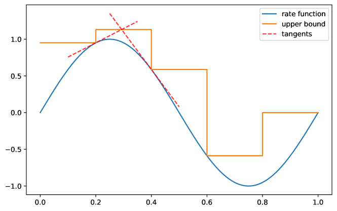
Figure 3: Construction of the upper bound for the sine function

4.3 Correctness of the upper bound

We will now show under which conditions the upper bound $\Lambda$ constructed in Algorithm 2 is indeed an upper bound of $\lambda$. Define

$$Z=\{t\in(0,t_{\textnormal{max}}):(\lambda^{\prime}(t)=0\text{ and }\lambda^{\prime\prime}(t)<0)\text{ or }\lambda^{\prime\prime}(t)=0\},$$

the set containing the critical points of $\lambda$ that are (local) maxima, henceforth referred to as maximum critical points (they may also be a zero of the second derivative), and the zeros of its second derivative that are not maximum critical points. We also define the minimum distance between two points of $Z$ as

$$\delta=\min_{t,t^{\prime}\in Z,t\neq t^{\prime}}|t-t^{\prime}|.$$

Remark 1.

If the set $Z$ is infinite, typically if the first or second derivative cancel out on an interval, we can replace the set $Z$ by its quotient by the equivalence relation $t\sim t^{\prime}$ if $t$ and $t^{\prime}$ are in the same connected component of $Z$. The condition $t\neq t^{\prime}$ in the definition of $\delta$ now means that $t$ and $t^{\prime}$ are not connected.

Remark 2.

The intuition behind the definition of $Z$ is that, in order to have an upper bound, a local maximum and a change of concavity cannot happen on the same subinterval. This ensures that around a local maximum the function is concave and thus under its tangents. If it not the case, one can easily construct a smooth function for which the function constructed in Algorithm 2 is not an upper bound due to the inflection point.

Now that the set $Z$ as well as the minimum distance between its points $\delta$ are defined, we can state the main theorem for the correctness of the upper bound.

Theorem 2.

Let $\lambda:[0,t_{\textnormal{max}}]\to\mathbb{R}$ be a twice continuously differentiable function such that $\delta>0$. Suppose that $\max_{i=0,\dots,N-1}|t_{i+1}-t_{i}|<\delta$.

Then, the function $\Lambda$ constructed in Algorithm 2 is an upper bound of $\lambda$, i.e. for all $t\in[0,t_{\textnormal{max}}]$, $\Lambda(t)\geq\lambda(t)$.

Proof.

Let $t\in[0,t_{\textnormal{max}}]$. We will show that $\Lambda(t)\geq\lambda(t)$. Let $i$ be such that $t\in[t_{i},t_{i+1})$. By construction of $Z$ and the grid, we have that $(t_{i},t_{i+1})$ contains at most one point of $Z$. Thus we have two cases to consider: the interval $(t_{i},t_{i+1})$ contains no maximum critical point of $\lambda$, or it contains one.

If $(t_{i},t_{i+1})$ contains no maximum critical point of $\lambda$, then, because $\lambda$ is differentiable on $(t_{i},t_{i+1}]$, it reaches its maximum at the bounds of the interval. Therefore, $\lambda(t)\leq\max(y_{i},y_{i+1})\leq\Lambda(t)$.

Second case, $(t_{i},t_{i+1})$ contains a unique maximum critical point $s$ of $\lambda$. By definition of $Z$, $\lambda^{\prime\prime}\neq 0$ on $(t_{i},t_{i+1})\backslash\{s\}$ and as $\lambda^{\prime\prime}$ is continuous, this implies that $\lambda^{\prime\prime}$ does not change sign on $(t_{i},t_{i+1})$ and thus that $\lambda^{\prime}$ is monotonic on $(t_{i},s]$ and $[s,t_{i+1})$. As $s$ is a local maximum, $\lambda^{\prime}$ is decreasing on a neighborhood of $s$. Combining this with the previous argument, we have that $\lambda^{\prime}$ is decreasing on $(t_{i},t_{i+1})$ and thus $\lambda$ is concave on $(t_{i},t_{i+1})$. The graph of $\lambda$ is then under its tangents. As the two tangents at $t_{i}$ and $t_{i+1}$ respectively have slopes of different signs, the ordinate of the intersection of the two tangents is larger than $\lambda(s)$ the local maximum. Thus, $\Lambda(t)\geq\lambda(t)$.

∎

Remark 3.

In the specific case of PDMPs where the potential is convex and twice differentiable, the rate function is non decreasing and algorithm 2 will therefore always output a correct upper bound, even for $N=2$. Indeed , if the rate function is like $\lambda(t)=\left\langle\nabla U(x+tv),v\right\rangle_{+}+\underline{\lambda}$ (for the Bouncy Particle or the Forward Event Chain), then the derivative of $\left\langle\nabla U(x+tv),v\right\rangle$ is $\left\langle\nabla^{2}U(x+tv)v,v\right\rangle$, which is positive as the Hessian is positive semi-definite.

If the rate function is like $\lambda(t)=\sum_{i=1}^{d}(\nabla_{i}U(x+tv)v_{i})_{+}$ (for the Zig-Zag sampler), then the derivative of $\nabla_{i}U(x+tv)v_{i}$ is $\left\langle\nabla^{2}U(x+tv)v,e_{i}\right\rangle v_{i}=\sum_{j}\frac{\partial^{2}U}{\partial x_{i}x_{j}}(x+tv)v_{j}v_{i}$. Thus, for a Zig-Zag velocity and if the Hessian is diagonally dominant, $\sum_{j}\frac{\partial^{2}U}{\partial x_{i}x_{j}}(x+tv)v_{j}v_{i}>0$ and the rate function is increasing. This condition on the Hessian is not just a technical condition, and it was discussed in the Gaussian case in [6].

4.4 Use of the upper bound in the case of PDMPs sampling

In the case of PDMP sampling, the rate function of the vast majority of processes is either the rate of the Zig-Zag Sampler $\lambda_{\text{ZZ}}(x,v)=\sum_{i=1}^{d}(\nabla_{i}U(x)v_{i})_{+}$ or the rate of the Bouncy Particle Sampler $\lambda_{\text{BPS}}(x,v)=\left\langle\nabla U(x),v\right\rangle_{+}+\underline{\lambda}$. The easy solution would be to use the algorithm 2 directly on $\lambda_{\text{ZZ}}$ or $\lambda_{\text{BPS}}$. However, the positive part in the rate function makes the function non differentiable even if the potential $U$ is smooth, leading to errors in the bound. We thus propose two solutions to overcome this issue depending on the rate function.

4.4.1 Case of a Bouncy Particle-like rate

If the process has a rate function of the form $\lambda_{\text{BPS}}(t)=\left\langle\nabla U(x_{t}),v_{t}\right\rangle_{+}+\underline{\lambda}$, we can use the algorithm 2 directly on $\left\langle\nabla U(x_{t}),v_{t}\right\rangle$ instead of $\lambda_{\text{BPS}}$. The function $t\mapsto\left\langle\nabla U(x_{t}),v_{t}\right\rangle$ is smooth and thus the bound has more chances to be correct. If $\tilde{\Lambda}$ is an upper bound for $\left\langle\nabla U(x_{t}),v_{t}\right\rangle$ on $[0,t_{\textnormal{max}}]$, then $(\tilde{\Lambda})_{+}(t)+\underline{\lambda}$ is an upper bound for $\lambda_{\text{BPS}}(t)$ on $[0,t_{\textnormal{max}}]$. We call this method the signed strategy.

The main benefit of this approach is its ability to retain the gradient information even when $\lambda_{\text{BPS}}$ is negative, rather than having a zero gradient due to the positive part. For instance, if the true rate function is concave and positive on a interval smaller than the grid, computing the upper bound of $\lambda_{\text{BPS}}$ will fail, while computing the upper bound of $\left\langle\nabla U(x_{t}),v_{t}\right\rangle$ will be correct.

4.4.2 Case of a Zig-Zag-like rate

If the function has a rate function of the form $\lambda_{\text{ZZ}}(t)=\sum_{j=1}^{d}(\nabla_{j}U(x_{t})v_{t,j})_{+}$, the problem is more complex. While in the previous case, the rate had only one point of non differentiability, always where the rate function equals to zero, the rate function of the Zig-Zag sampler has non differentiability points that can be at any positive value. Computing the upper bound of $\left\langle\nabla U(x_{t}),v_{t}\right\rangle$ will not work in this case because some terms of $\sum_{j=1}^{n}\nabla_{j}U(x_{t})v_{t,j}$ may be negative and thus cancel each other.

However, we can leverage the vectorized form of the rate function to compute the upper bound of each term separately. This defines the vectorized strategy, which again we can subdivide in two cases : signed and not signed.

In the vectorized and not signed strategy, we compute the upper bound of each term of $\lambda_{\text{ZZ}}$ separately, i.e. we compute an upper bound for $t\mapsto(\nabla_{j}U(x_{t})v_{t,j})_{+}$, for $j=1,\dots,d$. Then we take the sum of those upper bounds as the upper bound of $\lambda_{\text{ZZ}}$.

In the vectorized signed strategy, we compute the upper bound of each term separately and without taking their positive parts, i.e. we compute an upper bound $\Lambda_{j}$ for $t\mapsto\nabla_{j}U(x_{t})v_{t,j}$, for $j=1,\dots,d$. Then, we take the sum of the positive parts of the upper bounds: $\sum(\Lambda_{j})_{+}\geq\lambda$ This method is the most robust to the non differentiability of the rate function, but may lead to a slightly looser upper bound.

4.4.3 Computing the next event

Once the upper bound $\Lambda$ is computed, the time of the next event can be simulated by integrating $\Lambda$. Given $e\sim\text{Exp}(1)$, because the upper bound is piecewise constant, finding $\tau$ such that $\int_{0}^{\tau}\Lambda(t)\mathrm{d}t=e$ can be solved easily. We denote $i$ the index such that $\int_{0}^{t_{i}}\Lambda(t)\mathrm{d}t\leq u<\int_{0}^{t_{i+1}}\Lambda(t)\mathrm{d}t$. Then, $\tau=t_{i}+\frac{e-\int_{0}^{t_{i}}\Lambda(t)\mathrm{d}t}{\Lambda(t_{i})}$. The algorithm is presented in Algorithm 3.

Input: Upper bound $\Lambda$, number of segments $N$, horizon $t_{\textnormal{max}}$, a time $e$

Output: Time of the next event $\tau$

1 $i=0$

2 while $\int_{0}^{t_{i}}\Lambda(t)\mathrm{d}t\leq e$ and $i<N$ do

3       $i=i+1$

4      

5if $i=N$ then

       $\tau=t_{\textnormal{max}}+1$

        # the horizon is reached

6      

7else

8       $\tau=t_{i}+\frac{u-\int_{0}^{t_{i}}\Lambda(t)\mathrm{d}t}{\Lambda(t_{i})}$

9      

return $\textsf{NextEvent}(\Lambda,t_{\textnormal{max}},N,e):=\tau$

Algorithm 3 NextEvent : computation of the time of the next event

4.5 Adaptation of tmax in this case

The adaptation strategy of $t_{\textnormal{max}}$ presented in Section 3.4 can be used in this case. It is slightly modified to restrain the value of $t_{\textnormal{max}}$, as having a too large value of $t_{\textnormal{max}}$ may lead to errors in the upper bound. Instead of multiplying and dividing $t_{\textnormal{max}}$ by the same constant $\alpha$, we propose to multiply $t_{\textnormal{max}}$ by $\alpha_{+}$ if the horizon is reached without any event and to divide by $\alpha_{-}$ if an event is rejected.

With this strategy, we noticed in the experiments that the ratio $\frac{\alpha_{+}-1}{\alpha_{-}-1}$ is connected to the ratio between the number of time the horizon is reached and the number of events that are rejected. If $\alpha_{+}=\alpha_{-}$, the horizon is reached approximately as often as the events are rejected. If the ratio is $1/4$ (for instance we decrease $t_{\textnormal{max}}$ by $4\%$ and increase it by $1\%$), the horizon is reached approximately four times more often than the events are rejected.

4.6 Algorithm for the PDMP

The algorithm 1 adapted to use the upper bound $\Lambda$ constructed in Algorithm 2 is presented in Algorithm 4. It is extended to the general case of PDMPs, defined by the triplet integrator, intensity rate, jump kernel $(\phi_{t},\lambda,Q)$. It includes the adaptation of $t_{\textnormal{max}}$ as presented in the previous section, and parametrized by $\alpha_{+}$ and $\alpha_{-}$.

Input: Initial location $x_{0}$, initial velocity $v_{0}$, number of skeleton points $K$, rate functions $\lambda$,initial horizon $t_{\textnormal{max}}$, number of segments for the grid $N$, integrator $\phi_{t}$, velocity jump kernel $Q$, adaptation parameters $\alpha_{+}$ and $\alpha_{-}$

Output: Time, location and velocity of the skeleton points

$t_{0}=0$, $k=1$

  # set starting time and skeleton count

$t=t_{0}$, $x=x_{0}$, $v=v_{0}$

  # set current state of the process

$\Lambda=\textsf{UpperBound}(\lambda(\,\cdot\,;x,v),t_{\textnormal{max}},N)$

  # compute upper bound using Algorithm 2

1 $e\sim\text{Exp}(1)$

$\tau^{*}=\textsf{NextEvent}(\Lambda,t_{\textnormal{max}},N,e)$

  # propose switching time using Algorithm 3

$\tau^{opt}=\tau^{*}$

  # track time from last optimization

2 while $k\leq K$ do

       $u=0$

        # set acceptance to 0 until next proposal

3       while $\tau^{opt}\leq t_{\textnormal{max}}$ and $u=0$ do

             $u\sim\text{Ber}(\lambda(\tau^{opt})/\Lambda(\tau^{opt}))$

              # accept or reject the proposal

4             if $u=1$ then

                   $t=t+\tau^{opt}$

                    # progress time

                   $x,v=\phi_{\tau^{opt}}(x,v)$

                    # progress location and velocity

                   $v\sim Q(x,v,\,\cdot\,)$

                    # velocity jump

                   $t_{k}=t$, $x_{k}=x$, $v_{k}=v$

                    # save skeleton point

                   $k=k+1$

                    # increment skeleton count

                   $\Lambda=\textsf{UpperBound}(\lambda(\,\cdot\,;x,v),t_{\textnormal{max}},N)$

                    # compute new upper bound

5                   $e\sim\text{Exp}(1)$

                   $\tau^{*}=\textsf{NextEvent}(\Lambda,t_{\textnormal{max}},N,e)$

                    # propose new switching time

                   $\tau^{opt}=\tau^{*}$

                    # reset time from last optimization

6                  

7            else

8                   $e^{\prime}\sim\text{Exp}(1)$

9                   $e=e+e^{\prime}$

                   $t_{\textnormal{max}}=\alpha_{-}\cdot t_{\textnormal{max}}$

                    # decrease horizon

                   $\tau^{opt}=\textsf{NextEvent}(\Lambda,t_{\textnormal{max}},N,e)$

                    # compute new switching proposal

10                  

11            

12      if $\tau^{opt}>t_{\textnormal{max}}$ and $u=0$ then # if the horizon is reached with no flip

             $t=t+t_{\textnormal{max}}$

              # progress time to the horizon

             $x,v=\phi_{t_{\textnormal{max}}}(x,v)$

              # progress location until the horizon

             $t_{\textnormal{max}}=\alpha_{+}\cdot t_{\textnormal{max}}$

              # increase horizon

             $\Lambda=\textsf{UpperBound}(\lambda(\,\cdot\,;x,v),t_{\textnormal{max}},N)$

              # compute new upper bound

13             $e\sim\text{Exp}(1)$

             $\tau^{*}=\textsf{NextEvent}(\Lambda,t_{\textnormal{max}},N,e)$

              # propose new switching time

             $\tau^{opt}=\tau^{*}$

              # reset time from last optimization

14            

15      

return $\left\{t_{k},x_{k},v_{k}\right\}_{k=1}^{K}$

Algorithm 4 PDMP sampler with automatic tuning of $t_{\textnormal{max}}$ and piecewise constant upper bound

4.7 Dealing with errors in the upper bound

The upper bound constructed in Algorithm 2 is not always an upper bound of the rate function. This can occurs when the function is not differentiable, or when the grid is not fine enough. In this case, the algorithm will not be exact. The only way to spot this issue is the algorithm is to check if the acceptance rate for the thinning algorithm is larger than $1$. This is a sign that the upper bound is wrong However, having no event is not a sign that the upper bound is correct, even if it provides a feedback on the quality of the bound.

In practice, we deal with the issue the same way as in the implementation of the automatic Zig-Zag [11]. When computing the ratio $\lambda(\tau^{opt})/\Lambda(\tau^{opt})$ in the algorithm, if it is larger than $1$, we redo the computation of the upper bound with an horizon $t_{\textnormal{max}}$ divided by two.

5 Numerical experiments

To illustrate the benefits of this new methods, we will compare it to the automatic Zig-Zag algorithms on two examples. The implementation of the algorithms is done in Python using the JAX library [9]. It is available on GitHub at https://github.com/charlyandral/pdmp_jax on PyPI at https://pypi.org/project/pdmp-jax. All the experiments were done on CPU with a Apple M1 chip.

5.1 Mixture of two Gaussian distributions with different scales

For the first example, we consider a mixture of two Gaussian distributions in dimension 2. The target distribution is $\Pi=\frac{1}{2}\mathcal{N}((0,0),I_{2})+\frac{1}{2}\mathcal{N}((1,1),\sigma^{2}I_{2})$, with $\sigma=0.03$. While the two modes are close to each other, this target can be complicated to sample from because of the second mode that is peaked. The different of scale in the two modes makes difficult to find a good horizon $t_{\textnormal{max}}$ for the entire space. If the horizon $t_{\textnormal{max}}$ is too large, the peaked mode can easily be missed, while if it is at the scale of $\sigma$, the process will be slow to move in the first mode. An easy way to diagnose this issue is to look at the mean of the sample obtained. If the second mode is not visited, the means (of each component) will be smaller that the true mean $(0.5,0.5)$.

For this example, we will use the Bouncy Particle Sampler with a refresh rate of $0.1$. We first compare the effect of the horizon $t_{\textnormal{max}}$ and of the number of grid points on the mean of the sample. The two adaptation parameters are set to $\alpha_{+}=1.01$ and $\alpha_{-}=1.04$. We used the signed strategy from section 4.4.1 to compute the upper bound.

We compare four values of $t_{\textnormal{max}}$ : $0$, $0.01$, $0.1$ and $1$, where $0$ means that the horizon is adapted and for the three other values, the horizon is fixed with no adaptation. We also consider six values of the number of grid points $N$ : $0$, $5$, $10$, $20$, $50$ and $100$. Here, $0$ means that the upper bound is computed using the Brent algorithm as for the automatic Zig-Zag algorithm. In this specific case, only the default strategy is used (not vectorized not signed). We run $10$ different processes of $1$M skeleton points for each combination of $t_{\textnormal{max}}$ and $N$. The mean of the process is computed analytically from the skeleton points. The results are presented in Figure 4.

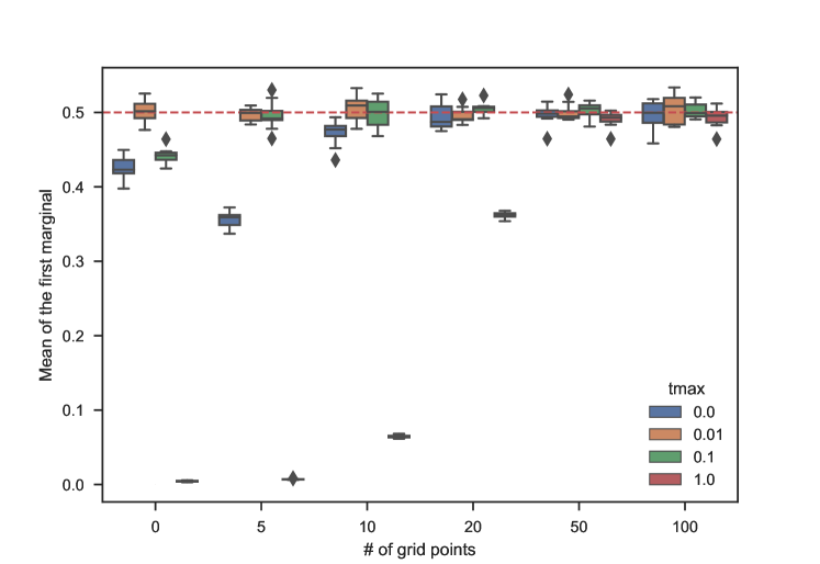
Figure 4: Mean of the sample for the mixture of Gaussian distributions as a function of $t_{\textnormal{max}}$ and $N$

We see that for a small grid, or for an optimization-based bound, the mean of the process is far from the true mean if the horizon is not very small. For instance, using the Brent algorithm and $t_{\textnormal{max}}=1.$ give a mean of almost zeros on the 10 runs, meaning that the narrow mode is missed each time. The adaptation of the horizon fails in the case the produce an unbiased result. However, using a grid with a sufficient number of points (here $>20$), the mean of the samples is around its true value.

Finally, we look at the computation time of the algorithm for the different values of $t_{\textnormal{max}}$ and $N$. The results are presented in Figure 5. One first observation is that the choice of $t_{\textnormal{max}}=0.01$ regardless of the number of grid points, is much slower than the other choices. This balances the fact that looking only at Figure 4, $t_{\textnormal{max}}=0.01$ was a good choice. This can be easily explained in this case by the fact that when using a small $N$, $t_{\textnormal{max}}$ must be small to capture the narrow mode. However, this makes the algorithm not efficient while moving in the broad mode.

The figure also shows that computing the bound using the Brent’s algorithm is much slower than using a grid, even for $100$ points. This relates to the fact that evaluating the rate function on a grid is much faster than using an optimization algorithm where the evaluations are done one at a time. Finally, the adaptation of $t_{\textnormal{max}}$ is very efficient in this case for a grid as it is one of the fastest method compared to the other choices of $t_{\textnormal{max}}$. It is worth noting that this is not the case for the Brent’s algorithm, where the adaptation is slower than using a fixed $t_{\textnormal{max}}$. We have not investigated the reason for this behavior.

Overall, choosing $N=50$ (or even $N=20$) and adapting $t_{\textnormal{max}}$ gives the best results in terms of computation time and accuracy of the sample : it produces an correct sample for a fraction (around $10\%$) of the time used by the automatic Zig-Zag algorithm with $t_{\textnormal{max}}=0.01$.

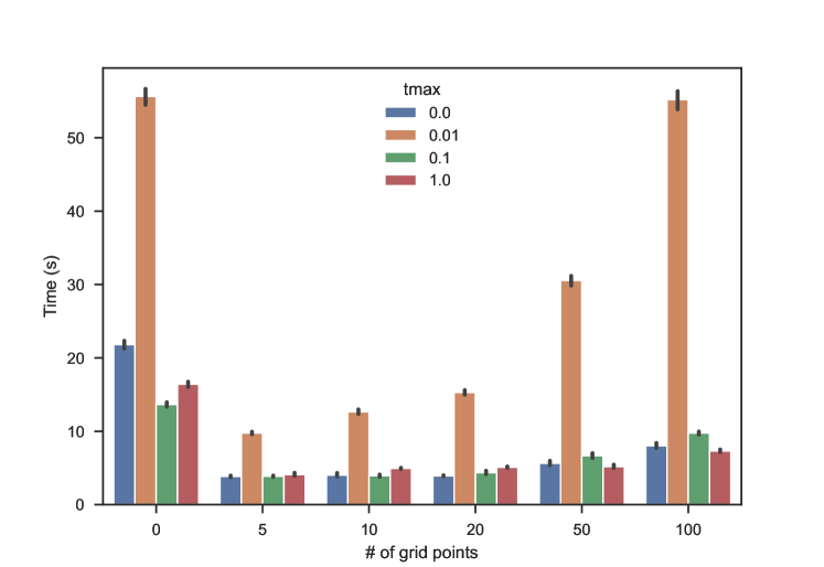
Figure 5: Mean computation time of the skeleton for the mixture of two Gaussian distributions with different scales as a function of $t_{\textnormal{max}}$ and $N$

5.2 Local mixture of 20 Gaussian distributions

For this second example, we consider a mixture of $20$ Gaussian distributions in dimension $2$. It is constructed as follows: for each $i=1,\dots,20$, we sample a mean $\mu_{i}$ from a Gaussian in $\mathbb{R}^{2}$ with variance $3^{2}$. The target distribution is then $\Pi=\frac{1}{K}\sum_{i=1}^{K}\mathcal{N}(\mu_{i},I_{d})$. This constructs a non-convex potential that can be difficult to bound. The sampling of the means is done once at the beginning of the experiment and is kept fixed across the different runs.

We use this target to evaluate the errors in the upper bound, and to illustrate the effect of the computations tricks described in sections 4.4.1 and 4.4.2

5.2.1 Results for the Zig-Zag sampler

We first consider the Zig-Zag sampler. The horizon $t_{\textnormal{max}}$ is set to be adaptive with $\alpha_{+}=1.01$ and $\alpha_{-}=1.04$. We compare the results using different grid sizes $N$ ($5,10,20,50$) and the Brent’s algorithm ($N=0$ in the figures by convention). We also compare the strategies of section 4.4.2. There are three strategies:

• Computing the upper bound of $\lambda_{\text{ZZ}}$ directly. We refer to this strategy as no vectorized and no signed.

• Computing the upper bound on each term of the rate $(\nabla_{i}U(x_{t})v_{t,i})_{+}$ separately. We called this strategy vectorized but not signed.

• Computing the upper bound of $\nabla_{i}U(x_{t})v_{t,i}$ separately, and taking the positive part on the bound. We refer to this strategy as vectorized and signed.

To measure the errors, we look at two quantities: the number of times that the acceptance rate of the thinning algorithm is larger than $1$, and its mean value in this case, to which we subtract $1$ to get a value close to $0$. We run $20$ different processes for each combination of $N$ and the strategy, again with $1$M skeleton points each, except for $N=0$ where only the no vectorized and no signed strategy is used. The results are presented in Figure 6.

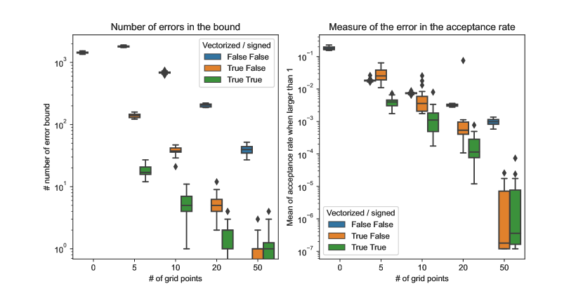
Figure 6: Measure of the errors in the Zig-Zag sampler for the mixture of 20 Gaussian distributions depending on the grid size and the bounding strategy. The left plot shows the number of times the acceptance rate is larger than $1$, in log scale. The right plot shows the mean value of the acceptance rate when it is larger than $1$, minus $1$, in log scale.

The results shows again that using the Brent’s algorithm is not efficient in terms of errors. The more grid points, the less errors in the upper bound. The different strategies also have an impact on the errors, as we may expect. Taking the more advanced strategy (vectorized and signed) gives the best results in terms of errors. It is followed by the vectorized but not signed strategy, and finally the no vectorized and no signed strategy. Also, we see that the distance of the error to $1$ (right plot) is also greatly reduced when using the vectorized and signed strategy.Therefore, in addition to having less errors, the errors are also smaller, allowing us to think that the upper bound is more more accurate when it is off, which should lead to a less biased sample.

5.2.2 Results for the Boomerang sampler

The same experiment is done for the Boomerang sampler, with a refresh rate of $.1$. Here, the bounding strategies are the ones presented in section 4.4.1: one bounds $\lambda_{\text{BPS}}$ directly, one bounds $\left\langle\nabla U(x_{t}),v_{t}\right\rangle$. We refer to them as no signed and signed, respectively.

The results are presented in Figure 7. The conclusions are the same as for the Zig-Zag sampler. Here, using the signed strategy gives zero errors in the upper bound, even for a small number of grid points. As a result, signed strategy does not appear in the right plot as the acceptance rate is never larger than $1$.

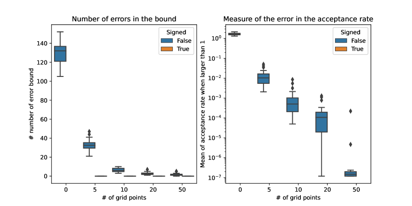
Figure 7: Measure of the errors in the Boomerang sampler for the mixture of Gaussian distributions depending on the grid size and the bounding strategy. The left plot shows the number of times the acceptance rate is larger than $1$, in log scale. The right plot shows the mean value of the acceptance rate when it is larger than $1$, minus $1$, in log scale.

5.3 High dimensional setting

Finally, we consider a high dimensional setting. The target is the banana distribution for the first two dimensions, and a Gaussian distribution for the other dimensions. The potential is defined as $U(x)=\frac{1}{2}x_{1}^{2}+(x_{2}-x_{1}^{2}+1)^{2}+\sum_{i=3}^{d}x_{i}^{2}$. We run a Forward Event Chain algorithm [19] using the Forward Ref version, with the slight modification that the orthogonal rotation is done with probability $0.1$ at each event, instead of the deterministic schedule, no refresh rate $\bar{\lambda}=0$. The horizon $t_{\textnormal{max}}$ is again set to be adaptive with $\alpha_{+}=1.01$ and $\alpha_{-}=1.04$. The process is run for $1$M skeleton points, with $20$ different runs for each combination of $N\in\{0,3,5,10,20\}$ and the bounding strategy (except for $N=0$ where only the no signed strategy is used).

As the target is not multimodal, the errors in the upper bound are low : a mean $0.2$ of errors per chain for $N=0$ (Brent’s algorithm) and $0.05$ for $N=3$ and the no signed strategy. For all the other cases, there is no error in the upper bound. We present in table 1 several quantities of interest for the different strategies and grid sizes. All of them are the mean of the $20$ runs. We show the running time of the algorithm in seconds, the average value of $t_{\textnormal{max}}$, the mean acceptance rate for the thinning, the number of rejections and the number of times the horizon is reached without any event, corresponding to line 1 of algorithm 4.

In this case, as the potential is almost convex, the strategies show very similar results. However, it illustrates the general behavior of the algorithm depending on the number of grid points $N$ . The more grid points, the more accurate the upper bound (higher thinning acceptance rate and lower number of rejections). The fewer rejections, the less $t_{\textnormal{max}}$ is decreased during the process. Therefore, $t_{\textnormal{max}}$ increases, resulting in a lower number of times the horizon is reached without any event. As discussed in section 3.4, the ratio of the adaptation parameters $\frac{\alpha_{+}-1}{\alpha_{-}-1}$, here $.25$, is connected to the ratio between the number of time the horizon is reached and the number of events that are rejected.

N	signed	time	mean $t_{\textnormal{max}}$	thinning AR	# rejection	# hitting horizon
0	False	35.9	0.75	0.734	6.09e+05	2.76e+06
3	False	6.75	1.06	0.789	4.05e+05	1.81e+06
3	True	6.72	1.06	0.789	4.05e+05	1.81e+06
5	False	6.97	1.46	0.838	2.67e+05	1.17e+06
5	True	6.79	1.46	0.838	2.67e+05	1.17e+06
10	False	7.82	2.05	0.889	1.59e+05	6.90e+05
10	True	7.61	2.05	0.889	1.59e+05	6.90e+05
20	False	9.37	2.62	0.927	9.38e+04	4.01e+05
20	True	9.21	2.62	0.927	9.38e+04	4.01e+05

Table 1: Results for several quantities of interest in the high dimension setting

6 Conclusion

Starting from the automatic Zig-Zag algorithm [11] , we have proposed a new method to compute an upper bound of the rate function of a PDMP. This method is based on a grid of the time space, and create a piecewise constant bound. We have shown that this upper bound is a correct upper bound of the rate function under some conditions, that depends on the critical points of the rate function and the length between points of the grid. Also, we modified the algorithm to get an automatic adaptation of the horizon $t_{\textnormal{max}}$. We used the method on different PDMP samplers, and showed that it is more efficient than the automatic Zig-Zag algorithm in terms of errors in the upper bound, and in terms of computation time. Finally, the library is made to be easily used and the definition of a new PDMP can be done in a few lines of code. Further work could be done to create a more efficient adaptation of the horizon $t_{\textnormal{max}}$, in particular for targets with a complex geometry and advanced PDMPs that incorporate geometric information.

References

- [1] Etienne P. Bernard, Werner Krauth and David B. Wilson “Event-Chain Monte Carlo Algorithms for Hard-Sphere Systems” In Physical Review E 80.5 American Physical Society, 2009, pp. 056704 DOI: 10.1103/PhysRevE.80.056704
- [2] Andrea Bertazzi, Joris Bierkens and Paul Dobson “Approximations of Piecewise Deterministic Markov Processes and Their Convergence Properties” In Stochastic Processes and their Applications 154, 2022, pp. 91–153 DOI: 10.1016/j.spa.2022.09.004
- [3] Joris Bierkens “Non-Reversible Metropolis-Hastings” In Statistics and Computing 26.6, 2016, pp. 1213–1228 DOI: 10.1007/s11222-015-9598-x
- [4] Joris Bierkens, Paul Fearnhead and Gareth Roberts “The Zig-Zag Process and Super-Efficient Sampling for Bayesian Analysis of Big Data” In The Annals of Statistics 47.3 Institute of Mathematical Statistics, 2019, pp. 1288–1320 DOI: 10.1214/18-AOS1715
- [5] Joris Bierkens and Gareth Roberts “A Piecewise Deterministic Scaling Limit of Lifted Metropolis–Hastings in the Curie–Weiss Model” In The Annals of Applied Probability 27.2 Institute of Mathematical Statistics, 2017, pp. 846–882 DOI: 10.1214/16-AAP1217
- [6] Joris Bierkens, Gareth O. Roberts and Pierre-André Zitt “Ergodicity of the zigzag process” In The Annals of Applied Probability 29.4 Institute of Mathematical Statistics, 2019, pp. 2266 –2301 DOI: 10.1214/18-AAP1453
- [7] Joris Bierkens, Sebastiano Grazzi, Kengo Kamatani and Gareth Roberts “The Boomerang Sampler” In Proceedings of the 37th International Conference on Machine Learning PMLR, 2020, pp. 908–918
- [8] Alexandre Bouchard-Côté, Sebastian J. Vollmer and Arnaud Doucet “The Bouncy Particle Sampler: A Nonreversible Rejection-Free Markov Chain Monte Carlo Method” In Journal of the American Statistical Association 113.522, 2018, pp. 855–867 DOI: 10.1080/01621459.2017.1294075
- [9] James Bradbury et al. “JAX: composable transformations of Python+NumPy programs”, 2018 URL: http://github.com/google/jax
- [10] Fang Chen, László Lovász and Igor Pak “Lifting Markov Chains to Speed up Mixing” In Proceedings of the Thirty-First Annual ACM Symposium on Theory of Computing Atlanta Georgia USA: ACM, 1999, pp. 275–281 DOI: 10.1145/301250.301315
- [11] Alice Corbella, Simon E. F. Spencer and Gareth O. Roberts “Automatic Zig-Zag Sampling in Practice” In Statistics and Computing 32.6, 2022, pp. 107 DOI: 10.1007/s11222-022-10142-x
- [12] M. H. A. Davis “Piecewise-Deterministic Markov Processes: A General Class of Non-Diffusion Stochastic Models” In Journal of the Royal Statistical Society: Series B (Methodological) 46.3 John Wiley & Sons, Ltd, 1984, pp. 353–376 DOI: 10.1111/j.2517-6161.1984.tb01308.x
- [13] Mark H. A. Davis “Markov Models and Optimization”, Monographs on Statistics and Applied Probability 49 London: Chapman & Hall, 1993
- [14] Persi Diaconis, Susan Holmes and Radford M. Neal “Analysis of a Nonreversible Markov Chain Sampler” In The Annals of Applied Probability 10.3 Institute of Mathematical Statistics, 2000, pp. 726–752 JSTOR: 2667319
- [15] Paul Gustafson “A guided walk Metropolis algorithm” In Statistics and Computing 8.4, 1998, pp. 357–364 DOI: 10.1023/A:1008880707168
- [16] Alan M. Horowitz “A generalized guided Monte Carlo algorithm” In Physics Letters B 268.2, 1991, pp. 247 –252 DOI: https://doi.org/10.1016/0370-2693(91)90812-5
- [17] Kengo Kamatani and Xiaolin Song “Non-reversible guided Metropolis kernel” In Journal of Applied Probability 60.3, 2023, pp. 955–981 DOI: 10.1017/jpr.2022.109
- [18] P. a. W Lewis and G. S. Shedler “Simulation of Nonhomogeneous Poisson Processes by Thinning” In Naval Research Logistics Quarterly 26.3, 1979, pp. 403–413 DOI: 10.1002/nav.3800260304
- [19] Manon Michel, Alain Durmus and Stéphane Sénécal “Forward Event-Chain Monte Carlo: Fast Sampling by Randomness Control in Irreversible Markov Chains” In Journal of Computational and Graphical Statistics 29.4, 2020, pp. 689–702 DOI: 10.1080/10618600.2020.1750417
- [20] Manon Michel, Sebastian C. Kapfer and Werner Krauth “Generalized Event-Chain Monte Carlo: Constructing Rejection-Free Global-Balance Algorithms from Infinitesimal Steps” In The Journal of Chemical Physics 140.5, 2014, pp. 054116 DOI: 10.1063/1.4863991
- [21] Filippo Pagani et al. “NuZZ: Numerical Zig-Zag for General Models” In Statistics and Computing 34.1, 2024, pp. 61 DOI: 10.1007/s11222-023-10363-8
- [22] E. A. J. F. Peters and G. With “Rejection-free Monte Carlo sampling for general potentials” In Physical Review E 85.2 Eindhoven, The Netherlands: APS, 2012, pp. 026703
- [23] Matthew Sutton and Paul Fearnhead “Concave-Convex PDMP-based Sampling” In Journal of Computational and Graphical Statistics 32.4 Taylor & Francis, 2023, pp. 1425–1435 DOI: 10.1080/10618600.2023.2203735
- [24] Paul Vanetti, Alexandre Bouchard-Côté, George Deligiannidis and Arnaud Doucet “Piecewise-Deterministic Markov Chain Monte Carlo” arXiv, 2018 arXiv:1707.05296 [stat]
- [25] Giorgos Vasdekis and Gareth O. Roberts “Speed Up Zig-Zag” arXiv, 2022 arXiv:2103.16620 [math, stat]
- [26] Changye Wu and Christian P. Robert “Coordinate Sampler: A Non-Reversible Gibbs-like MCMC Sampler” In Statistics and Computing 30.3, 2020, pp. 721–730 DOI: 10.1007/s11222-019-09913-w
- [27] Changye Wu and Christian P. Robert “Generalized Bouncy Particle Sampler”, 2017, pp. 1–28 URL: http://arxiv.org/abs/1706.04781