Thermodynamics of the Fermi gas in a cubic cavity of an arbitrary volume
Abstract
For the Fermi gas filling the space inside a cubic cavity of a fixed
volume, at arbitrary temperatures and number of particles, the
thermodynamic characteristics are calculated, namely: entropy,
thermodynamic potential, energy, pressure, heat capacities and
thermodynamic coefficients. The discrete structure of energy levels
is taken into account and size effects at low temperatures are
studied. The transition to the continual limit is considered.
Key words: Fermi particle, electron, volume, thermodynamic functions,
low-dimensional systems, equation of state, heat capacity,
compressibility
pacs:
64.10.+h, 64.60.an, 67.10.Db, 67.30.ej, 73.21.– bI Introduction
The ideal Fermi gas model is the basis for understanding the properties of metals, electron and other multifermion systems. In many cases, it is possible to describe with acceptable accuracy also the behavior of systems of interacting Fermi particles in the framework of the approximation of an ideal gas of quasiparticles, whose dispersion law differs from the dispersion law of free particles. It is essential that all thermodynamic characteristics of ideal Fermi gas at arbitrary temperatures in the case of a large volume can be expressed through the special Fermi-Stoner functions and, thus, all relations of phenomenological thermodynamics can be obtained and checked in the framework of the quantum microscopic model.
Currently, much attention is paid to the study of quantum properties of systems with a small number of particles, such as quantum dots, other mesoscopic objects and nanostructures. In this connection, the problem of description of such objects with taking into account their interaction with the external environment is actual.
Statistical description is usually used to study systems with a very large number of particles. But statistical methods of description can also be applied in the study of equilibrium states of systems with a small number of particles and even a single particle. When considering a system within a large canonical ensemble, it is assumed that it is a part of a very large system, a thermostat, with which it can exchange energy and particles. The thermostat itself is characterized by such statistical quantities as temperature and chemical potential . Assuming that the subsystem under consideration is in thermodynamic equilibrium with the thermostat, the subsystem itself, even consisting of a small number of particles, will be characterized by the same quantities. For example, we can consider the thermodynamics of an individual quantum oscillator LL . In the case when an exchange of particles with a thermostat is possible, the time-averaged number of particles of a small subsystem may be not an integer and, in particular, even less than unity.
In statistical physics, entropy and distribution functions of particles over quantum states are calculated under the assumption that the number of particles is very large. Such consideration for fermions leads to the Fermi-Dirac distribution, and for bosons – to the Bose-Einstein distribution LL . In work PS , the authors calculated the entropy and distribution functions of non-interacting particles in the case when no restrictions are imposed on their number in a system being in thermodynamic equilibrium with the environment. In PS2 , the thermodynamic properties of a two-level system of finite volume were studied in detail.
The influence of boundaries on the behavior of heat capacity in metal colloids has been theoretically studied by Fröhlich long ago Fr . Currently, the experimental possibilities for studying low-dimensional systems at low temperatures are much wider, so that there is an urgent need for a systematic, more detailed theoretical study of such systems. Thermodynamic functions for the Fermi gas confined between two planes and in a cylindrical tube were previously calculated by the authors in PS3 ; PS4 .
In this work, for the Fermi gas filling the space inside a cubic cavity of a fixed volume, at arbitrary temperatures and number of particles, taking into account the results of PS ; PS2 , we calculate its thermodynamic characteristics, namely: entropy, thermodynamic potential, energy, pressure, heat capacities and thermodynamic coefficients. At low temperatures, the discrete structure of energy levels is taken into account and size effects are studied. The transition to the continual limit in the limit of large volume and high temperatures is considered.
II States of Fermi particles in a cubic cavity
Let us consider the thermodynamic properties of the Fermi gas enclosed in a cubic cavity with side and volume . No restrictions are imposed on the side length of the cube, and, therefore, the approach used is applicable to the study of small-sized objects containing a small number of particles. Preliminarily we consider the classification of states of one particle, assuming that its spin is equal to 1/2 and the potential barrier on the surface of the cube is infinite, so that the wave function of a particle at the boundaries turns to zero. Then its normalized wave function has the form
| (1) |
Wave numbers are determined by formula , and integer numbers run through the values Thus, each state is characterized by a set of integers , which for brevity we will sometimes denote by a single symbol . The energy in state
| (2) |
depends only on the combination of integers
| (3) |
so that the states are degenerate. Let us number the energy by index in the ascending order . Also denote by the multiplicity of degeneracy of a level, taking into account the two-fold degeneracy in the spin projection in the absence of a magnetic field. Thus, the summation over states is equivalent to the summation over index with taking into account the multiplicity of degeneracy: . The bottom ten states by the energy and the multiplicity of their degeneracy are given in Table I.
| 1 | 2 | 3 | 4 | 5 | 6 | 7 | 8 | 9 | 10 | |
| 3 | 6 | 9 | 11 | 12 | 14 | 17 | 18 | 19 | 21 | |
| 16 | 48 | 48 | 48 | 16 | 96 | 48 | 48 | 48 | 96 |
– the level number in the order of increasing energy; ,
– the degeneracy factor of a level with account of two-fold degeneracy in the spin projection.
III Distribution function for arbitrary number of particles
Equations for the populations of levels for an arbitrary and even small number of particles were obtained by the authors in PS ; PS2 . We reproduce here briefly these results for fermions. When constructing the thermodynamics of a system with an arbitrary number of particles and an arbitrary size, we will proceed from a combinatorial expression for entropy. If at each level of a quantum Fermi system with the energy and degeneracy factor there are particles, then the statistical weight of such a state is given by the formula LL
| (4) |
The entropy is defined as the logarithm of the total statistical weight by the relation
| (5) |
To calculate all factorials for , the Stirling formula is usually used in the form
| (6) |
For small the accuracy of this formula is insufficient. So, for example, with its accuracy is 7.5%. For there are negative numbers on the right in (6). If, as it is assumed, the time-averaged number of particles can be arbitrary, in particular small and fractional, the factorial should be defined through the gamma function AS :
| (7) |
In this case, the statistical weight (4) is also expressed through the gamma function:
| (8) |
This implies the formula for nonequilibrium entropy :
| (9) |
If a level is filled or empty , then it does not contribute to the total entropy. Taking into account that the total number of particles and the total energy are determined by the formulas
| (10) |
| (11) |
the average number of particles at level , or the population of the level, is found from the condition
| (12) |
where are the Lagrange multipliers. From this condition we find the equation that determines the average number of particles in each state PS ; PS2 at :
| (13) |
where is the logarithmic derivative of the gamma function (the psi function) AS . From comparison with thermodynamic relations it follows that , , – temperature, – chemical potential. Using the asymptotic formula , which is valid for , we obtain
| (14) |
where
| (15) |
is the usual Fermi-Dirac distribution. Formula (14) gives a good approximation if is not close to zero or unity, and turns into the usual distribution (15) in the limit . It is important to note, however, that the exact function defined by equation (13), in contrast to (15), becomes zero or unity at finite values of energy.
IV Thermodynamic functions, heat capacity, thermodynamic coefficients
The equilibrium entropy, number of particles and energy are determined by formulas (9), (10), (11), taking into account that the average number of particles at a given level as a function of temperature and chemical potential is determined by equation (13). The differential of the thermodynamic potential has the usual form
| (16) |
The pressure
| (17) |
is determined by the dependence of a particle’s energy on volume. In the case under consideration , so that . To calculate heat capacities and thermodynamic coefficients, we first find the differentials of the distribution function, number of particles, entropy and pressure:
| (18) |
| (19) |
| (20) |
| (21) |
Here
| (22) |
where is the trigamma function AS .
In the following we will consider systems with a fixed average number of particles, for which . This condition allows to eliminate the differential of chemical potential and, as a result, the entropy and pressure differentials will take the form
| (23) |
where
| (24) |
In our case , . From these relations there follow the formulas for the isochoric
| (25) |
and the isobaric
| (26) |
heat capacities. We also present following from (23), (24) formulas for the coefficient of volumetric expansion
| (27) |
the isothermal compressibility
| (28) |
and the isochoric thermal pressure coefficient
| (29) |
All other thermodynamic coefficients can be expressed through the heat capacities and the coefficients given here RR . Obviously, the general relation LL
| (30) |
is fulfilled, which confirms the consistency of the given general thermodynamic relations. Since the thermodynamic inequalities and must be satisfied in a stable system LL , then there must be and .
V Low temperatures. Size effects
The most interesting is the case when there are a small number of particles in the volume of a cube of small size. In this case, the discrete structure of the spectrum turns out to be important, so that the exact formulas (9) – (11), (13), (17), (25) – (29) should be used for calculations. Thermodynamic properties of such a system of particles with two discrete levels are considered in detail by the authors in PS2 . In the following, along with dimensional quantities, we will use the writing of quantities in dimensionless form, introducing arbitrary characteristic scales of length , energy and pressure . Note that . For example, the Bohr radius cm or some other length can be chosen as the spatial scale. The dimensionless length , temperature , pressure and level energy are defined by the relations:
| (31) |
Let us estimate the temperature and the cube size, at which the size effects become significant. Obviously, these effects will manifest themselves when the temperature becomes comparable to the energy difference between levels, which is of the order of the energy of the ground level. Its energy can be represented in the form
| (32) |
where cm, eV K is the Rydberg unit. The size, at which K is equal to or cm. Thus, at temperature of the order of one Kelvin the size effects should manifest themselves already in samples of macroscopic dimensions.
Let us first consider the state of the system at zero temperature. If the number of particles is less than or equal to the degeneracy factor of the first level , then , and the particles are only at the ground level. Higher levels are not filled. In this case the population of the first level is determined by the relation , and the energy, pressure and thermodynamic coefficients are equal to , , , , . The entropy
| (33) |
turns to zero only for the fully occupied level and is different from zero for the unfilled level. In this case, the third law of thermodynamics is satisfied in the Nernst formulation, while in the Planck formulation it is satisfied only at fully occupied levels.
If lower levels are completely filled, and the level can be partially filled, then and , and the chemical potential . In this case, the entropy is given by formula (33) with the substitution , and the total number of particles, energy, pressure and thermodynamic coefficients are determined by formulas , , , , , . The size effect, which manifest itself in discreteness of levels, leads to the situation that near zero temperature there is a temperature region in which the populations of levels do not change with temperature and remain the same as at .
In the temperature region where the temperature dependence of populations arises, the quantities (24) through which the heat capacities and thermodynamic coefficients (25) – (30) are expressed, can be represented in dimensionless variables in the form
| (34) |
where the notation is used
| (35) |
Note that the quantity does not explicitly contain the chemical potential and is positive due to the requirement of thermodynamic stability. The coefficient in a thermodynamically stable system must be negative . It entails the necessity of fulfillment of the inequality , where
| (36) |
At the excited system is unstable, and so the system continues to remain in the same ground state as at . Thus, the calculation of the temperature dependence of any thermodynamic quantity is reduced to the calculation of sums (35). In particular, the pressure (17) is
| (37) |
As noted, we consider systems in which the time-averaged number of particles can vary within range . As will be seen, there is some critical value , so that the cases and should be considered separately. Let us first consider the case , assuming that the number of particles is less than or equal to the degeneracy factor of the first level . In this case, particles will begin to transit from the ground to the second level at the temperature
| (38) |
In case of fulfillment of the conditions and , the stability condition is satisfied. At the critical value of the coefficient turns to zero already at the temperature , and at it proves to be positive. Therefore, the case will be considered separately below.
Here and further we use the notation
| (39) |
The functions are defined in (13), (22), and
| (40) |
where . In the considered case the inequality is fulfilled, so as noted above the stability condition at is satisfied. Obviously, the existence of characteristic temperatures (36), (38) is caused by the finite size of the system and they tend to zero at . At temperature slightly above (38) we have
| (41) |
Taking this into account we conclude that the quantities are continuous at , and the heat capacities and thermodynamic coefficients undergo jumps here:
| (42) |
where , and , et al.
Let us consider the behavior of thermodynamic quantities near and above the temperature (38), assuming , where . Here the continuous transition of particles from the ground to the second level begins. Then the populations of levels are , , and also . From the condition of conservation of the total number of particles it follows that . The dependence of populations on temperature is found from the system of equations
| (43) |
where . As a result, near and above we have
| (44) |
| (45) |
| (46) |
From (44) – (46) and relations (9), (25) – (29), (37) it follows that near and above the thermodynamic quantities depend linearly on temperature:
| (47) |
The coefficient , which determines the slope of the line, for different quantities is given by the formulas:
| (48) |
Here , and the values of thermodynamic quantities at temperature are determined by the formulas:
| (49) |
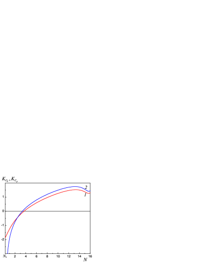
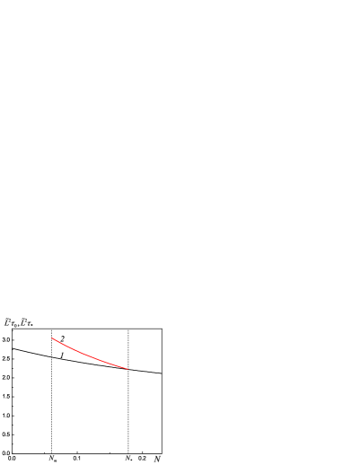
The coefficients (48) and their sign depend on the number of particles. The coefficients and are positive for all . The dependences of the coefficients and on the number of particles are shown in Fig. 1. The coefficient at has a finite negative value , and at it changes sign. The coefficient tends to an infinite negative value at and changes sign at .
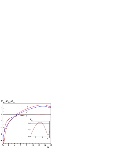
The dependences of the coefficients , and on the number of particles are shown in Fig. 2. They are qualitatively similar to those shown in Fig. 1. The coefficient at takes on a finite negative value and changes sign at . The coefficients and tend to an infinite negative value at . The coefficient changes sign at , and turns to zero at the points . All curves in figures 1 and 2 have minima at near .
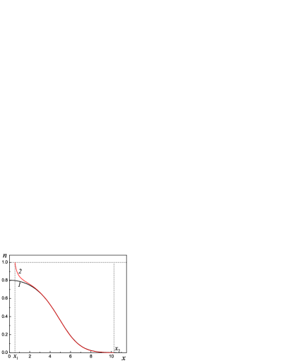
With a further increase in temperature there occur transitions of particles not only to the second, but also to higher levels, so that the temperature dependences of the quantities become more complex. As an illustration, Fig. 3 shows the calculation of the temperature dependences of populations of levels up to a temperature close to the energy of the fourth level for under the assumption . At temperature the transition of particles from the first to the second level begins, at the third and fourth levels begin to populate with particles, respectively.
At , where , there is a characteristic temperature at which the probability of filling of the first level turns to zero. At the temperature , with . At the temperature is absent, and some fraction of particles continues to remain at the ground level at all temperatures.
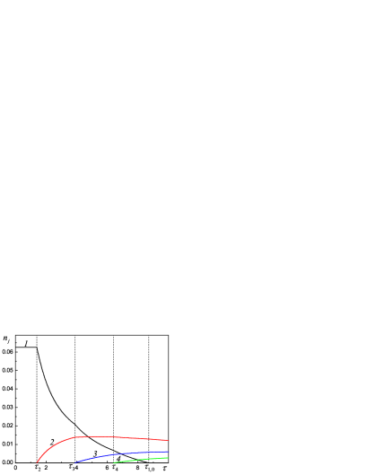
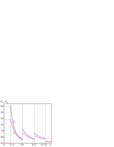
Figure 4 shows the dependences of heat capacities and on temperature under the same conditions as in Fig. 3. The heat capacities undergo jumps at temperatures at which the filling of new levels begins, or when the population of the ground level turns to zero.
The developed approach allows to consider systems in which the time-averaged number of particles, due to the exchange of particles with the thermostat, can be non-integer, and, in particular, less than unity. As noted above, the case should be considered separately, because in this case the system at is unstable due to the inequality . In this case to be considered now, the system remains in the ground state up to the temperature . When going above this temperature, a redistribution of particles between two levels to the values and occurs by a jump.
In what follows we will use notations similar to (39):
| (50) |
and also . From (36), taking into account that , and , it follows that the temperature is determined by the equation
| (51) |
and besides . The last relation is fulfilled if we introduce the angle , such that , . From equations (43) we find
| (52) |
By eliminating from (51) and (52), we obtain the equation that allows to find the populations and at :
| (53) |
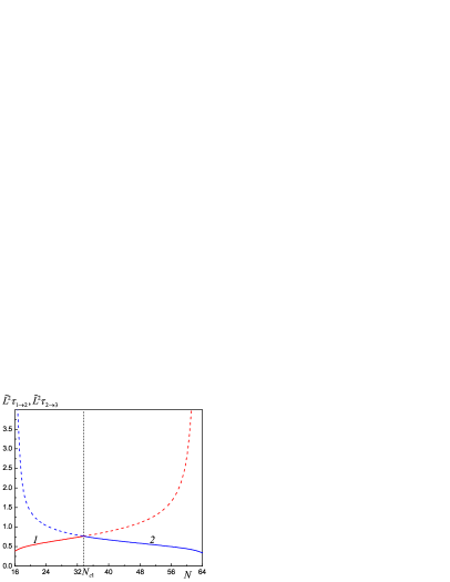
Knowing the populations, from (51) or (52) we find the critical temperature . The calculation for gives , , . Equation (53) has a solution in the range of the number of particles . Here , to which corresponds , , , and , to which corresponds , , . The dependencies of the temperatures and on the number of particles are shown in Fig. 5.
At temperature the energy, pressure, entropy, isochoric heat capacity and isochoric thermal pressure coefficient undergo a jump
| (54) |
Due to the fact that at the coefficient , the isobaric heat capacity tends to infinity
| (55) |
where . The heat capacity goes to infinity due to the fact that the interaction between particles is neglected. Taking into account such interaction should lead to a finite value of the heat capacity at . This situation is qualitatively similar to that which occurs in the boson gas near the condensation temperature YP ; YP2 . The coefficient of volumetric expansion and the coefficient of isothermal compressibility have similar singularities:
| (56) |
For an even smaller number of particles the coefficient is always positive, so that the stability condition for excited states is not satisfied, and the system is in the ground state at any temperature. A similar possibility was considered earlier by the authors in the two-level system PS2 .
In the same way as is done for the case , the temperature dependences of the populations and thermodynamic characteristics can be analyzed for the case when at zero temperature lower levels are completely filled and the level can be filled partially. For definiteness, we briefly consider the case when . Here at the first level is completely filled with , and on the second level there are particles, so that . The third and higher levels are empty. In this case, there are two possibilities of transition of the system to the excited state. At the temperature
| (57) |
the transition from the first level to the second level begins, while the third level remains empty. A case is possible, when the system is excited as a result of transition of particles from the second to the third level with the ground level being completely filled. This occurs at the temperature
| (58) |
In fact, the excitation of the system will begin at that of the temperatures (57), (58) which proves to be lower for a given number of particles. The dependence of these temperatures on the number of particles is shown in Fig. 6.
VI Continual approximation
If particles in a gas interact through short-range forces with interaction radius , then the ideal gas approximation can be used if the volume per one particle is much larger than the volume of an atom , or . For a large system, the volume of which is much larger than the volume per one particle , the condition must be satisfied; however, it is necessary that . In this approximation, the extensive quantities are proportional to the volume. In statistical mechanics, it is common to go to the thermodynamic limit and at . In the problem under consideration, the effects caused by the finite volume of the system are investigated. Let us consider in more detail the transition to the continual approximation at a large volume, when such effects are small.
Since in the number space there is a cube of unit volume per one such state, then the total number of states in a large system, for which the condition is satisfied and whose energy is less than , is equal to the volume of the sphere
| (59) |
The number of states in the interval is , so that the density of the number of states on the surface of a sphere of radius is equal to the surface area of this sphere
| (60) |
The degeneracy factor of the level with energy with account of the two-fold degeneracy in the spin projection is
| (61) |
Let us proceed to the description of the system in the continual approximation. First assume that the number of levels is finite and denote . Then the total number of particles
| (62) |
Further divide the interval of change of into equal intervals . Given the definition of the de Broglie thermal wavelength
| (63) |
let us introduce dimensionless quantities , and . Then formula (62) will take the form
| (64) |
Let us consider the limiting case . In the limit this condition is true at any temperature. In the case of a finite volume system we are interested in, this condition is satisfied if or . Thus, at a finite volume, one can move on to a continual description at high temperatures when the de Broglie thermal wavelength is much smaller than the cube’s edge length. Considering and passing from summation to integration in (64), we obtain
| (65) |
Similarly, the transition to the continual approximation can be performed for other thermodynamic quantities.
The equation that determines the average number of particles in each state (13) can be written in the form
| (66) |
where . In the continual approximation can be considered as a continuous variable, and according to formula (61)
| (67) |
In this case, the quantities (35) take the form
| (68) |
where
| (69) |
If the conditions and are fulfilled, then the distribution function turns into the usual Fermi-Dirac distribution
| (70) |
Figure 7 shows the distribution function in the continual approximation and the Fermi-Dirac function . In the main region of variation of the wave number these functions are very close. The fundamental difference between them is that is different from zero and unity in the entire region , while varies in the finite region , and furthermore at it turns to unity and at to zero.
In the continual approximation, using the Fermi-Dirac distribution (70), all thermodynamic quantities can be expressed through the standard functions introduced by Stoner DS :
| (71) |
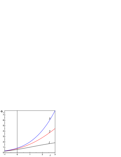
where is the gamma function, . As a rule, it is sufficient to use functions with indices , for which . A view of these functions is shown in Fig. 8. Let us give expressions through functions (71) for the thermodynamic potential, number of particles, pressure, energy and entropy of the Fermi gas in a large volume without taking into account boundary effects:
| (72) |
where , . Through the same functions one can express the heat capacities
| (73) |
and the thermodynamic coefficients
| (74) |
Using asymptotic formulas, one can obtain thermodynamic relations in the limiting cases of high and low temperatures. In the high-temperature limit and , there holds the asymptotics . Another limiting case corresponds to the case of a quantum gas close to degeneracy at low temperatures. Here, with accuracy up to exponentially small terms, we have the formulas
| (75) |
The given formulas are valid both in the limit of infinite volume and for a system of finite dimensions provided the condition is fulfilled.
VII Conclusion
In the presented work, we construct the thermodynamics and calculate the energy, pressure, entropy, heat capacities and thermodynamic coefficients of the Fermi gas enclosed in a cubic cavity of finite volume. It is assumed that the average number of particles in a volume can be arbitrary, in particular small and fractional. It is taken into account that the form of the distribution function, as previously shown by the authors PS ; PS2 , differs from the standard Fermi-Dirac function. The main feature of the exact distribution function is that it does not have ”exponential tails”, but turns to zero or unity at finite energy. The case of low temperatures is considered, when the discrete structure of the energy spectrum arising due to the size effect becomes important. It is shown that the excitation of the system begins at some finite temperature. Below this temperature the system continues to remain in the same state as at zero temperature. It is characteristic that if there is a not completely occupied level in the system, then the entropy remains different from zero at zero temperature, so that the third law of thermodynamics proves to be fulfilled only in the Nernst formulation. As each new level begins filling, there happens a jump in heat capacities. The transition to the continual approximation is considered, which becomes possible if the de Broglie thermal wavelength turns out to be much smaller than the cube’s edge length. In this limit, if the Fermi-Dirac function is used as the distribution function, all thermodynamic quantities can be expressed through the standard Fermi-Stoner functions.
References
- (1) L.D. Landau, E.M. Lifshitz, Statistical physics: Vol. 5 (Part 1), Butterworth-Heinemann, 544 p. (1980).
- (2) Yu.M. Poluektov and A.A. Soroka, Quantum distribution functions in systems with an arbitrary number of particles (2023). arXiv:2311.03003 [quant-ph]
- (3) Yu.M. Poluektov and A.A. Soroka, On the thermodynamics of two-level Fermi and Bose nanosystems, Opt. Quant. Electron. 56, 1349 (2024). doi:10.1007/s11082-024-07266-x; arXiv:2405.02427 [quant-ph]
- (4) H. Fröhlich, The specific heat of electrons in small metal particles at low temperatures, Physica 4, 406 – 412 (1937). doi:10.1016/S0031-8914(37)80143-3
- (5) Yu.M. Poluektov and A.A. Soroka, Thermodynamics of the Fermi gas in a quantum well, East Eur. J. Phys. 3, №4, 4 – 21 (2016). arXiv:1608.07205 [cond-mat.stat-mech]
- (6) Yu.M. Poluektov and A.A. Soroka, Thermodynamics of the Fermi gas in a nanotube, East Eur. J. Phys. 4, №3, 4 – 17 (2017). arXiv:1704.03317 [physics.gen-ph]
- (7) M. Abramowitz, I. Stegun (Editors), Handbook of mathematical functions, National Bureau of Standards Applied mathematics Series 55, 1046 p. (1964).
- (8) Yu.B. Rumer, M.S. Ryvkin, Thermodynamics, statistical physics, and kinetics, Mir publishers, Moscow, 600 p. (1980).
- (9) J. McDougall, E.C. Stoner, The computation of Fermi-Dirac functions, Phil. Trans. Roy. Soc. A 237, 67 – 104 (1938). doi:10.1098/rsta.1938.0004
- (10) Yu.M. Poluektov, Isobaric heat capacity of an ideal Bose gas, Russ. Phys. J. 44 (6), 627 – 630 (2001). doi:10.1023/A:1012599929812
- (11) Yu.M. Poluektov, A simple model of Bose-Einstein condensation of interacting particles, J. Low Temp. Phys. 186, 347 – 362 (2017). doi:10.1007/s10909-016-1715-5