Self-tuning moving horizon estimation of nonlinear systems via physics-informed machine learning Koopman modeling

Abstract

In this paper, we propose a physics-informed learning-based Koopman modeling approach and present a Koopman-based self-tuning moving horizon estimation design for a class of nonlinear systems. Specifically, we train Koopman operators and two neural networks - the state lifting network and the noise characterization network - using both data and available physical information. The two neural networks account for the nonlinear lifting functions for Koopman modeling and describing system noise distributions, respectively. Accordingly, a stochastic linear Koopman model is established in the lifted space to forecast the dynamic behavior of the nonlinear system. Based on the Koopman model, a self-tuning linear moving horizon estimation (MHE) scheme is developed. The weighting matrices of the MHE design are updated using the pre-trained noise characterization network at each sampling instant. The proposed estimation scheme is computationally efficient because only convex optimization is involved during online implementation, and updating the weighting matrices of the MHE scheme does not require re-training the neural networks. We verify the effectiveness and evaluate the performance of the proposed method via the application to a simulated chemical process.

Keywords: Nonlinear process, Physics-informed machine learning, Koopman operator, Moving horizon estimation.

1 Introduction

Koopman operator-based data-driven modeling and model predictive control (MPC) has become an emerging integrated modeling and optimal control framework for nonlinear systems, particularly in cases where high-fidelity mechanistic models are absent or accurate model parameters are unavailable. According to Koopman theory, for any nonlinear system, it is possible to find a higher-dimensional space where a Koopman operator can be identified to describe the dynamic evolution of the original nonlinear system in a linear manner [1, 2]. Within a Koopman operator framework, linear MPC strategies can be proposed and applied for nonlinear systems, and complex and time-consuming nonlinear optimization associated with conventional nonlinear MPC methods can be bypassed.

A variety of Koopman-based MPC algorithms have been developed. In [3, 4, 5], Koopman operators were used to approximate the dynamics of deterministic nonlinear systems, leading to the development of deterministic linear convex MPC based on the obtained Koopman model. In [6], tube-based MPC was proposed to address nonlinear discrete systems with potential exogenous disturbances and noise, which offers greater tolerance for modeling approximation errors. In [2, 7], various Koopman modeling strategies were employed to establish robust Koopman MPC. Additionally, in [8], a Koopman-based economic MPC scheme was proposed to achieve better economic operational performance. While the Koopman-MPC framework has been well studied, a critical remaining issue is the requirement for full-state measurements for online decision-making in most Koopman-based MPC methods. In real applications, measuring some key variables online using hardware sensors can be challenging [9, 10]. This necessitates state estimation, which provides real-time estimates of the necessary quality variables based on limited output measurements [11, 12, 13, 14, 15, 16, 17]. In this work, we aim to leverage the Koopman operator concept to develop a computationally efficient state estimation method for nonlinear systems, which can be integrated with Koopman MPC for efficient monitoring and optimal operation of general nonlinear systems.

Various data-driven Koopman modeling approaches have been proposed to build models suitable for implementing linear estimation and control algorithms. Extended dynamic mode decomposition (EDMD) [18] is one of the most representative methods. This type of method lifts the system state to a high dimensional space through manually selected lifting functions such as basis functions and reproducing kernels. Then, a least-squares problem is solved to build Koopman operators, and the resulting linear state-space model in the higher-dimensional space can be leveraged for linear estimation and control [18, 19]. However, selecting appropriate lifting functions may require extensive experience and domain knowledge about the underlying dynamics of each specific process [20, 18]. It is also challenging to find suitable lifting functions through manual selection when dealing with large-scale systems [21, 18].

In our recent work [21], we made an initial attempt on Koopman-based constrained state estimation for nonlinear systems using EDMD-based modeling. While promising results were achieved, scaling this approach to systems with numerous state variables remains constrained by the difficulty of manually selecting extensive lifting functions. To address this challenge, learning-based approaches to Koopman modeling have been proposed, where neural networks embed the system state into a lifted space. This type of method automates the selection of lifting functions by training Koopman operators on offline data [22], which holds the promise to facilitate broader adoption of Koopman modeling for nonlinear system estimation and control. However, the effectiveness of learning-based Koopman models heavily relies on the quantity and quality of available data. Achieving accurate approximation and generalization demands diverse and sufficiently large training datasets. Neural networks can struggle with small-scale datasets, leading to overfitting or convergence issues. Moreover, the performance of neural network-based lifting functions and resulting Koopman models can be significantly impacted by noise and outliers in the data [23].

In machine learning, one way to address challenges related to data scarcity and poor data quality is to incorporate available valuable physical knowledge into neural network training, which is known as physics-informed neural networks (PINNs) [24]. PINN-based methods have been widely used for approximating partial differential equations (PDEs) by integrating data and mathematical models to enforce physical laws. PINN has also been considered in addressing control-oriented machine learning modeling for nonlinear ordinary differential equations (ODEs) processes. The use of a PINN-based dynamic model can lead to improved control performance compared with using ODEs and classical integration methods such as fourth-order Runge-Kutta method (RK4)[25, 26, 27]. Physics-Informed Neural Networks (PINNs) hold the promise of being seamlessly integrated with the learning-based Koopman modeling framework, which is particularly relevant for scenarios where data may be scarce for purely data-driven, data-intensive deep learning-based Koopman modeling. By incorporating available physical knowledge into the training process, PINNs can help develop more appropriate neural network-based lifting functions. As discussed previously, purely data-driven models that rely solely on data might fit the training data well. However, the predictions from these models can deviate from real system behaviors due to biases in the collected data, which will lead to poor generalization performance [28]. Incorporating valuable physical information allows neural networks to maintain robustness when conducting machine learning modeling on noisy datasets [24]. Moreover, when data availability is limited, the exploration space of a trained neural network is constrained, and the risk of overfitting is increased. Integrating data and physical information in a unified approach is promising for mitigating overfitting tendencies, resulting in more physically consistent and robust predictions.

Based on the above observations and considerations, in this work, we aim to propose a learning-based Koopman modeling and state estimation approach for general nonlinear systems under practical scenarios where data can be limited and/or noisy. We propose a physics-informed machine learning Koopman modeling approach, which leverages limited data and the available physical knowledge to build a stochastic predictive Koopman model to robustly characterize the dynamics of the considered nonlinear system. A learning-enabled MHE scheme with self-tuning weighting matrices is developed based on the Koopman model. In this scheme, the weighting matrices of the Koopman MHE are updated online using a pre-trained noise characterization network to reduce the efforts of manual parameter tuning associated with conventional MHE designs. This estimation scheme solves a convex optimization problem at each sampling instant to online estimate the state of the underlying nonlinear system efficiently. A benchmark reactor-separator process example is introduced to illustrate the proposed approach. Our method showcases its capability to build an accurate Koopman model using less data than required for purely data-driven Koopman modeling methods. Moreover, the self-tuning of weighting matrices in the MHE leads to more precise state estimates as compared to conventional designs where weighting matrices remain constant.

2 Preliminaries and problem formulation

2.1 Notation

$x_{i:j}$ contains a sequence of values of vector $x$ from time instant $i$ to $j$, $x_{j|k}$ is the information about $x$ for time instant $j$ obtained at time instant $k$. $\left\|x\right\|^{2}$ represents the Euclidean norm of vector $x$. $\left\|x\right\|^{2}_{P}$ is the square of the weighted norm of vector $x$, that is, $\left\|x\right\|^{2}_{P}=x^{\text{T}}Px$. $\text{diag}\left(x^{i}\right)$ represents a diagonal matrix of which the $i$th main diagonal elements are constituted by the $i$ th elements of vector $x$. $\tilde{f}={[f_{i},f_{j}]}^{\text{T}}$ denotes a new vector consisting of the $i$ th and $j$ th elements of $f$. $\mathcal{N}(a,b)$ denotes a Gaussian distribution with mean $a$ and variance $b$. ${\bf{I}}_{n}$ is an identity matrix with $n\times n$ dimensions. $\bf{0}$ denotes a null matrix of appropriate dimensions.

2.2 Koopman operator for controlled systems

Consider a general discrete-time nonlinear system as follows:

$$x_{k+1}=f(x_{k},u_{k})$$ (1)

where $k$ represents the sampling instant; $x\in\mathbb{X}\subseteq\mathbb{R}^{n}$ denotes the system state; $u\in\mathbb{U}\subseteq\mathbb{R}^{r}$ represents the control input.

Based on the Koopman theory for controlled systems, there exists an infinite-dimensional space $\mathcal{G}$, where the dynamics of (1) can be described using a linear model [3]. Specifically, let us consider an augmented state vector $\mathcal{X}$ defined as $\mathcal{X}=\big{[}x_{k}^{\text{T}},u_{k}^{\text{T}}\big{]}^{\text{T}}$. There exists a lifting function $\Psi$ and a Koopman operator $\mathcal{K}$, which are up to infinite dimensions, such that the dynamic behavior of the augmented state vector $\mathcal{X}$ is governed within a lifted space using the following linear Koopman model:

$$\Psi(\mathcal{X}_{k+1})=\mathcal{K}\Psi(\mathcal{X}_{k}).$$ (2)

From a practical viewpoint, finding the exact infinite-dimensional lifting function, denoted by $\Psi$, and Koopman operator $\mathcal{K}$ for nonlinear system (8) can be infeasible. Instead, we can find a finite-dimensional lifting function $\hat{\Psi}$ and establish an approximate Koopman operator, denoted by $\hat{\mathcal{K}}$, within the corresponding finite-dimensional state space, such that:

$$\hat{\Psi}(\mathcal{X}_{k+1})\approx\hat{\mathcal{K}}\hat{\Psi}(\mathcal{X}_{k}).$$ (3)

Because the augmented state vector $\mathcal{X}$ contains state $x$ and input $u$, the vector of observables can be represented with the following ad hoc form:

$$\hat{\Psi}\left(\left[\begin{array}[]{c}x\\ u\\ \end{array}\right]\right)=\left[\begin{array}[]{c}g(x)\\ u\\ \end{array}\right].$$ (4)

Accordingly, the approximate Koopman operator $\hat{\mathcal{K}}$ can be partitioned into four blocks as follows:

$$\hat{\mathcal{K}}=\left[\begin{array}[]{c;{1.5pt/1.5pt}c}A&B\\ \hdashline[2pt/2pt]*&*\end{array}\right].$$ (5)

Since our focus is on establishing a Koopman model for forecasting the future behavior of state $x$ rather than predicting the future behavior of the control input $u$, it is sufficient to build a Koopman model that describes the dynamic behavior of $g(x)$, which contains the future information of stat. Consequently, we only need to reconstruct matrices $A$ and $B$ and build a linear Koopman-based state-space model in the following form:

$$g(x_{k+1})=Ag(x_{k})+Bu_{k}$$ (6)

where $A\in\mathbb{R}^{n_{g}\times n_{g}}$, $B\in\mathbb{R}^{n_{g}\times r}$ are sub-matrices of the finite Koopman operator $\hat{\mathcal{K}}$; $g\in\hat{\mathcal{G}}\subseteq\mathbb{R}^{n_{g}}$ denotes the lifting functions. Further, based on the observable set $g$, we can reconstruct the original state $x$ by using an reconstruction matrix $C$ following:

$$x_{k}=Cg(x_{k}).$$ (7)

The remainder of this paper is organized as follows. In Section 2.3, we formally define the problem. In Section 3, we present the network structure of the proposed physics-informed Koopman modeling algorithm and explain the integration of physical information into Koopman theory. In Section 4, we introduce the design of self-tuning MHE using the pre-trained networks and the Koopman operator. In Section 5, we use a simulated chemical process to evaluate the performance of the proposed algorithm. In Section 6, we conclude the paper.

2.3 Problem statement

Consider a general stochastic discrete-time nonlinear system described by the state-space model as follows:

$$x_{k+1} =f(x_{k},u_{k})+w_{k}$$ (8a)

$$y_{k} =h(x_{k})+v_{k}$$ (8b)

where $k$ represents the sampling instant; $x\in\mathbb{X}\subseteq\mathbb{R}^{n}$ denotes the system state; $u\in\mathbb{U}\subseteq\mathbb{R}^{r}$ is the control input; $y\in\mathbb{Y}\subseteq\mathbb{R}^{m}$ is vector of output measurements; $w\in\mathbb{W}=\{\ w\subseteq\mathbb{R}^{n}~{}\text{s.t.}~{}||w||_{2}\leq w_{\max}\}$ and $v\in\mathbb{V}=\{\ v\subseteq\mathbb{R}^{m}~{}\text{s.t.}~{}||v||_{2}\leq v_{\max}\}$ represent the system disturbances and measurement noise respectively, with $w_{\text{max}}$ and $v_{\text{max}}$ are the supremum of $w$ and $v$, respectively; $f:\mathbb{X}\times\mathbb{U}\to\mathbb{X}$ is a nonlinear vector function that describes the dynamic behavior of $x$, and is typically established through first-principles modeling; $h:\mathbb{X}\to\mathbb{Y}$ is the output measurement function.

In this work, we treat the problem of state estimation of the general nonlinear system in (1), under practical case scenarios when accurate details of the first-principles process model, denoted as $f$, and/or the values of the associated model parameters are only partially available. To address the nonlinear state estimation problem in a computationally efficient manner, we aim to leverage both the system data and available physical knowledge about the expression and the parameter values of $f$, to build a stochastic Koopman-based linear dynamic model to approximate the dynamic behaviors of (1), formulated as follows:

$$z_{k+1} =Az_{k}+Bu_{k}+\mu_{k}$$ (9a)

$$\hat{x}_{k} =Cz_{k}$$ (9b)

$$y_{k} =Dz_{k}$$ (9c)

where $z=g(x)\in\hat{\mathcal{G}}\subseteq\mathbb{R}^{n_{g}}$ represents the lifted state vector in the context of the linear Koopman model; $\mu\subseteq\mathbb{R}^{n_{g}}$ is the disturbance to the lifted state; $A\in\mathbb{R}^{n_{g}\times n_{g}}$, $B\in\mathbb{R}^{n_{g}\times r}$, $C\in\mathbb{R}^{n\times n_{g}}$, and $D\in\mathbb{R}^{m\times n_{g}}$ are system matrices to be established from data.

Then, based on the stochastic Koopman model, a linear moving horizon estimation scheme will be developed for constrained linear estimation of the full state $x$ of (1) in a linear manner, despite the nonlinearity of the underlying system dynamics.

3 Physics-informed learning-based Koopman modeling

3.1 Existing approaches to lifting function selection

An appropriate selection of the lifting functions is critical for building an accurate Koopman model with good predictive capabilities. In the existing literature, various methods have been proposed for obtaining finite-dimensional approximations of the Koopman operator and determining the corresponding lifting functions.

Extended dynamic mode decomposition is a representative approach [18]. Within the EDMD framework, the lifting functions are manually selected. In applications, representative lifting functions can be considered, and the candidates may be included or excluded based on trial-and-error analysis, domain knowledge, and users’ experience. Despite its promise in addressing high nonlinearity, the necessity for manual selection restricts the application of EDMD-based Koopman modeling to medium- to large-scale nonlinear systems. Koopman modeling based on Kalman-Generalized Sparse Identification of Nonlinear Dynamics (Kalman-GSINDy) proposed in  [2] creates a rich library containing a comparatively large number of candidate lifting functions, and a Kalman-based algorithm is executed recursively to select the most relevant lifting functions from a pre-defined rich library to account for the nonlinear mapping. However, the creation of the library containing candidate lifting functions remains a non-trivial task, and there may not exist a generalized library that is applicable to a broad range of nonlinear systems.

The learning-based Koopman modeling framework [29, 30, 31] with data-driven modeling has emerged as a promising solution. With this framework lifting functions can be automatically determined by neural networks trained on batch system data [32]. Specifically, a neural network is established to map the original system state $x$ to a finite-dimensional lifted state space, where Koopman operators can be established via either solving the associated optimization directly [29, 30], or using the least-squares solution [31] as adopted in DMD and EDMD-based Koopman modeling approaches [18, 33].

Compared to the conventional methods using manual and semi-automatic lifting function selection for Koopman modeling, the learning-based approaches enable automatic learning of the lifting functions from data. This eliminates the necessity of manually specifying lifting function candidates or associated coefficients. Thus it reduces the reliance of Koopman modeling on trial-and-error tests and users’ experience and improves the applicability of Koopman modeling to practical systems of medium- to large-scales. Meanwhile, it is worth mentioning that the existing learning-based Koopman modeling approaches are purely data-driven [29, 30, 31]. This presents limitations in the following manner: 1) Effective training of neural networks requires a substantial amount of data to elucidate features effectively [34, 35]. With insufficient data samples, neural network models are subject to the risk of focusing solely on the features present in the training set, which may lead to significant overfitting [28]. This issue is particularly critical for systems with a large number of state variables and when more complex neural networks with numerous layers and training parameters are employed. 2) Noise present in datasets can significantly disrupt feature extraction, which further leads to degraded modeling performance [probabilistic]. 3) Even partial information about $f$ in (1) can contain valuable insights related to the real system dynamics. Integrating this physical information can guide neural networks to prioritize features associated with system behaviors, thereby reducing the influence of noise and outliers. This type of solution generates more robust models that perform well even with small-scale and lower-quality datasets.

Based on the above observations, we aim to propose a data-efficient learning-enabled Koopman modeling method that effectively utilizes both the limited data and the available physical information.

3.2 Proposed Koopman model structure

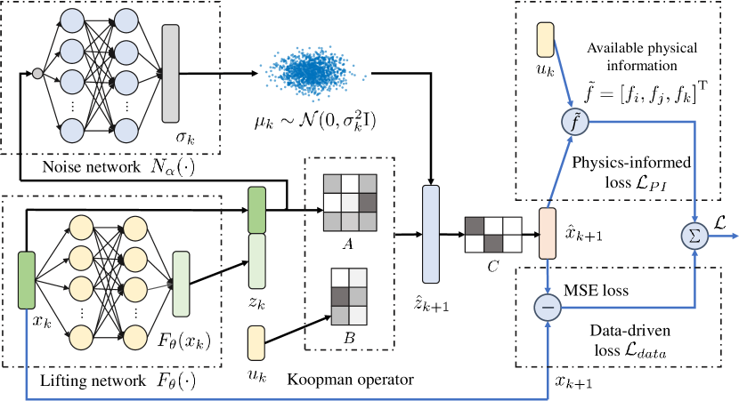
Figure 1: An overview of the proposed Koopman modeling approach.

In this section, we present the structure of the Koopman model. Implementing the proposed physics-informed Koopman modeling approach establishes a state lifting network $F_{\theta}(x)$, a noise characterization network $N_{\alpha}(z)$, and Koopman operators in the form of matrices $A$, $B$, and $C$, as shown in Figure 1. The two neural networks and the Koopman operators are integrated to form a stochastic Koopman model for multiple-step-ahead prediction of state $z$ in the lifted state space. Specifically, the stochastic Koopman model is in the following form:

$$\hat{z}_{k+j+1|k} =A\hat{z}_{k+j|k}+Bu_{k+j}+\mu_{k},\ j=0,\dots,H-1$$ (10a)

$$\hat{x}_{k+j|k} =C\hat{z}_{k+j|k}$$ (10b)

$$y_{k+j|k} =D\hat{z}_{k+j|k}$$ (10c)

where $\hat{z}_{k+j|k}$ is a prediction of $z_{k+j}$ obtained at time instant $k$; $\mu_{k}$ represents stochastic system disturbances at prediction window $k$. We assume that $\mu_{k}$ follows Gaussian distribution with a varying standard deviation similar to [probabilistic], and we utilize the noise characterization network $N_{\alpha}(\cdot)$ to approximate the standard deviation at prediction window $k$. The lifting functions are designed to be in the following form:

$$z_{k}=g(x_{k})=\left[\begin{array}[]{c}x_{k}\\ F_{\theta}(x_{k})\end{array}\right]$$ (11)

such that the first $n$ elements of the lifted state vector are identical to the original state of system (1), which facilitates the state estimation design. In (11), the state lifting network $F_{\theta}(x)$ accounts for the remaining $l$ elements of the lifting functions.

$\mu_{k}$ is assumed to follow Gaussian distribution with a varying variance. At each sampling instant, $\mu_{k}$ is determined based on the output by a neural network, denoted as the noise characterization network $N_{\alpha}(z_{k})$. The Koopman model in (10) generates multi-step-ahead open-loop predictions of the lifted state. Then, we use the reconstruction matrix $C$ to reconstruct the original system state based on the predictions of the lifted states using (10b). Trainable parameters associated with the Koopman model in (10) include the parameters of the two neural networks $F_{\theta}(\cdot)$ and $N_{\alpha}(\cdot)$, and the Koopman operator matrices $A$ and $B$. In practical applications, matrices $C$ and $D$ can be determined without training, and the determination of these two matrices will be explained in detail as we elaborate on the construction of the Koopman operator matrices.

The three primary components of the proposed Koopman model structure are detailed as follows:

• State lifting network $F_{\theta}(\cdot)$: The input to this multi-layer neural network is the original system state $x$. This network is typically determined as a multi-layer neural network, with appropriately selected activation functions (e.g., ReLU, ELU, Tanh). This neural network encodes $x$ and generates a vector $F_{\theta}(x_{k})\in\mathbb{R}^{l}$, that is, $F_{\theta}(x_{k}):\mathbb{R}^{n}\to\mathbb{R}^{l}$. Then we concatenate the original state variables $x_{k}$ with the output of the neural network $F_{\theta}(x_{k})$ to obtain lifted state $z_{k}\in\mathbb{R}^{n}\to\mathbb{R}^{n_{g}}$.

• Noise characterization network $N_{\alpha}(\cdot)$: We assume that the noise in $\hat{\mathcal{G}}$ space follows the Gaussian distribution and has a standard deviation of $\sigma_{k}$, that is, $\mu_{k}\sim\mathcal{N}(0,\text{diag}(\sigma_{k}^{2}))$. This noise characterization network is used to approximate the standard deviation $\sigma_{k}\in\mathbb{R}^{l+n}$ of the noise distribution. The network takes lifted state $z_{k}$ as the input, and the output of this network is the logarithm of $\sigma_{k}$. Consequently, the standard deviation is calculated following:

  $$\sigma_{k}=e^{N_{\alpha}(z_{k})}$$ (12)

  This ensures that the inferred standard deviation remains positive.

  In each open-loop prediction window, the states $\hat{z}_{k+j|k},j=1,\dots,H$ are generated through forward prediction using matrices $A$ and $B$ and the initial state $z_{k}$. As a result, from the perspective of providing new information to the networks, these subsequent states contain the same information as the initial state $z_{k}$. Therefore, we use the first state of each window $z_{k}$ as the input of $N_{\alpha}(\cdot)$, noise $\mu_{k}$ remains unchanged in one open loop forward prediction window.

• Koopman operator: Two matrices $A\subseteq\mathbb{R}^{(n+l)\times(n+l)}$ and $B\subseteq\mathbb{R}^{(n+l)\times r}$ need to be established to forecast the dynamic behavior of nonlinear system (8) in the higher-dimensional linear state-space. And then we use the reconstruction matrix $C\subseteq\mathbb{R}^{n\times(n+l)}$ to reconstruct the original state $x$ using the prediction of the lifted state. Considering the lifting functions determined following (11), we do not need to train the state reconstruction matrix $C$. Instead, $C$ can be determined as, $C=[{\bf{I}}_{n},{\bf{0}}_{n\times l}]$, and $D$ is a linear combination of $C$. Specifically, since $z_{k}$ is defined in a way that its first $n$ elements are identical to $x_{k}$, the reconstruction matrix $C$ can be determined as $C=[{\bf{I}}_{n},\bf{0}]$. In addition, due to the nature of most systems, measurements $y$ determined in (9c) are linearly dependent on the original system state, that is, the output measurement function $h(x)$ in (8b) is with a linear form of $h(x)=\bar{C}x$ where $\bar{C}\in\mathbb{R}^{m\times n}$ is a matrix pre-determined according to the physical meanings of the sensor measurements. In this case, matrix $D$ in (10c) is with the form of $D=\bar{C}C$.

Remark 1

In Figure 1, $\mathcal{L}_{data}$ contains data-driven penalties on the model prediction errors, and $\mathcal{L}_{PI}$ contains physics-based penalties on the prediction errors. Training a stable noise characterization network subject to random initialization can be challenging, mainly due to the equivalence between physical information and information contained in noise-free data. To enhance training stability, we pre-train a noise characterization network using the pipeline shown in Figure 1 without physical information. Throughout the training of the stochastic physics-informed Koopman model, the parameters $\alpha$ of $N_{\alpha}(\cdot)$ remain unchanged.

3.3 Physics-informed Koopman model training

The implementation of the proposed method utilizes a collected dataset $\mathcal{D}:=\{[x_{k+j},u_{k+j}]_{j=0:H}\}_{k=0:N}$ and the known physical information $\tilde{f}$. $\mathcal{D}$ consists of $N+1$ trajectories of the original states and known inputs of the underlying nonlinear system in (8). Each of the $N+1$ trajectories contains state and input samples within a time horizon of size $H+1$. As depicted in Figure 1, the proposed method evaluates and optimizes the predictive performance by respecting both ground-truth data and the available physical information – the state predictions given by the Koopman model are deemed sufficiently accurate only when they align with the limited data while remaining consistent the available first-principles equations as part of the vector function $f$ in (8a). Therefore, the final optimal problem includes both the data-driven loss functions and the physics-informed loss functions.

The Koopman model needs to be trained in a way such that it has multiple-step-ahead predictive capability within a prediction horizon of length $H$ as described in (10). Specifically, the Koopman model training phase focuses on four objectives: 1) to ensure the state prediction $\hat{x}$ accurately approximates the ground truth $x$; 2) to ensure the prediction of the lifted state, denoted by $\hat{z}$, accurately approximates the output of actual lifted state $z=g(x)$ in the lifted space $\hat{\mathcal{G}}$; 3) to align the physics-related part of the state prediction sequence $\{\hat{x}^{p}_{k+j|k}\}_{j=1:H}$ with the available physical information contained in $\tilde{f}$; 4) to ensure that the sequence of the predictions of the lifted state $\{\hat{z}_{k+j}\}_{j=1:H}$ aligns the lifted state sequence inferred from physical information $\{\bar{z}_{k+j}\}_{j=1:H}$.

Consequently, the optimization problem associated with Koopman modeling is formulated as follows:

$$\min_{\underset{\theta,\alpha,A,B}{}}\mathcal{L} =\epsilon_{1}\mathcal{L}_{x}+\epsilon_{2}\mathcal{L}_{z}+\epsilon_{3}\mathcal{L}_{px}+\epsilon_{4}\mathcal{L}_{pz}$$ (13a)

$$\text{s.t.}\ \hat{z}_{k+j+1|k} =A\hat{z}_{k+j|k}+Bu_{k+j}+\mu_{k},\ j=0,\dots,H-1$$ (13b)

$$\hat{x}_{k+j|k} =C\hat{z}_{k+j|k}$$ (13c)

$$z_{k} =g(x_{k})$$ (13d)

$$\mu_{k} \sim\mathcal{N}(0,\text{diag}(\sigma_{k}^{2}))$$ (13e)

where $\theta$ denotes the parameters of the state lifting network; $\alpha$ denotes the parameters of the noise characterization network. $\mathcal{L}_{x}$, $\mathcal{L}_{z}$, $\mathcal{L}_{px}$, and $\mathcal{L}_{pz}$ represent the loss functions corresponding to the four tasks mentioned above, of which the exact forms will be given in the follows. $\epsilon_{i}$, $i=1,2,3,4$, denotes the adaptive weights that are updated after every epoch. The first two terms consider only data while the last two are physics-informed loss terms. We aim for the model to have multi-step-ahead prediction capability and minimize the cumulative error within the next $H$ steps. The four terms on the right-hand side of (13a) take into account multiple-step-ahead prediction errors for the original state $x$ and the lifted state $z$, respectively.

In (13a), the first two terms $\mathcal{L}_{x}$ and $\mathcal{L}_{z}$ are the data-driven penalties on the sum of the state prediction loss in the original space and the sum of the linear propagation loss in the lifted space, respectively, and are in the following forms.

$$\mathcal{L}_{x} =\frac{1}{NH}\sum_{k=0}^{N}\sum_{j=0}^{H}||x_{k+j}-C\hat{z}_{k+j|k}||^{2}$$ (14a)

$$\mathcal{L}_{z} =\frac{1}{NH}\sum_{k=0}^{N}\sum_{j=0}^{H}||z_{k+j}-\hat{z}_{k+j|k}||^{2}$$ (14b)

In (14), the predictions of the original states and the lifted states are considered. In (14a), $\hat{x}=C\hat{z}$ represents the reconstructed system states generated by (10b); $x$ is the ground-truth data of the original system state, contained in dataset $\mathcal{D}$. Within the current multi-step-ahead prediction window $k$, $\hat{z}_{k}$ is determined by the initial state of the current prediction window $x_{k}$ and the output of the state lifting network $F_{\theta}(x_{k})$. In (14b), $\{\hat{z}_{k+j|k}\}_{j=1:H}$ is derived based on (10a) with the initial state $\hat{z}_{k}$, Koopman operator $A$ and $B$, and the stochastic disturbance $\mu_{k}$ as described by (10a); $z_{k+j}$ is defined by injecting original system state $x_{k}$ into the state lifting network at each time step, and concatenating state $x_{k+j}$ with the output of neural network $F_{\theta}(x_{k+j})$.

In addition to data-driven penalties, we also use partially available information about $f$, denoted by $\tilde{f}$, to formulate physics-based penalties on the sum of original state prediction loss and the sum of linear propagation loss in the lifted space, denoted by $\mathcal{L}_{px}$ and $\mathcal{L}_{pz}$ in (13a), respectively. In the original state space, it is reasonable to expect that the reconstructed states $\hat{x}$ should conform to the available physics information $\tilde{f}$, as expressed in (15).

$$\mathcal{L}_{px}= \frac{1}{NH}\sum_{k=0}^{N}\sum_{j=0}^{H}||\bar{x}_{k+j|k}^{p},\hat{x}_{k+j|k}^{p}||^{2}$$ (15a)

$$\bar{x}_{k+j+1|k}^{p} =\tilde{f}(\hat{x}_{k+j|k}^{p},u_{k+j}),\ j=1,\dots,H-1$$ (15b)

where $\hat{x}_{k+j|k}^{p}$ refers to the reconstructed states that are associated with the available physical information, $\bar{x}_{k+j|k}^{p}$ denotes the corresponding physics-related states that are derived using the available physical knowledge. In the predicted sequence $\{\hat{x}_{k+j|k}\}_{j=1:H}$, current state $\hat{x}_{k+j|k}$ and the next state $\hat{x}_{k+j+1|k}$ should adhere to the system dynamics $f$. Since we only know partial information about $f$, we select $\hat{x}^{p}$ which is directly related to $\tilde{f}$ in the physics-informed penalty on the original state prediction error. As demonstrated by (15b), we bring the current predicted state $\hat{x}_{k+j|k}$ and system input $u_{k+j}$ into equation $\tilde{f}$ to get the next estimated state $\bar{x}_{k+j+1|k}^{p}$ given by nonlinear system equations. Then we create the first physics-informed loss term by minimizing the mean square error between $\bar{x}_{k+j+1|k}^{p}$ and the reconstructed state $\hat{x}_{k+j+1|k}^{p}$ generated by the Koopman model as expressed in (15a).

In addition, we leverage the available physical information to penalize the difference between the predicted lifted state $\hat{z}_{k+j|k}$ and the lifted state that is inferred from physical laws $\bar{z}_{k+j|k}$ using $\mathcal{L}_{pz}$ as follows:

$$\mathcal{L}_{pz}= \frac{1}{NH}\sum_{k=0}^{N}\sum_{j=0}^{H}||\bar{z}_{k+j|k},\hat{z}_{k+j|k}||^{2}$$ (16a)

$$\bar{z}_{k+j+1|k} =g(\bar{x}_{k+j+1|k}),\ j=1,\dots,H-1$$ (16b)

where $\hat{z}_{k+j|k}$ is the lifted state generated by forward propagation, $\bar{z}_{k+j|k}$ is obtained by lift $\bar{x}_{k+j+1|k}$ to space $\hat{\mathcal{G}}$. $\bar{x}_{k+j+1|k}$ defined by $\bar{x}_{k+j+1|k}^{p}=\tilde{f}(\hat{x}_{k+j|k},u_{k+j})$ with the unknown part padded by $\hat{x}_{k+j+1|k}$ from the forward propagation prediction sequence. Because the state lifting network $F_{\theta}(\cdot)$ has a fixed network structure, the input vector must have the same dimension as the original system state $x$.

3.4 Weights adaptation using maximum likelihood estimation

The predictive capability of the established Koopman model can be significantly influenced by the choice of weights for the four terms on the right-hand side of (13). Manually adjusting hyperparameters or employing methods such as grid search incurs significant time and computational costs. Therefore, we aim for the network to learn suitable weights automatically. This section introduces an adaptive parameter optimization method based on maximum likelihood estimation. This method is applied to optimize the weights $\epsilon_{i}$, $i=1,2,3,4$, in (13a).

The error of a machine learning model varies across different tasks [36, 37]. While (13) results in a single Koopman model, the four terms on the right-hand side of (13a) can be considered four individual tasks. By assigning higher weights to tasks in which we have greater confidence and lower weights to tasks in which confidence is lower, we can potentially enhance the modeling performance [37, 38].

First, let us consider the first task corresponding to $\mathcal{L}_{x}$ in (13a). The goal of this task focuses on finding a state lifting function $g(\cdot)$ and Koopman operator $A,B$ to approximate the nonlinear function $f(\cdot)$ in (8). Let $\nu_{1}$ represent the task-dependent model uncertainty for this specific task, we can define the true next state value $x_{k+1}$ as follows:

$$x_{k+1}=C(Ag(x_{k})+Bu_{k})+\eta_{1}.$$ (17)

In the absence of any prior knowledge about the task uncertainty, we assume this uncertainty follows a Gaussian distribution with mean $0$ and standard deviation $\nu_{1}$, that is, $\eta_{1}\sim\mathcal{N}(0,\nu_{1}^{2})$. Therefore, the probability distribution of the ground-truth $x_{k+1}$ is assumed to follow a Gaussian distribution with the mean value $C(Ag(x_{k})+Bu_{k})$ and standard deviation $\nu_{1}$ in the following form:

$$x_{k+1}\sim P\big{(}x_{k+1}|C(Ag(x_{k})+Bu_{k})\big{)}=\mathcal{N}\big{(}C(Ag(x_{k})+Bu_{k}),\nu_{1}^{2}\big{)}=\frac{1}{\nu_{1}\sqrt{2\pi}}e^{-\frac{\left(x_{k+1}-C(Ag(x_{k})+Bu_{k})\right)^{2}}{2\nu_{1}^{2}}}$$ (18)

For the other three tasks, let $\nu_{i},i=2,3,4$, represent the standard deviations of the task-dependent modeling errors, we can derive the probability expressions using similar forms as follows:

$$x_{k+1} \sim P\big{(}x_{k+1}|C(Ag(x_{k})+Bu_{k})\big{)}=\frac{1}{\nu_{1}\sqrt{2\pi}}e^{-\frac{\left(x_{k+1}-C(Ag(x_{k})+Bu_{k})\right)^{2}}{2\nu_{1}^{2}}}$$ (19a)

$$z_{k+1} \sim P\big{(}z_{k+1}|Ag(x_{k})+Bu_{k}\big{)}=\frac{1}{\nu_{2}\sqrt{2\pi}}e^{-\frac{\left(z_{k+1}-(Ag(x_{k})+Bu_{k})\right)^{2}}{2\nu_{2}^{2}}}$$ (19b)

$$\bar{x}_{k+1}^{p} \sim P\left(\bar{x}_{k+1}^{p}|\tilde{f}\big{(}C(Ag(x_{k}^{p})+Bu_{k})\big{)}\right)=\frac{1}{\nu_{3}\sqrt{2\pi}}e^{-\frac{\big{(}\bar{x}_{k+1}^{p}-\tilde{f}\left(C(Ag(x_{k}^{p})+Bu_{k})\right)\big{)}^{2}}{2\nu_{3}^{2}}}$$ (19c)

$$\bar{z}_{k+1} \sim P\big{(}\bar{z}_{k+1}|f(Ag(x_{k})+Bu_{k})\big{)}=\frac{1}{\nu_{4}\sqrt{2\pi}}e^{-\frac{\left(\bar{z}_{k+1}-f(Ag(x_{k})+Bu_{k})\right)^{2}}{2\nu_{4}^{2}}}$$ (19d)

Based on the principle of maximum likelihood estimation, the optimal network parameters should maximize the probability of observing the labels. Therefore, considering the final loss function in (13a) which includes four tasks, we aim to maximize the joint probabilities characterized by (19a) to (19d). Let $y_{1}$, $y_{2}$, $y_{3}$, and $y_{4}$ represent outputs $x_{k+1}$, $z_{k+1}$, ${\bar{x}}_{k+1}^{p}$, and ${\bar{z}}_{k+1}$ respectively; let $W$ represent the set of parameters $W=\{g(\cdot),A,B,C\}$. The maximum likelihood estimation of the multi-task joint can be represented by the following:

$$\arg\max_{W}P\left(y_{1},y_{2},y_{3},y_{4}|W\right) =\begin{aligned} &P\big{(}y_{1}|C(Ag(x_{k})+Bu_{k}))P(y_{2}|Ag(x_{k})+Bu_{k}\big{)}\times\\ &P\left(y_{3}|\tilde{f}\big{(}C(Ag(x_{k}^{p})+Bu_{k})\big{)}\right)P\left(y_{4}|f(Ag(x_{k})+Bu_{k})\right)\end{aligned}$$ (20a)

$$=\frac{1}{4\pi^{2}\prod_{i=1}^{4}\nu_{i}}e^{\gamma(k)}$$ (20b)

where $\gamma(k)=\frac{(y_{1}-C(Ag(x_{k})+Bu_{k}))^{2}}{2\nu_{1}^{2}}+\frac{(y_{2}-(Ag(x_{k})+Bu_{k}))^{2}}{2\nu_{2}^{2}}+\frac{(y_{3}-\tilde{f}\left(C(Ag(x_{k}^{p})+Bu_{k})\right)^{2}}{2\nu_{3}^{2}}+\frac{(y_{4}-f(Ag(x_{k})+Bu_{k}))^{2}}{2\nu_{4}^{2}}$.

Furthermore, Given the monotonic increasing property of a logarithmic function, maximizing (20) is equivalent to maximizing its logarithm. Therefore, we take the logarithm of (20b) and discard the resulting constant term $\frac{1}{2}\text{log}(2\pi)$, which does not include any trainable parameters. Note that in $\gamma(k)$, $y_{1}-C(Ag(x_{k})+Bu_{k})$, $y_{2}-(Ag(x_{k})+Bu_{k})$, $y_{3}-\tilde{f}\left(C(Ag(x_{k}^{p})+Bu_{k}\right)$, and $y_{4}-f(Ag(x_{k})+Bu_{k})$ are equivalent to $\mathcal{L}_{x}$, $\mathcal{L}_{z}$, $\mathcal{L}_{px}$, and $\mathcal{L}_{pz}$ in (13a), respectively. We convert (20a) into a minimization problem by assigning negative signs and incorporating the mean squared error terms into (20b). This results in a function that takes the form of a weighted sum of multiple mean squared error losses along with a regularization term:

$$\arg\min_{W}\mathcal{L} =\frac{1}{2\nu_{1}^{2}}\mathcal{L}_{x}+\frac{1}{2\nu_{2}^{2}}\mathcal{L}_{z}+\frac{1}{2\nu_{3}^{2}}\mathcal{L}_{px}+\frac{1}{2\nu_{4}^{2}}\mathcal{L}_{pz}+\log\ \prod_{i=1}^{4}\nu_{i}$$ (21a)

$$=\frac{1}{2\nu_{1}^{2}}\mathcal{L}_{x}+\frac{1}{2\nu_{2}^{2}}\mathcal{L}_{z}+\frac{1}{2\nu_{3}^{2}}\mathcal{L}_{px}+\frac{1}{2\nu_{4}^{2}}\mathcal{L}_{pz}+\sum_{i=1}^{4}\log\nu_{i}$$ (21b)

Moreover, we make two adjustments to the regularization term to enhance the practicality and applicability of the method. First, we modify $\log\nu_{i}$ to $\log(\nu_{i}+1)$, which ensures the regularization term is positive [38], thereby avoiding meaningless loss values. Second, we introduce an overall scaling factor $\beta$ to prevent large $\nu_{i}$ values, which helps avoid a tendency towards trivial solutions. This prevents the overall loss value reduction from being overly influenced by large $\nu_{i}$ values rather than the decrease in the loss terms of interest.

Consequently, the overall loss function with the adjusted regularization term for physics-informed Koopman modeling is with the following expression:

$$\mathcal{L}=\frac{1}{2\nu_{1}^{2}}\mathcal{L}_{x}+\frac{1}{2\nu_{2}^{2}}\mathcal{L}_{z}+\frac{1}{2\nu_{3}^{2}}\mathcal{L}_{px}+\frac{1}{2\nu_{4}^{2}}\mathcal{L}_{pz}+\beta\sum_{i=1}^{4}\log(1+\nu_{i}).$$ (22)

where $\beta$ adjusts the regularization strength such that $\nu_{i}$ can be constrained to a reasonable range.

4 Learning-based self-tuning MHE

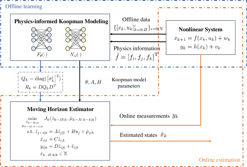
Figure 2: Overview of the proposed learning-based self-tuning Koopman MHE.

In this section, we develop a learning-based self-tuning moving horizon estimation (MHE) method based on the established Koopman model to efficiently estimate the full state of the nonlinear system in (8) in real-time. In this method, we propose a self-tuning weighting matrix update strategy that updates the weighting matrices of the MHE-based estimator for improved estimation performance. The proposed learning-based self-tuning MHE and its connection to the offline physics-informed Koopman modeling is illustrated in Figure 2. In this figure, the blue solid lines indicate parameters updated at each sampling instant, while the black lines represent parameters that remain constant throughout the state estimation process.

At each sampling instant $k\geq H$, the self-tuning MHE estimator aims to find a sequence of optimal estimates $\hat{x}_{k-H|k},\dots,\hat{x}_{k|k}$ based on the output measurements within a time window of size $H$, that is, vector $y_{k-H:k}$. The optimization problem associated with the self-tuning MHE is as follows:

$$\min_{\underset{\hat{z}_{k-H|k},\ \hat{\mu}_{k-H:k-1|k}}{}} J_{k}(\hat{z}_{k-H|k},\hat{\mu}_{k-H:k-1|k})$$ (23a)

$$\text{s.t.}\ \hat{z}_{j+1|k} =A\hat{z}_{j|k}+Bu_{j}+\hat{\mu}_{j|k},\ j=k-H,\dots,k-1$$ (23b)

$$\hat{x}_{i|k} =C\hat{z}_{i|k}$$ (23c)

$$y_{i|k} =D\hat{z}_{i|k}+\hat{v}_{i|k},\ i=k-H,\dots,k$$ (23d)

$$\hat{x}_{k-H:k|k} \in\mathbb{X}$$ (23e)

where the objective function $J_{k}$ is adapted from [39] as follows:

$$J_{k}(\hat{z}_{k-H|k},\hat{\mu}_{k-H:k-1|k})=||\hat{z}_{k-H|k}-\bar{z}_{k-H}||^{2}+\sum_{j=k-H}^{k-1}l(\hat{\mu}_{j|k},\hat{v}_{j|k})+\max_{\underset{j\in k-N:k-1}{}}l(\hat{\mu}_{j|k},\hat{v}_{j|k})$$ (24)

with stage costs

$$l(\hat{\mu}_{j|k},\hat{v}_{j|k})=||\hat{\mu}_{j|k}||_{Q_{k}^{-1}}^{2}+||\hat{v}_{j|k}||_{R_{k}^{-1}}^{2}$$ (25)

In (23)-(25), $\hat{z}_{k-H:k|k}$ and $\hat{\mu}_{k-H:k-1|k}$ are the sequences of the estimates of the lifted state and the estimate of the disturbances in the lifted state-space, respectively. $\hat{z}_{k-H|k}$ and $\hat{\mu}_{k-H:k-1|k}$ are obtained by solving the optimal problem (23), $\hat{v}_{j|k}$ is an estimate of the mismatch of the output measurement equation in the lifted space for time instant $j$ obtained at time $k$. The first term on the right-hand side of (24) is the arrival cost that summarizes the historical information prior to the current estimation window [40], where $\bar{z}_{k-H}$ is the a priori estimate of $z_{k-H}$ computed following $\bar{z}_{k-H}=A\hat{z}_{k-H-1|k-1}+Bu_{k-H-1}$.

The third term on the right-hand side of the objective function in (24) plays an important role in improving the robustness of the estimates [15, 39]. $Q_{k}$ and $R_{k}$ are weighting matrices which are updated at each sampling instant $k$. These two matrices are created based on the output of the pre-trained noise characterization network $N_{\alpha}(\cdot)$. As described in Figure 2, at each sampling instant $k$, $N_{\alpha}(\bar{z}_{k-H})$ outputs $\sigma_{k}^{i}$, $i=1,\dots,n+l$, which are an estimate of the time-varying standard deviation of the disturbances $\mu_{k}$ within the lifted space. $\sigma_{k}^{i}$, $i=1,\dots,n+l$, are used to update weight matrices $Q_{k}$ via (26).

$$Q_{k}=\text{diag}(\left[\sigma_{k}^{i}\right]^{2})$$ (26)

In terms of $R_{k}$, we can use matrix $D$ to convert $Q_{k}$ from the lifted space to the original space. Since we define weight matrices by the noise’s variance, $R_{k}$ is determined by (27).

$$R_{k}=DQ_{k}D^{\text{T}}$$ (27)

Remark 2

To update $Q$ and $R$, the input to $N_{\alpha}(\cdot)$ is the initial prediction $\bar{z}_{k-H}$ that is generated at the previous stage $k-1$ since the only available full state information is the estimation obtained in the previous step.

We note that the weighting matrix for the arrival cost is set to an identity matrix. Additionally, before conducting the estimation, we scale the data to have a mean of 0 and a standard deviation of 1. Therefore, the weight matrices should be close to $\bf{I}$, and weights across different dimensions should not differ by many orders of magnitude, because the estimation is implemented in the scaled space. In application, after taking the inverse of $Q_{k}$, we apply normalization to scale all the elements of $Q_{k}$ to a relatively small range centered around $1$. Then, we use the scaled $Q_{k}$ to compute $R_{k}$. This ensures that the elements of the weighting matrices for both the arrival costs and the stage costs are of similar magnitudes.

5 Application to a chemical process

In this section, a benchmark chemical process is utilized to illustrate the efficacy and superiority of the proposed physics-informed Koopman modeling and learning-based moving horizon estimation method.

5.1 Process description

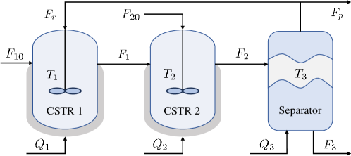
Figure 3: Reactor-separator chemical process.

This benchmark chemical process involves two continuously stirred tank reactors (CSTRs) and one flash tank separator. A schematic view of this process is shown in Figure 3. In this process, reactant A is converted into desired product B, while a portion of B is further transformed into side product C. The two chemical reactions characterized as $\text{A}\to\text{B}$ and $\text{B}\to\text{C}$ take place simultaneously within the two CSTRs. A fresh feed flow containing reactant A is introduced into CSTR 1 at flow rate $F_{10}$ and temperature $T_{10}$. The effluent of CSTR 1 flows into CSTR 2 at flow rate $F_{1}$ and temperature $T_{1}$, while another feed stream carrying pure A enters CSTR 2 at flow rate $F_{20}$ and temperature $T_{20}$. The effluent of CSTR 2 is directed to the separator at flow rate $F_{2}$ and temperature $T_{2}$. The separator has a recycle stream back to the first vessel at flow rate $F_{r}$ and temperature $T_{3}$. Each of the three vessels has a heating jacket, which can add heat to/remove heat from the corresponding vessel at heating input rate, $Q_{i},~{}i=1,2,3$, respectively. The state vector $x$ of this process encompasses nine state variables, specifically, $x=[x_{\text{A}1},x_{\text{B}1},T_{1},x_{\text{A}2},x_{\text{B}2},T_{2},x_{\text{A}3},x_{\text{B}3},T_{3}]^{\text{T}}$, where $x_{\text{A}i}$ and $x_{\text{B}i}$, denote the mass fractions of A and B in the the $i$th vessel, $T_{i}$ represents the temperature in the $i$th vessel, $i=1,2,3$. Nine ordinary differential equations (ODEs) are established to describe the process dynamic behaviors based on material and energy balances, as follows [41]:

$$\displaystyle{\frac{dx_{\text{A}1}}{dt}}=\frac{F_{10}}{V_{1}}(x_{\text{A}10}-x_{\text{A}1})+\frac{F_{r}}{V_{1}}(x_{\text{A}r}-x_{\text{A}1})-k_{1}e^{\frac{-E_{1}}{RT_{1}}}x_{\text{A}1}$$ (28a)

$$\displaystyle{\frac{dx_{\text{B}1}}{dt}}=\frac{F_{10}}{V_{1}}(x_{\text{B}10}-x_{\text{B}1})+\frac{F_{r}}{V_{1}}(x_{\text{B}r}-x_{\text{B}1})+k_{1}e^{\frac{-E_{1}}{RT_{1}}}x_{\text{A}1}-k_{2}e^{\frac{-E_{2}}{RT_{1}}}x_{\text{B}1}$$ (28b)

$$\displaystyle{~{}~{}\frac{dT_{1}}{dt}}=\frac{F_{10}}{V_{1}}(T_{10}-T_{1})+\frac{F_{r}}{V_{1}}(T_{3}-T_{1})-\frac{\Delta H_{1}}{c_{p}}k_{1}e^{\frac{-E_{1}}{RT_{1}}}x_{\text{A}1}-\frac{\Delta H_{2}}{c_{p}}k_{2}e^{\frac{-E_{2}}{RT_{1}}}x_{\text{B}1}+\frac{Q_{1}}{\rho c_{p}V_{1}}$$ (28c)

$$\displaystyle{\frac{dx_{\text{A}2}}{dt}}=\frac{F_{1}}{V_{2}}(x_{\text{A}1}-x_{\text{A}2})+\frac{F_{20}}{V_{2}}(x_{\text{A}20}-x_{\text{A}2})-k_{1}e^{\frac{-E_{1}}{RT_{2}}}x_{\text{A}2}$$ (28d)

$$\displaystyle{\frac{dx_{\text{B}2}}{dt}}=\frac{F_{1}}{V_{2}}(x_{\text{B}1}-x_{\text{B}2})+\frac{F_{20}}{V_{2}}(x_{\text{B}20}-x_{\text{B}2})+k_{1}e^{\frac{-E_{1}}{RT_{2}}}x_{\text{A}2}-k_{2}e^{\frac{-E_{2}}{RT_{2}}}x_{\text{B}2}$$ (28e)

$$\displaystyle{~{}~{}\frac{dT_{2}}{dt}}=\frac{F_{1}}{V_{2}}(T_{1}-T_{2})+\frac{F_{20}}{V_{2}}(T_{20}-T_{2})-\frac{\Delta H_{1}}{c_{p}}k_{1}e^{\frac{-E_{1}}{RT_{2}}}x_{\text{A}2}-\frac{\Delta H_{2}}{c_{p}}k_{2}e^{\frac{-E_{2}}{RT_{2}}}x_{\text{B}2}+\frac{Q_{2}}{\rho c_{p}V_{2}}$$ (28f)

$$\displaystyle{\frac{dx_{\text{A}3}}{dt}}=\frac{F_{2}}{V_{3}}(x_{\text{A}2}-x_{\text{A}3})-\frac{(F_{r}+F_{p})}{V_{3}}(x_{\text{A}r}-x_{\text{A}3})$$ (28g)

$$\displaystyle{\frac{dx_{\text{B}3}}{dt}}=\frac{F_{2}}{V_{3}}(x_{\text{B}2}-x_{\text{B}3})-\frac{(F_{r}+F_{p})}{V_{3}}(x_{\text{B}r}-x_{\text{B}3})$$ (28h)

$$\displaystyle{~{}~{}\frac{dT_{3}}{dt}}=\frac{F_{2}}{V_{3}}(T_{2}-T_{3})+\frac{Q_{3}}{\rho c_{p}V_{3}}+\frac{(F_{r}+F_{p})}{\rho c_{p}V_{3}}(x_{\text{A}r}\Delta H_{\text{vap1}}+x_{\text{B}r}\Delta H_{\text{vap2}}+x_{\text{C}r}\Delta H_{\text{vap3}})$$ (28i)

where $x_{\text{A}10}$, $x_{\text{B}10}$ are the mass fractions of A and B in the feed flow; $x_{\text{A}r}$, $x_{\text{B}r}$, $x_{\text{C}r}$ are the mass fractions of A, B, C in the recycle flow; $F_{1}$ and $F_{2}$ represent the effluent flow rates from vessels 1 and 2; $F_{r}$, $F_{p}$ are the flow rates of the recycle flow and purge flow, respectively; $V_{1}$, $V_{2}$, $V_{3}$ are the volumes of the three vessels; $E_{1}$, $E_{2}$ are the activation energy for the two reactions; $k_{1}$, $k_{2}$ are the pre-exponential values for reactions 1, 2; $\Delta H_{1}$, $\Delta H_{2}$ are heats of reaction for the two reactions; $c_{p}$ represents the heat capacity; $r$ is the gas constant; $\rho$ is the solution density.

Furthermore, we use $x_{\text{C}3}$ to represent the mass fraction of C in the separator, and the algebraic equation describing the relationship between the composition of the overhead stream and the liquid composition in the separator are given as follows:

$$x_{\text{A}r} =\frac{\alpha_{\text{A}}x_{\text{A}3}}{\alpha_{\text{A}}x_{\text{A}3}+\alpha_{\text{B}}x_{\text{B}3}+\alpha_{\text{C}}x_{\text{C}3}}$$ (29a)

$$x_{\text{B}r} =\frac{\alpha_{\text{B}}x_{\text{B}3}}{\alpha_{\text{A}}x_{\text{A}3}+\alpha_{\text{B}}x_{\text{B}3}+\alpha_{\text{C}}x_{\text{C}3}}$$ (29b)

$$x_{\text{C}r} =\frac{\alpha_{\text{C}}x_{\text{C}3}}{\alpha_{\text{A}}x_{\text{A}3}+\alpha_{\text{B}}x_{\text{B}3}+\alpha_{\text{C}}x_{\text{C}3}}$$ (29c)

More detailed process descriptions and the adopted process parameters can be found in [41]. The dynamic model in (28) is used as a simulator for data generation. Additionally, in this work, we consider practical scenarios when only partial equations of (28) are available, which will be detailed in the subsequent subsection. The available physical information and the simulated data are jointly used for building a Koopman model that describes the dynamics of the process in a linear manner.

5.2 Simulation settings

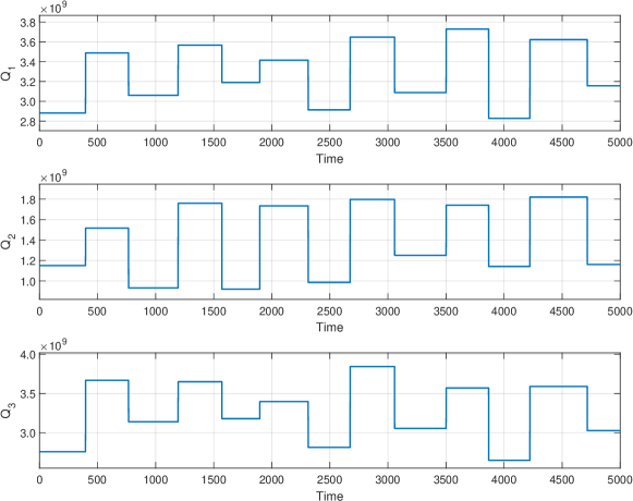
Figure 4: Pattern of Heat Inputs for Dataset Generation.

To illustrate the proposed modeling approach, we consider that among (28), only the ODEs that describe the dynamic behaviors of the temperatures in the three vessels are known, that is (28c), (28f), and (28i) are available, while the remaining ODEs are unavailable. Consequently, $\tilde{f}=[f_{3},f_{6},f_{9}]^{\text{T}}$, where $f_{3}$, $f_{6}$, $f_{9}$ are the right-hand sides of (28c), (28f), and (28i), respectively. The available physical information $\tilde{f}$ will be leveraged for learning-based physics-informed Koopman modeling.

We consider a steady-state point $x_{s}=[0.1763,0.6731,$ $480.3165~{}\text{K},$ $0.1965,0.6536,472.7863~{}\text{K},$ $0.0651,0.6703,474.8877~{}\text{K}]^{\text{T}}$. The initial state $x_{0}$ is uniformly sampled from the range of $[x_{s},1.2x_{s}]$. Considering the different magnitudes of the nine state variables of this process, disturbances of different magnitudes are added to states with respect to the mass fractions and temperatures. The system disturbances $w$ to the original system (8) are generated following Gaussian distributions, and are then made bounded. Specifically, the sequence of disturbance added to each state related to mass fractions is generated following $\mathcal{N}(0,0.5)$, and then made bounded within $[-5,5]$ in each dimension, while the disturbance added to each state related to temperature is generated following $\mathcal{N}(0,10)$ and is then made bounded within $[-10,10]$.

The state measurements are sampled at intervals $\Delta=0.001$ hours. We use (28) to generate a dataset for the Koopman model training through open-loop simulations. The heat inputs $Q_{i},i=1,2,3$ are set to random values with added Gaussian noise $\mathcal{N}(0,10^{2}\times\bf{I}_{3})$ which is bounded by $[-10^{3},10^{3}]\times\bf{I}_{3}$. To ensure comprehensive coverage of system states in the simulated dataset, the duration of each input’s mean state is randomly selected between 0.2 to 0.5 hours, as depicted in Figure 4. The initial values of the heat inputs and the randomly chosen input values disregarding noise at each time step are selected within the upper bounds $u_{max}$ and lower bounds $u_{min}$, as indicated in Table 1.

Table 1: The upper bounds and lower bounds of inputs.

Bounds of inputs	$Q_{1}~{}(\text{kJ/h})$	$Q_{2}~{}(\text{kJ/h})$	$Q_{3}~{}(\text{kJ/h})$
$u_{\text{max}}$	$3.2\times 10^{9}$	$1.9\times 10^{9}$	$3.2\times 10^{9}$
$u_{\text{min}}$	$2.8\times 10^{9}$	$0.9\times 10^{9}$	$2.8\times 10^{9}$

While offline data for all the nine process states can be collected for offline modeling, from an online implementation perspective, only the temperatures in the three vessels are measured, that is, $y=[T_{1},T_{2},T_{3}]^{\text{T}}$. Therefore, our objective is to utilize the proposed physics-informed Koopman modeling approach to construct a linear Koopman model to forecast the dynamic behavior of nonlinear system (28). Subsequently, we design a constrained state estimation scheme based on the Koopman model to estimate all the nine system states based on the output measurements in real-time.

5.3 Modeling results

We train the Koopman model using a dataset $\mathcal{D}:=\{[x_{k},u_{k}]_{k=0:20}^{i}\}_{i=0:2000}$. The dataset is then divided into two parts: $80\%$ for training and $20\%$ for validation. Additionally, we generate additional data as a test dataset. A list of the hyperparameters used in model training is provided in Table 2. The trained Koopman model is used for 20-step-ahead open-loop prediction, i.e., $H=20$. The prediction results for the nine states of the process are shown in Figure 5. We set $lr_{1}=0.001$ refers to the learning rate for neural networks $F_{\theta}(\cdot)$ and $N_{\alpha}(\cdot)$, $lr_{2}=0.0001$ which represents the learning rate for matrices $A,B$, $lr_{3}=0.001$ which is the learning rate of weights related parameters of loss function $\nu_{i},i=1,2,3,4$. Different learning rates are chosen for the trainable parameters of the pipeline to improve the performance of the resulting model. The values of these learning rates are determined through mild tuning.

Table 2: Hyperparameters adopted for physics-informed Koopman modeling.

Parameters	Values
The total size of dataset: $\mathcal{D}$	$2000\times 20$
Lifted dimension: $l$	13
Activation function	ReLU
Optimizer	Adam
Learning rate for $F_{\theta}(\cdot)$ and $F_{\theta}(\cdot)$: $lr_{1}$	0.001
Learning rate for matrices $A,B$: $lr_{2}$	0.0001
Learning rate for weights $\nu_{i}$: $lr_{3}$	0.001

Additionally, we compare the proposed physics-informed modeling method with the purely data-driven learning-based Koopman modeling method [42, 31]. The major difference between our method and the baseline is that our method incorporates physics-informed loss terms into the final loss function, whereas the baseline is optimized solely using the collected dataset. Both models are trained on the same dataset $\mathcal{D}$. The comparative modeling result of open-loop Koopman model prediction is shown in Figure 5. The proposed method provides smaller prediction errors as compared to the baseline.

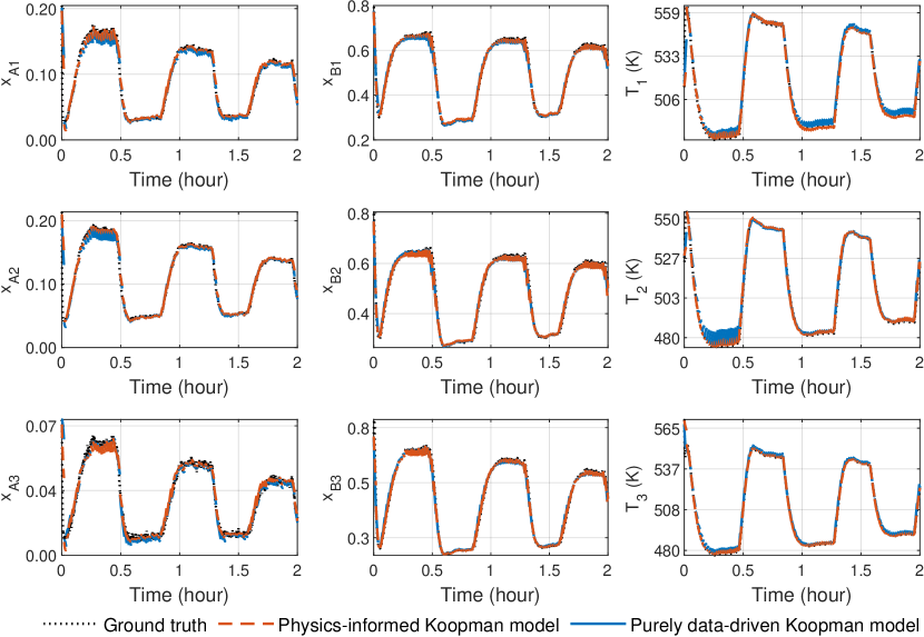
Figure 5: The comparison modeling result of open-loop Koopmen model prediction.

We randomly generated several different datasets with different initial values of states $x_{0}$ and input $u_{0}$. Using each dataset, we repeat the training process 10 times, and average the loss values. The results are presented in Figure 6.

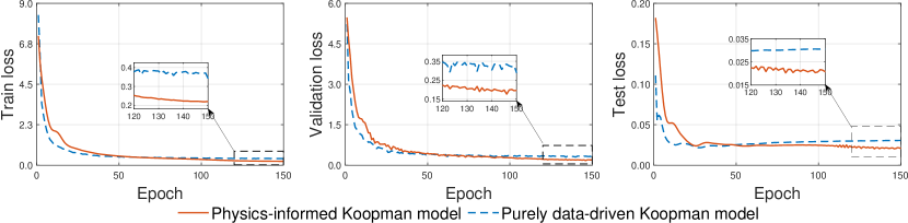
Figure 6: Mean loss curve of train, validation, and test for Koopman model training.

Through repeated simulations, the training results demonstrate consistent results: 1) The physics-informed Koopman modeling method effectively mitigates overfitting. As depicted in Figure 6, the test loss of physics-informed Koopman decreases with epoch, and the test loss curve of the pure data-driven Koopman increases obviously. This may be because the scale of the dataset is not large, and the trained model may exhibit different behaviors in validation and test scenarios for the purely data-driven method. 2) The physics-informed Koopman model achieves smaller minimum values in the training loss, the validation loss, and the test loss. We use mean squared error (MSE) as the criterion, the average test loss for the proposed method is 30% smaller than the purely data-driven baseline.

Remark 3

The difference in the order of magnitude between the test loss and the other two kinds of losses arises from the use of different assessment metrics. The train and validation losses are calculated based on the weighted sum of $\mathcal{L}_{x}$ and $\mathcal{L}_{z}$, while the test loss is the mean square error between the true and predicted test states, which is the same as $\mathcal{L}_{x}$. Also, to facilitate the convergence of the trained model, we set an initial weight to each loss term to normalize the order of magnitudes. In this process, we set the weights of $\mathcal{L}_{x}$ and $\mathcal{L}_{z}$ as 10.

5.4 State estimation results

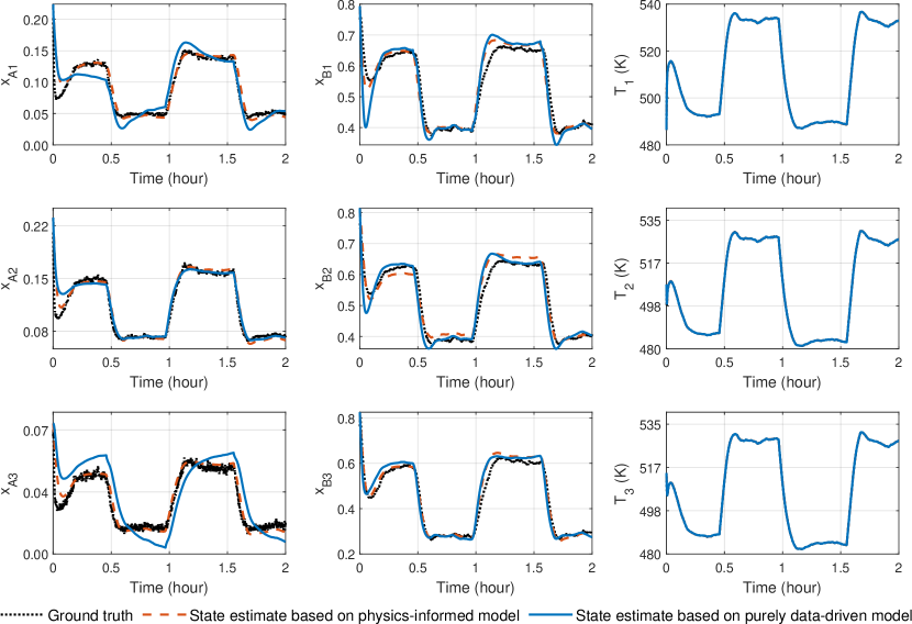
Figure 7: State estimation results generated with Koopman and physics-informed Koopman models.

Based on the Koopman model, an MHE scheme with self-tuning weighting matrices is developed. We generate additional datasets through simulating (28) for testing the performance of the MHE scheme. In the online implementation, we consider that only the temperatures are online measured, and we estimate all the nine system states. The output measurement equation $h$ in (8b) is linear, and the matrix $D$ takes the form $D=\bar{C}C$ where $\bar{C}_{3\times 9}$ has one element of $1$ in each row, corresponding to the temperature measurement in a single vessel, with all other elements being 0. The initial guess used by the estimator is $\hat{z}_{0|0}=1.2z_{0}$. The estimation horizon is 40. The estimation results provided by the proposed method are presented in Figure 7. The state estimates (dashed lines) accurately capture the actual states (dotted lines).

Additionally, we compare the estimation performance of the proposed method with two other Koopman-based MHE designs. Specifically, we consider three methods:1) the proposed self-tuning MHE based on a physics-informed Koopman model, denoted by MHE design 1; 2) MHE based on the physics-informed Koopman model but with constant weighting matrices, denoted by MHE design 2; 3) an MHE design based on purely data-driven Koopman model and with constant weighting matrices, denoted by MHE design 3.

Table 3: The mean squared error (MSE) for each of the three MHE designs.

Method	MSE of the state estimates
MHE design 1 (proposed method)	0.0412
MHE design 2	0.0421
MHE design 3	0.0972

The state estimation results given by MHE design 3 are also shown in Figure 7. While both the proposed method and MHE design 3 can provide estimates that can overall capture the trend of the ground truth, the estimates given by MHE design 1 (the proposed method) are more accurate than MHE design 3. Additional repeated simulations are conducted with different initial states and different input and noise profiles to assess the performance of the three methods. The averaged mean squared errors for the three methods are presented in Table 3. The proposed method achieves the lowest MSE among the three designs, with the MSE of MHE design 1 reduced by 55% compared to MHE design 3 and by 2.1% compared to MHE design 2. The results indicate that with the more accurate physics-informed Koopman model, state estimation accuracy can be substantially reduced. By further updating the weighting matrices of the Koopman MHE online using the proposed method, the estimation accuracy can be further enhanced.

6 Conclusion

In this work, we propose a physics-informed machine learning Koopman modeling approach that leverages both data and available physical information to train the neural network-based lifting functions and Koopman operators. Based on this Koopman model, we formulated a linear self-tuning MHE design to address constrained state estimation of general nonlinear systems. The weighting matrices are updated using a pre-trained neural network, which is constructed during the offline Koopman modeling phase. Only convex optimization is required for implementing the MHE-based constrained estimation scheme online, despite the nonlinear dynamics of the considered system. On a benchmark chemical process, the proposed Koopman modeling and estimation approach is able to show superior performance. The physics-informed modeling method provides enhanced predictive capability and can mitigate overfitting compared to the traditional learning-based Koopman model, especially when dealing with small and noisy datasets. The proposed Koopman-based self-tuning MHE scheme also demonstrates good estimation results. The implementation of the physics-informed Koopman model for MHE and self-tuning of the MHE weighting matrices led to better estimation performance compared to the two baseline Koopman-based MHE methods considered.

References

- [1] Bernard O Koopman. Hamiltonian systems and transformation in Hilbert space. Proceedings of the National Academy of Sciences, 17(5):315–318, 1931.
- [2] Xuewen Zhang, Minghao Han, and Xunyuan Yin. Reduced-order Koopman modeling and predictive control of nonlinear processes. Computers & Chemical Engineering, 179:108440, 2023.
- [3] Milan Korda and Igor Mezić. Linear predictors for nonlinear dynamical systems: Koopman operator meets model predictive control. Automatica, 93:149–160, 2018.
- [4] Carl Folkestad and Joel W Burdick. Koopman nmpc: Koopman-based learning and nonlinear model predictive control of control-affine systems. In IEEE International Conference on Robotics and Automation (ICRA), pages 7350–7356, 2021.
- [5] Hassan Arbabi, Milan Korda, and Igor Mezić. A data-driven Koopman model predictive control framework for nonlinear partial differential equations. In 2018 IEEE Conference on Decision and Control (CDC), pages 6409–6414. IEEE, 2018.
- [6] Xinglong Zhang, Wei Pan, Riccardo Scattolini, Shuyou Yu, and Xin Xu. Robust tube-based model predictive control with Koopman operators. Automatica, 137:110114, 2022.
- [7] Minghao Han, Zhaojian Li, Xiang Yin, and Xunyuan Yin. Robust learning and control of time-delay nonlinear systems with deep recurrent Koopman operators. IEEE Transactions on Industrial Informatics, 20(3):4675–4684, 2024.
- [8] Minghao Han, Jingshi Yao, Adrian Wing-Keung Law, and Xunyuan Yin. Efficient economic model predictive control of water treatment process with learning-based Koopman operator. Control Engineering Practice, 149:105975, 2024.
- [9] Xunyuan Yin and Jinfeng Liu. Subsystem decomposition of process networks for simultaneous distributed state estimation and control. AIChE Journal, 65(3):904–914, 2019.
- [10] Xiaojie Li, Adrian Wing-Keung Law, and Xunyuan Yin. Partition-based distributed extended Kalman filter for large-scale nonlinear processes with application to chemical and wastewater treatment processes. AIChE Journal, 69(12):e18229, 2023.
- [11] Xunyuan Yin and Jinfeng Liu. State estimation of wastewater treatment plants based on model approximation. Computers & Chemical Engineering, 111:79–91, 2018.
- [12] Zhaoyang Duan and Costas Kravaris. Nonlinear observer design for two-time-scale systems. AIChE Journal, 66(6):e16956, 2020.
- [13] Xunyuan Yin, Jing Zeng, and Jinfeng Liu. Forming distributed state estimation network from decentralized estimators. IEEE Transactions on Control Systems Technology, 27(6):2430–2443, 2019.
- [14] Wentao Tang. Data-driven state observation for nonlinear systems based on online learning. AIChE Journal, 69(12):e18224, 2023.
- [15] Christopher V Rao, James B Rawlings, and David Q Mayne. Constrained state estimation for nonlinear discrete-time systems: Stability and moving horizon approximations. IEEE Transactions on Automatic Control, 48(2):246–258, 2003.
- [16] Wentao Tang and Prodromos Daoutidis. Nonlinear state and parameter estimation using derivative information: A Lie-Sobolev approach. Computers & Chemical Engineering, 151:107369, 2021.
- [17] Mohammed S Alhajeri, Zhe Wu, David Rincon, Fahad Albalawi, and Panagiotis D Christofides. Machine-learning-based state estimation and predictive control of nonlinear processes. Chemical Engineering Research and Design, 167:268–280, 2021.
- [18] Matthew O Williams, Ioannis G Kevrekidis, and Clarence W Rowley. A data-driven approximation of the Koopman operator: Extending dynamic mode decomposition. Journal of Nonlinear Science, 25:1307–1346, 2015.
- [19] Sang Hwan Son, Hyun-Kyu Choi, Jiyoung Moon, and Joseph Sang-Il Kwon. Hybrid Koopman model predictive control of nonlinear systems using multiple edmd models: An application to a batch pulp digester with feed fluctuation. Control Engineering Practice, 118:104956, 2022.
- [20] Yoshinobu Kawahara. Dynamic mode decomposition with reproducing kernels for Koopman spectral analysis. Advances in Neural Information Processing Systems, 29, 2016.
- [21] Xunyuan Yin, Yan Qin, Jinfeng Liu, and Biao Huang. Data-driven moving horizon state estimation of nonlinear processes using Koopman operator. Chemical Engineering Research and Design, 200:481–492, 2023.
- [22] Haojie Shi and Max Q-H Meng. Deep Koopman operator with control for nonlinear systems. IEEE Robotics and Automation Letters, 7(3):7700–7707, 2022.
- [23] Kadir Liano. Robust error measure for supervised neural network learning with outliers. IEEE Transactions on Neural Networks, 7(1):246–250, 1996.
- [24] George Em Karniadakis, Ioannis G Kevrekidis, Lu Lu, Paris Perdikaris, Sifan Wang, and Liu Yang. Physics-informed machine learning. Nature Reviews Physics, 3(6):422–440, 2021.
- [25] Eric Aislan Antonelo, Eduardo Camponogara, Laio Oriel Seman, Jean Panaioti Jordanou, Eduardo Rehbein de Souza, and Jomi Fred Hübner. Physics-informed neural nets for control of dynamical systems. Neurocomputing, page 127419, 2024.
- [26] Jonas Nicodemus, Jonas Kneifl, Jörg Fehr, and Benjamin Unger. Physics-informed neural networks-based model predictive control for multi-link manipulators. IFAC-PapersOnLine, 55(20):331–336, 2022.
- [27] Ming Xiao and Zhe Wu. Modeling and control of a chemical process network using physics-informed transfer learning. Industrial & Engineering Chemistry Research, 62(42):17216–17227, 2023.
- [28] Xue Ying. An overview of overfitting and its solutions. In Journal of Physics: Conference Series, volume 1168, page 022022. IOP Publishing, 2019.
- [29] Minghao Han, Jacob Euler-Rolle, and Robert K Katzschmann. DeSKO: Stability-assured robust control with a deep stochastic Koopman operator. In International Conference on Learning Representations, 2021.
- [30] Enoch Yeung, Soumya Kundu, and Nathan Hodas. Learning deep neural network representations for Koopman operators of nonlinear dynamical systems. In American Control Conference (ACC), pages 4832–4839. IEEE, 2019.
- [31] Yiqiang Han, Wenjian Hao, and Umesh Vaidya. Deep learning of Koopman representation for control. In IEEE Conference on Decision and Control, pages 1890–1895, 2020.
- [32] Yongqian Xiao, Xinglong Zhang, Xin Xu, Xueqing Liu, and Jiahang Liu. Deep neural networks with Koopman operators for modeling and control of autonomous vehicles. IEEE Transactions on Intelligent Vehicles, 8(1):135–146, 2022.
- [33] Jonathan H Tu. Dynamic mode decomposition: Theory and applications. PhD thesis, Princeton University, 2013.
- [34] Peter L Bartlett and Wolfgang Maass. Vapnik-chervonenkis dimension of neural nets. The Handbook of Brain Theory and Neural Networks, pages 1188–1192, 2003.
- [35] Junghwan Cho, Kyewook Lee, Ellie Shin, Garry Choy, and Synho Do. How much data is needed to train a medical image deep learning system to achieve necessary high accuracy? arXiv preprint arXiv:1511.06348, 2015.
- [36] Alex Kendall and Yarin Gal. What uncertainties do we need in Bayesian deep learning for computer vision? Advances in neural information processing systems, 30, 2017.
- [37] Alex Kendall, Yarin Gal, and Roberto Cipolla. Multi-task learning using uncertainty to weigh losses for scene geometry and semantics. In Proceedings of the IEEE Conference on Computer Vision and Pattern Recognition, pages 7482–7491, 2018.
- [38] Lukas Liebel and Marco Körner. Auxiliary tasks in multi-task learning. arXiv preprint arXiv:1805.06334, 2018.
- [39] Matthias A Müller. Nonlinear moving horizon estimation in the presence of bounded disturbances. Automatica, 79:306–314, 2017.
- [40] Angelo Alessandri, Marco Baglietto, and Giorgio Battistelli. Robust receding-horizon state estimation for uncertain discrete-time linear systems. Systems & Control Letters, 54(7):627–643, 2005.
- [41] Jing Zhang and Jinfeng Liu. Distributed moving horizon state estimation for nonlinear systems with bounded uncertainties. Journal of Process Control, 23(9):1281–1295, 2013.
- [42] Bethany Lusch, J Nathan Kutz, and Steven L Brunton. Deep learning for universal linear embeddings of nonlinear dynamics. Nature Communications, 9(1):4950, 2018.