Probing radiative electroweak symmetry breaking with colliders and gravitational waves

Abstract

Radiative symmetry breaking provides an appealing explanation for electroweak symmetry breaking and addresses the hierarchy problem. We present a comprehensive phenomenological study of this scenario, focusing on its key feature: the logarithmic-shaped potential. This potential gives rise to a relatively light scalar boson that mixes with the Higgs boson and leads to first-order phase transitions (FOPTs) in the early Universe. Our detailed analysis includes providing exact and analytical solutions for the vacuum structure and scalar interactions, classifying four patterns of cosmic thermal history, and calculating the supercooled FOPT dynamics and GWs. By combining future collider and gravitational wave experiments, we can probe the conformal symmetry breaking scales up to $10^{5}-10^{8}$ GeV.

I Introduction

The discovery of the Higgs boson at the Large Hadron Collider (LHC) Aad et al. (2012); Chatrchyan et al. (2012) represents a significant milestone in understanding fundamental particles and their interactions. However, the mechanism of electroweak symmetry breaking (EWSB) remains a mystery. In the Standard Model (SM), EWSB is achieved through a negative mass squared term in the Higgs potential. While minimal and economical, it lacks a fundamental explanation for this term’s origin. This bare mass term is sensitive to ultraviolet (UV) physics, necessitating finely-tuned UV parameters to yield a Higgs mass of 125 GeV. This is the well-known hierarchy problem that has motivated the exploration of physics beyond the SM (BSM), including theories such as supersymmetry, composite Higgs, and extra dimensions.

Radiative symmetry breaking offers a viable explanation for EWSB and addressing the hierarchy problem Coleman and Weinberg (1973); Jackiw (1974); Bardeen (1995); Meissner and Nicolai (2008); de Boer et al. (2024); Frasca et al. (2024). In this framework, the Lagrangian does not contain dimensionful parameters at tree-level, and hence is classically scale-invariant or conformal. At the one-loop level, radiative corrections induce a logarithmic contribution to the scalar potential, leading to spontaneous symmetry breaking. This effect arises from quantum corrections, characterizing it as an anomaly. It can also be interpreted as dimensional transmutation resulting from the renormalization group running of the scalar couplings.

While the concept of radiative symmetry breaking is appealing, its direct application to the SM without extending the particle content results in a Higgs boson mass of $\lesssim 10$ GeV (excluding the top quark contribution) or an unstable electroweak (EW) vacuum (including the top quark contribution), both of which conflict with experimental data. To align with Higgs measurements, the framework has been modified so that radiative symmetry breaking occurs in a BSM sector and is transmitted to the SM via Higgs-portal couplings, thereby inducing EWSB Hempfling (1996). This mechanism also presents potential solutions to longstanding problems in particle physics, including neutrino mass Iso et al. (2009a, b); Chun et al. (2013); Das et al. (2017), matter-antimatter asymmetry Khoze and Ro (2013); Davoudiasl and Lewis (2014); Huang and Xie (2022); Chun et al. (2023), and dark matter Okada and Orikasa (2012); Hambye and Strumia (2013); Hambye et al. (2018); Baldes and Garcia-Cely (2019); Yaser Ayazi and Mohamadnejad (2019); Mohamadnejad (2020); Khoze and Milne (2023); Frandsen et al. (2023); Wong and Xie (2023) or primordial black holes Gouttenoire (2024); Salvio (2024, 2023); Conaci et al. (2024); Banerjee et al. (2024).

In this study, we examine the phenomenology of radiative EWSB. The distinctive feature of this scenario is the logarithmic potential of the BSM scalar field $\phi$, leading to two types of specific phenomenological signals. First, field excitation near the vacuum produces a scalar boson with mass significantly lighter than the BSM scale $w$, which can be detected at current or future particle colliders. Second, the flat potential near the origin results in one or more first-order phase transitions (FOPTs) in the early Universe, creating stochastic gravitational waves (GWs) observable today. By analyzing these signals, we aim to identify the signatures of the radiative symmetry breaking mechanism.

Our research shows several novelties. First, we provide a fully analytical solution for the vacuum structure, scalar mixings, and interactions, assuming sequential symmetry breaking when $w\gg$ the EW scale. Second, unlike previous studies that typically impose specific assumptions on vector couplings to the SM particles (e.g. embedding models in gauged $U(1)_{B-L}$ or kinetic mixing frameworks), we concentrate on the fundamental concept of radiative EWSB, i.e. the interaction between the SM Higgs boson and the new scalar, as well as the logarithmic shape of the scalar potential. Third, we combine collider and GW searches. The projected reach of HL-LHC and future 10 TeV muon collider is evaluated. In parallel, we conduct a detailed analysis of the FOPT dynamics, classifying different patterns of the cosmic thermal history, and evaluating the associated GWs. Our findings indicate that collider and GW searches are largely complementary across the parameter space, with opportunities for crosscheck in certain regions.

This article is organized as follows. In Section II, we introduce the benchmark model and analyze its vacuum structure, establishing the framework for the phenomenological study. Section III focuses on collider phenomenology, while Section IV investigates the dynamics of FOPT and the generation of GWs. We combine the findings from the collider and GW analyses, presenting the final results in Section V. The conclusion is given in Section VI.

II The model

The tree-level joint potential of the SM Higgs doublet $H=\left(G^{+},(h+iG^{0})/\sqrt{2}\right)^{T}$ and the real scalar field $\phi$ reads

$$V_{0}(H,S)=\lambda_{h}|H|^{4}+\frac{\lambda_{s}}{4}\phi^{4}+\frac{\lambda_{h\phi}}{2}|H|^{2}\phi^{2},$$ (1)

where all the coefficients are dimensionless, and hence the theory is classically conformal. One-loop correction generates logarithmic contributions to Eq. (1), known as the Coleman-Weinberg potentials Coleman and Weinberg (1973); Jackiw (1974); Gildener and Weinberg (1976). In principle, both $H$ and $\phi$ receive radiative corrections, resulting in a complicated joint potential. However, under the assumption that the BSM scale significantly exceeds the EW scale and that the magnitude of Higgs-portal coupling $|\lambda_{h\phi}|\ll 1$, we can establish a sequential symmetry breaking scenario Chataignier et al. (2018): the BSM radiative correction to the $\phi$-direction generates the spontaneous symmetry breaking at a high scale, which then induces a tree-level potential along the $h$-direction via the $\lambda_{h\phi}$-term, producing the EWSB.

In this case, the potential in unitary gauge up to one-loop level can be written as

$$V_{1}(h,\phi)=\frac{B}{4}\phi^{4}\left(\log\frac{\phi}{w_{0}}-\frac{1}{4}\right)+\frac{\lambda_{h\phi}}{4}h^{2}\phi^{2}+\frac{\lambda_{h}}{4}h^{4},$$ (2)

which implies different dominance of tree- and loop-level contributions in different field directions. Along the $\phi$-direction, the loop-induced logarithmic potential dominates and generates the conformal symmetry breaking, resulting in $\left\langle\phi\right\rangle\approx w_{0}$ and a scalar boson with a mass of $m_{\phi}\approx\sqrt{B}w_{0}$. While along the $h$-direction, it is the tree-level contribution that dominates: after $\phi$ acquires its vacuum expectation value (VEV), a Mexican-hat-shaped Higgs potential

$$V_{h}(h)\approx V_{1}(h,w_{0})=\frac{1}{4}(\lambda_{h\phi}w_{0}^{2}h^{2}+\lambda_{h}h^{4})$$ (3)

is generated. Setting the parameters as $\lambda_{h\phi}\approx-m_{h}^{2}/w_{0}^{2}$ and $\lambda_{h}\approx m_{h}^{2}/(2v^{2})$ with $m_{h}=125$ GeV and $v=246$ GeV, we then get the EWSB with correct Higgs mass and VEV.

The parameter $B$ is contributed by the new physics degrees of freedom in the BSM sector. In the minimal model-building sense, there are two alternative scenarios: gauge-induced or scalar-induced. In the former case, $\phi$ is embedded to a complex scalar $S=(\phi+i\eta)/\sqrt{2}$ that is charged under a gauged dark $U(1)_{X}$ with the coupling constant $g_{X}$; while in the latter case, $\phi$ couples to a dark real scalar $X$ via the quartic interaction $\lambda_{X}\phi^{2}X^{2}/4$ in the tree-level potential. Then

$$B=\begin{dcases}\frac{3g_{X}^{4}}{8\pi^{2}},&\text{for the gauge-induced scenario;}\\ \frac{\lambda_{X}^{2}}{32\pi^{2}},&\text{for the scalar-induced scenario.}\end{dcases}$$ (4)

After the symmetry breaking, the $U(1)_{X}$ gauge boson $Z^{\prime}$ or dark scalar $X$ gets a mass of $m_{Z^{\prime}}\approx g_{X}w_{0}$ or $m_{X}\approx\sqrt{\lambda_{X}}w_{0}/\sqrt{2}$, respectively. BSM fermions coupling to $\phi$ make negative and suppressed contributions to $B$. For example, if we embed the model into a gauged $U(1)_{B-L}$ framework in which $g_{X}=2g_{B-L}$ and the right-handed neutrino interactions read $-\sum_{i}y_{i}S\bar{\nu}_{R}^{i,c}\nu_{R}^{i}/2+{\rm h.c.}$ Iso et al. (2009a, b), then $B\propto(g_{B-L}^{4}-\sum_{i}y_{i}^{4}/96)$. Therefore, the bosonic BSM degrees of freedom dominate $B$, and we will consider the two minimal realizations in Eq. (4) as research benchmarks. As will be demonstrated, the particle phenomenology of $\phi$ is independent of the source of $B$, and the GW signals are likewise insensitive to its origin. Therefore, we will not specify the explicit expression for $B$ in our discussion unless necessary.

While the above description shows a very clear qualitative picture of the symmetry breaking pattern, it neglects the impact of the Higgs-portal coupling on the $\phi$-direction potential, which causes the mixing between $\phi$ and $h$. That is why we used “$\approx$” when discussing the VEVs and particle masses around Eq. (3). Below we resolve the vacuum structure using the full expression of Eq. (2), providing the exact and analytical solution for scalar VEVs, masses, and mixing angle. Let $\left\langle h\right\rangle=v$ and $\left\langle\phi\right\rangle=w$ be the vacuum where $\partial V_{1}/\partial h$ and $\partial V_{1}/\partial\phi$ vanish, we find

$$\lambda_{h\phi}=-2B\frac{w^{2}}{v^{2}}\ln\frac{w}{w_{0}},\quad\lambda_{h}=B\frac{w^{4}}{v^{4}}\ln\frac{w}{w_{0}}.$$ (5)

Since $\lambda_{h}>0$ is required from the bounded below condition, one can infer $w>w_{0}$, thus the $\phi$ VEV is larger than the bare parameter $w_{0}$.

Next, we diagonalize the Hessian matrix

$${\rm Hes} = \begin{pmatrix}\frac{\partial^{2}V_{1}}{\partial h^{2}}\,&\frac{\partial^{2}V_{1}}{\partial h\partial\phi}\\[8.5359pt] \frac{\partial^{2}V_{1}}{\partial h\partial\phi}\,&\frac{\partial^{2}V_{1}}{\partial\phi^{2}}\end{pmatrix}_{(v,w)}$$

$$= \begin{pmatrix}3\lambda_{h}v^{2}+\frac{\lambda_{h\phi}}{2}w^{2}&\lambda_{h\phi}vw\\[8.5359pt] \lambda_{h\phi}vw&Bw^{2}+3Bw^{2}\ln\frac{w}{w_{0}}+\frac{\lambda_{h\phi}}{2}v^{2}\end{pmatrix},$$

to get the two scalar mass eigenvalues

$$m_{h_{1,2}}^{2}=\frac{w^{2}}{4}\left(6B\ln\frac{w}{w_{0}}+2B+\lambda_{h\phi}\right)\\ +\frac{v^{2}}{4}(6\lambda_{h}+\lambda_{h\phi})\mp\frac{\Xi^{1/2}}{4},$$ (7)

where

$$\Xi=\left[w^{2}(2B-\lambda_{h\phi})+6Bw^{2}\ln\frac{w}{w_{0}}-v^{2}(6\lambda_{h}-\lambda_{h\phi})\right]^{2}\\ +16\lambda_{h\phi}^{2}v^{2}w^{2}.$$ (8)

Note $m_{h_{2}}>m_{h_{1}}$ by definition, but we do not specify which one is the SM Higgs boson yet.

Substituting Eq. (5) into Eq. (7) to cancel $B$, one obtains

$$\left(1+\frac{w^{2}}{v^{2}}\right)^{2}\xi^{2}+\left(1-\frac{(m_{h_{1}}^{4}+m_{h_{2}}^{4})w^{2}}{2m_{h_{1}}^{2}m_{h_{2}}^{2}v^{2}}\right)\xi+\frac{1}{4}=0,$$ (9)

where $\xi=\ln(w/w_{0})$. Resolving this univariate quadratic equation, one obtains two solutions

$$\ln\frac{w}{w_{0}} = \frac{m_{h_{1}}^{4}v^{2}w^{2}+m_{h_{2}}^{4}v^{2}w^{2}-2m_{h_{1}}^{2}m_{h_{2}}^{2}v^{4}\pm\Delta}{4m_{h_{1}}^{2}m_{h_{2}}^{2}\left(v^{2}+w^{2}\right)^{2}},$$

$$\Delta = v^{2}w^{2}\left(m_{h_{2}}^{4}-m_{h_{1}}^{4}\right)\sqrt{1-\frac{4m_{h_{1}}^{2}m_{h_{2}}^{2}v^{2}}{(m_{h_{2}}^{2}-m_{h_{1}}^{2})^{2}w^{2}}}.\qquad$$ (10)

They correspond to two branches of the physical cases: the “$+$” branch is for a singlet lighter than Higgs while the “$-$” branch is for a singlet heavier than Higgs. Also note that the definition of $\Delta$ requires

$$m_{h_{2}}>m_{h_{1}}\left(\sqrt{1+\frac{v^{2}}{w^{2}}}+\frac{v}{w}\right),$$ (11)

thus the two scalar bosons cannot be degenerate.

One of $h_{1}$ and $h_{2}$ corresponds to the Higgs boson observed at the LHC, while the other represents the new singlet-like boson yet to be discovered. For simplicity, we use the notations $h$ and $\phi$ to denote the Higgs and singlet-like mass eigenstates, respectively, and define the rotation matrix as

$$\begin{pmatrix}h\\ \phi\end{pmatrix}\xrightarrow[\rm eigenstates]{\rm to~{}mass}U\begin{pmatrix}h\\ \phi\end{pmatrix},\quad U=\begin{pmatrix}\cos\theta&\sin\theta\\ -\sin\theta&\cos\theta\end{pmatrix},$$ (12)

where $\theta$ is the mixing angle satisfying $|\theta|<\pi/4$ so that the magnitude of the diagonal elements is larger than that of the non-diagonal ones. The Hessian matrix is diagonalized as $U^{\dagger}{\rm Hes}\,U={\rm diag}\{m_{h}^{2},m_{\phi}^{2}\}$, with $m_{\phi}$ being a free parameter that can be either larger or smaller than $m_{h}$. The two branches of Eq. (II) can be summarized as

$$\lambda_{h\phi} = -\frac{w(m_{\phi}^{2}+m_{h}^{2})\pm\sqrt{w^{2}(m_{h}^{2}-m_{\phi}^{2})^{2}-4m_{\phi}^{2}m_{h}^{2}v^{2}}}{2w\left(v^{2}+w^{2}\right)},$$

$$B = \frac{m_{\phi}^{2}+m_{h}^{2}}{2w^{2}}\mp\sqrt{\frac{(m_{h}^{2}-m_{\phi}^{2})^{2}}{4w^{4}}-\frac{m_{\phi}^{2}m_{h}^{2}v^{2}}{w^{6}}},$$ (13)

$$\tan\theta = \frac{\pm 2m_{h}^{2}v}{\pm(m_{h}^{2}-m_{\phi}^{2})w+\sqrt{w^{2}(m_{h}^{2}-m_{\phi}^{2})^{2}-4m_{\phi}^{2}m_{h}^{2}v^{2}}},$$

and $\lambda_{h}=-\lambda_{h\phi}w^{2}/(2v^{2})$, where the upper sign is for $m_{\phi}<m_{h}$, and the lower sign is for $m_{\phi}>m_{h}$.

So far, we have changed the input of Eq. (2) from bare parameters $\{B,w_{0},\lambda_{h\phi},\lambda_{h}\}$ to physical observables $\{v,w,m_{h},m_{\phi}\}$, leaving $w$ and $m_{\phi}$ as the only two free parameters. When $w\gg v$, expressions become independent of the mass hierarchy between $h$ and $\phi$. For instance, the portal coupling $\lambda_{h\phi}\approx-m_{h}^{2}/w^{2}$, matches our previous estimates; the mixing angle $\tan\theta\approx(v/w)m_{h}^{2}/(m_{h}^{2}-m_{\phi}^{2})$, consistent with the result in the literature Iso et al. (2009b). For the convenience of the phenomenological study, we will use $m_{\phi}$ and $\theta$ as input parameters hereafter, and all other parameters can be derived. For example, the $\phi$ VEV is

$$w=\frac{m_{h}^{2}\cot\theta+m_{\phi}^{2}\tan\theta}{|m_{h}^{2}-m_{\phi}^{2}|}v,$$ (14)

implying $m_{\phi}\neq m_{h}$, consistent with Eq. (11).

We emphasize that the radiative EWSB model presented here differs significantly from the conventional “singlet extension of the SM” (the so-called xSM) which involves a polynomial potential with bare mass terms at the tree-level Lewis and Sullivan (2017). First, our model does not suffer from the hierarchy problem. Second, the scalar potential in Eq. (2) implies additional new physics degrees of freedom that contribute to $B$, such as $Z^{\prime}$ or $X$, while conventional singlet extensions do not necessarily include those particles. Finally, our model is highly predictive, requiring only two free parameters, compared to five and three free parameters in the real-singlet Liu and Xie (2021) and complex-singlet Li and Xie (2023) extensions of the SM, respectively.

III Collider phenomenology

In the minimal setup, the radiative EWSB scenario only contains a new scalar $\phi$ and a possible boson responsible for the Coleman-Weinberg potential in the BSM sector, such as $Z^{\prime}$ or $X$. This distinguishes its phenomenology from other models addressing the hierarchy problem, like supersymmetry or composite Higgs, which typically predict multiple new physics particles – superpartners or composite resonances – at the TeV scale. Additionally, the mass ratios are $m_{\phi}/m_{Z^{\prime}}\approx\sqrt{6}g_{X}/(4\pi)$ and $m_{\phi}/m_{X}\approx\sqrt{\lambda_{X}}/(4\pi\sqrt{2})$, indicating $\phi$ is much lighter than other BSM particles in the perturbative regime where $g_{X}^{2}$, $\lambda_{X}\ll 4\pi$. As a consequence, the expected collider signals at the TeV scale involve a new scalar that mixes with the Higgs boson.

The BSM sector may have other interactions with the SM particles, resulting in additional signals. For instance, if we identify the $U(1)_{X}$ as $U(1)_{B-L}$, then $Z^{\prime}$ couples to the quarks and leptons Iso et al. (2009a, b); Chun et al. (2013); Das et al. (2017). In this research, we focus on the core idea of the radiative EWSB without adding additional BSM interactions, except the assumption that $Z^{\prime}$ or $X$ can decay into SM or BSM particles, thereby excluding them as dark matter candidates (otherwise additional constraints are imposed on the parameter space and only one free parameter is left). Therefore, our main text only investigates the interactions between the $\phi$ and $h$ bosons derived using the results in Section II. For example, when $v\ll w$ the triple interactions are

$$\mathcal{L}_{3}\approx-\frac{m_{h}^{2}}{2v}h^{3}+\frac{m_{h}^{2}(2m_{h}^{2}+m_{\phi}^{2})}{2w(m_{\phi}^{2}-m_{h}^{2})}h^{2}\phi\\ +\frac{m_{h}^{2}m_{\phi}^{2}v(m_{h}^{2}-4m_{\phi}^{2})}{2w^{2}(m_{h}^{2}-m_{\phi}^{2})^{2}}h\phi^{2}-\frac{5m_{\phi}^{2}}{6w}\phi^{3},$$ (15)

from which the Feynman rules can be directly read.

The lightest BSM particle $\phi$ couples to the SM fermions and gauge bosons via the mixing with the Higgs boson. Consequently, it decays to SM particles, and the branching ratios depend solely on $m_{\phi}$ when $m_{\phi}<2m_{h}$, which are already well-known in the literature Gershtein et al. (2021); Djouadi (2008): the dominant decay channels in different mass ranges are listed as

$$\begin{dcases}~{}\text{$e^{+}e^{-}$ or $\mu^{+}\mu^{-}$},&\text{$m_{\phi}\lesssim 2m_{\pi}$};\\ ~{}\text{Mesons or $gg$},&\text{$2m_{\pi}\lesssim m_{\phi}\lesssim 2m_{\tau}$};\\ ~{}\text{$\tau^{+}\tau^{-}$,}&\text{$2m_{\tau}\lesssim m_{\phi}\lesssim 2m_{b}$};\\ ~{}\text{$b\bar{b}$,}&\text{$2m_{b}\lesssim m_{\phi}\lesssim 2m_{W}$};\\ ~{}\text{$VV$, with $V=W^{\pm}$ or $Z$,}&\text{$2m_{W}\lesssim m_{\phi}\lesssim 2m_{h}$.}\\ \end{dcases}$$ (16)

For $m_{\phi}>2m_{h}$, the $\phi\to hh$ decay should be included and the partial width is

$$\Gamma(\phi\to hh)\approx\frac{\mu_{\phi hh}^{2}}{8\pi m_{\phi}}\sqrt{1-\frac{4m_{h}^{2}}{m_{\phi}^{2}}},$$ (17)

where $\mu_{\phi hh}$ is the coefficient of the $h^{2}\phi$ term in Eq. (15). The $hh$ and $VV$ channels dominate the $m_{\phi}>2m_{h}$ region, while the $h\to t\bar{t}$ channel should be included if $m_{\phi}>2m_{t}$.

The search strategy for $\phi$ varies across different mass regions. For a light $\phi$ with $m_{\phi}\lesssim 2m_{\tau}$, existing bounds have constrained the magnitude of mixing angle $|\theta|$ to be so small that the total decay width $\propto\sin^{2}\theta$ is tiny, making $\phi$’s lifetime significantly long. Consequently, the long-lived particle (LLP) search can effectively probe this parameter region, with numerous measurements and proposed studies available Batell et al. (2022). For $m_{\phi}\gtrsim 2m_{\tau}$, we consider detecting $\phi$ via prompt decay at the LHC or a future 10 TeV muon collider. At the LHC, $\phi$ is primarily produced via gluon gluon fusion, with the cross section expressed as $\sigma_{h}(m_{\phi})\times\sin^{2}\theta$, where $\sigma_{h}(m_{\phi})$ is the production cross section of a SM Higgs with mass at $m_{\phi}$ Anastasiou et al. (2016). The most stringent bound is the $\phi\to ZZ$ search by the CMS collaboration at $\sqrt{s}=13$ TeV with an integrated luminosity of 35.9 fb^-1 Sirunyan et al. (2018), which we rescale to 3000 fb^-1 to make the HL-LHC projection.

Recent research on multi-TeV muon colliders highlights their potential to combine the advantages of hadron and lepton colliders, offering both high collision energies and low backgrounds Delahaye et al. (2019); Aime et al. (2022); Accettura et al. (2023). At multi-TeV muon colliders, the cross section for the vector boson fusion (VBF) process

$$\mu^{+}\mu^{-}\to\begin{dcases}~{}\phi\nu_{\mu}\bar{\nu}_{\mu},&\text{$W^{+}W^{-}$ fusion;}\\ ~{}\phi\mu^{+}\mu^{-},&\text{$ZZ$ fusion,}\end{dcases}$$ (18)

is significantly larger than that for the associated production $\mu^{+}\mu^{-}\to Z\phi$ Han et al. (2021), and hence we consider VBF as the primary production channel for $\phi$. We implement the model with FeynRules Alloul et al. (2014) and output the model file to generate parton-level events using MadGraph5_aMC@NLO Alwall et al. (2014). Based on Eq. (16), we study $\phi\to\tau^{+}\tau^{-}$, $b\bar{b}$, and $VV$ decay channels for various mass ranges of $\phi$, focusing on fully hadronic final states. A conservative 10% smearing is applied to the quark, gluon, and tau momenta to mimic jets.

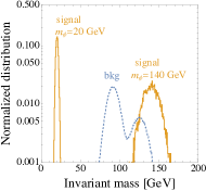
Figure 1: Invariant mass of the di-jet system after the basic cuts for the $\phi\to b\bar{b}$ channel. The blue curves represent the SM VBF $jj$ backgrounds, while the orange curves are the signal distributions for $m_{\phi}=20$ and 140 GeV.

The VBF $\phi\to\tau^{+}\tau^{-}$ and $b\bar{b}$ channels share the same main background: the SM VBF production of di-jet from photon splitting or $V$ and $h$ decays. We require both the signal and background events to have exactly two jets and no charged leptons with transverse momentum and pseudo-rapidity

$$p_{T}>30~{}{\rm GeV},\quad|\eta|<2.43,$$ (19)

and recoil mass

$$m_{\rm recoil}^{jj}=\sqrt{\left(p_{\mu^{+}}+p_{\mu^{-}}-p_{j_{1}}-p_{j_{2}}\right)^{2}}>200~{}{\rm GeV}.$$ (20)

The cut on $\eta$ corresponds to a detector angle coverage of $[10^{\circ},170^{\circ}]$. The event distributions of the di-jet invariant mass $m_{jj}$ in the $\phi\to b\bar{b}$ channel after basic cuts are displayed in Fig. 1, where the blue curve clearly shows the peaks of $m_{V,h}$ of the background, while the two orange curves demonstrate the signal peaks for $m_{\phi}=20$ and 140 GeV. A mass-shell cut

$$|m_{jj}-m_{\phi}|<{\rm min}\{0.2m_{\phi},~{}30~{}{\rm GeV}\},$$ (21)

can efficiently select signal agains the backgrounds, as illustrated in the cut flow of Table 1. We do not assume $b$-tagging in this simulation, but have checked that a 70% tagging rate yields similar results. For the $\tau^{+}\tau^{-}$ channel, we have included the tau hadronic decay branching ratio $\sim 65\%$ and assumed a $90\%$ tagging rate.

Cross sections [fb]	$\sigma_{S}^{20}$	$\sigma^{140}_{S}$	$\sigma_{B}$
No Cut	8.64	4.58	2870
Basic cuts	2.87	2.34	1366
Mass-shell cut, 20	2.85		0.207
Mass-shell cut, 140		2.33	343

Table 1: Cut flows for the $\phi\to b\bar{b}$ channel with $m_{\phi}=$ 20, 140 GeV and the backgrounds. For the signals, we assume $\sin\theta=0.1$.

In the VBF $\phi\to VV\to jjjj$ channel, the main background is the SM VBF $jjjj$ from pure EW process or involving QCD gluon splitting. We apply the following basic cuts: exactly four jets and no charged leptons within the kinetic region of Eq. (19), and the recoil mass

$$m_{\rm recoil}^{4j}=\sqrt{\left(p_{\mu^{+}}+p_{\mu^{-}}-\sum_{n=1}^{4}p_{j_{n}}\right)^{2}}>200~{}{\rm GeV}.$$ (22)

Then we pair the four jets by minimizing

$$\chi^{2}={\rm min}\left\{\frac{(m_{j_{1}j_{2}}-m_{W})^{2}}{\Gamma_{W}^{2}}+\frac{(m_{j_{3}j_{4}}-m_{W})^{2}}{\Gamma_{W}^{2}},\right.\\ \left.~{}\frac{(m_{j_{1}j_{2}}-m_{Z})^{2}}{\Gamma_{Z}^{2}}+\frac{(m_{j_{3}j_{4}}-m_{Z})^{2}}{\Gamma_{Z}^{2}}\right\},$$ (23)

where $\Gamma_{W,Z}$ are respectively the decay widths of the $W^{\pm}$ or $Z$ bosons. After pairing, $(j_{1}j_{2})$ and $(j_{3}j_{4})$ are identified as two $V$ candidates, as illustrated in blue peaked curves of Fig. 2. Note that the main background, the SM EW VBF production of $jjjj$, also has a peak at $\sim m_{V}$. However, the invariant mass of the entire $4j$ system peaks at $m_{\phi}$ for the signal, while the background has a mainly smooth distribution plus a small peak at $\sim m_{h}$ from the $h\to WW^{*}/ZZ^{*}$ decay, as shown in the orange curves. Therefore, the mass-shell cuts

$$|m_{j_{1}j_{2}}-m_{V}|<15~{}{\rm GeV},\quad|m_{j_{3},j_{4}}-m_{V}|<15~{}{\rm GeV}$$ (24)

for the $V$ candidates and

$$|m_{4j}-m_{\phi}|<30~{}{\rm GeV}$$ (25)

for the $4j$ system can efficiently remove background events and manifest the signal, as illustrated in Table 2.

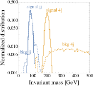
Figure 2: Invariant mass of the $jj$ (blue) and $4j$ (orange) systems after the basic cuts for the $\phi\to VV\to jjjj$ channel. The dashed curves represent the SM VBF $jjjj$ backgrounds, while the solid curves are the signal distributions for $m_{\phi}=200$ GeV.

Cross sections [fb]	$\sigma_{S}^{200}$	$\sigma_{B}^{\rm EW}$	$\sigma_{B}^{\rm QCD}$
No Cut	3.09	157	26.7
Basic cuts	0.481	39.7	5.41
Mass-shell cut for $V$	0.395	23.8	0.0615
Mass-shell cut for $\phi$	0.394	1.69	0.0246

Table 2: Cut flows for the $\phi\to VV$ channel with $m_{\phi}=200$ GeV and the backgrounds. For the signal, we assume $\sin\theta=0.1$.

For $m_{\phi}>2m_{h}$, the $\phi\to hh\to b\bar{b}b\bar{b}$ channel is the most effective probe of the model, with the main background being the SM VBF $jjjj$. We utilize the simulation results from Ref. Liu and Xie (2021), which is based on the xSM and is not for classically conformal models; however, the technical considerations are the same with our model for this specific channel.

IV Cosmological implications

While particle experiments effectively probe the excitations of the quantum field near the vacuum, the signals cannot be considered definitive evidence for the radiative EWSB mechanism. The phenomenology discussed in Section III primarily addresses a new scalar boson mixing with the Higgs boson, a prediction shared by many new physics models. In this section, we focus on the distinctive feature of the radiative EWSB mechanism: the logarithmic shape of the $\phi$-direction potential. We will demonstrate this shape leads to one or more FOPTs during cosmic evolution, resulting in GW signals.

IV.1 Thermal history

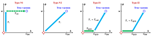
Figure 3: The field space trajectories of the possible cosmological thermal history. Type-N1: a conformal FOPT at $T_{*}$ followed by an EW crossover at $T_{\rm ew}$. Type-N2: a joint conformal-EW FOPT at $T_{*}$. Type-I1: a QCD-EW FOPT at $T_{\rm QCD}$ followed by a conformal FOPT at $T_{*}\approx T_{\rm roll}$. Type-I2: a joint QCD-EW-conformal FOPT at $T_{*}=T_{\rm QCD}$.

The scalar potential is modified by the dense and hot plasma of the early Universe to be

$$V_{T}(h,\phi,T)=V_{1}(h,\phi)+V_{T}^{\text{1-loop}}(h,\phi,T)\\ +V_{\rm daisy}(h,\phi,T),$$ (26)

where $T$ is the temperature, $V_{T}^{\text{1-loop}}$ is the one-loop thermal correction, and $V_{\rm daisy}$ is the daisy resummation. The full expression is given in Appendix A and included in our numerical calculation. For a quick qualitative understanding of cosmic history, we use the analytical approximation

$$V_{T}(h,\phi,T)\approx V_{1}(h,\phi)+\frac{c_{\phi}T^{2}}{2}\phi^{2}+\frac{c_{h}T^{2}}{2}h^{2},$$ (27)

where the coefficient

$$c_{h}=\frac{3g^{2}+g^{\prime 2}}{16}+\frac{y_{t}^{2}}{4}+\frac{\lambda_{h}}{2}\approx 0.4$$ (28)

is caused by the SM particles, and

$$c_{\phi}=\begin{dcases}\frac{g_{X}^{2}}{4},&\text{for the gauge-induced scenario;}\\ \frac{\lambda_{X}}{24},&\text{for the scalar-induced scenario,}\end{dcases}$$ (29)

is the BSM thermal correction. If after inflationary reheating $T\gg w$, the $T^{2}$-terms dominates Eq. (27), placing the vacuum at the origin of field space $(h,\phi)=(0,0)$, leading to symmetry restoration.

As the Universe cools, the vacuum of $V_{T}(h,\phi,T)$ eventually transitions to the zero-temperature position $(v,w)$. A notable feature arises from the logarithmic shape of the zero-temperature potential $V_{1}(h,\phi)$: it is flat near the origin, with all first- and second-order derivatives vanishing. Consequently, as long as $T>0$, the $T^{2}$-terms induce a local minimum for $V_{T}(h,\phi,T)$ at the origin. This indicates that the vacuum transition from $(0,0)$ at high temperatures to $(v,w)$ at zero temperature is not a smooth roll but rather a quantum tunneling process. At a specific temperature $T_{*}$, $V_{T}(h,\phi,T_{*})$ has two minima: the old vacuum $(0,0)$ and a new non-origin vacuum $(v_{*},w_{*})$, with the latter being the global minimum to which the Universe decays. This constitutes the cosmic FOPT, during which true vacuum bubbles nucleate, expand, and ultimately fill the entire Universe. After the FOPT, $(v_{*},w_{*})$ smoothly shifts to $(v,w)$ as $T\to 0$.

Below the critical temperature $T_{c}$, the non-origin minimum becomes the global minimum (true vacuum), and the decay rate per unit volume is Linde (1983)

$$\Gamma(T)\sim T^{4}\left(\frac{S_{3}}{2\pi T}\right)^{3/2}e^{-S_{3}/T},$$ (30)

where $S_{3}/T$ is the action of $O(3)$-symmetric bounce solution. The false vacuum fraction of the Universe is $p(T)=e^{-I(T)}$, with Guth and Tye (1980); Guth and Weinberg (1981)

$$I(T)=\frac{4\pi}{3}\int_{T}^{T_{c}}\frac{\Gamma(T^{\prime})\text{d}T^{\prime}}{T^{\prime 4}H(T^{\prime})}\left[\int_{T}^{T^{\prime}}\frac{v_{w}\text{d}T^{\prime\prime}}{H(T^{\prime\prime})}\right]^{3},$$ (31)

where $v_{w}$ is the bubble wall expansion velocity, and $H(T)$ is the Hubble constant. As the FOPT progresses, $p(T)\to 0$, and the true vacuum bubbles fulfill the space. The percolation temperature $T_{*}$ is defined at bubbles forming an infinite connected cluster, occurring at $p(T^{*})=0.71$ Rintoul and Torquato (1997).

FOPTs in radiative symmetry breaking (i.e., classically conformal) theories have garnered significant attention Huang and Xie (2022); Chun et al. (2023); Hambye and Strumia (2013); Hambye et al. (2018); Baldes and Garcia-Cely (2019); Yaser Ayazi and Mohamadnejad (2019); Mohamadnejad (2020); Khoze and Milne (2023); Frandsen et al. (2023); Wong and Xie (2023); Gouttenoire (2024); Salvio (2024, 2023); Conaci et al. (2024); Banerjee et al. (2024); Witten (1981); Konstandin and Servant (2011); Jinno and Takimoto (2017); Iso et al. (2017); Marzo et al. (2019); Bian et al. (2021); Ellis et al. (2019a, 2020); Jung and Kawana (2022); Kawana (2022); Sagunski et al. (2023); Ahriche et al. (2024). This topic is particularly important because the FOPTs are in general ultra-supercooled with $T_{*}\ll w$, significantly impacting cosmological history. For instance, in the gauge-induced scenario, $S_{3}/T\propto g_{X}^{-3}$ Iso et al. (2017), thus $\Gamma(T)\propto e^{-S_{3}/T}$ is strongly suppressed for small $g_{X}$. Consequently, FOPTs may occur at very late times, resulting in supercooling. Depending on the FOPT details, the evolution path of the Universe can be categorized into two main types, each with two variations, leading to four distinct possibilities.

Let $T_{\rm QCD}\approx 85$ MeV be a characteristic QCD temperature (to be explained later). When the conformal symmetry breaking FOPT occurs at $T_{*}>T_{\rm QCD}$, this is termed the normal pattern history. After the transition, $\phi\approx w$, and Eq. (27) reduces to

$$V_{T}(h,w,T)\approx\frac{1}{2}\left(c_{h}T^{2}-\frac{m_{h}^{2}}{2}\right)h^{2}+\frac{\lambda_{h}}{4}h^{4}.$$ (32)

The sign of the coefficient of $h^{2}$ in this potential depends on the hierarchy between $T_{*}$ and $T_{\rm ew}=m_{h}/\sqrt{2c_{h}}\approx 140$ GeV, classifying two sub-types of evolution possibilities.

1. Type-N1, $T_{*}>T_{\rm ew}$. The EW symmetry remains preserved after the conformal FOPT. An EW crossover occurs at $T_{\rm ew}$ where $h$ shifts smoothly to $v$.

2. Type-N2, $T_{*}<T_{\rm ew}$. The EWSB simultaneously occurs with the conformal FOPT, resulting in a joint conformal-EW FOPT at $T_{*}$.

If the decay rate is sufficiently low for the Universe to remain at $(0,0)$ until $T_{\rm QCD}$, then the QCD phase transition occurs first, a scenario we call inverted pattern history. In this case, the QCD phase transition takes place with six-flavor massless quarks, resulting in a FOPT Braun and Gies (2006); Pisarski and Wilczek (1984); Guan and Matsuzaki (2024), as opposed to a crossover in the SM thermal history. The QCD also triggers an EW FOPT from $h=0$ to $v_{\rm QCD}\approx 100$ MeV via the top quark condensate and Yukawa interaction $-y_{t}h\left\langle\bar{t}t\right\rangle/\sqrt{2}$ Witten (1981); Iso et al. (2017). After this joint QCD-EW FOPT, $h\approx v_{\rm QCD}$, and Eq. (27) simplifies to

$$V_{T}(v_{\rm QCD},\phi,T)\approx\frac{1}{2}\left(c_{\phi}T^{2}-\frac{m_{h}^{2}v_{\rm QCD}^{2}}{2w^{2}}\right)\phi^{2}\\ +\frac{B}{4}\phi^{4}\left(\log\frac{\phi}{w}-\frac{1}{4}\right).$$ (33)

The sign of the coefficient $\phi^{2}$ depends on the hierarchy between $T_{\rm QCD}$ and $T_{\rm roll}=m_{h}v_{\rm QCD}/(\sqrt{2c_{\phi}}w)$, classifying two sub-types of evolution possibilities.

1. Type-I1, $T_{\rm QCD}>T_{\rm roll}$. After the QCD-EW FOPT, a $\phi$-direction FOPT occurs at $T_{*}\approx T_{\rm roll}$, which also induces the transition of $h$ from $v_{\rm QCD}$ to $\sim v$.

2. Type-I2, $T_{\rm QCD}<T_{\rm roll}$. The $\phi$-direction also gains a VEV at QCD-EW FOPT, thus this is in fact a joint QCD-EW-conformal FOPT at $T_{*}=T_{\rm QCD}$.

The field evolution trajectories of the four thermal history patterns are sketched in Fig. 3. The existence of the inverted pattern was proposed and studied in Refs. Witten (1981); Iso et al. (2017), while Type-I2 has been discussed in detail using low-energy QCD effective models Sagunski et al. (2023).

It is important to note that reheating after the FOPT is not included in this discussion for simplicity. Supercooled FOPTs release a significant amount of vacuum energy into the plasma, reheating the Universe to a temperature $T_{\rm rh}\geqslant T_{*}$. The cosmic history is further complicated if $T_{\rm rh}\gg T_{*}$. For example, if $T_{*}<T_{\rm ew}<T_{\rm rh}$, the evolution is a Type-N2 trajectory followed by the EW symmetry restoration at $T_{\rm rh}$, and then an EW crossover at $T_{\rm ew}$.

IV.2 FOPT dynamics and GW detection

In this research, we focus on the case of $w\gg v$ and hence $|\lambda_{h\phi}|\ll 1$. Consequently, the FOPT dynamics of the $\phi$-direction can be treated separately from the SM sector, and we adopt the $\phi$-dependent thermal potential as

$$V_{T}(\phi,T)\approx V_{T}(0,\phi,T)+V_{\rm QCD}(\phi,T),$$ (34)

where

$$\delta V_{\rm QCD}(\phi,T)=\begin{dcases}~{}0,&T>T_{\rm QCD};\\ ~{}-\frac{m_{h}^{2}v_{\rm QCD}^{2}}{4w^{2}}\phi^{2},&T<T_{\rm QCD},\end{dcases}$$ (35)

is added to mimic the effect of the QCD-EW FOPT. This approach allows us to calculate the four thermal history patterns, except for Type-I2, which requires a detailed treatment of the QCD transition Sagunski et al. (2023). Fortunately, the parameter space of interest primarily involves Types-N1, N2, and I1, making this method sufficient for our analysis.

To calculate $\Gamma(T)$, one needs to evaluate the $O(3)$-symmetric bounce $\phi(r)$ solution by solving

$$\frac{\text{d}^{2}\phi}{\text{d}r^{2}}+\frac{2}{r}\frac{\text{d}\phi}{\text{d}r}=\frac{\text{d}V_{T}}{\text{d}\phi},\quad\frac{\text{d}\phi}{\text{d}r}\Big{|}_{r=0}=0,\quad\lim_{r\to\infty}\phi=0,$$ (36)

where the Euclidean action is

$$\frac{S_{3}}{T}=\frac{1}{T}\int_{0}^{\infty}4\pi r^{2}\text{d}r\left[\frac{1}{2}\left(\frac{\text{d}\phi}{\text{d}r}\right)^{2}+V_{T}\left(\phi(r),T\right)\right].$$ (37)

After determining $\Gamma(T)$, we derive $p(T)$ and resolve $T_{*}$ assuming $v_{w}\approx 1$. If $T_{*}>T_{\rm QCD}$ and the FOPT completion condition Ellis et al. (2019b); Turner et al. (1992)

$$3+T_{*}\frac{\text{d}I}{\text{d}T}\Big{|}_{T_{*}}<0$$ (38)

is satisfied, ensuring that the physical volume of the false vacuum is still decreasing at percolation, this corresponds to the normal pattern. Conversely, if $T_{*}<T_{\rm QCD}$, then the QCD-EW FOPT occurs, indicating the inverted pattern. We have developed and optimized homemade codes to solve Eq. (36) for $T\ll w$.

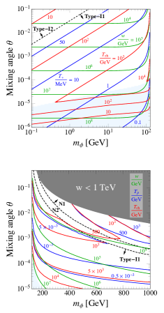
Figure 4: Contours of $w$ (green) and FOPT characteristic temperatures $T_{*}$ (blue) and $T_{\rm rh}$ (red) for the gauge-induced scenario. The black dashed lines are the boundaries of different thermal history patterns, and the light blue shaded regions correspond to slow reheating. The top (bottom) panel is for the $m_{\phi}<m_{h}$ ($m_{\phi}>m_{h}$) case.

The reheating temperature following the FOPT is Hambye et al. (2018)

$$T_{\rm rh}={\rm max}\left\{T_{*},~{}T_{\Lambda}\times{\rm min}\left\{1,~{}\frac{\Gamma_{s}}{H(T_{*})}\right\}\right\},$$ (39)

where $\Gamma_{s}=\Gamma_{h}\sin^{2}\theta+\Gamma_{\phi}\cos^{2}\theta$ with $\Gamma_{h}$ and $\Gamma_{\phi}$ being the decay width of the $h$ and $\phi$ bosons, respectively, and $T_{\Lambda}$ is the temperature of vacuum-radiation equality defined by

$$\frac{\pi^{2}}{30}g_{*}(T_{\Lambda})T_{\Lambda}^{4}=\Delta V_{T}(T_{\Lambda}),$$ (40)

with $g_{*}$ the effective degrees of freedom, and $\Delta V_{T}(T)$ the vacuum energy difference between the false and true vacua at $T$. If $\Gamma_{s}\gtrsim H(T_{*})$, the reheating is instant, and $T_{\rm rh}=T_{\Lambda}$.

We analyze the parameter space of the gauge-induced radiative symmetry breaking scenario, scan over $(m_{\phi},\theta)$ and plot the contours of $w$ (green), $T_{*}$ (blue), and $T_{\rm rh}$ (red) in Fig. 4 (similar results for the scalar-induced scenario are obtained). Due to the non-degeneracy between $\phi$ and $h$, we display the regions where $m_{\phi}<m_{h}$ in the top panel and $m_{\phi}>m_{h}$ in the bottom panel. The boundaries of different thermal history patterns are delineated with black dashed lines. In the case of light $\phi$, we only observe inverted patterns. Here, the conformal FOPT occurs at a low temperature, approximately $T_{*}\sim\mathcal{O}(0.1-100)~{}{\rm MeV}$, followed by reheating to $T_{\rm rh}\sim\mathcal{O}(10-10^{4})~{}{\rm GeV}\gg T_{*}$. A region of slow reheating (i.e. $\Gamma_{s}<H(T_{*})$) is identified for $\theta\lesssim 10^{-5}$ by a light blue shaded area.

For heavy $\phi$, both normal and inverted patterns are possible, and only a narrow region in the lower-left corner exhibits slow reheating. When the FOPT reheating is prompt, $T_{\rm rh}\approx\max\{T_{*},T_{\Lambda}\}$. Therefore, when supercooling is not prominent, FOPT completes during the radiation era, yielding $T_{*}\approx T_{\rm rh}$, which leads to the overlap of the $10^{3}$ GeV red and blue contours. As $m_{\phi}$ is fixed and $\theta$ decreases, supercooling is enhanced, resulting in a decrease in $T_{*}$ and an increase in $T_{\Lambda}$. Consequently, $T_{\rm rh}$ initially decreases before increasing, producing a cusp-shaped red contour around 500 GeV. In the inverted pattern region, $T_{\rm rh}\gg T_{*}$, significant reheating is obtained.

If $T_{*}<T_{\Lambda}$, the Universe enters a vacuum domination era before the FOPT, known as thermal inflation Lyth and Stewart (1996). On the other hand, if reheating after the FOPT is slow such that $T_{\rm rh}<T_{\Lambda}$, the Universe undergoes a matter domination era after the FOPT Dutra and Wu (2023). These varied thermal history scenarios encompassing the four previously classified patterns provide a special and interesting spacetime background for addressing the longstanding puzzles in particle physics and cosmology, including generating the baryon asymmetry Huang and Xie (2022); Chun et al. (2023) and forming dark matter Hambye and Strumia (2013); Hambye et al. (2018); Baldes and Garcia-Cely (2019); Yaser Ayazi and Mohamadnejad (2019); Mohamadnejad (2020); Khoze and Milne (2023); Frandsen et al. (2023); Wong and Xie (2023) or even sourcing primordial black holes Gouttenoire (2024); Salvio (2024, 2023); Conaci et al. (2024); Banerjee et al. (2024).

In this research, we focus solely on the stochastic GWs generated by the FOPT. There are three main sources of the GWs: bubble collisions, sound waves, and turbulence, with their relative strengths depending on the energy budget of the transition Espinosa et al. (2010); Ellis et al. (2019a, 2020); Giese et al. (2020); Wang and Yuwen (2022). If bubble walls are still in accelerating expansion at $T_{*}$, most of the FOPT energy is stored in the walls, leading to dominance by bubble collisions. However, if the bubble walls reach terminal velocity before percolation, the energy is primarily released to bulk motion, making sound waves the primary source. The energy budget can be evaluated by analyzing the motion of the walls, involving competition between vacuum pressure $\Delta V_{T}$ and the frictional force $\mathcal{P}$ from particle transitions across the wall. Different results are obtained Ellis et al. (2019a, 2020) for varying scaling of the resummed $(1\to n)$-splitting-induced friction, either $\propto\gamma_{w}$ Bodeker and Moore (2017); Gouttenoire et al. (2022) or $\propto\gamma_{w}^{2}$ Höche et al. (2021), where $\gamma_{w}=(1-v_{w}^{2})^{-1/2}$ . We apply both methods and find that the projected detectable reach is not sensitive to the chosen calculation method.

The GW spectrum is defined as the energy density fraction $\Omega_{\rm gw}(f)$, which can be expressed as numerical formulae in terms of $T_{*}$, $v_{w}$, and two more effective FOPT parameters: the ratio of latent heat to the radiation energy density

$$\alpha=\frac{1}{\pi^{2}g_{*}(T_{*})T_{*}^{4}/30}\left(\Delta V_{T}-T\frac{\text{d}\Delta V_{T}}{\text{d}T}\right)\Big{|}_{T_{*}},$$ (41)

characterizing the strength of the transition, with $\alpha>1$ implying thermal inflation; the ratio of Hubble time to the FOPT duration

$$\frac{\beta}{H_{*}}=T_{*}\frac{\text{d}}{\text{d}T}\left(\frac{S_{3}}{T}\right)\Big{|}_{T_{*}}.$$ (42)

In certain parameter space regions, the FOPT is very slow and we switch to use another definition Kanemura et al. (2024)

$$\frac{\beta}{H_{*}}\to\frac{(8\pi)^{1/3}v_{w}}{H_{*}\bar{R}},$$ (43)

where $\bar{R}$ is the mean separation of bubble Ellis et al. (2019b), which can be taken as $n_{b}^{-1/3}$, with $n_{b}$ being the bubble density Wang et al. (2020).

We derive $\alpha$ and $\beta/H_{*}$ at $T_{*}$ to get the GW spectra at the FOPT Huber and Konstandin (2008); Hindmarsh et al. (2015); Caprini et al. (2009), and assume that the shapes remain unchanged during the instant reheating from $T_{*}$ to $T_{\rm rh}$. We then redshift the spectra from $T_{\rm rh}$ to today $T_{0}\approx 2.73$ K Breitbach et al. (2019). Note that if $T_{\rm rh}\approx T_{*}$ then the treatment is equivalent to the numerical formulae in Refs. Caprini et al. (2016, 2020). However, in our scenario, usually $T_{\rm rh}\gg T_{*}$, thus the difference is significant. If the reheating is slow, $T_{\rm rh}\ll T_{\Lambda}$, the GW shape is further affected Ellis et al. (2020), but this is not a concern in the GW-detectable parameter space. The GW spectra today lie within the sensitivity region of the future space-based interferometer GW detectors such as LISA Amaro-Seoane et al. (2017), TianQin Luo et al. (2016), Taiji Hu and Wu (2017), and BBO Crowder and Cornish (2005).

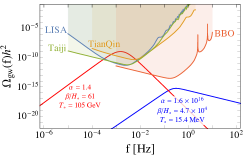
Figure 5: Illustrations of the GW spectra for $m_{\phi}=200$ GeV, $\theta=0.1$ ($w=1.6$ TeV and $g_{X}=0.79$, red curve) and $m_{\phi}=10$ GeV, $\theta=0.01$ ($w=25$ TeV and $g_{X}=0.046$, blue curve) in the gauge-induced scenario, with the FOPT parameters given in the figure.

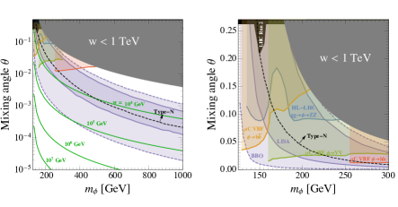
Figure 6: Current bounds and projected limits on the parameter space for the $m_{\phi}>m_{h}$ case, with the right panel being the zoomed-in figure of the left panel in the mass range $m_{\phi}\in[m_{h},~{}300~{}{\rm GeV}]$. The black shaded region is already excluded, while the colored shaded regions represent the reach of future experiments. The black dashed lines are the boundaries between normal and inverted thermal history patterns, while the green solid lines plot the contour of $w$.

Before presenting the projected reach in the next section, we briefly comment on the GW spectra in our model. Most parameter space reveals strong FOPTs with $\alpha\gg 1$. However, this doesn’t necessarily imply strong GWs. As noted in Ref. Kanemura et al. (2024), strong GWs require a transition that is both strong and slow, characterized by large $\alpha$ and small $\beta/H_{*}$. In our model, many regions allow for ultra-supercooled FOPTs with prolonged thermal inflation, greatly impacting cosmic history but resulting in rapid transitions that produce no detectable GWs. To illustrate, Fig. 5 shows the GW spectra for two benchmarks in the gauge-induced radiative symmetry breaking scenario. The red curve corresponds to a strong, slow transition with detectable signals for instruments like LISA; while the blue curve represents a super-strong but prompt transition, yielding signals too weak for detection, even though $\alpha\sim 10^{16}$ is extremely large.

V Results

Combining the discussions in Section III and Section IV, this section presents the main results of our research. Fig. 6 displays current bounds and projected limits for the heavy scalar case where $m_{\phi}>m_{h}$. The left panel shows a scan of $m_{\phi}$ over the range $[m_{h},~{}1~{}{\rm TeV}]$ (linear scale) and $\theta$ over $[10^{-6},~{}{0.5}]$ (log scale). The right panel provides a detailed view of the region $m_{\phi}\in[m_{h},~{}300~{}{\rm GeV}]$ and $\theta\in[0,~{}0.27]$ (double-linear scale). Due to the validity of our sequential symmetry breaking treatment for $w\gg v$, we exclude the parameter space where $w<1$ TeV with the gray shaded region.

The current bounds are derived from LHC Run 2 results on Higgs signal strength Aad et al. (2024) (combining $36.1~{}{\rm fb}^{-1}$ to $139~{}{\rm fb}^{-1}$) and BSM searches for $\phi\to ZZ$ Sirunyan et al. (2018) (with $35.9~{}{\rm fb}^{-1}$). The colored shaded regions indicate various future projections. The CMS $\phi\to ZZ$ result is rescaled to $3000~{}{\rm fb}^{-1}$ for the HL-LHC reach, which can achieve sensitivity of $\theta\sim 0.1$ for $m_{h}\lesssim m_{\phi}\lesssim 2m_{h}$ when the $\phi\to ZZ^{(*)}$ branching ratio is significant. The reduced sensitivity around $m_{\phi}\sim 170$ GeV is due to the suppression of the branching ratio Djouadi (2008). Additionally, projections for VBF $\phi\to b\bar{b}$, $VV$, and $hh$ channels at future 10 TeV muon colliders indicate sensitivities reaching $\theta\sim 10^{-2}$. The dominance of different channels across various mass ranges reflects the branching ratio characteristics described in Eq. (16).

We present projections for future GW detectors LISA Amaro-Seoane et al. (2017) and its proposed successor BBO Crowder and Cornish (2005). TianQin Luo et al. (2016) and Taiji Hu and Wu (2017) are expected to yield similar sensitivity with LISA. The detection limit is defined by requiring the signal-to-noise ratio

$${\rm SNR}=\sqrt{\mathcal{T}\int\text{d}f\left(\frac{\Omega_{\rm gw}(f)}{\Omega_{\rm detector}(f)}\right)^{2}}=50,$$ (44)

using the sensitivity curves $\Omega_{\rm detector}(f)$ of LISA and BBO from Ref. Schmitz (2021), and the operational time is approximately $\mathcal{T}\approx 9.46\times 10^{7}~{}{\rm s}=0.75\times 4$ years Caprini et al. (2020). The projected region for GW detection is significantly larger than that for colliders in the log-$\theta$ coordinate perspective, with LISA probing $\theta$ down to $10^{-4}$ and BBO down to $10^{-5}$, and $w$ up to $10^{4}$ GeV and $10^{5}$ GeV, respectively.

While the collider reach is independent of the origin of radiative symmetry breaking, the dynamics of FOPT does depend on the origin of the parameter $B$. Consequently, gauge- and scalar-induced scenarios yield different GW spectra for a given parameter point $(m_{\phi},\theta)$, and here we show the results for the former scenario. However, we find that the projected reach of $\theta$ for a given $m_{\phi}$ varies by less than a factor of 2, which is negligible compared to the uncertainties in FOPT GW calculations Athron et al. (2024); Guo et al. (2021). Therefore, the probed region in Fig. 6 is insensitive to the origin of $B$. Henceforth, we will use the gauge-induced scenario as our primary example.

The left panel of Fig. 6 illustrates that GW and collider searches are complementary across most of the parameter space. The right panel zooms in on the region where these searches overlap, allowing for crosscheck. A future GW excess detected by LISA, TianQin, Taiji, or BBO could be further validated by signals from the HL-LHC or muon collider, supporting its origin as a FOPT via the radiative symmetry breaking mechanism. As shown in the figure, the $\phi\to hh$ channel covers only a small portion of the GW detection region, whereas the $\phi\to b\bar{b}$ and $\phi\to VV$ channels provide significant contributions for verifying GW detection. This is different from the xSM, where the majority of the GW detectable parameter space can be probed by the $\phi\to hh$ channel at the 10 TeV muon collider Liu and Xie (2021) (see also Refs. Alves et al. (2018, 2020, 2021) for di-Higgs probes of xSM FOPTs).

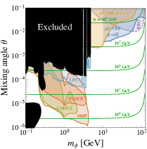
Figure 7: Current bounds and projected limits on the parameter space for the $m_{\phi}<m_{h}$ case. The black shaded region is already excluded, while the colored shaded regions represent the reach of future experiments. The green solid lines plot the contour of $w$.

The combined results for the $m_{\phi}<m_{h}$ case are shown in Fig. 7, where the black region is excluded, and the colored shaded areas indicate future projections. The green solid lines represent contours of $w$. Current bounds arise from various collider and beam-dump experiments that search for a light scalar boson mixing with the Higgs boson, including LHCb Aaij et al. (2017, 2015), NA62 Cortina Gil et al. (2021a, b), CHARM Winkler (2019), E949 Artamonov et al. (2009), LSND Foroughi-Abari and Ritz (2020), and MicroBooNE Abratenko et al. (2021). The constraint from SN1987 is illustrated as a separate shaded region in the bottom-left corner Winkler (2019). We also show the projected reach for $m_{\phi}\lesssim 2m_{\tau}$ from the LLP searches in LHCb, FASER Ariga et al. (2019), CODEX Gligorov et al. (2018), and SHiP Ahdida et al. (2021) based on results from Refs. Feng et al. (2018); Kling and Trojanowski (2021). These future experiments can probe $\theta$ as low as $10^{-6}$ with $w$ reaching up to $10^{8}$ GeV.

The prompt decay of $\phi\to\tau^{+}\tau^{-}$ and $b\bar{b}$ can probe $m_{\phi}\gtrsim 2m_{\tau}$ with $\theta$ reaching a few $10^{-3}$. Notably, this region can be crosschecked by signals detected by BBO. As shown in Fig. 4 of Section IV, the $m_{\phi}<m_{h}$ case corresponds to an inverted thermal history where the conformal phase transition is delayed until after the QCD-EW FOPT. The Type-I2 region is in the top-left part of the figure and excluded by existing data, leaving the viable type-I1 region, where a $\phi$-direction FOPT occurs at $T_{*}\approx T_{\text{roll}}<T_{\rm QCD}$. While such a FOPT can be extremely strong, with $\alpha$ reaching up to $10^{30}$, the duration of the transition is very short, yielding $\beta/H_{*}$ up to $10^{9}$. As a result, the GWs produced are weak, and only BBO can explore a small fraction of the parameter space in the top-right corner of the figure. This counterintuitive result arises because, following the QCD-EW FOPT, a negative mass squared term Eq. (35) is induced along the $\phi$-direction, causing the local minimum of $\phi=0$ to disappear at $T_{\rm roll}$ and resulting in a rapid transition.

We note that Higgs exotic decay $h\to\phi\phi$ is not sensitive to the radiative symmetry breaking mechanism, as the branching ratio $\lesssim 10^{-10}$ in the $m_{\phi}<m_{h}/2$ region of Fig. 7. This suppression comes from the $m_{\phi}^{2}/w^{2}$ factor in the coefficient of the $h\phi^{2}$ term in Eq. (15). This behavior is a characteristic of the radiative symmetry breaking scenario and contrasts significantly with non-conformal extensions of the SM, such as the $U(1)^{\prime}$-extension or xSM, where Higgs exotic decays can effectively probe FOPTs Li and Xie (2023); Carena et al. (2023); Kozaczuk et al. (2020); Carena et al. (2020); Liu et al. (2022a); Kanemura and Li (2024).

VI Conclusion

We have presented a detailed phenomenological analysis of radiative EWSB, focusing on its key feature: the logarithmic potential. Excitations of the field quanta around the vacuum yield a new scalar particle, which can be investigated at particle colliders or beam-dump experiments. Moreover, the flat potential near the origin can induce one or more FOPTs during cosmic evolution, generating stochastic GW detectable by space-based interferometers. Following a detailed analysis of the vacuum structure of the joint scalar potential, the experimental signals are studied. In collider studies, we analyze LLP signals and the prompt decay of the new scalar into SM particle pairs. On the cosmological side, we investigate FOPT dynamics, classifying four distinct thermal history patterns (with further variations due to reheating effects), and subsequently calculate the resulting GWs.

The combined results from particle and GW experiments effectively probe the parameter space, revealing both complementary and overlapping regions. For the case $m_{\phi}<m_{h}$, future LLP searches offer the most sensitive exploration of the mechanism, reaching scales up to $w\sim 10^{8}$ GeV. For $m_{\phi}>m_{h}$, GWs from FOPTs can probe $w$ up to $10^{5}$ GeV at the BBO. In both scenarios, there is overlap region between collider and GW experiments, enabling crosschecks that can help identify the radiative symmetry breaking mechanism. Remarkably, the $\tau^{+}\tau^{-}$, $b\bar{b}$, $VV$, and $hh$ channels all significantly contribute to the cross-verification of GW detections, in contrast to the $hh$-dominance observed in the non-conformal xSM case.

Utilizing the diverse thermal history patterns identified, novel solutions can be proposed to BSM puzzles in particle physics and cosmology. For instance, dark matter or baryon asymmetry may be generated via particle interactions with ultra-relativistic bubble walls Huang and Xie (2022); Chun et al. (2023) or after thermal inflation Hambye et al. (2018); Baldes and Garcia-Cely (2019); Wong and Xie (2023). Slow transition may form primordial black holes through false vacuum islands Gouttenoire (2024); Salvio (2024, 2023); Conaci et al. (2024); Banerjee et al. (2024). See Refs. Baldes et al. (2021); Azatov et al. (2021a, b); Baldes et al. (2023); Ai et al. (2024); Liu et al. (2022b); Cai et al. (2024) for more relevant studies based on the general supercooled FOPTs, which naturally apply to radiative symmetry breaking models. Our work can thus serve as a foundation for these further investigations.

Appendix A Detailed expressions of the thermal potential

The one-loop thermal term is given by

$$V_{T}^{\text{1-loop}}(h,\phi,T)=\sum_{i}\frac{n_{i}T^{4}}{2\pi^{2}}J_{B/F}\left(\frac{M_{i}^{2}}{T^{2}}\right),$$ (45)

where the summation runs over particles whose mass depend on the background fields $h$ and $\phi$, and the thermal integrations are defined as

$$J_{B/F}(y)=\pm\int_{0}^{\infty}x^{2}{\rm d}x\ln\left(1\mp e^{-\sqrt{x^{2}+y}}\right),$$ (46)

with the subscript $B$ and $F$ denoting bosonic and fermionic contribution, respectively. The field-dependent masses and numbers of effective degrees of freedom are

$$\begin{dcases}~{}M_{W}(h)=\frac{g}{2}h,&n_{W}=2\times 3=6;\\ ~{}M_{Z}(h)=\frac{\sqrt{g^{2}+g^{\prime 2}}}{2}h,&n_{Z}=3;\\ ~{}M_{t}(h)=\frac{y_{t}}{\sqrt{2}}h,&n_{t}=N_{c}\times 4=12,\end{dcases}$$ (47)

for the SM gauge bosons and top quark where $g$ and $g^{\prime}$ are the gauge couplings of the SM $SU(2)_{L}$ and $U(1)_{Y}$ groups, respectively, and $y_{t}$ is the top quark Yukawa. The SM scalars have

$$\begin{dcases}~{}M_{h}^{2}(h,\phi)=3\lambda_{h}h^{2}+\frac{\lambda_{h\phi}}{2}\phi^{2},&n_{h}=1;\\ M_{G}^{2}(h,\phi)=\lambda_{h}h^{2}+\frac{\lambda_{h\phi}}{2}\phi^{2},&n_{G}=3.\end{dcases}$$ (48)

The BSM sector has

$$M_{Z^{\prime}}(\phi)=g_{X}\phi,\quad n_{Z^{\prime}}=3,$$ (49)

for the gauge-induced scenario and

$$M_{X}(\phi)=\sqrt{\frac{\lambda_{X}}{2}}\phi,\quad n_{X}=1,$$ (50)

for the scalar-induced scenario.

The daisy resummation term can be decomposed as to the SM and BSM components, and the latter is

$$\begin{dcases}~{}-\frac{T}{12\pi}g_{X}^{3}\left[\left(\phi^{2}+T^{2}\right)^{3/2}-\phi^{3}\right],\\ ~{}-\frac{T}{12\pi}\left(\frac{\lambda_{X}}{2}\right)^{3/2}\left[\left(\phi^{2}+\frac{T^{2}}{12}\right)^{3/2}-\phi^{3}\right],\end{dcases}$$ (51)

for the gauge- and scalar-induced radiative symmetry breaking, respectively. The expression of the SM daisy resummation is involved and not crucial for our discussion, thus is not shown here, and we refer the readers to Ref. Carrington (1992) for the details.

The approximate potential Eq. (27) is obtained by expanding the thermal integrations around $y\approx 0$:

$$\begin{split}J_{B}(y)\approx&-\frac{\pi^{4}}{45}+\frac{\pi^{2}}{12}y-\frac{\pi}{6}y^{3/2}-\frac{y^{2}}{32}\log\frac{y}{a_{B}},\\ J_{F}(y)\approx&-\frac{7\pi^{4}}{360}+\frac{\pi^{2}}{24}y+\frac{y^{2}}{32}\log\frac{y}{a_{F}},\end{split}$$ (52)

where $a_{B}=16a_{F}$ and $a_{F}=\pi^{2}e^{1.5-2\gamma_{E}}$ with $\gamma_{E}\approx 0.577$ the Euler’s constant.

References

- Aad et al. (2012) G. Aad et al. (ATLAS), Phys. Lett. B 716, 1 (2012), eprint 1207.7214.
- Chatrchyan et al. (2012) S. Chatrchyan et al. (CMS), Phys. Lett. B 716, 30 (2012), eprint 1207.7235.
- Coleman and Weinberg (1973) S. R. Coleman and E. J. Weinberg, Phys. Rev. D 7, 1888 (1973).
- Jackiw (1974) R. Jackiw, Phys. Rev. D 9, 1686 (1974).
- Bardeen (1995) W. A. Bardeen, in Ontake Summer Institute on Particle Physics (1995).
- Meissner and Nicolai (2008) K. A. Meissner and H. Nicolai, Phys. Lett. B 660, 260 (2008), eprint 0710.2840.
- de Boer et al. (2024) T. de Boer, M. Lindner, and A. Trautner (2024), eprint 2407.15920.
- Frasca et al. (2024) M. Frasca, A. Ghoshal, and N. Okada (2024), eprint 2408.00093.
- Nakayama (2015) Y. Nakayama, Phys. Rept. 569, 1 (2015), eprint 1302.0884.
- Hempfling (1996) R. Hempfling, Phys. Lett. B 379, 153 (1996), eprint hep-ph/9604278.
- Iso et al. (2009a) S. Iso, N. Okada, and Y. Orikasa, Phys. Lett. B 676, 81 (2009a), eprint 0902.4050.
- Iso et al. (2009b) S. Iso, N. Okada, and Y. Orikasa, Phys. Rev. D 80, 115007 (2009b), eprint 0909.0128.
- Chun et al. (2013) E. J. Chun, S. Jung, and H. M. Lee, Phys. Lett. B 725, 158 (2013), [Erratum: Phys.Lett.B 730, 357–359 (2014)], eprint 1304.5815.
- Das et al. (2017) A. Das, N. Okada, and N. Papapietro, Eur. Phys. J. C 77, 122 (2017), eprint 1509.01466.
- Khoze and Ro (2013) V. V. Khoze and G. Ro, JHEP 10, 075 (2013), eprint 1307.3764.
- Davoudiasl and Lewis (2014) H. Davoudiasl and I. M. Lewis, Phys. Rev. D 90, 033003 (2014), eprint 1404.6260.
- Huang and Xie (2022) P. Huang and K.-P. Xie, JHEP 09, 052 (2022), eprint 2206.04691.
- Chun et al. (2023) E. J. Chun, T. P. Dutka, T. H. Jung, X. Nagels, and M. Vanvlasselaer, JHEP 09, 164 (2023), eprint 2305.10759.
- Okada and Orikasa (2012) N. Okada and Y. Orikasa, Phys. Rev. D 85, 115006 (2012), eprint 1202.1405.
- Hambye and Strumia (2013) T. Hambye and A. Strumia, Phys. Rev. D 88, 055022 (2013), eprint 1306.2329.
- Hambye et al. (2018) T. Hambye, A. Strumia, and D. Teresi, JHEP 08, 188 (2018), eprint 1805.01473.
- Baldes and Garcia-Cely (2019) I. Baldes and C. Garcia-Cely, JHEP 05, 190 (2019), eprint 1809.01198.
- Yaser Ayazi and Mohamadnejad (2019) S. Yaser Ayazi and A. Mohamadnejad, JHEP 03, 181 (2019), eprint 1901.04168.
- Mohamadnejad (2020) A. Mohamadnejad, Eur. Phys. J. C 80, 197 (2020), eprint 1907.08899.
- Khoze and Milne (2023) V. V. Khoze and D. L. Milne, Phys. Rev. D 107, 095012 (2023), eprint 2212.04784.
- Frandsen et al. (2023) M. T. Frandsen, M. Heikinheimo, M. E. Thing, K. Tuominen, and M. Rosenlyst, Phys. Rev. D 108, 015033 (2023), eprint 2301.00041.
- Wong and Xie (2023) X.-R. Wong and K.-P. Xie, Phys. Rev. D 108, 055035 (2023), eprint 2304.00908.
- Gouttenoire (2024) Y. Gouttenoire, Phys. Lett. B 855, 138800 (2024), eprint 2311.13640.
- Salvio (2024) A. Salvio, Phys. Lett. B 852, 138639 (2024), eprint 2312.04628.
- Salvio (2023) A. Salvio, JCAP 12, 046 (2023), eprint 2307.04694.
- Conaci et al. (2024) A. Conaci, L. Delle Rose, P. S. B. Dev, and A. Ghoshal (2024), eprint 2401.09411.
- Banerjee et al. (2024) I. K. Banerjee, U. K. Dey, and S. Khalil (2024), eprint 2406.12518.
- Gildener and Weinberg (1976) E. Gildener and S. Weinberg, Phys. Rev. D 13, 3333 (1976).
- Chataignier et al. (2018) L. Chataignier, T. Prokopec, M. G. Schmidt, and B. Świeżewska, JHEP 08, 083 (2018), eprint 1805.09292.
- Lewis and Sullivan (2017) I. M. Lewis and M. Sullivan, Phys. Rev. D 96, 035037 (2017), eprint 1701.08774.
- Liu and Xie (2021) W. Liu and K.-P. Xie, JHEP 04, 015 (2021), eprint 2101.10469.
- Li and Xie (2023) S.-P. Li and K.-P. Xie, Phys. Rev. D 108, 055018 (2023), eprint 2307.01086.
- Gershtein et al. (2021) Y. Gershtein, S. Knapen, and D. Redigolo, Phys. Lett. B 823, 136758 (2021), eprint 2012.07864.
- Djouadi (2008) A. Djouadi, Phys. Rept. 457, 1 (2008), eprint hep-ph/0503172.
- Batell et al. (2022) B. Batell, N. Blinov, C. Hearty, and R. McGehee, in Snowmass 2021 (2022), eprint 2207.06905.
- Anastasiou et al. (2016) C. Anastasiou, C. Duhr, F. Dulat, E. Furlan, T. Gehrmann, F. Herzog, A. Lazopoulos, and B. Mistlberger, JHEP 09, 037 (2016), eprint 1605.05761.
- Sirunyan et al. (2018) A. M. Sirunyan et al. (CMS), JHEP 06, 127 (2018), [Erratum: JHEP 03, 128 (2019)], eprint 1804.01939.
- Delahaye et al. (2019) J. P. Delahaye, M. Diemoz, K. Long, B. Mansoulié, N. Pastrone, L. Rivkin, D. Schulte, A. Skrinsky, and A. Wulzer (2019), eprint 1901.06150.
- Aime et al. (2022) C. Aime et al. (2022), eprint 2203.07256.
- Accettura et al. (2023) C. Accettura et al., Eur. Phys. J. C 83, 864 (2023), [Erratum: Eur.Phys.J.C 84, 36 (2024)], eprint 2303.08533.
- Han et al. (2021) T. Han, Y. Ma, and K. Xie, Phys. Rev. D 103, L031301 (2021), eprint 2007.14300.
- Alloul et al. (2014) A. Alloul, N. D. Christensen, C. Degrande, C. Duhr, and B. Fuks, Comput. Phys. Commun. 185, 2250 (2014), eprint 1310.1921.
- Alwall et al. (2014) J. Alwall, R. Frederix, S. Frixione, V. Hirschi, F. Maltoni, O. Mattelaer, H. S. Shao, T. Stelzer, P. Torrielli, and M. Zaro, JHEP 07, 079 (2014), eprint 1405.0301.
- Linde (1983) A. D. Linde, Nucl. Phys. B 216, 421 (1983), [Erratum: Nucl.Phys.B 223, 544 (1983)].
- Guth and Tye (1980) A. H. Guth and S. H. H. Tye, Phys. Rev. Lett. 44, 631 (1980), [Erratum: Phys.Rev.Lett. 44, 963 (1980)].
- Guth and Weinberg (1981) A. H. Guth and E. J. Weinberg, Phys. Rev. D 23, 876 (1981).
- Rintoul and Torquato (1997) M. D. Rintoul and S. Torquato, Journal of physics a: mathematical and general 30, L585 (1997).
- Witten (1981) E. Witten, Nucl. Phys. B 177, 477 (1981).
- Konstandin and Servant (2011) T. Konstandin and G. Servant, JCAP 12, 009 (2011), eprint 1104.4791.
- Jinno and Takimoto (2017) R. Jinno and M. Takimoto, Phys. Rev. D 95, 015020 (2017), eprint 1604.05035.
- Iso et al. (2017) S. Iso, P. D. Serpico, and K. Shimada, Phys. Rev. Lett. 119, 141301 (2017), eprint 1704.04955.
- Marzo et al. (2019) C. Marzo, L. Marzola, and V. Vaskonen, Eur. Phys. J. C 79, 601 (2019), eprint 1811.11169.
- Bian et al. (2021) L. Bian, W. Cheng, H.-K. Guo, and Y. Zhang, Chin. Phys. C 45, 113104 (2021), eprint 1907.13589.
- Ellis et al. (2019a) J. Ellis, M. Lewicki, J. M. No, and V. Vaskonen, JCAP 06, 024 (2019a), eprint 1903.09642.
- Ellis et al. (2020) J. Ellis, M. Lewicki, and V. Vaskonen, JCAP 11, 020 (2020), eprint 2007.15586.
- Jung and Kawana (2022) S. Jung and K. Kawana, PTEP 2022, 033B11 (2022), eprint 2105.01217.
- Kawana (2022) K. Kawana, Phys. Rev. D 105, 103515 (2022), eprint 2201.00560.
- Sagunski et al. (2023) L. Sagunski, P. Schicho, and D. Schmitt, Phys. Rev. D 107, 123512 (2023), eprint 2303.02450.
- Ahriche et al. (2024) A. Ahriche, S. Kanemura, and M. Tanaka, JHEP 01, 201 (2024), eprint 2308.12676.
- Braun and Gies (2006) J. Braun and H. Gies, JHEP 06, 024 (2006), eprint hep-ph/0602226.
- Pisarski and Wilczek (1984) R. D. Pisarski and F. Wilczek, Phys. Rev. D 29, 338 (1984).
- Guan and Matsuzaki (2024) Y. Guan and S. Matsuzaki (2024), eprint 2405.03265.
- Ellis et al. (2019b) J. Ellis, M. Lewicki, and J. M. No, JCAP 04, 003 (2019b), eprint 1809.08242.
- Turner et al. (1992) M. S. Turner, E. J. Weinberg, and L. M. Widrow, Phys. Rev. D 46, 2384 (1992).
- Lyth and Stewart (1996) D. H. Lyth and E. D. Stewart, Phys. Rev. D 53, 1784 (1996), eprint hep-ph/9510204.
- Dutra and Wu (2023) M. Dutra and Y. Wu, Phys. Dark Univ. 40, 101198 (2023), eprint 2111.15665.
- Espinosa et al. (2010) J. R. Espinosa, T. Konstandin, J. M. No, and G. Servant, JCAP 06, 028 (2010), eprint 1004.4187.
- Giese et al. (2020) F. Giese, T. Konstandin, and J. van de Vis, JCAP 07, 057 (2020), eprint 2004.06995.
- Wang and Yuwen (2022) S.-J. Wang and Z.-Y. Yuwen, JCAP 10, 047 (2022), eprint 2206.01148.
- Bodeker and Moore (2017) D. Bodeker and G. D. Moore, JCAP 05, 025 (2017), eprint 1703.08215.
- Gouttenoire et al. (2022) Y. Gouttenoire, R. Jinno, and F. Sala, JHEP 05, 004 (2022), eprint 2112.07686.
- Höche et al. (2021) S. Höche, J. Kozaczuk, A. J. Long, J. Turner, and Y. Wang, JCAP 03, 009 (2021), eprint 2007.10343.
- Kanemura et al. (2024) S. Kanemura, M. Tanaka, and K.-P. Xie, JHEP 06, 036 (2024), eprint 2404.00646.
- Wang et al. (2020) X. Wang, F. P. Huang, and X. Zhang, JCAP 05, 045 (2020), eprint 2003.08892.
- Huber and Konstandin (2008) S. J. Huber and T. Konstandin, JCAP 09, 022 (2008), eprint 0806.1828.
- Hindmarsh et al. (2015) M. Hindmarsh, S. J. Huber, K. Rummukainen, and D. J. Weir, Phys. Rev. D 92, 123009 (2015), eprint 1504.03291.
- Caprini et al. (2009) C. Caprini, R. Durrer, and G. Servant, JCAP 12, 024 (2009), eprint 0909.0622.
- Breitbach et al. (2019) M. Breitbach, J. Kopp, E. Madge, T. Opferkuch, and P. Schwaller, JCAP 07, 007 (2019), eprint 1811.11175.
- Caprini et al. (2016) C. Caprini et al., JCAP 04, 001 (2016), eprint 1512.06239.
- Caprini et al. (2020) C. Caprini et al., JCAP 03, 024 (2020), eprint 1910.13125.
- Amaro-Seoane et al. (2017) P. Amaro-Seoane et al. (LISA) (2017), eprint 1702.00786.
- Luo et al. (2016) J. Luo et al. (TianQin), Class. Quant. Grav. 33, 035010 (2016), eprint 1512.02076.
- Hu and Wu (2017) W.-R. Hu and Y.-L. Wu, Natl. Sci. Rev. 4, 685 (2017).
- Crowder and Cornish (2005) J. Crowder and N. J. Cornish, Phys. Rev. D 72, 083005 (2005), eprint gr-qc/0506015.
- Aad et al. (2024) G. Aad et al. (ATLAS) (2024), eprint 2404.05498.
- Schmitz (2021) K. Schmitz, JHEP 01, 097 (2021), eprint 2002.04615.
- Athron et al. (2024) P. Athron, L. Morris, and Z. Xu, JCAP 05, 075 (2024), eprint 2309.05474.
- Guo et al. (2021) H.-K. Guo, K. Sinha, D. Vagie, and G. White, JHEP 06, 164 (2021), eprint 2103.06933.
- Alves et al. (2018) A. Alves, T. Ghosh, H.-K. Guo, and K. Sinha, JHEP 12, 070 (2018), eprint 1808.08974.
- Alves et al. (2020) A. Alves, D. Gonçalves, T. Ghosh, H.-K. Guo, and K. Sinha, JHEP 03, 053 (2020), eprint 1909.05268.
- Alves et al. (2021) A. Alves, D. Gonçalves, T. Ghosh, H.-K. Guo, and K. Sinha, Phys. Lett. B 818, 136377 (2021), eprint 2007.15654.
- Aaij et al. (2017) R. Aaij et al. (LHCb), Phys. Rev. D 95, 071101 (2017), eprint 1612.07818.
- Aaij et al. (2015) R. Aaij et al. (LHCb), Phys. Rev. Lett. 115, 161802 (2015), eprint 1508.04094.
- Cortina Gil et al. (2021a) E. Cortina Gil et al. (NA62), JHEP 02, 201 (2021a), eprint 2010.07644.
- Cortina Gil et al. (2021b) E. Cortina Gil et al. (NA62), JHEP 03, 058 (2021b), eprint 2011.11329.
- Winkler (2019) M. W. Winkler, Phys. Rev. D 99, 015018 (2019), eprint 1809.01876.
- Artamonov et al. (2009) A. V. Artamonov et al. (BNL-E949), Phys. Rev. D 79, 092004 (2009), eprint 0903.0030.
- Foroughi-Abari and Ritz (2020) S. Foroughi-Abari and A. Ritz, Phys. Rev. D 102, 035015 (2020), eprint 2004.14515.
- Abratenko et al. (2021) P. Abratenko et al. (MicroBooNE), Phys. Rev. Lett. 127, 151803 (2021), eprint 2106.00568.
- Ariga et al. (2019) A. Ariga et al. (FASER), Phys. Rev. D 99, 095011 (2019), eprint 1811.12522.
- Gligorov et al. (2018) V. V. Gligorov, S. Knapen, M. Papucci, and D. J. Robinson, Phys. Rev. D 97, 015023 (2018), eprint 1708.09395.
- Ahdida et al. (2021) C. Ahdida et al. (SHiP), Eur. Phys. J. C 81, 451 (2021), eprint 2011.05115.
- Feng et al. (2018) J. L. Feng, I. Galon, F. Kling, and S. Trojanowski, Phys. Rev. D 97, 055034 (2018), eprint 1710.09387.
- Kling and Trojanowski (2021) F. Kling and S. Trojanowski, Phys. Rev. D 104, 035012 (2021), eprint 2105.07077.
- Carena et al. (2023) M. Carena, J. Kozaczuk, Z. Liu, T. Ou, M. J. Ramsey-Musolf, J. Shelton, Y. Wang, and K.-P. Xie, LHEP 2023, 432 (2023), eprint 2203.08206.
- Kozaczuk et al. (2020) J. Kozaczuk, M. J. Ramsey-Musolf, and J. Shelton, Phys. Rev. D 101, 115035 (2020), eprint 1911.10210.
- Carena et al. (2020) M. Carena, Z. Liu, and Y. Wang, JHEP 08, 107 (2020), eprint 1911.10206.
- Liu et al. (2022a) W. Liu, A. Yang, and H. Sun, Phys. Rev. D 105, 115040 (2022a), eprint 2205.08205.
- Kanemura and Li (2024) S. Kanemura and S.-P. Li, JCAP 03, 005 (2024), eprint 2308.16390.
- Baldes et al. (2021) I. Baldes, S. Blasi, A. Mariotti, A. Sevrin, and K. Turbang, Phys. Rev. D 104, 115029 (2021), eprint 2106.15602.
- Azatov et al. (2021a) A. Azatov, M. Vanvlasselaer, and W. Yin, JHEP 10, 043 (2021a), eprint 2106.14913.
- Azatov et al. (2021b) A. Azatov, M. Vanvlasselaer, and W. Yin, JHEP 03, 288 (2021b), eprint 2101.05721.
- Baldes et al. (2023) I. Baldes, M. Dichtl, Y. Gouttenoire, and F. Sala (2023), eprint 2306.15555.
- Ai et al. (2024) W.-Y. Ai, M. Fairbairn, K. Mimasu, and T. You (2024), eprint 2406.20051.
- Liu et al. (2022b) J. Liu, L. Bian, R.-G. Cai, Z.-K. Guo, and S.-J. Wang, Phys. Rev. D 105, L021303 (2022b), eprint 2106.05637.
- Cai et al. (2024) R.-G. Cai, Y.-S. Hao, and S.-J. Wang (2024), eprint 2404.06506.
- Carrington (1992) M. E. Carrington, Phys. Rev. D 45, 2933 (1992).