Doubly Stochastic Adaptive Neighbors Clustering
via the Marcus Mapping
Abstract
Clustering is a fundamental task in machine learning and data science, and similarity graph-based clustering is an important approach within this domain. Doubly stochastic symmetric similarity graphs provide numerous benefits for clustering problems and downstream tasks, yet learning such graphs remains a significant challenge. Marcus theorem states that a strictly positive symmetric matrix can be transformed into a doubly stochastic symmetric matrix by diagonal matrices. However, in clustering, learning sparse matrices is crucial for computational efficiency. We extend Marcus theorem by proposing the Marcus mapping, which indicates that certain sparse matrices can also be transformed into doubly stochastic symmetric matrices via diagonal matrices. Additionally, we introduce rank constraints into the clustering problem and propose the Doubly Stochastic Adaptive Neighbors Clustering algorithm based on the Marcus Mapping (ANCMM). This ensures that the learned graph naturally divides into the desired number of clusters. We validate the effectiveness of our algorithm through extensive comparisons with state-of-the-art algorithms. Finally, we explore the relationship between the Marcus mapping and optimal transport. We prove that the Marcus mapping solves a specific type of optimal transport problem and demonstrate that solving this problem through Marcus mapping is more efficient than directly applying optimal transport methods.
Introduction
Clustering data with complex structure is an essential problem in data science, the goal of which is to divide the given samples into different categories. Graph-based clustering has been attracting increasing attention due to its ability to capture the intrinsic relationships between data points, allowing for more accurate and meaningful clustering results (Ju et al. 2023). It has been also extensively applied in classification, segmentation, protein sequences analysis and so on (Huang et al. 2023; Barrio-Hernandez et al. 2023).
Spectral clustering (SC) is a typical graph-based clustering method whose core idea is to construct a similarity graph and partition the samples by cutting this graph. Over the past decades, there have been many significant works on spectral clustering (Nie et al. 2011; Bai and Liang 2020; Zong et al. 2024). According to different normalization approach, SC could be divided into ratio cut (Rcut) and normalized cut (Ncut). However, if the similarity matrix is doubly stochastic, the results of Rcut and Ncut are actually the same. The doubly stochastic affinity graph could greatly benefit clustering performance, which could also contributes to dimensionality reduction (Van Assel et al. 2024), transformers (Sander et al. 2022) and reaction prediction (Meng et al. 2023).
Meanwhile, (Zass and Shashua 2006) highlight the positive impact of doubly stochastic matrices on clustering results and subsequent tasks. (Ding et al. 2022) establishes conditions under which projecting an affinity matrix onto doubly stochastic matrices improves clustering by ensuring ideal cluster separation and connectivity. Consequently, extending clustering algorithms to incorporate doubly stochastic matrices have become a hot topic. The key issue lies in how to obtain a doubly stochastic matrix. Some researchers have proposed several methods to address this issue.
For instance, (Zass and Shashua 2005) propose a method to transform a non-negative matrix into a doubly stochastic matrix. They believe that by iterating the process with , the sequence converges to a doubly stochastic matrix. However, this method suffer from slow convergence, numerical instability, sensitivity to initialization, and high computational complexity for large matrices. (Zass and Shashua 2006) present a Frobenius-optimal doubly stochastic normalization method via Von-Neumann successive projection and apply it into SC. (Marcus and Newman 1961) propose a similar theorem, stating that any positive symmetric matrix can be diagonalized by multiplying it on the left and right with the same diagonal matrix. Therefore, it is valuable to explore and extend Marcus’s theory, providing good conditions and algorithms for this transformation.
Optimal transport theory has gained significant attention in recent years due to its wide applicability in various fields. (Villani 2003) laid the foundational mathematical framework for optimal transport, focusing on the cost of transporting mass in a way that minimizes the overall transportation cost. (Cuturi 2013) revolutionized the field by introducing the Sinkhorn algorithm (Sinkhorn and Knopp 1967), which employs entropy regularization to make the computation of optimal transport more efficient and scalable to high-dimensional data. (Peyré, Cuturi et al. 2019) further developed algorithms for computational optimal transport, enhancing its practicality for large-scale problems. However, the relationship between clustering and optimal transport has been relatively unexplored (Yan et al. 2024). Introducing the concept of optimal transport into clustering is valuable and meaningful.
(Nie et al. 2016) propose the rank constraint, which states that if the Laplacian matrix of the learned similarity matrix has a rank of , then the similarity matrix has exactly connected components. The rank constraint clustering has also applied in (Nie et al. 2017; Wang et al. 2022). However, the learned matrix is generally not a doubly stochastic symmetric matrix, which means it differs from a probability matrix. In this paper, we propose the Doubly Stochastic Adaptive Neighbors Clustering algorithm based on the Marcus Mapping (ANCMM). Our method can learn symmetric doubly stochastic similarity matrix, also known as probability matrices, which naturally have exactly connected components, allowing direct determination of clustering results without post-processing. Besides, we extend Marcus theorem by introducing a more relaxed constraint, proposing the Marcus mapping and proving that it can transform certain sparse non-negative matrices into symmetric doubly stochastic matrices through diagonal matrices. Additionally, we explore the relationship between the Marcus mapping and optimal transport, proving that the Marcus mapping solves a specific optimal transport problem more efficiently than directly using optimal transport methods. We summarize our main contributions below:
-
•
We propose the Marcus mapping theorem, the conditions for which have been rigorously proven. An iterative method to compute the Marcus mapping theorem is also provided. This extends the Marcus theorem by relaxing its requirement for positive matrices.
-
•
We explore the relationship between the Marcus mapping algorithm and optimal transport, proving that the Marcus mapping algorithm is a special case of optimal transport. We demonstrate that computations using the Marcus mapping algorithm are more efficient compared to those using optimal transport.
-
•
We propose the Doubly Stochastic Adaptive Neighbors Clustering method based on the Marcus Mapping (ANCMM) and design an optimization algorithm to solve this problem. The convergence of proposed method are proven theoretically and experimentally. We validate the effectiveness of our method through extensive comparative experiments on synthetic and real-world datasets.
Methodology
In this section, we first introduce the notations used in the paper, then proceed to describe and prove the generalized Marcus mapping and adaptive neighbors. Finally, we present the optimization problem to be solved.
Notations
Throughout this paper, data matrix are denoted as , where is the number of samples, and is the number of features is the -th samples and also the transpose of the -th row of . or denotes a vector in the space with all the elements being 1. represents a full permutation. For example, given a permutation rule , is just but and are in a different order.
For matrix , represents the elements on the superdiagonal, i.e., the diagonal shifted up by one position. represents the elements on the second superdiagonal, i.e., the diagonal shifted up by two positions. represents the trace of , and represents the Frobenius norm of .
Marcus Mapping
In this section, we will introduce the Marcus mapping. The Marcus mapping is a generalized form of the Marcus theorem, which is shown below.
Marcus theorem
(Marcus and Newman 1961) If is symmetric and has positive entries there exists a diagonal matrix with positive main diagonal entries such that is doubly stochastic.
In other words, given a symmetric matrix , we could find a diagonal matrix such that
| (1) |
and the . (Ron Zass and Amnon Shashua 2005) has a similar idea, they believe that any non-negative symmetric matrix can be transformed into a doubly stochastic matrix by iterative left and right multiplication with a degree matrix where . However, this idea is flawed. In fact, we can provide an example where the matrix , as shown below, cannot be transformed into a doubly stochastic matrix regardless of the choice of any diagonal matrix .
| (2) |
Therefore, we introduce a weaker condition here and utilize the Sinkhorn theorem to prove that under this weaker condition, the Marcus theorem holds true. We also provide an iterative algorithm for solving the Marcus mapping. We will prove that the algorithm we propose satisfies this very weak condition and explain the Marcus mapping through optimal transport theory.
Theorem 1.(Marcus mapping theorem)
For a symmetric no-negative matrix , if its subdiagonals and second superdiagonals , it can be transformed into a doubly stochastic matrix using the Marcus mapping by a diagona matrix .
To prove this theorem, we first need to introduce the definition of -diagonals and the Sinkhorn theorem.
Definition 1.(-diagonals)
If and is a permutation of , then the sequence of is called the -diagonal of corresponding to . is said to have total support if and if every positive element of lies on a positive -diagonal. A non-negative matrix that contains a positive -diagonal is said to have support.
By definition, we know that if is the identity, the -diagonal is called the main diagonal. The content of the Sinkhorn theorem is shown as follows.
Theorem 2.(Sinkhorn theorem)
If is non-negative, a necessary and sufficient condition that there exist a doubly stochastic matrix of the form , where and are diagonal matrices with positive main diagonals is that has total support. If exists, then it is unique.
Now we will prove the Marcus mapping theorem. The core of the proof lies in demonstrating that a no-negative matrix satisfying condition and is also total support.
Proof
For a matrix with positive elements along the and , we first prove that it is a support matrix : If is even, we can choose the following permutation:
| (3) | ||||
we choose the -diagonal such that
| (4) | ||||
For being odd, we can choose another type of -diagonal
| (5) | ||||
and so that
| (6) | ||||
Thus, we have shown that regardless of whether is odd or even, there exists a positive -diagonal, implying that the matrix is definitely support. Considering
| (7) |
we will prove that appears on a positive -diagonal. In fact, whether is odd or even, we can find such a permutation such that appears on the -diagonal. Without loss of generality, we assume , , and are even. Figure 1 shows an outline of the proof.
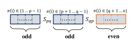
We first determine the positions of and , which are at the -th and -th positions on the -diagonal, respectively. Therefore, there are odd numbers before , odd numbers after , and even numbers before and after . We previously proved that regardless of being odd or even, there exists a permutation that places them on the positive -diagonal.
Specifically, for the odd parts, construct the permutation according to Eq.(5), and for the even parts, construct the permutation according to Eq.(3). Then combine the two disjoint sub-permutations to form the complete permutation.
Since is symmetric, this -diagonal must be positive. Therefore, the matrix is total support,so it can be doubly stochasticized by two diagonal matrices. Given that is symmetric, these two diagonal matrices .
Under the conditions that satisfy the Marcus mapping theorem( is no-negative and , ), the Marcus mapping must exist. We propose the following Marcus algorithm to compute the results obtained from the Marcus mapping.
Input: Symmetric matrix
Output: Doubly stochastic
Adaptive Local doubly stochastic Structure Learning
In graph-based learning, an important aspect is to find a low-dimensional local manifold representation, as high-dimensional data generally contains low-dimensional manifolds. Therefore, selecting an appropriate similarity graph is a crucial requirement for graph-based learning. A reasonable objective function for graph learning is shown below (Nie, Wang, and Huang 2014).
| (8) | ||||
In the research process, is usually considered the probability that and belong to the same class. However, the solution to this problem is not a doubly stochastic matrix, which cannot reasonably express the concept of probability. Therefore, we impose a stronger constraint on problem (LABEL:eq8)
| (9) | ||||
Typically, the learned probability matrix does not have connected components, requiring further clustering using methods like K-means. Due to the following theorem, we introduce the Laplacian rank constraint.
Theorem 3.
For a matrix , if the rank of the Laplacian matrix , then has exactly connected components.
Hence, the Laplacian rank constraint is introduced in, and the final form of the loss function becomes:
| (10) | ||||
Problem (LABEL:eq10) is our objective function. We have designed an optimization algorithm to solve this problem.
Optimization Algorithm
Optimizing problem (LABEL:eq10) is more challenging because the matrix constraints are coupled. However, we can cleverly solve this problem by iteratively solving the relaxed problem and using the Marcus mapping.
Clustering
Assume represents the i-th smallest eigenvalue of . Since is a positive semidefinite matrix, . Because solving for the constraint is too difficult, we relax it to , which means . According to Ky Fan’s Theorem (ky Fan et al.1949), we have
| (11) |
Then problem (10) is equivalent to the following problem
| (12) | ||||
We selected a sufficiently large , so that in the optimization process, can be obtained, thereby solving the relaxed constraint.
Fix , update
Once is fixed, updating only requires solving the following problem
| (13) |
The optimal solution for is the eigenvectors corresponding to the smallest c eigenvalues of . This is part of Ky Fan’s theorem.
Fix , update
Due to the following important equation
| (14) |
we are essentially required to solve the following problem:
| (15) | ||||
Solving this problem is very challenging. Our key idea is to first solve the relaxed problem and then map it to a symmetric doubly stochastic matrix using the Marcus mapping.In this section, we first consider the relaxed problem (15).
| (16) | ||||
Denote and ,Because we relaxed the constraints and decoupled the relationships between rows and columns, we can solve each row independently,Expanding the original problem and simplifying, we ultimately reduce it to the following form, which has a closed-form solution.
| (17) |
By solving this problem, we obtain the optimal solution after relaxation. We transform it into a symmetric matrix using the following symmetrization to meet the conditions for the Marcus mapping.
| (18) |
We will later prove two things: 1. Prove that it is easy to satisfy the conditions of the Marcus mapping by choosing . 2. Prove that the solution obtained through Marcus mapping is sufficiently close to the true solution of problem (LABEL:eq15).
Fix , update
At this step, we utilize the Marcus mapping to compute . Specifically, we input into the Marcus mapping and aim to obtain
| (19) |
After calculating , we substitute it into the first step and iterate through various steps until convergence. We summarize our optimization algorithm in Algorithm 2.
Input: Data matrix , clusters
Parameter: and
Output: Desired similarity graph with connected components
Select based on sparsity
In this part, we will demonstrate how the selection of affects the sparsity of the probability matrix . Additionally, we will prove that by simply choosing we can satisfy the conditions required by the Marcus mapping.
We still consider the relaxed problemLABEL:Eq16 first because if the relaxation problem’s can control the sparsity of the matrix , the non-relaxed one can too. Since we update each row individually, (Nie et al.2016) has proven that the closed-form solution has the following form.
| (20) |
where (Nie, Wang, and Huang 2014). That have k neighbours and . Here, we assume is sorted in descending order with respect to . According to (20) and the value of , we have
| (21) |
where are also sorted in descending order with respect to . This means that by controlling for each row, we can precisely control the sparsity of each row.
Now we demonstrate that we can easily satisfy the conditions required by the Marcus mapping by selecting .
First, we choose , meaning each row has at least two or more elements that are not zero,which means
| (22) |
By choosing , we can ensure that each row of has at least two or more elements that are not zero. Since each element of is greater than zero, also has at least two or more elements that are not zero in each row.
Next, we perform simultaneous row and column exchanges on the symmetric matrix (a congruence transformation of the matrix), ensuring that the superdiagonal and second superdiagonal elements are not zero. Note that this only changes the order of the samples and does not affect the clustering results. Through row and column exchanges, we can satisfy the conditions required by the Marcus mapping.
Approximation Analysis
In this section, we will demonstrate that is sufficiently close to the true solution of problem (LABEL:eq15).
For problem (LABEL:eq8), due to the Karush-Kuhn-Tucker (KKT) conditions, there exist and such that:
| (23) |
where , and , Similarly, considering the transpose problem of problem (LABEL:eq8), we have:
| (24) |
We know that
| (25) | ||||
If are the optimal solutions to problem (LABEL:eq8) and the transpose problem, respectively, then according to Eq. (23) and Eq. (24), is the optimal solution to problem (LABEL:eq9). However, this is usually not the case. Nevertheless, we can have the following estimation:
| (26) | ||||
Usually, is very small relative to , making it an acceptable approximation.
Time Complexity Analysis
Time complexity comparison.
Indeed, in some cases, defining the degree matrix as . and continuously performing the following operations(Ron Zass et al.2005)
| (27) |
can also transform into a doubly stochastic matrix. However, through this method, we need to perform additions, square roots, divisions, and multiplications each round, far exceeding the additions, multiplications and divisions of the Marcus mapping.
If we only consider multiplication, the Marcus mapping takes about half the time compared to the above method.
Time complexity analysis.
When updating by Eq. (13), c smallest eigenvalues need to be computed, Using the Lanczos algorithm can achieve a time complexity that is linear with respect to . Then, the corresponding eigenvectors need to be computed, resulting in a time complexity of , represents the number of iterations.
When updating by the Eq. (17), only n linear equations need to be solve and a matrix addition needs to be calculated, resulting in a time complexity of . Then we calculate Marcus mapping by Algorithm 1, which only requires computing the multiplication of a matrix by a vector and the division of a scalar by a vector, resulting in a time complexity of . Here, represents the number of iterations.
Therefore, the overall time complexity is , represents the total number of iterations.
Connection with Optimal Transport
In this section, we will point out the connection between the Marcus mapping and optimal transport.
Donate the Marcus mapping for a non-negative matrix as , represents the natural logarithm of each element of , and we require and .
Consider the optimal transport problem with entropy regularization:
| (28) | ||||
where
The Lagrangian function of the optimal transport problem is given by
| (29) | ||||
By taking the partial derivative with respect to , we can obtain that the optimal solution satisfies:
| (30) |
In particular, when is 1, the form of the optimal transport solution is consistent with the Marcus mapping.
| (31) |
Since is symmetric,because
| (32) |
is also symmetric, so has the form . This demonstrates that the Marcus mapping is solving a special optimal transport.
The transformation of is crucial as it can convert zeros in the probability matrix to positive values, thereby satisfying the conditions for optimal transport. However, computing through the Marcus mapping is much more efficient than directly using optimal transport, primarily because optimal transport involves additional logarithmic computations, and expressing in a computer is challenging.
Experiments on toy datasets
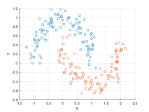
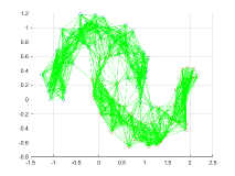
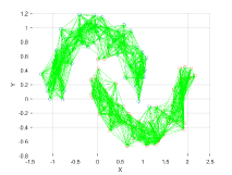
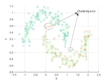
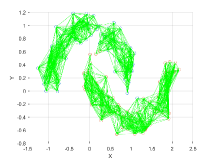
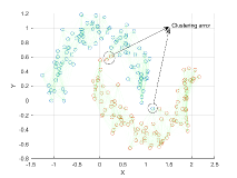
To demonstrate the superiority of our algorithm, we first constructed a toy dataset in the shape of double moons. We set the sample size to 200, with a random seed of 1 and noise level of 0.13. We performed clustering using both the CAN and ANCMM algorithms, both of which incorporate rank constraints and are adaptive neighbors algorithms. We compared their accuracy and the configuration of adaptive neighbors. The dataset and results are shown in Figure 2.
| Metric | CAN | ADCMM | Metric | CAN | ADCMM | Metric | CAN | ADCMM |
| ACC | 98.0 | 98.5 | NMI | 86.2 | 88.9 | PUR | 98.0 | 98.5 |
We used the learned probability matrix weights as the edge weights connecting each pair of points.Additionally, we demonstrate the similarity matrix obtained solely from the Gaussian kernel function. Both CAN(Nie.et 2010) and ANCMM learned similarity matrix with two connected components. However, as shown in the figure, CAN misclassified one more point compared to ANCMM. Table 1 shows the accuracy(ACC), normalized mutual information(NMI), and purity (PUR) metrics for the clustering results.
Experiments on real datasets
Experimental Settings
Datasets.
We conducted extensive experiments on ten datasets, including TR41,ORL,ARsmall,LetterRecognition,
warpPIE10P,Wine,Feret,Movement,Ecoil,Yeast. The Table 2 lists the number of samples and clusters for each dataset:
| Datasets | Object | Attribute | Class |
|---|---|---|---|
| TR41 | 878 | 7454 | 10 |
| ORL | 400 | 1024 | 40 |
| ARsmall | 2600 | 1260 | 100 |
| LetterRecognition | 780 | 16 | 26 |
| Yale | 165 | 256 | 15 |
| Wine | 178 | 13 | 3 |
| Feret | 1400 | 1024 | 4 |
| Movement | 360 | 90 | 15 |
| Ecoil | 336 | 7 | 8 |
| Yeast | 165 | 1024 | 15 |
Compared Methods.
To demonstrate the superiority of our algorithm ANCMM, we compare it with various state-of-the-art algorithms.We chose the K-Means algorithm, Spectral Clustering(SC) algorithm, CAN algorithm(Nie et al. 2014), and DSDC algorithm(He et al. 2023) for comparison. Among them, the CAN algorithms is adaptive neighbor algorithms, and the DSDC algorithm is a symmetric doubly stochastic algorithm. When using each algorithm, we applied the same preprocessing to the data to ensure fairness.
| Method | K-Means | SC | DSDC | CAN | ERCAN | OUR |
|---|---|---|---|---|---|---|
| TR41 | 63.7 | 72.1 | 66.0 | 71.8 | 75.1 | 73.1 |
| ORL | 56.3 | 53.5 | 60.5 | 58.0 | 57.0 | 61.5 |
| ARsmall | 13.38 | 14.3 | 13.38 | 14.6 | 18.3 | 15.81 |
| LetterRecognition | 32.7 | 33.9 | 34.7 | 32.1 | 31.0 | 35.0 |
| Yale | 45.5 | 47.9 | 50.3 | 52.1 | 47.9 | 52.1 |
| Wine | 97.2 | 97.2 | 89.9 | 97.2 | 47.8 | 98.3 |
| Feret | 29.6 | 25.9 | 29.7 | 29.7 | 25.6 | 31.0 |
| Movement | 47.0 | 50.8 | 41.4 | 50.2 | 47.8 | 50.6 |
| Ecoil | 80.4 | 56.6 | 54.2 | 83.6 | 57.4 | 83.9 |
| Yeast | 48.7 | 42.0 | 34.0 | 48.9 | 43.3 | 50.1 |
| Method | K-Means | SC | DSDC | CAN | ERCAN | OUR |
|---|---|---|---|---|---|---|
| TR41 | 67.3 | 70.9 | 67.4 | 72.3 | 75.6 | 74.7 |
| ORL | 74.8 | 73.2 | 76.7 | 73.5 | 74.9 | 75.7 |
| ARsmall | 42.3 | 42.8 | 40.9 | 37.0 | 37.3 | 38.6 |
| LetterRecognition | 44.3 | 45.4 | 46.7 | 39.8 | 40.5 | 42.3 |
| Yale | 52.9 | 51.4 | 53.9 | 60.5 | 54.3 | 59.2 |
| Wine | 89.0 | 89.0 | 73.2 | 89.0 | 83.0 | 92.6 |
| Feret | 67.2 | 63.0 | 63.0 | 61.3 | 62.2 | 64.3 |
| Movement | 59.0 | 60.9 | 52.8 | 63.5 | 62.4 | 64.0 |
| Ecoil | 66.0 | 53.9 | 51.2 | 71.3 | 51.9 | 73.6 |
| Yeast | 28.0 | 27.7 | 23.0 | 29.6 | 47.9 | 29.8 |
| Method | K-Means | SC | DSDC | CAN | ERCAN | OUR |
|---|---|---|---|---|---|---|
| TR41 | 83.5 | 85.3 | 85.1 | 84.7 | 85.8 | 85.9 |
| ORL | 61.3 | 59.0 | 63.0 | 63.8 | 59.3 | 64.8 |
| ARsmall | 13.8 | 14.6 | 13.9 | 16.0 | 19.1 | 16.7 |
| LetterRecognition | 34.9 | 35.3 | 36.5 | 35.6 | 33.7 | 38.9 |
| Yale | 48.5 | 48.5 | 51.5 | 52.7 | 50.3 | 52.7 |
| Wine | 97.2 | 97.2 | 89.9 | 97.2 | 94.9 | 98.3 |
| Feret | 32.6 | 28.6 | 32.0 | 34.6 | 29.2 | 34.3 |
| Movement | 50.0 | 51.7 | 46.1 | 51.9 | 51.1 | 51.7 |
| Ecoil | 82.7 | 83.9 | 82.1 | 84.8 | 81.9 | 85.7 |
| Yeast | 55.3 | 55.3 | 52.5 | 50.7 | 45.8 | 51.0 |
Parameters Selection.
Our model has two parameters, and . is adaptive in the experiments, we randomly select a positive . If in each iteration is greater than , we set , otherwise, we set , until final convergence.As for , we ran only once with the initialization described in Eq. (22).For the other methods, we randomly initialize and take the best result after 30 runs.
Evaluation Metrics.
In the experiments, we used accuracy (ACC), normalized mutual information (NMI), and purity (PUR) to evaluate the results. Tables 3, 4 and 5 present the corresponding results.
Experimental Result
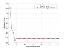
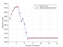
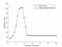
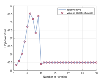
To illustrate the convergence of our algorithm, we selected four datasets: Ecoli, Wine, Movement, and LetterRecognition. We plotted their convergence curves, as shown in Figure 3. According to the results, our algorithm typically converges in around 10 iterations
Conclusions
This paper proves the theorems related to the Marcus mapping and proposes a clustering method based on Marcus mapping, called Doubly Stochastic Adaptive Neighbors Clustering (ANCMM). Under rank constraint conditions, the similarity matrix obtained can be directly partitioned into specific clusters, and the similarity matrix is doubly stochastic and symmetric. We also discuss the relationship between Marcus mapping and optimal transport, illustrating that Marcus mapping solves a special form of optimal transport, but the computation through Marcus mapping is superior to that through optimal transport. Future work can explore the application of Marcus mapping and rank constraints in other fields such as dimension reduction.
References
- Bai and Liang (2020) Bai, L.; and Liang, J. 2020. Sparse subspace clustering with entropy-norm. In International conference on machine learning, 561–568. PMLR.
- Barrio-Hernandez et al. (2023) Barrio-Hernandez, I.; Yeo, J.; Jänes, J.; Mirdita, M.; Gilchrist, C. L.; Wein, T.; Varadi, M.; Velankar, S.; Beltrao, P.; and Steinegger, M. 2023. Clustering predicted structures at the scale of the known protein universe. Nature, 622(7983): 637–645.
- Cuturi (2013) Cuturi, M. 2013. Sinkhorn distances: Lightspeed computation of optimal transport. Advances in neural information processing systems, 26.
- Ding et al. (2022) Ding, T.; Lim, D.; Vidal, R.; and Haeffele, B. D. 2022. Understanding Doubly Stochastic Clustering. In Proceedings of the 39th International Conference on Machine Learning, volume 162 of Proceedings of Machine Learning Research, 5153–5165. PMLR.
- Huang et al. (2023) Huang, W.; Chen, C.; Li, Y.; Li, J.; Li, C.; Song, F.; Yan, Y.; and Xiong, Z. 2023. Style projected clustering for domain generalized semantic segmentation. In Proceedings of the IEEE/CVF conference on computer vision and pattern recognition, 3061–3071.
- Ju et al. (2023) Ju, W.; Gu, Y.; Chen, B.; Sun, G.; Qin, Y.; Liu, X.; Luo, X.; and Zhang, M. 2023. Glcc: A general framework for graph-level clustering. In Proceedings of the AAAI conference on artificial intelligence, volume 37, 4391–4399.
- Marcus and Newman (1961) Marcus, M.; and Newman, M. 1961. The permanent of a symmetric matrix. Notices Amer. Math. Soc, 8: 595.
- Meng et al. (2023) Meng, Z.; Zhao, P.; Yu, Y.; and King, I. 2023. Doubly stochastic graph-based non-autoregressive reaction prediction. arXiv preprint arXiv:2306.06119.
- Nie et al. (2017) Nie, F.; Li, J.; Li, X.; et al. 2017. Self-weighted multiview clustering with multiple graphs. In IJCAI, 2564–2570.
- Nie, Wang, and Huang (2014) Nie, F.; Wang, X.; and Huang, H. 2014. Clustering and projected clustering with adaptive neighbors. In Proceedings of the 20th ACM SIGKDD international conference on Knowledge discovery and data mining, 977–986.
- Nie et al. (2016) Nie, F.; Wang, X.; Jordan, M.; and Huang, H. 2016. The constrained laplacian rank algorithm for graph-based clustering. In Proceedings of the AAAI conference on artificial intelligence, volume 30.
- Nie et al. (2011) Nie, F.; Zeng, Z.; Tsang, I. W.; Xu, D.; and Zhang, C. 2011. Spectral Embedded Clustering: A Framework for In-Sample and Out-of-Sample Spectral Clustering. IEEE Transactions on Neural Networks, 22(11): 1796–1808.
- Peyré, Cuturi et al. (2019) Peyré, G.; Cuturi, M.; et al. 2019. Computational optimal transport: With applications to data science. Foundations and Trends® in Machine Learning, 11(5-6): 355–607.
- Sander et al. (2022) Sander, M. E.; Ablin, P.; Blondel, M.; and Peyré, G. 2022. Sinkformers: Transformers with doubly stochastic attention. In International Conference on Artificial Intelligence and Statistics, 3515–3530. PMLR.
- Sinkhorn and Knopp (1967) Sinkhorn, R.; and Knopp, P. 1967. Concerning nonnegative matrices and doubly stochastic matrices. Pacific Journal of Mathematics, 21(2): 343–348.
- Van Assel et al. (2024) Van Assel, H.; Vayer, T.; Flamary, R.; and Courty, N. 2024. Snekhorn: Dimension reduction with symmetric entropic affinities. Advances in Neural Information Processing Systems, 36.
- Villani (2003) Villani, C. 2003. Topics in Optimal Transportation. 58. American Mathematical Soc.
- Wang et al. (2022) Wang, J.; Ma, Z.; Nie, F.; and Li, X. 2022. Entropy regularization for unsupervised clustering with adaptive neighbors. Pattern Recognition, 125: 108517.
- Yan et al. (2024) Yan, Y.; Xu, Z.; Yang, C.; Zhang, J.; Cai, R.; and Ng, M. K.-P. 2024. An Optimal Transport View for Subspace Clustering and Spectral Clustering. In Proceedings of the AAAI Conference on Artificial Intelligence, volume 38, 16281–16289.
- Zass and Shashua (2005) Zass, R.; and Shashua, A. 2005. A unifying approach to hard and probabilistic clustering. In Tenth IEEE International Conference on Computer Vision (ICCV’05) Volume 1, volume 1, 294–301. IEEE.
- Zass and Shashua (2006) Zass, R.; and Shashua, A. 2006. Doubly stochastic normalization for spectral clustering. Advances in neural information processing systems, 19.
- Zong et al. (2024) Zong, L.; Miao, F.; Zhang, X.; Liang, W.; and Xu, B. 2024. Self-Supervised Deep Multiview Spectral Clustering. IEEE Transactions on Neural Networks and Learning Systems, 35(3): 4299–4308.