STATUS: arXiv pre-print

On the construction of scattering matrices for irregular
or elongated enclosures using Green’s representation formula

Carlos Borges 
University of Central Florida, Department of Mathematics
Orlanda, FL 32816

carlos.borges@ucf.edu

Leslie Greengard 
Center for Computational Mathematics
Flatiron Institute
New York, NY 10010 and
Courant Institute, New York University
New York, NY 10012
lgreengard@flatironinstitute.org

Michael O’Neil 
Center for Computational Mathematics
Flatiron Institute
New York, NY 10010
moneil@flatironinstitute.org

Manas Rachh 
Center for Computational Mathematics
Flatiron Institute
New York, NY 10010
mrachh@flatironinstitute.org

Abstract

Multiple scattering methods are widely used to reduce the computational complexity of acoustic or electromagnetic scattering problems when waves propagate through media containing many identical inclusions. Historically, this numerical technique has been limited to situations in which the inclusions (particles) can be covered by nonoverlapping disks in two dimensions or spheres in three dimensions. This allows for the use of separation of variables in cylindrical or spherical coordinates to represent the solution to the governing partial differential equation. Here, we provide a more flexible approach, applicable to a much larger class of geometries. We use a Green’s representation formula and the associated layer potentials to construct incoming and outgoing solutions on rectangular enclosures. The performance and flexibility of the resulting scattering operator formulation in two-dimensions is demonstrated via several numerical examples for multi-particle scattering in free space as well as in layered media. The mathematical formalism extends directly to the three dimensional case as well, and can easily be coupled with several commercial numerical PDE software packages.

Keywords— Helmholtz equation, multiple particle scattering, scattering matrix, irregular or elongated enclosures

1 Introduction

A powerful tool in the analysis of wave propagation problems in domains with many inclusions is multiple scattering theory (see, for example, [6, 24, 26, 29, 32, 36, 34, 48] and the monographs [5, 41, 28, 42]). The workhorse in this approach is the construction of the scattering operator or matrix for an irregular compact inclusion – typically obtained from computing the map from incoming data to outgoing scattered solutions on an enclosing disk (circle) in the plane or an enclosing ball (sphere) in three dimensions. We will refer to the enclosing surfaces as proxy surfaces. For simplicity, here we restrict our attention to the two-dimensional acoustic scattering case (extensions to three dimensions and other elliptic PDEs are relatively straightforward), where the governing equation is the scalar Helmholtz equation

$$\Delta u+k^{2}u=0,$$ (1.1)

with $k$ a complex wavenumber with non-negative imaginary part. Given a disk $D$ of radius $R$, solutions of (1.1) that are regular inside the disk can be represented as

$$\sum_{n=-\infty}^{\infty}\alpha_{n}\,J_{n}(kr)\,e^{in\theta},$$ (1.2)

where $(r,\theta)$ are the polar coordinates of a point with respect to the disk center and $J_{n}$ denotes the $n$th-order Bessel function of the first kind. Solutions of (1.1) that are regular outside the disk and which satisfy the Sommerfeld radiation condition

$$\lim_{r\rightarrow\infty}r^{1/2}\left(\frac{\partial u}{\partial r}-iku\right)=0$$ (1.3)

can be represented as

$$\sum_{n=-\infty}^{\infty}\beta_{n}\,H_{n}(kr)\,e^{in\theta},$$ (1.4)

where $H_{n}$ is the $n$th-order Hankel function of the first kind. In this basis of Bessel functions, given an incoming field sampled on the boundary of the disk as a finite Fourier series, the scattering operator maps the vector of Fourier coefficients $\{\alpha_{n}\}$ to the corresponding coefficients $\{\beta_{n}\}$ of the truncated outgoing expansion (1.4). The construction of the scattering operator, of course, requires the one-time solution of a collection of boundary value problems on the inclusion itself, the details of which depend on the material properties of the inclusion.

This classical theory is simple because the expansions (1.2) and (1.4) are explicit bases for solutions of the Helmholtz equation (obtained by separation of variables). In practice, however, this approach fails when the inclusions are moderately close to touching and far from circular in shape (see Fig. 1) due to the slow convergence or divergence of such expansions.

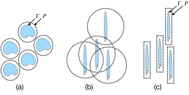
Figure 1: In multiple scattering methods, each inclusion with boundary $\Gamma$ is enclosed in a proxy surface $P$. For any incoming field, sampled on $P$, the scattering matrix yields a representation for the outgoing field induced on $\Gamma$ (but only in the exterior of $P$). These methods work well when inclusions are spatially separated. When $P$ is a disk, as in (a), even fairly close interactions can be accurately computed, requiring only that the enclosing disks are disjoint. For high aspect ratio inclusions, as in (b), they fail since the enclosing disks overlap even when there is a significant gap between them. Here, we extend the approach by constructing scattering matrices on more closely contoured enclosures such as a rectangle, as depicted in (c).

In this paper, we describe a new technique for acoustic or electromagnetic scattering from complex microstructured materials in two dimensions, governed by (1.1), assuming only that the inclusions are identical up to rotation and translation (or drawn from a small set of such particles). The power of the approach, as with classical multiple scattering methods, is that it yields efficient algorithms for microstructure design – in the context of an outer optimization process, each new configuration requires the calculation of an objective function which, in general, depends on the scattered field. With thousands of inclusions, this is intractable when done directly. The use of scattering matrices can dramatically reduce the number of degrees of freedom in such calculations as well as the condition number of the full problem so that such design loops become computationally feasible, especially when coupled with fast algorithms to compute the interactions between the individual inclusions.

We summarize the necessary background from potential theory in the next section, followed by a description of the construction of generalized scattering operators. We then apply the method to rectangular enclosures and demonstrate its performance in both free space and layered media. We will use the terms enclosure and proxy surface interchangeably. It is worth noting that the solver used for modeling individual inclusions when constructing the scattering matrix can be called in “black box” fashion, and easily coupled to any commercial or non-commercial software packages.

Remark 1.

There is an alternative to defining scattering matrices on enclosures that has emerged over the last decade or so. Namely, modern fast direct solvers can (a) sample the incoming field on the obstacle itself, and (b) solve an associated integral equation to obtain an equivalent charge or dipole distribution along the surface of the obstacle (or an enclosing proxy surface) that accurately reproduces the scattered solution in the far field. This representation can be compressed by identifying a subset of points on the surface that are sufficient to represent both the incoming and scattered fields. The map from the incoming field sampled at those points to the charge/dipole strengths induced at those points is itself a kind of scattering matrix. This idea was used in a principled hierarchical manner to construct fast direct solvers for non-oscillatory elliptic integral equations on planar domains with corners in [7] and on smooth surfaces in three dimensions in [9]. We will refer to this approach as skeletonization. In some applications it may be beneficial to construct scattering matrices through skeletonization, while in others it may be more practical to build a few “standard” scattering matrices in the sense depicted in Fig. 1. We will return to this question in the concluding section.

2 Mathematical preliminaries

In this section, we summarize the properties of layer potentials using the Green’s function for the scalar Helmholtz equation (1.1), given by

$$g_{k}(\boldsymbol{x},\boldsymbol{y})=\frac{i}{4}H_{0}^{(1)}(k|\boldsymbol{x}-\boldsymbol{y}|)\,,$$ (2.1)

where $H_{0}^{(1)}$ is the zeroth-order Hankel function of the first kind. The variables $\boldsymbol{x}=(x_{1},x_{2})$ and $\boldsymbol{y}=(y_{1},y_{2})$ denote points in $\mathbb{R}^{2}$. See [16] for a thorough discussion of this Green’s function.

2.1 Layer potentials

Given a closed curve $\Gamma$ and densities $\sigma$ and $\mu$ supported along this curve, we define the standard single and double layer potentials $\mathcal{S}_{\Gamma}[\sigma]$ and $\mathcal{D}_{\Gamma}[\mu]$ by

$$\mathcal{S}_{\Gamma}[\sigma](\boldsymbol{x}) =\int_{\Gamma}g_{k}(\boldsymbol{x},\boldsymbol{y})\,\sigma(\boldsymbol{y})\,ds,$$ (2.2)

$$\mathcal{D}_{\Gamma}[\mu](\boldsymbol{x}) =\int_{\Gamma}\left(\boldsymbol{n}(\boldsymbol{y})\cdot\nabla_{\boldsymbol{y}}g_{k}(\boldsymbol{x},\boldsymbol{y})\right)\mu(\boldsymbol{y})\,ds,$$

where it is assumed that $\boldsymbol{x}\notin\Gamma$. These potentials automatically satisfy the Sommerfeld radiation condition (1.3), and furthermore, for $\boldsymbol{x}\notin\Gamma$ they are infinitely differentiable functions. For values of $\boldsymbol{x}$ on the boundary $\Gamma$, the potentials are well-defined in terms of weakly singular integral operators, denoted by $S_{\Gamma}$ and $D_{\Gamma}$. For $\boldsymbol{x}_{0}\in\Gamma$, these satisfy the jump relations

$$\lim_{\begin{subarray}{c}\boldsymbol{x}\to\boldsymbol{x}_{0}\\ \boldsymbol{x}\in\Omega^{\pm}\end{subarray}}\mathcal{S}_{\Gamma}[\sigma](\boldsymbol{x}) =\mathrm{S}_{\Gamma}[\sigma](\boldsymbol{x}_{0})\,,$$ (2.3)

$$\lim_{\begin{subarray}{c}\boldsymbol{x}\to\boldsymbol{x}_{0}\\ \boldsymbol{x}\in\Omega^{\pm}\end{subarray}}\mathcal{D}_{\Gamma}[\mu](\boldsymbol{x}) =\pm\frac{\mu(\boldsymbol{x}_{0})}{2}+\mathrm{D}_{\Gamma}[\mu](\boldsymbol{x}_{0})\,.$$

Next, consider an enclosure or proxy surface $P$ with $\Gamma$ in its interior, as shown earlier in Fig. 1. Let the unit outward normal along $P$ be denoted by $\boldsymbol{n}$. The normal derivatives of $\mathcal{S}_{\Gamma}[\sigma]$ and $\mathcal{D}_{\Gamma}[\mu]$ along $P$ are defined as:

$$\mathcal{S}^{\prime}_{\Gamma\rightarrow P}[\sigma](\boldsymbol{x}) =\boldsymbol{n}(\boldsymbol{x})\cdot\nabla\mathcal{S}_{\Gamma}[\sigma](\boldsymbol{x}),$$ (2.4)

$$\mathcal{D}^{\prime}_{\Gamma\rightarrow P}[\mu](\boldsymbol{x}) =\boldsymbol{n}(\boldsymbol{x})\cdot\nabla_{\boldsymbol{x}}\mathcal{D}_{\Gamma}[\mu](\boldsymbol{x}).$$

In general, given two disjoint oriented curves $\Gamma_{1}$ and $\Gamma_{2}$, we will denote by $\mathcal{S}_{\Gamma_{1}\rightarrow\Gamma_{2}}[\sigma]$ the restriction of the layer potential $\mathcal{S}_{\Gamma_{1}}[\sigma]$ to points $\boldsymbol{x}\in\Gamma_{2}$. (The same notation will be used for $\mathcal{D}$.) In a slight abuse of notation, when $\Gamma_{2}=\Gamma_{1}=\Gamma$, we will refer to the weakly singular operators $S_{\Gamma\rightarrow\Gamma}$ and $D_{\Gamma\rightarrow\Gamma}$ as $S_{\Gamma}$, $D_{\Gamma}$ (as was done above). Finally, we will denote a function $u:\mathbb{R}^{2}\to\mathbb{C}$ restricted to a closed curve $P$ by $u|_{P}$.

2.2 Combined field integral equation

While the scattering operator construction described below is independent of the material properties of the inclusion, for the sake of concreteness, we assume that, using the language of acoustics, it is sound-soft [16]. That is, given an incoming (pressure) field $u^{\textrm{in}}$, the total pressure $u=u^{\textrm{in}}+u^{\textrm{sc}}$ must satisfy the homogeneous Dirichlet condition $u=0$ so that $u^{\textrm{sc}}=-u^{\textrm{in}}$ on the inclusion boundary $\Gamma$. The classical integral equation for such problems makes use of the combined field representation

$$u^{\textrm{sc}}(\boldsymbol{x})=\mathcal{D}_{\Gamma}[\sigma](\boldsymbol{x})+ik\mathcal{S}_{\Gamma}[\sigma](\boldsymbol{x})\,,\quad\boldsymbol{x}\in\Omega^{c}\,.$$ (2.5)

Using the jump relations in 2.3, $\sigma$ can be shown to be given by [16]

$$\sigma=-\left(\frac{1}{2}+\mathrm{D}_{\Gamma}+ik\mathrm{S}_{\Gamma}\right)^{-1}u^{\textrm{in}}|_{\Gamma}\,.$$ (2.6)

2.3 Green’s identities

Suppose that a function $u$ satisfies the Helmholtz equation in the interior $\Omega$ of a closed curve $\Gamma$. Green’s representation formula [16] states that for any $\boldsymbol{x}\in\Omega$,

$$u(\boldsymbol{x})=-\mathcal{D}_{\Gamma}[u](\boldsymbol{x})+\mathcal{S}_{\Gamma}\left[\frac{\partial u}{\partial n}\right](\boldsymbol{x})$$ (2.7)

where $\partial/\partial n$ denotes the directional derivative in the direction of $\boldsymbol{n}$, the unit outward normal to $\Gamma$ (i.e. the direction pointing into the unbounded domain $\Omega^{c}$). Furthermore, assuming a function $v$ satisfies the Helmholtz equation in the region $\Omega^{c}$ exterior to $\Omega$, we have

$$v(\boldsymbol{x})=\mathcal{D}_{\Gamma}[v](\boldsymbol{x})-\mathcal{S}_{\Gamma}\left[\frac{\partial v}{\partial n}\right](\boldsymbol{x}).$$ (2.8)

The flip in signs is due to the definition of the normal direction $\boldsymbol{n}$.

3 Scattering operator construction

We now turn to describing a method for constructing a scattering operator using nothing more than the Green’s representation identities given in the previous section.

Let $P$ be a rectangle that encloses a sound-soft obstacle $\Omega$ with boundary $\Gamma$, and let $\Omega_{P}$ denote the interior of $P$. The scattering operator in this formulation is a map from values of the incoming data $(u^{\textrm{in}},\frac{\partial u}{\partial n}^{\textrm{in}})$ on $P$ to samples of the scattered field $(u^{\textrm{sc}},\frac{\partial u}{\partial n}^{\textrm{sc}})$ on $P$. Since $u^{\textrm{in}}$ is assumed to satisfy the homogeneous Helmholtz equation inside $P$, we may use Green’s representation formula (2.7) to obtain

$$u^{\textrm{in}}(\boldsymbol{x})=-\mathcal{D}_{P}\left[u^{\textrm{in}}\right](\boldsymbol{x})+\mathcal{S}_{P}\left[\frac{\partial u}{\partial n}^{\textrm{in}}\right](\boldsymbol{x})\,,\quad\boldsymbol{x}\in\Omega_{P}\,.$$ (3.1)

This is a parameterization of $u^{\textrm{in}}$ in terms of its boundary data along $P$. Given $u^{\textrm{in}}$ along $\Gamma$, we can solve (2.6) to obtain the density $\sigma$ along $\Gamma$ and then evaluate the scattered field for $\boldsymbol{x}\in P$ as

$$u^{\textrm{sc}}(\boldsymbol{x}) =\mathcal{D}_{\Gamma\rightarrow P}[\sigma](\boldsymbol{x})+ik\mathcal{S}_{\Gamma\rightarrow P}[\sigma](\boldsymbol{x})\,,$$ (3.2)

$$\frac{\partial u}{\partial n}^{\textrm{sc}}(\boldsymbol{x}) ={\mathcal{D}}^{\prime}_{\Gamma\rightarrow P}[\sigma](\boldsymbol{x})+ik{\mathcal{S}}^{\prime}_{\Gamma\rightarrow P}[\sigma](\boldsymbol{x})\,.$$

Finally, combining equations 3.1, 2.6 and 3.2, the scattering operator which maps the incoming data and its normal derivative to the scattered field and its normal derivative, which we will denote by $\mathrm{A}^{\Gamma}_{P}$, is given by the following composition of operators:

$$\mathrm{A}^{\Gamma}_{P}=\begin{bmatrix}{\mathcal{D}}_{\Gamma\rightarrow P}+ik{\mathcal{S}}_{\Gamma\rightarrow P}\\ {\mathcal{D}}^{\prime}_{\Gamma\rightarrow P}+ik{\mathcal{S}}^{\prime}_{\Gamma\rightarrow P}\end{bmatrix}\left(\frac{1}{2}+\mathrm{D}_{\Gamma}+ik\mathrm{S}_{\Gamma}\right)^{-1}\begin{bmatrix}{\mathcal{D}}_{P\rightarrow\Gamma}&-{\mathcal{S}}_{P\rightarrow\Gamma}\end{bmatrix}\,.$$ (3.3)

That is to say,

$$\begin{bmatrix}u^{\textrm{sc}}|_{P}\\ \frac{\partial u}{\partial n}^{\textrm{sc}}|_{P}\end{bmatrix}=\mathrm{A}^{\Gamma}_{P}\begin{bmatrix}u^{\textrm{in}}|_{P}\\ \frac{\partial u}{\partial n}^{\textrm{in}}|_{P}\end{bmatrix}\,.$$ (3.4)

Lastly, suppose that $\Gamma$ and $\Gamma^{\prime}$ are related by a unitary affine transformation, and that the corresponding proxy surfaces $P$ and $P^{\prime}$ are related by the same unitary affine transformation. Then, due to the translation and rotation invariance of the Helmholtz operator, the associated scattering operators are identical, i.e. $\mathrm{A}^{\Gamma}_{P}=\mathrm{A}^{\Gamma^{\prime}}_{P^{\prime}}$.

3.1 Multi-particle scattering

We now consider the classical problem of scattering from a collection of $M$ obstacles $\Omega_{j}$ with boundaries given by $\Gamma_{j}=\partial\Omega_{j}$, for $j=1,\dots,M$. As above, let $P_{j}$ denote a rectangle enclosing $\Gamma_{j}$ and let $\Omega_{P_{j}}$ denote its interior. In general, and in what follows, there is no assumption that the obstacles are identical or related by affine transformations. If this happens to be the case, then each $P_{j}$ can be constructed from an affine transformation of a canonical $P$, and the resulting scattering operators will be identical.

We may represent the total field in the exterior of all proxy surfaces by

$$u=\sum_{j=1}^{M}\left(\mathcal{D}_{P_{j}}\left[u^{\textrm{sc}}\right]-\mathcal{S}_{P_{j}}\left[\frac{\partial u}{\partial n}^{\textrm{sc}}\right]\right)+u^{\textrm{in}}\,,$$ (3.5)

using Green’s representation theorem. Since the scattering operator accounts for the response of each inclusion to an arbitrary incoming field, the condition that needs to be satisfied is simply the continuity of the potential and its normal derivative on the (artificial) proxy surfaces boundaries. That is, on enclosure $P_{i}$, we must have

$$\begin{bmatrix}u^{\textrm{sc}}|_{P_{i}}\\ \frac{\partial u}{\partial n}^{\textrm{sc}}|_{P_{i}}\end{bmatrix}-\sum_{\begin{subarray}{c}j=1\\ j\neq i\end{subarray}}^{M}\begin{bmatrix}{\mathcal{D}}_{P_{j}\rightarrow P_{i}}&-{\mathcal{S}}_{P_{j}\rightarrow P_{i}}\\ {\mathcal{D}}^{\prime}_{P_{j}\rightarrow P_{i}}&-{\mathcal{S}}^{\prime}_{P_{j}\rightarrow P_{i}}\end{bmatrix}\begin{bmatrix}u^{\textrm{sc}}|_{P_{j}}\\ \frac{\partial u}{\partial n}^{\textrm{sc}}|_{P_{j}}\end{bmatrix}\\ =\mathrm{A}^{\Gamma}_{P_{i}}\left(\begin{bmatrix}u^{\textrm{in}}|_{P_{i}}\\ \frac{\partial u}{\partial n}^{\textrm{in}}|_{P_{i}}\end{bmatrix}+\sum_{\begin{subarray}{c}j=1\\ j\neq i\end{subarray}}^{M}\begin{bmatrix}{\mathcal{D}}_{P_{j}\rightarrow P_{i}}&-{\mathcal{S}}_{P_{j}\rightarrow P_{i}}\\ {\mathcal{D}}^{\prime}_{P_{j}\rightarrow P_{i}}&-{\mathcal{S}}^{\prime}_{P_{j}\rightarrow P_{i}}\end{bmatrix}\begin{bmatrix}u^{\textrm{sc}}|_{P_{j}}\\ \frac{\partial u}{\partial n}^{\textrm{sc}}|_{P_{j}}\end{bmatrix}\right)\,.$$ (3.6)

Omitting the algebra, the left-hand side of (3.6) is the contribution of the scattered field from scatterer $\Omega_{i}$ to the net scattered field, as seen from representation (3.5), and the right hand side encodes the response of the $i$th inclusion to the total incoming field. The above equations provide the setup for the classical multiple scattering formalism [41, 24].

Let the operators $\mathcal{A}$, $\mathrm{T}_{ij}$, and $\mathcal{T}$ be given by

$$\mathcal{A}=\begin{bmatrix}\mathrm{A}_{P_{1}}^{\Gamma_{1}}&0&\ldots&0\\ 0&\mathrm{A}_{P_{1}}^{\Gamma_{2}}&\ldots&0\\ \vdots&\vdots&\ddots&\vdots\\ 0&0&\ldots&\mathrm{A}_{P_{M}}^{\Gamma_{M}}\end{bmatrix}\,,$$ (3.7)

$$T_{ij}=\begin{bmatrix}{\mathcal{D}}_{P_{j}\rightarrow P_{i}}&-{\mathcal{S}}_{P_{j}\rightarrow P_{i}}\\ {\mathcal{D}}^{\prime}_{P_{j}\rightarrow P_{i}}&-{\mathcal{S}}^{\prime}_{P_{j}\rightarrow P_{i}}\end{bmatrix}\,.$$ (3.8)

and

$$\mathcal{T}=\begin{bmatrix}0&\mathrm{T}_{12}&\ldots&\mathrm{T}_{1M}\\ \mathrm{T}_{21}&0&\ldots&\mathrm{T}_{2M}\\ \vdots&\vdots&\ddots&\vdots\\ \mathrm{T}_{M1}&\mathrm{T}_{M2}&\ldots&0\end{bmatrix}\,,$$ (3.9)

Using these definitions, the classical multiple scattering system (3.6) can be written concisely in linear algebraic form as:

$$\left(I-(\mathcal{A}+I)\mathcal{T}\right)\begin{bmatrix}u^{\textrm{sc}}|_{P_{1}}\\ \frac{\partial u}{\partial n}^{\textrm{sc}}|_{P_{1}}\\ \vdots\\ u^{\textrm{sc}}|_{P_{M}}\\ \frac{\partial u}{\partial n}^{\textrm{sc}}|_{P_{M}}\end{bmatrix}=\mathcal{A}\begin{bmatrix}u^{\textrm{in}}|_{P_{1}}\\ \frac{\partial u}{\partial n}^{\textrm{in}}|_{P_{1}}\\ \vdots\\ u^{\textrm{in}}|_{P_{M}}\\ \frac{\partial u}{\partial n}^{\textrm{in}}|_{P_{M}}\end{bmatrix}\,.$$ (3.10)

The right hand side above only needs to be computed once, and assuming that the inclusions are not extremely close-to-touching, solving the above system using an iterative solver, such as GMRES, usually only requires a modest number of iterations (particularly when a diagonal preconditioner is used [24]).

4 Multiple scattering in a layered medium

In many applications, including meta-material design [49, 4], a collection of identically-shaped scatterers are embedded in a layered medium to achieve some response of interest (such as focusing an incoming wave). For this, the multiple scattering framework above needs to be modified to include the effect of the layered medium itself. This has been done previously using classical scattering matrices (see, for example, [36, 38]).

We show in this section how to extend our approach in the simplest setting: when a collection of $M$ obstacles with boundaries $\Gamma_{j}$ as well as their enclosures $P_{j}$, $j=1,2,\ldots M$, lie in the upper half plane $\Omega_{+}=\{(x_{1},x_{2})\,|\,x_{2}>0\}$. We denote by $\Omega_{-}=\{(x_{1},x_{2})\,|\,x_{2}<0\}$ the lower half plane and assume that $x_{2}=0$ is an acoustic interface with wavenumbers in the upper and lower half planes given by $k_{\pm}$, respectively. A canonical transmission condition along $x_{2}=0$ is that the total field and its normal derivative are continuous across the interface. We let $u^{\textrm{sc}}_{\pm}$ denote the scattered field in the upper or lower half-space, respectively, and with a slight abuse of notation, will use $u^{\textrm{sc}}$ without the subscript when the context is clear. The extension to layered media is somewhat detailed but straightforward, so long as each inclusion is completely contained in a single layer.

4.1 The layered medium Green’s function

The simplest way to account for the presence of the infinite acoustic interface is through the construction of the layered medium Green’s function $g^{LM}$. In what follows, we will assume that the source $\boldsymbol{y}$ is located in the upper half plane and that the target $\boldsymbol{x}$ can be located anywhere in $\mathbb{R}^{2}$. An analogous definition of $g^{LM}$ can be constructed when the source is in the lower half plane. The layered medium Green’s function is then defined as

$$g^{LM}(\boldsymbol{x},\boldsymbol{y})=\begin{cases}g_{k_{+}}(\boldsymbol{x},\boldsymbol{y})+s_{+}(\boldsymbol{x},\boldsymbol{y}),\quad&x_{2}>0\\ s_{-}(\boldsymbol{x},\boldsymbol{y}),\quad&x_{2}<0\end{cases}$$ (4.1)

where the corrections $s_{\pm}$ are outgoing solutions to the Helmholtz equation which enforce the continuity of $g^{LM}$ along $x_{2}=0$:

$$(\Delta+k_{\pm}^{2})s_{\pm} =0\,, \quad\boldsymbol{x} \in\Omega_{\pm}\,,$$ (4.2)

$$s_{+}-s_{-} =-g_{k_{+}}, \text{for }x_{2} =0,$$

$$\frac{\partial s_{+}}{\partial x_{2}}-\frac{\partial s_{-}}{\partial x_{2}} =-\frac{\partial g_{k_{+}}}{\partial x_{2}}\,, \text{for }x_{2} =0.$$

A discussion of the outgoing radiation conditions for solutions to the Helmholtz equation in layered media can be found [10, 18, 19, 20]. It is well-known that by applying the Fourier transform along the interface, solutions (i.e. these corrections $s_{\pm}$) to the homogeneous Helmholtz equation can be represented as Sommerfeld integrals [12, 46] of the form

$$s_{\pm}(\boldsymbol{x})=\int_{-\infty}^{\infty}e^{-\sqrt{\xi^{2}-k_{\pm}^{2}}|x_{2}|}\left(\frac{\hat{\sigma}(\xi)}{\sqrt{\xi^{2}-k_{\pm}^{2}}}\pm\hat{\mu}(\xi)\right)\,e^{ix_{1}\xi}\,d\xi,$$ (4.3)

for some densities $\hat{\sigma}$, and $\hat{\mu}$ (that will, of course, depend on $\boldsymbol{y}$ from the previous expressions). These are determined by imposing the conditions in (4.2) using the plane wave representation of the free-space Green’s function:

$$g_{k}(\boldsymbol{x},\boldsymbol{y})=\frac{1}{4\pi}\int_{-\infty}^{\infty}\frac{e^{-\sqrt{\xi^{2}-k^{2}}|x_{2}-y_{2}|}}{\sqrt{\xi^{2}-k^{2}}}e^{i(x_{1}-y_{1})\xi}\,d\xi,$$ (4.4)

see [12, 46] for details and a derivation. After evaluating the above expression along the interface $x_{2}=0$, enforcing the interface conditions on $g^{LM}$, and some algebra, one obtains that

$$s_{+}(\boldsymbol{x},\boldsymbol{y})=\frac{1}{4\pi}\int_{-\infty}^{\infty}\frac{k_{+}^{2}-k_{-}^{2}}{\sqrt{\xi^{2}-k_{+}^{2}}\left(\sqrt{\xi^{2}-k_{+}^{2}}+\sqrt{\xi^{2}-k_{+}^{2}}\right)^{2}}e^{-\sqrt{\xi^{2}-k_{+}^{2}}(x_{2}+y_{2})}\,e^{i(x_{1}-y_{1})\xi}\,d\xi\,,$$ (4.5)

where the arguments of the square roots are taken to be such that $\textrm{Arg}(\sqrt{z})\in[0,\pi)$. (A similar formula holds for computing $s_{-}$.)

With the Green’s function in hand, we may define the layered medium single and double layer potentials for an inclusion $\Gamma$ by

$$\mathcal{S}_{\Gamma}^{LM}[\sigma](\boldsymbol{x}) =\int_{\Gamma}g^{LM}(\boldsymbol{x},\boldsymbol{y})\,\sigma(\boldsymbol{y})\,ds,$$ (4.6)

$$\mathcal{D}_{\Gamma}^{LM}[\mu](\boldsymbol{x}) =\int_{\Gamma}\left(\boldsymbol{n}(\boldsymbol{y})\cdot\nabla_{\boldsymbol{y}}g^{LM}(\boldsymbol{x},\boldsymbol{y})\right)\,\mu(\boldsymbol{y})\,ds,$$

where we assume that $\boldsymbol{x}$ is in the upper half space, as per the earlier calculation. The jump relations on $\Gamma$ are identical to their free space counterparts given in (2.3).

For $\boldsymbol{x}$ on a second curve $\Gamma^{\prime}$ with outward normal $\boldsymbol{n}(\boldsymbol{x})$, we define their normal derivatives by

$$\mathcal{S}{{}^{\prime}}_{\Gamma}^{LM}[\sigma](\boldsymbol{x}) =\boldsymbol{n}(\boldsymbol{x})\cdot\nabla\mathcal{S}_{\Gamma}^{LM}[\sigma](\boldsymbol{x}),$$ (4.7)

$$\mathcal{D}{{}^{\prime}}_{\Gamma}^{LM}[\mu](\boldsymbol{x}) =\boldsymbol{n}(\boldsymbol{x})\cdot\nabla\mathcal{D}_{\Gamma}^{LM}[\mu](\boldsymbol{x}).$$

4.2 The layered medium scattering matrix

So long as an obstacle $\Gamma$ and its enclosure $P$ lie entirely in the upper half space, the scattered field can be expressed using the combined field representation

$$u^{\textrm{sc}}=\mathcal{D}_{\Gamma}^{LM}[\sigma](\boldsymbol{x})+ik\mathcal{S}_{\Gamma}^{LM}[\sigma](\boldsymbol{x})\,,\quad\boldsymbol{x}\in\Omega^{c}\,.$$ (4.8)

Note that by using the layered medium Green’s function in the above representation, $u^{\textrm{sc}}$ automatically satisfies the interface conditions, the proper radiation conditions for the layered media, as well as the same Green’s identities as the free space kernel [18, 19, 20]. We will let $\mathrm{A}_{\Gamma}^{P}$ denote the scattering operator for a single scatterer in the presence of the layered medium as well, since the context will be clear. Following the analysis of Section 3, we have

$$\begin{bmatrix}u^{\textrm{sc}}|_{P}\\ \frac{\partial u}{\partial n}^{\textrm{sc}}|_{P}\end{bmatrix}=\mathrm{A}^{\Gamma}_{P}\begin{bmatrix}u^{\textrm{in}}|_{P}\\ \frac{\partial u}{\partial n}^{\textrm{in}}|_{P}\end{bmatrix}\,,$$ (4.9)

where

$$\mathrm{A}^{\Gamma}_{P}=\begin{bmatrix}{\mathcal{D}}^{LM}_{\Gamma\rightarrow P}+ik{\mathcal{S}}^{LM}_{\Gamma\rightarrow P}\vspace*{1ex}\\ {\mathcal{D}}^{\prime LM}_{\Gamma\rightarrow P}+ik{\mathcal{S}}^{\prime LM}_{\Gamma\rightarrow P}\end{bmatrix}\left(\frac{1}{2}+\mathrm{D}^{LM}_{\Gamma}+ik\mathrm{S}^{LM}_{\Gamma}\right)^{-1}\begin{bmatrix}{\mathcal{D}}^{LM}_{P\rightarrow\Gamma}&-{\mathcal{S}}^{LM}_{P\rightarrow\Gamma}\end{bmatrix}.$$ (4.10)

In the above, we have also assumed that $u^{\textrm{in}}$ satisfies the layered media interface conditions.

Remark 2.

In practice, it is often useful to take $u^{\textrm{in}}$ as a free-space planewave, in which case an extra correction term, e.g. a reflection obtained from Snell’s law, must be added to ensure that the total field satisfies those layered media interface conditions.

The full multi-particle system still takes the form (3.10), with the layered medium scattering matrix $\mathrm{A}^{\Gamma}_{P}$ used in the definition of $\mathcal{A}$ in (3.7), and with

$$\mathrm{T}_{ij}=\begin{bmatrix}{\mathcal{D}}^{LM}_{P_{j}\rightarrow P_{i}}&-{\mathcal{S}}^{LM}_{P_{j}\rightarrow P_{i}}\vspace*{1ex}\\ {\mathcal{D}}^{\prime LM}_{P_{j}\rightarrow P_{i}}&-{\mathcal{S}}^{\prime LM}_{P_{j}\rightarrow P_{i}}\end{bmatrix}$$ (4.11)

used in the definition of $\mathcal{T}$ in (3.9).

5 Discretization

Up to this point, we have described the formalism for the construction of scattering operators in terms of continuous operators acting on functions. In practice, we need to numerically discretize the inclusion boundaries $\Gamma_{j}$, the enclosure boundaries $P_{j}$, and in the layered media setup, the associated Sommerfeld integrals which provide the corrections for the interface conditions.

5.1 Scattering in free space

The discretization of the obstacle itself is needed in order to determine the density $\sigma$ in (2.6), or its analog in the layered medium case. There are several relatively standard approaches to this in the integral equation literature. For this work, we choose to use the software package chunkie [2]. This particular numerical solver uses a high order discretization of $\Gamma_{j}$ based on adaptively determined panels, and applies a generalized Gaussian quadrature [8] to accurately discretize the integral equations. A Nyström-type discretization is used. Within the package, and depending on the problem size, the integral equation can be solved directly, iteratively with fast multipole acceleration [45], or with a fast direct solver [30]. Since it plays a “black box” role in the present paper, we omit further details.

The proxy surface boundary $P$, on the other hand, and its efficient handling is an important part of the overall procedure. We choose to form $P$ as a closely fitting rectangle around $\Gamma$, and discretize it using composite 16th-order Gauss-Legendre panels. Letting $n_{P}$ denote the total number of points along $P$, it is well-known that for non-oscillatory kernels – even singular or weakly singular ones – it is sufficient for $n_{P}$ to be of the order $\mathcal{O}(\log{(1/d_{\textrm{min}})})$, where $d_{\textrm{min}}=\min_{i\neq j}d(P_{i},P_{j})$ and with $d(P_{i},P_{j})$ defined as the smallest distance between the proxy surfaces. In the oscillatory regime, for scatterers which are many wavelengths in diameter the number of points $n_{P}$ must grow linearly with the size of $P$ in order for both the outgoing and incoming fields to be sufficiently sampled. See [11, 25, 9] for details.

For the multiple scattering setup with $M$ inclusions, we let $N=M\cdot n_{P}$ and let $\boldsymbol{y}_{j}$, for $j=1,\ldots,N$, denote the set of all proxy surface discretization points, which we will refer to as proxy points. We furthermore note that each fully discretized single particle scattering matrix is a $2n_{P}\times 2n_{P}$ matrix, and that the total scattered field (3.5) in the free space case is represented as the sum of all individual scattered fields from all inclusions:

$$u^{\textrm{sc}}(\boldsymbol{x})=\sum_{\begin{subarray}{c}j=1\\ \boldsymbol{x}\neq\boldsymbol{y}_{j}\end{subarray}}^{N}w_{j}\Big{(}\left(\boldsymbol{n}_{j}\cdot\nabla_{\boldsymbol{y}}g_{k}(\boldsymbol{x},\boldsymbol{y}_{j})\right)\mu_{j}-g_{k}(\boldsymbol{x},\boldsymbol{y}_{j})\,\rho_{j}\Big{)}\,,$$ (5.1)

where $\rho_{j}=\frac{\partial u^{\textrm{sc}}}{\partial n}(\boldsymbol{y}_{j})$ and $\mu_{j}=u^{\textrm{sc}}(\boldsymbol{y}_{j})$, and the quadrature weights along all the proxy surfaces are given by $w_{j}$. As described early in the manuscript, the “unknowns” used to represent the fields are the values and normal derivatives of the scattered field along $P$. It is the above representation that yields specific entries in the matrix $\mathrm{T}_{ij}$ appearing in equation (3.8), which maps fields from each proxy surface to all the others.

5.2 Constructing the scattering matrix

In order to construct a scattering matrix $\mathrm{A}_{P}^{\Gamma}$ and the multi-particle scattering matrix $\mathcal{A}$, referring to 3.3 and 4.10, the incoming fields are given by potentials due to point charges and dipoles placed at the discretization points on the proxy surface $P$. The problem of scattering from $\Omega$ is then solved using the software library chunkie, and the outgoing scattered field is then sampled on the proxy surface $P$ at the same nodes $\boldsymbol{y}_{j}$. For a single point charge or dipole placed at $\boldsymbol{y}_{j}$, these steps effectively provide one column of the scattering matrix $\mathrm{A}^{\Gamma}_{P}$. Note that this approach is different from related procedures described in [24, 36, 9], where the incident fields are typically constructed using a basis of plane waves. Using point charges, and dipoles provides additional flexibility when using commercial software to construct the scattering matrices.

5.3 Scattering in layered media

In addition to all of the discretization considerations mentioned in the previous section, for layered medium problems we must add to the representation of $u^{\textrm{sc}}$ in (5.1) the Sommerfeld integral contribution $u^{\textrm{sc}}_{S}$:

$$u^{\textrm{sc}}(\boldsymbol{x})=\sum_{\begin{subarray}{c}j=1\\ \boldsymbol{x}\neq\boldsymbol{y}_{j}\end{subarray}}^{N}w_{j}\Big{(}\left(\boldsymbol{n}_{j}\cdot\nabla_{\boldsymbol{y}}g_{k}(\boldsymbol{x},\boldsymbol{y}_{j})\right)\mu_{j}-g_{k}(\boldsymbol{x},\boldsymbol{y}_{j})\,\rho_{j}\Big{)}+u^{\textrm{sc}}_{S}(\boldsymbol{x}),$$ (5.2)

where in the upper half space, we have

$$u^{\textrm{sc}}_{S}(\boldsymbol{x})=\sum_{\begin{subarray}{c}j=1\\ \boldsymbol{x}\neq\boldsymbol{y}_{j}\end{subarray}}^{N}w_{j}\Big{(}\left(\boldsymbol{n}_{j}\cdot\nabla_{\boldsymbol{y}}s_{+}(\boldsymbol{x},\boldsymbol{y}_{j})\right)\mu_{j}-s_{+}(\boldsymbol{x},\boldsymbol{y}_{j})\rho_{j}\Big{)}.$$ (5.3)

Above, as in (5.1), we have set $\rho_{j}=\frac{\partial u^{\textrm{sc}}}{\partial n}(\boldsymbol{y}_{j})$ and $\mu_{j}=u^{\textrm{sc}}(\boldsymbol{y}_{j})$. The above representation, along with the associated one obtained from using $s_{-}$ in a Sommerfeld representation in the lower half space with material parameter $k_{-}$, ensures that the fields automatically satisfy the interface conditions along $x_{2}=0$.

After some algebraic rearrangement, it is straightforward to see that

$$u^{\textrm{sc}}_{S}(\boldsymbol{x})=\frac{1}{4\pi}\int_{-\infty}^{\infty}\frac{(k_{+}^{2}-k_{-}^{2})e^{-\sqrt{\xi^{2}-k_{+}^{2}}\,x_{2}}}{\sqrt{\xi^{2}-k_{+}^{2}}\left(\sqrt{\xi^{2}-k_{+}^{2}}+\sqrt{\xi^{2}-k_{+}^{2}}\right)^{2}}W(\xi)\,e^{ix_{1}\xi}\,d\xi\,,$$ (5.4)

where

$$W(\xi)=\sum_{j=1}^{N}\left[\mu_{j}\left(-i\xi n_{1}^{j}-\sqrt{\xi^{2}-k_{+}^{2}}n_{2}^{j}\right)-\rho_{j}\right]e^{-\sqrt{\xi^{2}-k_{+}^{2}}x_{2}^{j}}\,e^{-ix_{1}^{j}\xi},$$ (5.5)

and with $\boldsymbol{y}_{j}=(y_{1}^{j},y_{2}^{j})$ and $\boldsymbol{n}_{j}=(n_{1}^{j},n_{2}^{j})$.

Let us now assume that the scatterers and targets live in the upper half-space in a box of dimension $[-A,A]\times[\delta,B]$ with $B>\delta>0$. Once $\xi>k_{+}$, note that the term $W(\xi)$ above is exponentially decaying at a rate of the order $e^{-\xi\delta}$ so that exponential accuracy with precision $\varepsilon$ is achieved by truncating the integral in (5.4) at $\xi_{max}=k_{+}+\mathcal{O}(\log(1/\varepsilon)/\delta)$. Since the integrand includes the oscillatory term $e^{ix_{1}\xi}$, approximately $\mathcal{O}(A\xi_{max})$ points are needed for Nyquist-rate sampling, even if the integrand were smooth. There are, however, singularities in $\xi$ at both $\pm k_{+}$ and $\pm k_{-}$.

Without going into detail, there are many quadrature methods available to address these singularities, including generalized Gaussian quadratures [8], end-point corrected trapezoidal rules [1], and adaptive Gaussian quadrature, where the panels are dyadically refined in the vicinity of $\xi=\pm k_{\pm}$. In the present work, we use a combination of end-point corrected trapezoidal rules and adaptive refinement. We denote the full set of quadrature nodes and weights by $\xi_{l}$ and $r_{l}$, respectively, for $l=1,\ldots,N_{\xi}$. This leaves us with the need to compute

$$W(\xi_{l})=\sum_{j=1}^{N}\left[\mu_{j}(-i\xi_{l}n_{1}^{j}-\sqrt{\xi_{l}^{2}-k_{+}^{2}}n_{2}^{j})-\rho_{j}\right]e^{-\sqrt{\xi_{l}^{2}-k_{+}^{2}}x_{2}^{j}}\,e^{-ix_{1}^{j}\xi_{l}},$$

and once the $W(\xi_{l})$ are known, the correction becomes

$$u^{\textrm{sc}}_{S}(\boldsymbol{x})=\sum_{l=1}^{N_{\xi}}r_{l}\frac{(k_{+}^{2}-k_{-}^{2})\,e^{-\sqrt{\xi_{l}^{2}-k_{+}^{2}}\,x_{2}}}{\sqrt{\xi_{l}^{2}-k_{+}^{2}}\left(\sqrt{\xi_{l}^{2}-k_{+}^{2}}+\sqrt{\xi_{l}^{2}-k_{+}^{2}}\right)^{2}}W(\xi_{l})\,e^{ix_{1}\xi_{l}}.$$ (5.6)

There is a large literature devoted to accurately and efficiently computing with Sommerfeld integrals and representations, see for example [44, 37, 39, 31, 47], and a detailed comparison of various approaches for the computation of layered medium Green’s functions will be carried out at a later date. It is more instructive to see what the actual values of $N_{\xi}$ are in specific examples. We will note, however, that as $\delta$ gets smaller, the Sommerfeld integral becomes more and more troublesome to evaluate. This is a known difficulty and there are many remedies, but all lead to additional algorithmic complexities, so we assume for the sake of simplicity that $2\pi\delta\cdot\max(k_{+},k_{-})>0.1$ – that is to say, the sources and targets are at least $0.1$ wavelengths away from the interface.

6 Fast algorithms for multi-particle scattering

We assume here that the individual scattering matrices are modest in size so that applying $\mathcal{A}$ in (3.7) can be done directly at a cost of the order $O(Mn_{p}^{2})$. For large-scale problems, it is the cost of applying $\mathcal{T}$ that dominates. However, as is clear from (5.1), this can be done with $O(N\log N)$ work using the fast multipole method [50, 36, 24, 35]. The two dimensional fast multipole method library, see [45], can be used for such calculations.

The calculation of the values $W(\xi_{l})$ above, and the subsequent Sommerfeld integrals, is slightly non-standard. However, it can also be carried out in $O(N_{\xi}\log N_{\xi}+N)$ work using the non-uniform FFT (NUFFT) and local interpolation. See [21, 40, 3] for more information regarding the NUFFT, and [36] for a discussion regarding the interpolation procedure. Alternative, there exist special-case FMM-based algorithms for computing with the layered media Green’s function, see [14, 15, 13, 27, 22] for a more detailed discussion.

7 Numerical results

In this section we provide descriptions and results for several numerical experiments to validate the ideas described in the earlier sections. For the examples in Section 7.1, the scatterers are a collection of ellipses parametrized via

$$E_{a,b}(t;\boldsymbol{c})=(a\cos{(t)}+c_{1},b\sin{(t)}+c_{2}),\qquad t\in[0,2\pi),$$ (7.1)

with $\boldsymbol{c}=(c_{1},c_{2})$. For the examples in Sections 7.2 and 7.3, the scatterers are a collection of star-shaped ellipses with parametrization

$$W_{a,b}(t;\boldsymbol{c})=r(t)(a\cos{(t)}+c_{1},b\sin{(t)}+c_{2})$$ (7.2)

where $r(t)=1+0.1\cos{(7t)}$. The layer potentials for the construction of the scattering matrices and the proxy surfaces are discretized using the procedure described in Section 5. The unknowns are scaled by the square roots of the smooth quadrature weights for better numerical conditioning [7].

In the examples below, each proxy surface is assumed to be identical up to a shift, and discretized with $n_{p}$ points. The variable $\varepsilon_{a}$ denotes the accuracy in the computed scattered field at the discretized points on the proxy surface as compared to either the exact solution computed by directly discretizing the scatterers, or a self-convergence result obtained by a finer discretization of the proxy surfaces. In all cases, since the scatterers are sufficiently small as measured in wavelengths, the scattering matrices are computed using dense linear algebra. The surface of the scatterer is sufficiently discretized so that scattering matrices are computed to a numerical accuracy of $10^{-12}$, and $\varepsilon_{\textrm{mv}}$ denotes the tolerance used for applying $\mathcal{T}$ using fast multipole methods and NUFFTs. In this work, we use the software packages fmm2d [45] and finufft [40] for the fast evaluation of $\mathcal{T}$. Finally, $t_{\textrm{it}}$ denotes the CPU time for applying the discretized multiple-scattering equations, $t_{\textrm{tot}}$ denotes the total solve time, and $n_{\textrm{it}}$ denotes the number of GMRES iterations required for the relative residual to drop below the prescribed tolerance $\varepsilon_{\textrm{gmres}}$.

Unless stated otherwise, the incident field for testing the accuracy of the solvers is an incoming plane wave in the $x_{1}$ direction for the free space problems, i.e. $u^{\textrm{in}}=e^{ikx_{1}}$. For examples in the layered medium geometry, the incident field is an incoming plane wave propagating in the direction $\boldsymbol{d}=(\cos{(\theta)},\sin{(\theta)})$, with $\theta=\pi/3$, i.e

$$u^{\textrm{in}}_{\textrm{lm}}(\boldsymbol{x})=e^{\left(ik_{+}(\cos{(\theta)x_{1}}+\sin{(\theta)}x_{2})\right)}-\frac{k_{+}\sin{(\theta)}+\sqrt{k_{-}^{2}-k_{+}^{2}\cos^{2}{(\theta)}}}{k_{+}\sin{(\theta)}-\sqrt{k_{-}^{2}-k_{+}^{2}\cos^{2}{(\theta)}}}e^{\left(ik_{+}(\cos{(\theta)x_{1}}-\sin{(\theta)}x_{2})\right)}\,.$$ (7.3)

Note that $u^{\textrm{in}}_{\textrm{lm}}$ includes the contribution from Snell’s law so that it satisfies the layered medium equation in $\mathbb{R}^{2}$.

7.1 Effects of distance, aspect ratio, and wave number on number of proxy points

In this section, we illustrate the dependence of the number of proxy points required to obtain a fixed tolerance, as a function of the distance between the two scatterers, the aspect ratio of the scatterers and the wave number; where two out of the three parameters are held constant. In particular consider two ellipses $\mathcal{E}_{1}=E_{a/2,1/2}(t;(0,0))$ and $\mathcal{E}_{2}=E_{a/2,1/2}(t,(0,1+d))$, where the ellipses are separated by a distance $d$ and the aspect ratio $\eta$ of the ellipses is $a$. The proxy surfaces are rectangles with the same centers as the ellipses and have side lengths $2a+2d/3$ and $2+2d/3$, respectively. This choice of spacing ensures that the distance between the two proxy surface rectangles is the same as the distance between the proxy surface and the ellipse.

In LABEL:fig:ex2llip, we plot $\varepsilon_{a}$ as a function of $n_{p}$ for the following three setups:

1. on the left, for $a=10$ and $d=1$, and three different wave numbers $k=2\pi,4\pi$, and $8\pi$;

2. in the middle, for $a=10$, $k=4\pi$, and $d=0.5,1$ and $2$; and

3. on the right, for $d=1$, $k=20\pi/a$, and $a=10,20$, and $40$.

For a fixed wave number, the method is spectrally convergent and the number of points required to achieve a fixed accuracy increases linearly in $k$. As a function of the separation of distance between the two ellipses, the number of points required grows like $\mathcal{O}(1/d)$. This issue can be remedied using an adaptive discretization in the vicinity of the regions where the ellipses are close-to-touching, reducing the required number of points to $\mathcal{O}(\log{(1/d)})$. The number of points required as a function of aspect ratio $\eta$ also grows like $O(\eta)$, as under a rescaling of the coordinates an increase in aspect ratio is equivalent to a reduction in the distance between the ellipses.

We repeat the same experiment for the layered medium setup where $k_{-}=1.3k_{+}$. The ellipses are given by $\mathcal{E}_{1}=E_{a/2,1/2}(t;(0,2))$ and $\mathcal{E}_{2}=E_{a/2,1/2}(t,(0,3+d))$, i.e. the ellipse closest to the interface is a distance of $2$ away from the interface. In LABEL:fig:ex2llip_lm, we plot analogous results for the layered medium problem, and the trends in the error as a function of the number of proxy points are similar to the corresponding results in the free-space setup.

7.2 Multi-particle scattering

In this example, we consider multiple particle scattering from a $41\times 21$ lattice with a waveguide channel removed, see the dark objects in Figure LABEL:fig:ex_wellip_lattice. This configuration is related to the the photonic crystal example in [23], and we refer to this lattice as the photonic crystal. Each scatterer is a star-shaped ellipse $W_{a,b}(t;\boldsymbol{c}_{ij})$, with $a=0.05/3$ and $b=0.1/3$, and the centers of the ellipses are given by

$$\boldsymbol{c}_{ij}=\begin{cases}\left(-1+(i-1)0.05,-1+(j-1)0.1\right),&\text{$j$ even},\\ \left(-1+(i-1)0.05,-0.95+(j-1)0.1\right),&\text{otherwise},\end{cases}$$

for $i=1,\ldots,41$ and $j=1,2\ldots,21$. After removing the waveguide channel, there are a total of $827$ scatterers in the photonic crystal. We set $k=60\pi$, which corresponds to the crystal being approximately $60$ wavelengths in diameter. To construct the scattering matrix, each scatterer was discretized with $1792$ points, and each proxy rectangle is discretized with $n_{p}=180$ points with $60$ points along the vertical edges, and $30$ points along the horizontal edges. The proxy rectangles are placed such that the distance between the closest rectangles is equal to the distance between the proxy surface and its corresponding star-shaped ellipse, see the red rectangles in Figure LABEL:fig:ex_wellip_rect_lattice.

The results were computed on an 8-core Intel Core i9 laptop with 64 GB of memory. The CPU time for applying the discretized multiple scattering operator was $t_{\textrm{it}}=0.71$s, with $\varepsilon_{\textrm{mv}}=10^{-9}$. The GMRES iterations converged to a relative residual of $\varepsilon_{\textrm{gmres}}=10^{-9}$ after $n_{\textrm{it}}=3435$ iterations, with $t_{\textrm{tot}}=1.1\times 10^{4}$s. Note that the large discrepancy between the $t_{\textrm{it}}\cdot n_{\textrm{it}}$ and $t_{\textrm{tot}}$ can be accounted for by the time taken in memory movement between RAM and L1-cache. The solution is computed to a relative accuracy of $1.1\times 10^{-6}$ estimated via a self-convergence test with a reference solution computed using $n_{p}=360$. Furthermore, note that the solution in the interior of the proxy surfaces is identically zero due to a version of Green’s identity. The field in the interior of the proxy surfaces and exterior of scatterers can be computed using a different Green’s identity. We present the real part of the scattered and the absolute value of the total field in Figure LABEL:fig:ex_m_ellip.

7.3 Multi-particle scattering in layered media

We now consider multiple scattering from a $21\times 2$ perturbed lattice of scatterers in a layered medium, see dark objects in Figure LABEL:fig:ex_wellip_lattice_lm. This example represents a simplified model for studying cross-talk in an antenna array for the Hydrogen Intensity and Real-time Analysis experiment (HIRAX) [43, 17, 33]. Each scatterer is a star-shaped ellipse $W_{a,b}(t;\boldsymbol{c}_{ij})$ with $a=1$, and $b=0.5$ with the centers of the ellipses $\boldsymbol{c}_{ij}$ are given by

$$\boldsymbol{c}_{ij}=\begin{cases}\left((-10+(i-1))3+\eta_{1,ij},1.6+\eta_{2,ij}\right),&\text{j = 1, i=1,2,\ldots 21},\\ \left((-9.5+(i-1))3+\eta_{1,ij},3.6+\eta_{2,ij}\right),&\text{j=2, i=1,2,\ldots 20},\end{cases}$$

with $\eta_{1,ij}$, and $\eta_{2,ij}$ are uniform random numbers in $[-0.1,0.1]$. There are a total of $41$ scatterers in this configuration. We set $(k_{+},k_{-})=(\pi,1.3\pi)$, which corresponds to the domain being approximately 40 wavelengths in length and 2.5 wavelengths in height. The number of points on the scatterer, the relative location of the proxy surfaces, and the number of points on the proxy surface are the same as in Section 7.2.

The CPU time for applying the discretized multiple scattering operator was $t_{\textrm{it}}=7.9$s, with $\varepsilon_{\textrm{mv}}=10^{-6}$, with the computation of Sommerfeld integral part of the Green’s function being the dominant cost. The GMRES iterations converged to a relative residual of $\varepsilon_{\textrm{gmres}}=10^{-6}$ after $n_{\textrm{it}}=107$ iterations, with $t_{\textrm{tot}}=9\times 10^{2}$s. The solution is computed to a relative accuracy of $2\times 10^{-8}$ estimated via a self-convergence test with a reference solution computed using $n_{p}=360$. We present the real part and the absolute value of the total field in the exterior of the proxy rectangles in Figure LABEL:fig:ex_m_ellip_lm.

8 Conclusions

In this paper we have described a general-purpose method for numerically constructing scattering matrices for arbitrary obstacles, in particular those that are elongated and for which standard methods would suffer from loss of accuracy (or increased computational cost). The method is based purely on Green’s representation identities, and is compatible with black-box PDE solvers in the sense that only values and gradients of incoming fields and outgoing solutions are needed. The approach can also be directly applied to scattering in layered media. Only the two-layer case was discussed in this work, but the multi-layer case is analogous, except that each layer has a different Sommerfeld representation and additional continuity conditions, as described in [36].

The approach used in the scattering matrix construction of this paper differs slightly from the one used by Bremer, Gillman, and Martinsson in [9]. In particular, the scattering matrices constructed in that work are ones that map a fictitious density on the proxy surface to outgoing fields on the same proxy surface. The fictitious density is responsible for representing the incoming fields, instead of Green’s representation formula in our case. Using such an approach, as in [9], is particularly useful in the construction of fast direct solvers due to the way in which blocks of the matrix are compressed – these blocks naturally map sources to potentials. It is likely that the approach using Green’s identities of this work could also be used in the construction of general purpose fast direct solvers, and investigating this is ongoing work.

Lastly, it is again worth highlighting that due to the reduction of unknowns in a multi-particle scattering problem when using scattering matrices, optimization problems which would otherwise be computationally impossible become tractable. Coupling the methods of this paper with such schemes is also ongoing work.

Data Availability

Not applicable.

Declarations

Conflict of interest

The authors have no other relevant financial or non-financial interests to disclose.

References

- Alpert [1999] B. K. Alpert. Hybrid Gauss-trapezoidal quadrature rules. SIAM J. Sci. Comput., 20:1551–1584, 1999. doi:https://doi.org/10.1137/S1064827597325141.
- Askham and et al. [2024] T. Askham and et al. chunkie: A matlab integral equation toolbox. https://github.com/fastalgorithms/chunkie, 2024.
- Barnett [2021] A. H. Barnett. Aliasing error of the kernel in the non-uniform fast Fourier transform. Appl. Comput. Harmonic Anal., 51:1–16, 2021. doi:https://doi.org/10.1016/j.acha.2020.10.002.
- Blankrot and Heitzinger [2019] B. Blankrot and C. Heitzinger. Efficient computational design and optimization of dielectric metamaterial structures. IEEE J. Multiscale Multiphysics Comput. Techniques, 4:234–244, 2019. doi:https://doi.org/10.1109/JMMCT.2019.2950569.
- Bohren and Huffman [1983] C. F. Bohren and D. R. Huffman. Absorption and Scattering of Light by Small Particles. Wiley, New York, 1983. doi:https://doi.org/10.1002/9783527618156.
- Botten et al. [2001] L. C. Botten, N. A. Nicorovici, R. C. McPhedran, C. M. de Sterke, and A. A. Asatryan. Photonic band structure calculations using scattering matrices. Phys. Rev. E, 64(4):046603, 2001. doi:https://doi.org/10.1364/OE.8.000167.
- Bremer [2012] J. Bremer. A fast direct solver for the integral equations of scattering theory on planar curves with corners. J. Comput. Phys., 231:45–64, 2012. doi:https://doi.org/10.1016/j.jcp.2011.11.015.
- Bremer et al. [2010] J. Bremer, Z. Gimbutas, and V. Rokhlin. A nonlinear optimization procedure for generalized Gaussian quadratures. SIAM J. Sci. Comput., 32(4):1761–1788, 2010. doi:https://doi.org/10.1137/080737046.
- Bremer et al. [2015] J. Bremer, A. Gillman, and P. G. Martinsson. A high-order accurate accelerated direct solver for acoustic scattering from surfaces. BIT Num. Math., 55(2):367–397, 2015. doi:https://doi.org/10.1007/s10543-014-0508-y.
- Chandler-Wilde et al. [2007] S. N. Chandler-Wilde, P. Monk, and M. Thomas. The mathematics of scattering by unbounded, rough, inhomogeneous layers. J. Comput. Appl. Math., 204(2):549–559, 2007. doi:https://doi.org/10.1016/j.cam.2006.02.052.
- Cheng et al. [2006] H. Cheng, W. Crutchfield, Z. Gimbutas, L. Greengard, J. Huang, V. Rokhlin, N. Yarvin, and J. Zhao. Remarks on the implementation of the wideband FMM for the Helmholtz equation in two dimensions. In Inverse problems, multi-scale analysis and effective medium theory, volume 408 of Contemp. Math., pages 99–110. Amer. Math. Soc., Providence, RI, 2006. ISBN 0-8218-3968-3. doi:https://doi.org/10.1090/conm/408/07689.
- Chew [1990] W. C. Chew. Waves and Fields in Inhomogeneous Media. IEEE Press, Piscataway, NJ, 1990.
- Cho and Cai [2012] M. H. Cho and W. Cai. A parallel fast algorithm for computing the Helmholtz integral operator in 3-D layered media. J. Comput. Phys., 231(17):5910–5925, 2012. doi:https://doi.org/10.1016/j.jcp.2012.05.022.
- Cho and Huang [2021] M. H. Cho and J. Huang. Adapting free-space fast multipole method for layered media Green’s function: Algorithm and analysis. Appl. Comput. Harm. Anal., 51:414–436, 2021. doi:https://doi.org/10.1016/j.acha.2019.10.001.
- Cho et al. [2018] M. H. Cho, J. Huang, D. Chen, and W. Cai. A heterogeneous FMM for layered media Helmholtz equation I: Two layers in . J. Comput. Phys., 369:237–251, 2018. doi:https://doi.org/10.1016/j.jcp.2018.05.007.
- Colton and Kress [1992] D. Colton and R. Kress. Integral Equation Methods in Scattering Theory. Krieger Publishing Co., Malabar, Florida, reprint edition, 1992. doi:https://doi.org/10.1137/1.9781611973167.
- Crichton et al. [2022] D. Crichton, M. Aich, A. Amara, K. Bandura, B. Bassett, C. Bengaly, P. Berner, S. Bhatporia, M. Bucher, T.C. Chang, et al. Hydrogen intensity and real-time analysis experiment: 256-element array status and overview. Journal of Astronomical Telescopes, Instruments, and Systems, 8(1):011019–011019, 2022.
- Epstein [2023a] C. L. Epstein. Solving the Transmission Problem for Open Wave-Guides, I Fundamental Solutions and Integral Equations. arXiv preprint arXiv:2302.04353, 2023a.
- Epstein [2023b] C. L. Epstein. Solving the Transmission Problem for Open Wave-Guides, II Outgoing Estimates. arXiv preprint arXiv:2310.05816, 2023b.
- Epstein and Mazzeo [2024] C. L. Epstein and R. Mazzeo. Solving the Scattering Problem for Open Wave-Guides, III: Radiation Conditions and Uniqueness. arXiv preprint arXiv:2401.04674, 2024.
- F. et al. [2018] A. H. Barnett J. F., Magland, and et al. Non-uniform fast Fourier transform library of types , , in dimensions , , . https://github.com/flatironinstitute/finufft, 2018.
- Geng et al. [2001] N. Geng, A. Sullivan, and L. Carin. Fast multipole method for scattering from an arbitrary PEC target above or buried in a lossy half space. IEEE Trans. Antennas Propag., 49(5):740–748, 2001. doi:https://doi.org/10.1109/8.929628.
- Gillman et al. [2015] A. Gillman, A. H. Barnett, and P. G. Martinsson. A spectrally accurate direct solution technique for frequency-domain scattering problems with variable media. BIT Numerical Mathematics, 55:141–170, 2015. doi:https://doi.org/10.1007/s10543-014-0499-8.
- Gimbutas and Greengard [2013] Z. Gimbutas and L. Greengard. Fast multi-particle scattering: a hybrid solver for the maxwell equations in microstructured materials. J. Comput. Phys., 232:22–32, 2013. doi:https://doi.org/10.1016/j.jcp.2012.01.041.
- Greengard et al. [1998] L. Greengard, J. Huang, V. Rokhlin, and S. Wandzura. Accelerating fast multipole methods for the Helmholtz equation at low frequencies. IEEE Comput. Sci. Eng., 5(3):32–38, 1998. doi:https://doi.org/10.1109/99.714591.
- Grote and Kirsch [2004] M. J. Grote and C. Kirsch. Dirichlet-to-neumann boundary conditions for multiple scattering problems. J. Comput. Phys., 201:630–650, 2004. doi:https://doi.org/10.1007/978-3-642-55856-6_42.
- Gurel and Aksun [1996] L. Gurel and M. I. Aksun. Fast multipole method in layered media: 2-D electromagnetic scattering problems. In IEEE Antennas and Propagation Society International Symposium. 1996 Digest, volume 3, pages 1734–1737. IEEE, 1996. doi:https://doi.org/10.1109/APS.1996.549937.
- Hafner [1990] C. Hafner. The Generalized Multipole Technique for Computational Electromagnetics. Artech House Books, Boston, 1990.
- Hesford et al. [2010] A. J. Hesford, J. P. Astheimer, L. Greengard, and R. C. Waag. A mesh-free approach to acoustic scattering from multiple spheres nested inside a large sphere by using diagonal translation operators. J. Acoust. Soc. Am., 127:850–861, 2010. doi:https://doi.org/10.1121/1.3277219.
- Ho [2020] K. L. Ho. FLAM: Fast linear algebra in MATLAB-Algorithms for hierarchical matrices. Journal of Open Source Software, 5.51:1906, 2020. doi:https://doi.org/10.21105/joss.01906.
- Hochman and Leviatan [2009] A. Hochman and Y. Leviatan. A numerical methodology for efficient evaluation of 2D Sommerfeld integrals in the dielectric half-space problem. IEEE Trans. Antennas Propag., 58(2):413–431, 2009. doi:https://doi.org/10.1109/TAP.2009.2037761.
- Ioannidou and Chrissoulidis [2002] M. P. Ioannidou and D. P. Chrissoulidis. Electromagnetic-wave scattering by a sphere with multiple spherical inclusions. J. Opt. Soc. Am. A., 19:505–512, 2002. doi:https://doi.org/10.1364/josaa.19.000505.
- Kuhn et al. [2022] E. Kuhn, B. Saliwanchik, K. Bandura, M. Bianco, H.C. Chiang, D. Crichton, M. Deng, S. Gaddam, K. Gerodias, A. Gumba, et al. Antenna characterization for the hirax experiment. In Ground-based and Airborne Telescopes IX, volume 12182, pages 745–764. SPIE, 2022.
- Lai and Li [2019] J. Lai and P. Li. A framework for simulation of multiple elastic scattering in two dimensions. SIAM J. Sci. Comput., 41(5):A3276–A3299, 2019. doi:https://doi.org/10.1137/18M1232814.
- Lai and Zhang [2022] J. Lai and J. Zhang. Fast inverse elastic scattering of multiple particles in three dimensions. Inverse Problems, 38(10):104002, 2022. doi:https://doi.org/10.1088/1361-6420/ac8ac7.
- Lai et al. [2014] J. Lai, M. Kobayashi, and L. Greengard. A fast solver for multi-particle scattering in a layered medium. Opt. Express, 22:20481––20499, 2014. doi:https://doi.org/10.1364/OE.22.020481.
- Lai et al. [2018] J. Lai, L. Greengard, and M. O’Neil. A new hybrid integral representation for frequency domain scattering in layered media. Appl. Comput. Harm. Anal., 45(2):359–378, 2018. doi:https://doi.org/10.1016/j.acha.2016.10.005.
- Lim [1992] R. Lim. Multiple scattering by many bounded obstacles in a multilayered acoustic medium. J. Acoust. Soc. Amer., 92(3):1593–1612, 1992. doi:https://doi.org/10.1121/1.403901.
- Lindell and Alanen [1984] I. Lindell and E. Alanen. Exact image theory for the Sommerfeld half-space problem, Part III: General formulation. IEEE Trans. Antennas Propag., 32(10):1027–1032, 1984. doi:https://doi.org/10.1109/TAP.1984.1143204.
- Magland and af Klinteberg [2019] A. H. Barnett J. F. Magland and L. af Klinteberg. A parallel nonuniform fast fourier transform library based on an “exponential of semicircle” kernel. SIAM J. Sci. Comput., 41(5):C479–C504, 2019. doi:https://doi.org/10.1137/18M120885X.
- Martin [2006] P. A. Martin. Multiple Scattering: Interaction of Time-Harmonic Waves with N Obstacles. Cambridge U. Press, Cambridge, 2006. doi:https://doi.org/10.1121/1.2715667.
- Mishchenko et al. [2002] M. I. Mishchenko, L. D. Travis, and A. A. Lacis. Scattering, Absorption, and Emission of Light by Small Particles. Cambridge U. Press, Cambridge, 2002.
- Newburgh et al. [2016] L.B. Newburgh, , K. Bandura, M. A. Bucher, T.-C. Chang, H. C. Chiang, J. F. Cliche, R. Davé, M. Dobbs, C. Clarkson, K. M. Ganga, et al. Hirax: a probe of dark energy and radio transients. In Ground-based and Airborne Telescopes VI, volume 9906, pages 2039–2049. SPIE, 2016.
- Okhmatovski and Zheng [2024] V. Okhmatovski and S. Zheng. Theory and Computation of Electromagnetic Fields in Layered Media. Wiley-IEEE Press, Hoboken, NJ, 2024. doi:https://doi.org/10.1002/9781119763222.
- Rachh and et al. [2024] M. Rachh and et al. Flatiron Institute Fast Multipole Libraries. https://github.com/flatironinstitute/fmm2d, 2024.
- Sommerfeld [1909] A. Sommerfeld. Uber die ausbreitung der wellen in der drahtlosen telegraphie. Ann. Phys. Leipzig, 28:665–737, 1909. doi:https://doi.org/10.1002/andp.19093330402.
- Taraldsen [2005] G. Taraldsen. The complex image method. Wave Motion, 43(1):91–97, 2005. doi:https://doi.org/10.1016/j.wavemoti.2005.07.001.
- Xu [1995] Y. Xu. Electromagnetic scattering by an aggregate of spheres. Appl. Opt., 34:4573–4588, 1995. doi:https://doi.org/10.1364/AO.34.004573.
- Yu and Capasso [2014] N. Yu and F. Capasso. Flat optics with designer metasurfaces. Nature materials, 13(2):139–150, 2014. doi:https://doi.org/10.1038/nmat3839.
- Zhang and Li [2007] Y. J. Zhang and E. P. Li. Fast multipole accelerated scattering matrix method for multiple scattering of a large number of cylinders. Prog. Electromagnetics Res., 72:105–126, 2007. doi:https://doi.org/10.2528/PIER07030503.