Rate-Splitting for Joint Unicast and Multicast Transmission in LEO Satellite Networks
with Non-Uniform Traffic Demand

Abstract

Low Earth orbit (LEO) satellite communications (SATCOM) with ubiquitous global connectivity is deemed a pivotal catalyst in advancing wireless communication systems for 5G and beyond. LEO SATCOM excels in delivering versatile information services across expansive areas, facilitating both unicast and multicast transmissions via high-speed broadband capability. Nonetheless, given the broadband coverage of LEO SATCOM, traffic demand distribution within the service area is non-uniform, and the time/frequency/power resources available at LEO satellites remain significantly limited. Motivated by these challenges, we propose a rate-matching framework for non-orthogonal unicast and multicast (NOUM) transmission. Our approach aims to minimize the difference between offered rates and traffic demands for both unicast and multicast messages. By multiplexing unicast and multicast transmissions over the same radio resource, rate-splitting multiple access (RSMA) is employed to manage interference between unicast and multicast streams, as well as inter-user interference under imperfect channel state information at the LEO satellite. To address the formulated problem’s non-smoothness and non-convexity, the common rate is approximated using the LogSumExp technique. Thereafter, we represent the common rate portion as the ratio of the approximated function, converting the problem into an unconstrained form. A generalized power iteration (GPI)-based algorithm, coined GPI-RS-NOUM, is proposed upon this reformulation. Through comprehensive numerical analysis across diverse simulation setups, we demonstrate that the proposed framework outperforms various benchmarks for LEO SATCOM with uneven traffic demands.

I Introduction

With the explosive growth in wireless applications, the demand for high throughput, content-oriented service, and heterogeneous service types is continuously increasing [1]. In recent years, low Earth orbit (LEO) satellite communications (SATCOM) have garnered significant attention for their capability to deliver high-speed broadband services with low latency across expansive coverage areas [2]. LEO SATCOM not only provides ubiquitous global connectivity in remote regions but also alleviates congestion in dense urban areas, ensuring resilient communication services. Additionally, it facilitates the delivery of diverse multicast services, including video streaming, live broadcasting, and disaster alert messages, across extensive service areas [3]. Therefore, LEO SATCOM excels in reliably providing various information services, such as unicast and multicast services. In LEO SATCOM, however, available time/frequency resources are highly limited, and the number of users within the target service area ($$100$-$1,000$$ km) is much larger compared to terrestrial networks (up to $$1$0$ km). Consequently, providing unicast and multicast services with distinct time/frequency blocks cannot adequately address the dramatically growing demands of fifth-generation (5G) and beyond wireless communications.

I-A Related Works

Non-orthogonal unicast and multicast (NOUM) transmission, which simultaneously offers both unicast and multicast services with the same resource blocks, is expected to play a vital role in LEO SATCOM. In NOUM transmission, the multicast and unicast streams are superimposed by layered division multiplexing (LDM) at the transmitter. At the receiver, the multicast stream is first decoded by treating the unicast streams as noise based on the principle of LDM [4]. The decoded multicast stream is then removed from the received signal using the successive interference cancellation (SIC) technique, and then the intended unicast stream is decoded by treating the other unicast streams as noise. In integrated satellite-terrestrial networks (ISTN), NOUM transmission has been shown to outperform orthogonal unicast and multicast (OUM) transmission, such as time division multiplexing (TDM), in minimizing transmit power [5]. Nevertheless, fully reusing available resources for both services can cause severe interference between the multicast and unicast messages, along with interference among the unicast messages. Accurate channel state information (CSI) at the transmitter (CSIT) is essential to mitigate interference issues with conventional multiple access techniques, such as spatial division multiple access (SDMA) and non-orthogonal multiple access (NOMA). In LEO SATCOM, however, obtaining precise CSIT is usually infeasible due to long propagation delay and rapid movement of satellites [6, 7]. To manage interference issues under imperfect CSIT conditions in LEO SATCOM, an advanced multiple access technique for NOUM transmission is required.

Rate-splitting multiple access (RSMA) stands out as a promising solution to address interference issues with imperfect CSIT. RSMA has been shown to ensure robustness over imperfect CSI conditions, as well as, high spectral utilization and energy consumption efficiency in various network scenarios and propagation conditions [8, 9, 10, 11]. RSMA can encompass conventional multiple access techniques, such as SDMA, NOMA, and multicasting, as special cases by adjusting the portion of common and private parts. Thanks to its flexibility and generality, RSMA has great potential for enhancing rate and quality of service (QoS) [12]. Combined with multibeam SATCOM, various RSMA-based unicast or multicast beamforming strategies have been developed to enhance sum-rate maximization or max-min fairness (MMF) [13, 14, 15, 16, 17, 18].

Inspired by the advantages of RSMA in unicast and multicast transmission, the applications of RSMA in NOUM transmission have been studied [19, 20, 21, 22]. RSMA-based NOUM transmission has been verified to outperform SDMA- and NOMA-based NOUM transmission in terms of sum-rate and energy efficiency [19]. An additional advantage of RSMA-based NOUM transmission is that it can be realized by incorporating a multicast message into the common stream [19]. Therefore, the SIC layer of RSMA can be used not only to manage the interference among the unicast messages but also to separate the multicast and unicast messages. It is important to note that the SIC structure of RSMA does not increase complexity for the receivers compared to conventional NOUM transmission, as the SIC layer is required for separating the multicast and unicast messages [19]. Leveraging the numerous advantages of RSMA for NOUM transmission, RSMA-based NOUM transmission has found widespread applications in LEO SATCOM systems [20, 21, 22]. The authors of [20] have focused on maximizing the sum of the unicast rates while meeting the QoS constraint of multicast rate in LEO SATCOM with perfect CSIT. The problem of maximizing the minimum unicast rate while satisfying multicast traffic demand under the QoS constraint has been investigated in ISTN with perfect CSIT at both the base station and LEO satellite [21, 22].

I-B Motivations and Contributions

While significant research efforts have been invested in designing NOUM transmissions for LEO SATCOM under fairly homogeneous traffic conditions [20, 21, 22], less attention has been dedicated to the heterogeneity of traffic demands over time and geographical locations. The traffic distribution within the service area of LEO SATCOM tends to be highly asymmetric due to its broadband coverage capability [23]. Considering such heterogeneity of traffic demands, the precoder designed to maximize the minimum or sum unicast rate can lead to unmet rate (i.e., the amount of unsatisfied rate to traffic demand) and unused rate (i.e., the amount of exceeded rate to traffic demand). This results in a significant degradation of the unicast service reliability. Therefore, a new performance metric for precoder design is required to effectively reduce such unmet and unused rates, especially given a power-hungry payload at the LEO satellite. Moreover, obtaining precise CSIT at the LEO satellite within a coherence time is quite challenging due to the significant end-to-end propagation delay and the rapid movement of LEO satellites [6, 7]. As such, it is necessary to carefully consider the impact of imperfect CSIT conditions at the LEO satellite, a facet yet to be addressed in previous studies [20, 21, 22], on precoder design.

Motivated by these challenges, we put forth an RSMA-based rate-matching (RM) framework, which minimizes the difference between traffic demands and offered rates for both unicast and multicast messages, under imperfect CSIT. This framework enables the LEO satellites to stably fulfill uneven unicast traffic demands and effectively provides the intended multicast message with limited available power. Our key contributions are summarized as follows:

• We propose an RSMA-based RM framework that minimizes the difference between traffic demands and actual offered rates for both unicast and multicast messages. By flexibly allocating the usable power into the common and private streams according to the traffic requirements, the unused/unmet rates are effectively minimized. To cope with the challenge of obtaining instantaneous CSIT at LEO satellites, we leverage the statistical and geometrical information of satellite-to-user channels, which vary comparably slower, in the RSMA precoder design.

• To jointly find an optimal precoding vector and common rate portions of each unicast/multicast message, we propose a generalized power iteration (GPI)-based rate-splitting for NOUM transmission (GPI-RS-NOUM) algorithm. Specifically, to tackle the non-smoothness from the minimum function raised by the common rate, we approximate the minimum function with the LogSumExp technique, making it differentiable. To address the non-convexity caused by multiple constraints upon the common rate, we represent the common rate portions as a ratio of the approximated function, thereby converting the formulated problem into an unconstrained form. We then express the first-order Karush-Kuhn-Tucker (KKT) condition of the reformulated problem as an eigenvector-dependent nonlinear eigenvalue problem (NEPv). By applying the principle of conventional power iteration, we propose the GPI-RS-NOUM algorithm that efficiently computes a principal eigenvector of the expressed NEPv.

• We numerically demonstrate the effectiveness of the proposed GPI-RS-NOUM algorithm in minimizing the difference between actual offered rates and traffic demands for both unicast and multicast messages. Through comprehensive numerical analysis spanning diverse LEO SATCOM scenarios, including variations in traffic distributions, user locations, scattering conditions, and the number of transmit antennas, the superiority of the proposed framework over several benchmarks is shown. We demonstrate that the common stream plays crucial triple functions: i) managing interference between unicast and multicast streams and inter-user interference, ii) enabling multicast stream transmission, and iii) ensuring robustness against imperfect CSIT. This leads us to conclude that RSMA is a formidable multiple access technique for NOUM transmission in LEO SATCOM.

I-C Notations

The notations employ standard letters for scalars, lower-case boldface letters for vectors, and upper-case boldface letters for matrices. The matrix $\mathbf{A}={\sf{blkdiag}}(\mathbf{A}_{1},\cdots,\mathbf{A}_{K})\in\mathbb{C}^{NK\times NK}$ represents the block-diagonal matrix composed of $\mathbf{A}_{1},\cdots,\mathbf{A}_{K}\in\mathbb{C}^{N\times N}$. Notations $(\cdot)^{\sf{T}}$, $(\cdot)^{\sf{H}}$, $(\cdot)^{-1}$, $\mathbb{E}[\cdot]$, and $\exp\{\cdot\}$ identify the transpose, conjugate transpose, matrix inversion, expectation, and exponential operators, respectively. Additionally, $\mathbf{I}$ denotes the identity matrix, with its size determined by the dimension of the matrix it operates on.

II System Model

We consider an LEO SATCOM system in which the LEO satellite is equipped with uniform planar arrays (UPAs) consisting of $N_{\sf{t}}\triangleq N_{\sf{t}}^{x}\times N_{\sf{t}}^{y}$ antennas. Herein, $N_{\sf{t}}^{x}$ and $N_{\sf{t}}^{y}$ represent the number of antennas on the $x$-axis and $y$-axis, respectively. Within the coverage area, there are $K$ users, each equipped with a single antenna (indexed by $\mathcal{K}\triangleq\{1,\cdots,K\}$). Each user desires to receive not only a multicast message (intended for all users) but also a dedicated unicast message. The LEO satellite provides both types of messages using the same time/frequency resources. The traffic demands for each unicast message are heterogeneous, as illustrated in Fig. 1. It is assumed that the traffic demands for both unicast and multicast messages are perfectly known at the LEO satellite.

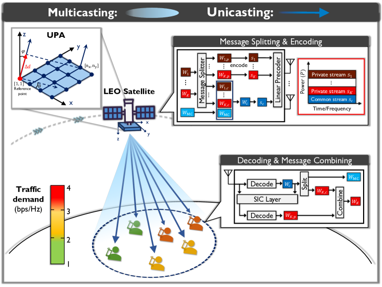
Figure 1: System model of the proposed RSMA-based NOUM transmission.

II-A Satellite Channel Model

To characterize a satellite channel, a widely adopted ray-tracing-based model is employed. The received baseband signal at the $k$-th user from the $(n_{x},n_{y})$-th antenna, in the absence of noise, can be expressed as

$$y_{k}^{[n_{x},n_{y}]}(t)= \sum_{l=0}^{L_{k}-1}\alpha_{k,l}\cdot x(t-\tau_{k,l}^{[n_{x},n_{y}]})$$

$$\times\exp(-j2\pi f_{\sf{c}}\tau_{k,l}^{[n_{x},n_{y}]})\cdot\exp(j2\pi f^{\sf{D}}_{k,l}t),$$ (1)

where $L_{k}$, $\alpha_{k,l}$, and $f_{\sf{c}}$ denote the number of propagation paths, path attenuation over the $l$-th path, and a carrier frequency, respectively. $\tau_{k,l}^{[n_{x},n_{y}]}$ is the propagation delay from the $(n_{x},n_{y})$-th antenna to the $k$-th user over the $l$-th path. $x(t-\tau_{k,l}^{[n_{x},n_{y}]})$ is the transmitted signal from the $(n_{x},n_{y})$-th antenna delayed by $\tau_{k,l}^{[n_{x},n_{y}]}$. $f^{\sf{D}}_{k,l}$ indicates the Doppler shift over the $l$-th propagation path. Without loss of generality, the propagation delays are sorted in the ascending order, such that $\tau_{k,0}^{[n_{x},n_{y}]}\leq\cdots\leq\tau_{k,L_{k}-1}^{[n_{x},n_{y}]}$.

Due to the high altitude of the LEO satellite, LEO SATCOM typically operates under channel conditions dominated by line-of-sight (LOS) components. This feature results in a much smaller delay spread compared to conventional terrestrial networks, as measured in [24, 25]. Therefore, $x(t-\tau_{k,l}^{[n_{x},n_{y}]})$ can be approximated as $x(t-\tau_{k,l}^{[n_{x},n_{y}]})\approx x(t-\tau_{k,0}^{[n_{x},n_{y}]})$, $\forall l$, reformulating (II-A) into

$$y_{k}^{[n_{x},n_{y}]}(t)=h_{k}^{[n_{x},n_{y}]}(t)\cdot x(t-\tau_{k,0}^{[n_{x},n_{y}]}),$$ (2)

where $h_{k}^{[n_{x},n_{y}]}(t)$ is the channel between the $k$-th user and the $(n_{x},n_{y})$-th antenna, given by

$$h_{k}^{[n_{x},n_{y}]}(t)\!=\!\! \sum_{l=0}^{L_{k}-1}\!\alpha_{k,l}\cdot\exp\left(-j2\pi\{f_{\sf{c}}\tau_{k,l}^{[n_{x},n_{y}]}\!-\!f^{\sf{D}}_{k,l}t\}\right).$$ (3)

In (3), the propagation delay from the $(n_{x},n_{y})$-th antenna to the $k$-th user over the $l$-th path can be rewritten as

$$\tau_{k,l}^{[n_{x},n_{y}]}=\tau_{k,l}^{[1,1]}+\Delta\tau^{[n_{x},n_{y}]}(\theta_{k,l},\varphi_{k,l}),$$ (4)

where $\tau_{k,l}^{[1,1]}$ is the propagation delay from the reference point to the $k$-th user over the $l$-th path as shown in Fig. 1. $\Delta\tau^{[n_{x},n_{y}]}(\theta_{k,l},\varphi_{k,l})$ is the time difference of arrival (TDoA) between the reference point and the $(n_{x},n_{y})$-th antenna. $(\theta_{k,l},\varphi_{k,l})$ is angle-of-departure (AoD) pair of the $k$-th user over the $l$-th path, where $\theta_{k,l}$ and $\varphi_{k,l}$ are the azimuth and off-nadir angles. Owing to the high altitude of the LEO satellite, the angle of multiple propagation paths for a certain user can be assumed to be identical, i.e., $\Delta\tau^{[n_{x},n_{y}]}(\theta_{k,l},\varphi_{k,l})\approx\Delta\tau^{[n_{x},n_{y}]}(\theta_{k},\varphi_{k})$, $\forall l$ [7]. Accordingly, (3) is reformulated as

$$h_{k}^{[n_{x},n_{y}]}(t) =\sum_{l=0}^{L_{k}-1}\alpha_{k,l}\cdot\exp\left(-j2\pi\left\{f_{\sf{c}}\tau_{k,l}^{[1,1]}-f^{\sf{D}}_{k,l}t\right\}\right)$$

$$\,\,\,\,\,\,\,\times\exp\left(-j2\pi f_{\sf{c}}\cdot\Delta\tau^{[n_{x},n_{y}]}(\theta_{k},\varphi_{k})\right).$$ (5)

Then, with $\tau_{k,0}^{[1,1]}=\min_{l}{\tau_{k,l}^{[1,1]}}$, (II-A) can be rewritten as

$$h_{k}^{[n_{x},n_{y}]}(t)= \sum_{l=0}^{L_{k}-1}\alpha_{k,l}\cdot\exp\left(-j2\pi\left\{f_{\sf{c}}\tau_{k,0}^{[1,1]}-f^{\sf{D}}_{k,l}t\right\}\right)$$

$$\times\exp\left(-j2\pi\left\{f_{\sf{c}}\left(\tau^{[1,1]}_{k,l}-\tau^{[1,1]}_{k,0}\right)\right\}\right)$$

$$\times\exp\left(-j2\pi f_{\sf{c}}\cdot\Delta\tau^{[n_{x},n_{y}]}(\theta_{k},\varphi_{k})\right).$$ (6)

Given the movement of the LEO satellite and user, $f^{\sf{D}}_{k,l}$ is composed of two independent Doppler shifts arising from the mobility of the LEO satellite $(f^{\sf{D}}_{k,l})^{\sf{sat}}$ and the user $(f^{\sf{D}}_{k,l})^{\sf{user}}$, such that $f^{\sf{D}}_{k,l}=(f^{\sf{D}}_{k,l})^{\sf{sat}}+(f^{\sf{D}}_{k,l})^{\sf{user}}$[7]. It is rational to assume identical $(f^{\sf{D}}_{k,l})^{\sf{sat}}$ across multiple propagation paths, i.e., $(f^{\sf{D}}_{k,l})^{\sf{sat}}=(f^{\sf{D}}_{k})^{\sf{sat}},\forall l$ due to the high altitude of the LEO satellite [7]. Thus, the equation (II-A) can be rewritten as

$$h_{k}^{[n_{x},n_{y}]}(t)= \exp\left(-j2\pi\left\{f_{\sf{c}}\tau_{k,0}^{[1,1]}-(f^{\sf{D}}_{k})^{\sf{sat}}t\right\}\right)$$

$$\times g_{k}(t)\cdot a^{[n_{x},n_{y}]}(\theta_{k},\varphi_{k}),$$ (7)

where $g_{k}(t)$ and $a^{[n_{x},n_{y}]}(\theta_{k},\varphi_{k})$ are respectively defined as

$$\!\!\!g_{k}(t)\!\triangleq\!\!$$

$$\!\!\!\sum_{l=0}^{L_{k}-1}\!\alpha_{k,l}\!\cdot\exp\!\left(-j2\pi\!\left\{f_{\sf{c}}\left(\tau^{[1,1]}_{k,l}\!-\!\tau^{[1,1]}_{k,0}\right)\!-\!(f^{\sf{D}}_{k,l})^{\sf{user}}t\right\}\right),$$ (8)

$$\!\!\!a^{[n_{x},n_{y}]}(\theta_{k},\varphi_{k})\triangleq\exp\left(-j2\pi f_{\sf{c}}\cdot\Delta\tau^{[n_{x},n_{y}]}(\theta_{k},\varphi_{k})\right).$$ (9)

In the equation (9), the TDoA between the reference point and the $(n_{x},n_{y})$-th antenna can be derived by calculating the propagation distance difference between the reference point and the $(n_{x},n_{y})$-th antenna, $\Delta d^{[n_{x},n_{y}]}(\theta_{k},\varphi_{k})$, as follows:

$$\Delta\tau^{[n_{x},n_{y}]}(\theta_{k},\varphi_{k})=\frac{\Delta d^{[n_{x},n_{y}]}(\theta_{k},\varphi_{k})}{c}$$

$$=\frac{\sin\varphi_{k}[(n_{x}-1)d_{x}\sin\theta_{k}+(n_{y}-1)d_{y}\cos\theta_{k}]}{c},$$ (10)

where $c$ denotes the speed of light [26]. Therefore, the equation (9) can be rewritten as

$$a^{[n_{x},n_{y}]}(\theta_{k},\varphi_{k})$$

$$=\exp(-j\frac{2\pi}{\lambda}\sin\varphi_{k}[(n_{x}\!-\!1)d_{x}\sin\theta_{k}+(n_{y}\!-\!1)d_{y}\cos\theta_{k}])$$

$$\overset{(a)}{=}\exp(-j\pi\sin\varphi_{k}[(n_{x}\!-\!1)\sin\theta_{k}+(n_{y}\!-\!1)\cos\theta_{k}]),$$ (11)

where $(a)$ follows from the half-wavelength antenna spacing, i.e., $d_{x}=d_{y}=\frac{\lambda}{2}$. The array response vector of the $k$-th user $\mathbf{a}_{k}$, which is a stacked version of $a^{[n_{x},n_{y}]}(\theta_{k},\varphi_{k})$, can be represented using the Kronecker product as follows:

$$\mathbf{a}_{k}=\mathbf{a}_{k}^{x}\otimes\mathbf{a}_{k}^{y}\in\mathbb{C}^{N_{\sf{t}}\times 1}.$$ (12)

In (12), $\mathbf{a}_{k}^{x}\in\mathbb{C}^{N_{\sf{t}}^{x}\times 1}$ and $\mathbf{a}_{k}^{y}\in\mathbb{C}^{N_{\sf{t}}^{y}\times 1}$ respectively indicate

$$\mathbf{a}_{k}^{x}\triangleq\left[1,e^{-j\pi\sin\varphi_{k}\cos\theta_{k}},\cdots,e^{-j\pi\left(N_{\sf{t}}^{x}-1\right)\sin\varphi_{k}\cos\theta_{k}}\right]^{\sf T},$$

$$\mathbf{a}_{k}^{y}\triangleq\left[1,e^{-j\pi\sin\varphi_{k}\sin\theta_{k}},\cdots,e^{-j\pi\left(N_{\sf{t}}^{y}-1\right)\sin\varphi_{k}\sin\theta_{k}}\right]^{\sf T}.$$

Therefore, the channel vector of the $k$-th user is given by

$$\mathbf{h}_{k}(t)\!=\exp\left(-j2\pi f_{\sf{c}}\left\{\tau_{k,0}^{[1,1]}-(f^{\sf{D}}_{k})^{\sf{sat}}\right\}\right)\cdot g_{k}(t)\cdot\mathbf{a}_{k}.$$ (13)

In (13), $\tau_{k,0}^{[1,1]}$ and $(f^{\sf{D}}_{k})^{\sf{sat}}$ can be compensated with proper time and frequency synchronization as depicted in [7, 27, 28, 29]. Hence, the channel expression (13) can be rewritten as

$$\mathbf{h}_{k}(t)=g_{k}(t)\cdot\mathbf{a}_{k}\in\mathbb{C}^{{N_{\sf{t}}}\times{1}}.$$ (14)

In (14), it can be observed that the statistical properties of the channel are primarily determined by the propagation environment vicinity users. Moreover, $g_{k}(t)$ can be postulated to conform to the Rician fading owing to the favorable LOS condition of LEO SATCOM. From such features, the real and imaginary parts of $g_{k}(t)$ exhibit to follow an independent and identically distributed (i.i.d.) Gaussian distribution such that ${\sf{Re}}\{g_{k}(t)\},{\sf{Im}}\{g_{k}(t)\}\sim\mathcal{N}\left(\sqrt{\frac{\kappa_{k}\gamma_{k}}{2(\kappa_{k}+1)}},\frac{\gamma_{k}}{2(\kappa_{k}+1)}\right)$ with the Rician K-factor $\kappa_{k}$. The average channel power is set as

$$\mathbb{E}\left[|g_{k}(t)|^{2}\right]=\gamma_{k}=\frac{G_{\sf{Tx}}{G_{\sf Rx}}}{(4\pi{f_{\sf{c}}}{d_{k}}/{c})^{2}k_{\sf{B}}{T_{\sf sys}}{B}},$$ (15)

where $G_{\sf Tx}$, $G_{\sf Rx}$, $d_{k}$, $k_{\sf{B}}$, $T_{\sf sys}$, and $B$ denote the transmit antenna gain, user terminal antenna gain, satellite-to-$k$-th user distance, Boltzmann constant, system noise temperature, and bandwidth, respectively. Given the severe propagation delay and short channel coherence time of LEO SATCOM, obtaining instantaneous CSIT is usually infeasible. Instead, we presume that the geometry relations of the satellite-to-users (i.e., $\theta_{k}$, $\varphi_{k}$, $\forall k\in\mathcal{K}$) and the statistical information of channel gain (i.e., $\mathbb{E}\left[|g_{k}(t)|^{2}\right]=\gamma_{k}$, $\forall k\in\mathcal{K}$), which vary comparably slower, are available at the LEO satellite [7, 30, 27, 28, 29]. Since we focus on investigating the system within a certain fading block, we rewrite the channel vector (14) as $\mathbf{h}_{k}=g_{k}\mathbf{a}_{k}$ from the following subsection onwards.

II-B Signal Model for RSMA-Based NOUM Transmission

With a rate-splitting strategy for NOUM transmission, unicast messages of each user $W_{1},\cdots,W_{K}$ are firstly split into common and private parts as $W_{k}\rightarrow\{W_{k,{\sf{c}}},\,\,W_{k,{\sf{p}}}\}$, $\forall k\in\mathcal{K}$. The common messages $W_{1,{\sf{c}}},\cdots,W_{K,{\sf{c}}}$ and multicast message $W_{\sf{mc}}$ are combined into one common message $W_{\sf{c}}$ and then encoded into a common stream $s_{\sf{c}}$ using a codebook that is known by all users. On the other hand, the private messages are encoded into private streams $s_{1},\cdots,s_{K}$ intended for each user, using the dedicated codebooks. Through the precoding vectors $\mathbf{f}_{\sf{c}},\mathbf{f}_{1},\cdots,\mathbf{f}_{K}\in\mathbb{C}^{{N_{\sf{t}}}\times{1}}$, the stream vector $\mathbf{s}=[s_{\sf{c}},s_{1},\cdots,s_{K}]^{\sf{T}}\in\mathbb{C}^{{(K+1)}\times{1}}$ is linearly combined as

$$\mathbf{x}=\mathbf{f}_{\sf{c}}s_{\sf{c}}+\sum_{j=1}^{K}{\mathbf{f}_{j}s_{j}}\in\mathbb{C}^{{N_{\sf{t}}}\times{1}},$$ (16)

where $s_{\sf{c}}$ and $s_{k}$ follow an i.i.d. Gaussian distribution such that $s_{\sf{c}},s_{k}\sim\mathcal{CN}{(0,P)}$. The transmit power constraint is presented as $\|\mathbf{f}_{\sf{c}}\|^{2}+\sum_{j=1}^{K}\|\mathbf{f}_{j}\|^{2}\leq 1$, whereby the total transmit power is constrained by $P$. Then, the received signal at the $k$-th user is represented as

$$y_{k}=\mathbf{h}_{k}^{\sf{H}}\mathbf{x}+n_{k}=\left(g_{k}\mathbf{a}_{k}\right)^{\sf{H}}\bigg{(}\mathbf{f}_{\sf{c}}s_{\sf{c}}+\sum_{j=1}^{K}{\mathbf{f}_{j}s_{j}}\bigg{)}+n_{k},$$ (17)

where $n_{k}$ is the additive white Gaussian noise (AWGN) that follows i.i.d. such that $n_{k}\sim\mathcal{CN}{(0,\sigma_{n}^{2})}$, $\forall k\in\mathcal{K}$. At the receiver, the common stream $s_{\sf{c}}$ is first decoded by treating private streams as noise. After the successful decoding, the data is re-encoded to subtract it from $y_{k}$ via SIC operation. After the SIC, the corresponding private stream is decoded while treating the other private streams as noise.

To design a robust RSMA precoder for NOUM transmission under imperfect CSIT, we characterize the ergodic rate function of instantaneous common and private rates at the $k$-th user as $R_{{\sf{c}},k}=\mathbb{E}[R_{{\sf{c}},k}^{\sf{ins}}]$ and $R_{{\sf{p}},k}=\mathbb{E}[R_{{\sf{p}},k}^{\sf{ins}}]$, respectively. However, since the ergodic rate is usually challenging to handle due to the absence of a general closed form, we derive an upper bound of the ergodic rate as follows:

$$\!\!\!R_{{\sf{c}},k} =\mathbb{E}[R_{{\sf{c}},k}^{\sf{ins}}]=\mathbb{E}\Bigg{[}\log_{2}\Bigg{(}1+\frac{|\mathbf{h}_{k}^{\sf{H}}\mathbf{f}_{\sf{c}}|^{2}}{\sum_{j=1}^{K}|\mathbf{h}_{k}^{\sf{H}}\mathbf{f}_{j}|^{2}+\frac{\sigma_{n}^{2}}{P}}\Bigg{)}\Bigg{]}$$

$$=\mathbb{E}\Bigg{[}\log_{2}\Bigg{(}1+\frac{|g_{k}|^{2}|\mathbf{a}_{k}^{\sf{H}}\mathbf{f}_{\sf{c}}|^{2}}{\sum_{j=1}^{K}|g_{k}|^{2}|\mathbf{a}_{k}^{\sf{H}}\mathbf{f}_{j}|^{2}+\frac{\sigma_{n}^{2}}{P}}\Bigg{)}\Bigg{]}$$

$$\overset{(b)}{\leq}\log_{2}\Bigg{(}1+\frac{\mathbb{E}\left[|g_{k}|^{2}\right]|\mathbf{a}_{k}^{\sf{H}}\mathbf{f}_{\sf{c}}|^{2}}{\sum_{j=1}^{K}\mathbb{E}\left[|g_{k}|^{2}\right]|\mathbf{a}_{k}^{\sf{H}}\mathbf{f}_{j}|^{2}+\frac{\sigma_{n}^{2}}{P}}\Bigg{)}$$

$$\overset{(c)}{=}\log_{2}\Bigg{(}1+\frac{\gamma_{k}|\mathbf{a}_{k}^{\sf{H}}\mathbf{f}_{\sf{c}}|^{2}}{\sum_{j=1}^{K}\gamma_{k}|\mathbf{a}_{k}^{\sf{H}}\mathbf{f}_{j}|^{2}+\frac{\sigma_{n}^{2}}{P}}\Bigg{)}\!=\!\bar{R}_{{\sf{c}},k},$$ (18)

where the step $(b)$ follows from the Jensen’s inequality, i.e., $\log_{2}(1+\frac{a\mathbb{E}[X]}{b\mathbb{E}[X]+c})\geq\mathbb{E}[\log_{2}(1+\frac{aX}{bX+c})]$, due to the concavity of $\log_{2}(1+\frac{aX}{bX+c})$ in terms of $X\geq 0$ for given non-negative numbers of $a$, $b$, and $c$. Step $(c)$ follows from the statistical information of the complex channel gain that is assumed to be known at the LEO satellite. In order to ensure that all users are capable of decoding the common stream, we define a common rate as $\min_{k\in\mathcal{K}}\bar{R}_{{\sf c},k}\triangleq\sum_{j=1}^{K}C_{j}+C_{\sf{mc}}$ in which $C_{k}$ and $C_{\sf{mc}}$ are portions of the common rate allocated to the $k$-th user’s unicast message and the multicast message.

Similarly, the upper bound of $R_{{\sf{p}},k}$ is derived as follows:

$$\!\!\!R_{{\sf{p}},k} =\mathbb{E}[R_{{\sf{p}},k}^{\sf{ins}}]=\mathbb{E}\Bigg{[}\log_{2}\Bigg{(}1+\frac{|\mathbf{h}_{k}^{\sf{H}}\mathbf{f}_{k}|^{2}}{\sum_{j=1,j\neq k}^{K}|\mathbf{h}_{k}^{\sf{H}}\mathbf{f}_{j}|^{2}+\frac{\sigma_{n}^{2}}{P}}\Bigg{)}\Bigg{]}$$

$$=\mathbb{E}\Bigg{[}\log_{2}\Bigg{(}1+\frac{|g_{k}|^{2}|\mathbf{a}_{k}^{\sf{H}}\mathbf{f}_{k}|^{2}}{\sum_{j=1,j\neq k}^{K}|g_{k}|^{2}|\mathbf{a}_{k}^{\sf{H}}\mathbf{f}_{j}|^{2}+\frac{\sigma_{n}^{2}}{P}}\Bigg{)}\Bigg{]}$$

$$\leq\log_{2}\Bigg{(}1+\frac{\mathbb{E}\left[|g_{k}|^{2}\right]|\mathbf{a}_{k}^{\sf{H}}\mathbf{f}_{k}|^{2}}{\sum_{j=1,j\neq k}^{K}\mathbb{E}\left[|g_{k}|^{2}\right]|\mathbf{a}_{k}^{\sf{H}}\mathbf{f}_{j}|^{2}+\frac{\sigma_{n}^{2}}{P}}\Bigg{)}$$

$$=\log_{2}\Bigg{(}1+\frac{\gamma_{k}|\mathbf{a}_{k}^{\sf{H}}\mathbf{f}_{k}|^{2}}{\sum_{j=1,j\neq k}^{K}\gamma_{k}|\mathbf{a}_{k}^{\sf{H}}\mathbf{f}_{j}|^{2}+\frac{\sigma_{n}^{2}}{P}}\Bigg{)}\!=\!\bar{R}_{{\sf{p}},k}.$$ (19)

II-C Problem Formulation

The main objective of this work is to match the offered rates to the non-uniform traffic demands for an efficient superimposed unicast and multicast transmission at the LEO satellite, which typically has a limited power budget. To this end, we formulate an optimization problem to jointly find optimal precoding vectors $\mathbf{f}_{\sf{c}},\mathbf{f}_{1},\cdots,\mathbf{f}_{K}$ and common rate portions $C_{1},\cdots,C_{K},C_{\sf{mc}}$ that minimize the disparity between traffic demands and offered rates as follows:

$$\mathscr{P}_{1}:\,\,\,\,\operatorname*{minimize}_{\mathbf{f}_{\sf{c}},\mathbf{f}_{1},\cdots,\mathbf{f}_{K},\mathbf{c},C_{\sf{mc}}}\,\, \sum_{j=1}^{K}|R_{{\sf target}{,j}}-(C_{j}+\bar{R}_{{\sf{p}},j})|^{2}$$

$$+\eta_{\sf{mc}}|R_{\sf{target,mc}}-C_{\sf{mc}}|^{2}$$

$$\mathrm{s.t.}\,\,\,\,\,\, \min_{k\in\mathcal{K}}\bar{R}_{{\sf c},k}\triangleq\sum_{j=1}^{K}C_{j}+C_{\sf{mc}},$$ (20a)

$$C_{k}\geq 0,\,\,\forall k\in\mathcal{K},\,\,C_{\sf{mc}}\geq 0,$$ (20b)

$$\|\mathbf{f}_{\sf{c}}\|^{2}+\sum\limits_{j=1}^{K}\|\mathbf{f}_{j}\|^{2}\leq 1,$$ (20c)

where $R_{{\sf target}{,k}}$ and $R_{\sf target,mc}$ denote the traffic demands of the unicast message for the $k$-th user and the multicast message, respectively. $\mathbf{c}=[C_{1},\cdots,C_{K}]^{\sf{T}}$ indicates a vector consisting of common rate portions associated with unicast messages, and $\eta_{\sf{mc}}$ indicates a regularization parameter. The constraint (20a) enables $s_{\sf{c}}$ to be decodable by all users, and the constraint (20b) ensures the common rate portions are non-negative values. The transmit power is constrained by (20c).

Remark 1.

(Difference from sum-rate maximization problem with QoS constraints [19, 20]): In the sum rate maximization problem with QoS constraints for unicast and multicast rates, a feasible solution is not always guaranteed. In other words, satisfying demands with QoS constraints can lead to an infeasible solution if the usable power budget is insufficient or the channel condition is unfavorable, thereby reducing communication reliability in LEO satellite networks with power-hungry payloads. In contrast, a feasible solution is always guaranteed in the proposed rate-matching framework regardless of the usable power budget and channel condition.

III Proposed RSMA-Based Rate-Matching Framework for NOUM Transmission

The formulated problem $\mathscr{P}_{1}$ is challenging to solve due to its non-convexity and non-smoothness properties. To tackle this, we convert it into a more tractable form by transforming the constrained problem into an unconstrained problem in which the objective function is differentiable. We then derive the first-order KKT condition of the reformulated problem and show that the first-order KKT condition is cast as an NEPv. Subsequently, we introduce the GPI-RS-NOUM algorithm, based on the principle of the conventional power iteration, to jointly find an optimal rate-matching precoding vector (including power allocation) and common rate portion.

III-A Reformulate the Problem to a Tractable Form

We first reformulate the rate expressions (II-B) and (II-B) as

$$\bar{R}_{{\sf{c}},k} =\log_{2}\Bigg{(}\frac{\sum_{j\in\mathcal{L}}\gamma_{k}|\mathbf{a}_{k}^{\sf{H}}\mathbf{f}_{j}|^{2}+\frac{\sigma_{n}^{2}}{P}}{\sum_{j=1}^{K}\gamma_{k}|\mathbf{a}_{k}^{\sf{H}}\mathbf{f}_{j}|^{2}+\frac{\sigma_{n}^{2}}{P}}\Bigg{)}$$

$$=\log_{2}\Bigg{(}\frac{\sum_{j\in\mathcal{L}}\mathbf{f}_{j}^{\sf{H}}(\gamma_{k}\mathbf{a}_{k}\mathbf{a}_{k}^{\sf{H}})\mathbf{f}_{j}+\frac{\sigma_{n}^{2}}{P}}{\sum_{j=1}^{K}\mathbf{f}_{j}^{\sf{H}}(\gamma_{k}\mathbf{a}_{k}\mathbf{a}_{k}^{\sf{H}})\mathbf{f}_{j}+\frac{\sigma_{n}^{2}}{P}}\Bigg{)},$$ (21)

and

$$\bar{R}_{{\sf{p}},k} =\log_{2}\Bigg{(}\frac{\sum_{j=1}^{K}\gamma_{k}|\mathbf{a}_{k}^{\sf{H}}\mathbf{f}_{j}|^{2}+\frac{\sigma_{n}^{2}}{P}}{\sum_{j=1}^{K}\gamma_{k}|\mathbf{a}_{k}^{\sf{H}}\mathbf{f}_{j}|^{2}+\frac{\sigma_{n}^{2}}{P}}\Bigg{)}$$

$$=\log_{2}\Bigg{(}\frac{\sum_{j=1}^{K}\mathbf{f}_{j}^{\sf{H}}(\gamma_{k}\mathbf{a}_{k}\mathbf{a}_{k}^{\sf{H}})\mathbf{f}_{j}+\frac{\sigma_{n}^{2}}{P}}{\sum_{j=1,j\neq k}^{K}\mathbf{f}_{j}^{\sf{H}}(\gamma_{k}\mathbf{a}_{k}\mathbf{a}_{k}^{\sf{H}})\mathbf{f}_{j}+\frac{\sigma_{n}^{2}}{P}}\Bigg{)},$$ (22)

respectively in which $\mathcal{L}\triangleq\{{\sf{c}},1,\cdots,K\}$. Subsequently, by stacking the precoding vectors as $\bar{\mathbf{f}}=[\mathbf{f}_{\sf{c}}^{\sf{T}},\mathbf{f}_{1}^{\sf{T}},\cdots,\mathbf{f}_{K}^{\sf{T}}]^{\sf{T}}\in\mathbb{C}^{N_{\sf{t}}(K+1)\times 1}$, the numerator term of (III-A) is reformulated as

$$\sum\limits_{j\in\mathcal{L}}\mathbf{f}_{j}^{\sf{H}}(\gamma_{k}\mathbf{a}_{k}\mathbf{a}_{k}^{\sf{H}})\mathbf{f}_{j}+\frac{\sigma_{n}^{2}}{P}=\bar{\mathbf{f}}^{\sf{H}}\mathbf{A}_{k}^{\sf{c}}\bar{\mathbf{f}},$$ (23)

where

$$\mathbf{A}_{k}^{\sf{c}}={\sf{blkdiag}}\left(\gamma_{k}\mathbf{a}_{k}\mathbf{a}_{k}^{\sf{H}},\cdots,\gamma_{k}\mathbf{a}_{k}\mathbf{a}_{k}^{\sf{H}}\right)+\frac{\sigma_{n}^{2}}{P}\mathbf{I},$$ (24)

whose size is ${N_{\sf{t}}(K+1)\times N_{\sf{t}}(K+1)}$. We here assume $\|\bar{\mathbf{f}}\|^{2}=1$. With the similar manner, the denominator term of (III-A) is rewritten as

$$\sum\limits_{j=1}^{K}\mathbf{f}_{j}^{\sf{H}}(\gamma_{k}\mathbf{a}_{k}\mathbf{a}_{k}^{\sf{H}})\mathbf{f}_{j}+\frac{\sigma_{n}^{2}}{P}=\bar{\mathbf{f}}^{\sf{H}}\mathbf{B}_{k}^{\sf{c}}\bar{\mathbf{f}},$$ (25)

where

$$\mathbf{B}_{k}^{\sf{c}}=\mathbf{A}_{k}^{\sf{c}}-{\sf{blkdiag}}\left(\gamma_{k}\mathbf{a}_{k}\mathbf{a}_{k}^{\sf{H}},0,\cdots,0\right),$$ (26)

whose size is ${N_{\sf{t}}(K+1)\times N_{\sf{t}}(K+1)}$. The numerator term of (III-A) is reformulated as

$$\sum\limits_{j=1}^{K}\mathbf{f}_{j}^{\sf{H}}(\gamma_{k}\mathbf{a}_{k}\mathbf{a}_{k}^{\sf{H}})\mathbf{f}_{j}+\frac{\sigma_{n}^{2}}{P}=\bar{\mathbf{f}}^{\sf{H}}\mathbf{A}_{k}^{\sf{p}}\bar{\mathbf{f}},$$ (27)

where

$$\!\!\!\mathbf{A}_{k}^{\sf{p}}\!=\!{\sf{blkdiag}}\left(0,\gamma_{k}\mathbf{a}_{k}\mathbf{a}_{k}^{\sf{H}},\cdots,\gamma_{k}\mathbf{a}_{k}\mathbf{a}_{k}^{\sf{H}}\right)+\frac{\sigma_{n}^{2}}{P}\mathbf{I},$$ (28)

whose size is ${N_{\sf{t}}(K+1)\times N_{\sf{t}}(K+1)}$. Also, the denominator term of (III-A) can be given by

$$\sum\limits_{j=1,j\neq k}^{K}\mathbf{f}_{j}^{\sf{H}}(\gamma_{k}\mathbf{a}_{k}\mathbf{a}_{k}^{\sf{H}})\mathbf{f}_{j}+\frac{\sigma_{n}^{2}}{P}=\bar{\mathbf{f}}^{\sf{H}}\mathbf{B}_{k}^{\sf{p}}\bar{\mathbf{f}},$$ (29)

where

$$\!\!\!\mathbf{B}_{k}^{\sf{p}}=\mathbf{A}_{k}^{\sf{p}}-{\sf{blkdiag}}\bigg{(}0,\cdots,0,\!\underbrace{\gamma_{k}\mathbf{a}_{k}\mathbf{a}_{k}^{\sf{H}}}_{(k+1)\textrm{th block}},0,\cdots,0\bigg{)},$$ (30)

whose size is ${N_{\sf{t}}(K+1)\times N_{\sf{t}}(K+1)}$. By doing so, the equations (III-A) and (III-A) can be reformulated as

$$\bar{R}_{{\sf{c}},k}=\log_{2}\left(\frac{\bar{\mathbf{f}}^{\sf{H}}\mathbf{A}_{k}^{\sf{c}}\bar{\mathbf{f}}}{\bar{\mathbf{f}}^{\sf{H}}\mathbf{B}_{k}^{\sf{c}}\bar{\mathbf{f}}}\right),\,\,\bar{R}_{{\sf{p}},k}=\log_{2}\left(\frac{\bar{\mathbf{f}}^{\sf{H}}\mathbf{A}_{k}^{\sf{p}}\bar{\mathbf{f}}}{\bar{\mathbf{f}}^{\sf{H}}\mathbf{B}_{k}^{\sf{p}}\bar{\mathbf{f}}}\right),$$ (31)

respectively. Therefore, $\mathscr{P}_{1}$ can be reformulated as follows:

$$\mathscr{P}_{2}:\,\,\,\,\operatorname*{minimize}_{\bar{\mathbf{f}},\mathbf{c},C_{\sf{mc}}}\,\, \sum_{j=1}^{K}\left|R_{{\sf target}{,j}}-\left(C_{j}+\log_{2}\left(\frac{\bar{\mathbf{f}}^{\sf{H}}\mathbf{A}_{j}^{\sf{p}}\bar{\mathbf{f}}}{\bar{\mathbf{f}}^{\sf{H}}\mathbf{B}_{j}^{\sf{p}}\bar{\mathbf{f}}}\right)\right)\right|^{2}$$

$$+\eta_{\sf{mc}}|R_{\sf{target,mc}}-C_{\sf{mc}}|^{2}$$

$$\mathrm{s.t.}\,\,\,\,\,\, \min_{k\in\mathcal{K}}\,\,\log_{2}\left(\frac{\bar{\mathbf{f}}^{\sf{H}}\mathbf{A}_{k}^{\sf{c}}\bar{\mathbf{f}}}{\bar{\mathbf{f}}^{\sf{H}}\mathbf{B}_{k}^{\sf{c}}\bar{\mathbf{f}}}\right)\triangleq\sum_{j=1}^{K}C_{j}+C_{\sf{mc}},$$ (32a)

$$C_{k}\geq 0,\,\,\forall k\in\mathcal{K},\,\,C_{\sf{mc}}\geq 0,$$ (32b)

$$\|\bar{\mathbf{f}}\|^{2}=1.$$ (32c)

Note that the transmit power does not affect the value of rate equations as it can always be normalized. In other words, rate expressions are scale invariant with the transmit power. Thus, the constraint (32c) is vanished in $\mathscr{P}_{2}$, reformulating it as

$$\mathscr{P}_{3}:\,\,\,\,\operatorname*{minimize}_{\bar{\mathbf{f}},\mathbf{c},C_{\sf{mc}}}\,\, \sum_{j=1}^{K}\left|R_{{\sf target}{,j}}-\left(C_{j}+\log_{2}\left(\frac{\bar{\mathbf{f}}^{\sf{H}}\mathbf{A}_{j}^{\sf{p}}\bar{\mathbf{f}}}{\bar{\mathbf{f}}^{\sf{H}}\mathbf{B}_{j}^{\sf{p}}\bar{\mathbf{f}}}\right)\right)\right|^{2}$$

$$+\eta_{\sf{mc}}|R_{\sf{target,mc}}-C_{\sf{mc}}|^{2}$$

$$\mathrm{s.t.}\,\,\,\,\,\, \min_{k\in\mathcal{K}}\,\,\log_{2}\left(\frac{\bar{\mathbf{f}}^{\sf{H}}\mathbf{A}_{k}^{\sf{c}}\bar{\mathbf{f}}}{\bar{\mathbf{f}}^{\sf{H}}\mathbf{B}_{k}^{\sf{c}}\bar{\mathbf{f}}}\right)\triangleq\sum_{j=1}^{K}C_{j}+C_{\sf{mc}},$$ (33a)

$$C_{k}\geq 0,\,\,\forall k\in\mathcal{K},\,\,C_{\sf{mc}}\geq 0.$$ (33b)

Subsequently, to make the non-smooth minimum function differentiable, we employ the LogSumExp technique [31] as

$$\!\!\!\!\!\min_{k\in\mathcal{K}}\bar{R}_{{\sf{c}},k}\approx\log\left(\frac{1}{K}\sum_{i=1}^{K}\exp\left\{-\frac{1}{\alpha}\log_{2}\left(\frac{\bar{\mathbf{f}}^{\sf{H}}\mathbf{A}_{i}^{\sf{c}}\bar{\mathbf{f}}}{\bar{\mathbf{f}}^{\sf{H}}\mathbf{B}_{i}^{\sf{c}}\bar{\mathbf{f}}}\right)\right\}\right)^{\!\!-\alpha}\!\!\!\!\!\!,$$ (34)

where the approximation becomes tight as $\alpha\rightarrow+0$. With the approximated equation, the problem $\mathscr{P}_{3}$ can be rewritten as

$$\mathscr{P}_{4}:\,\,\,\,\operatorname*{minimize}_{\bar{\mathbf{f}},\mathbf{c},C_{\sf{mc}}}\,\, \sum_{j=1}^{K}\left|R_{{\sf target}{,j}}-\left(C_{j}+\log_{2}\left(\frac{\bar{\mathbf{f}}^{\sf{H}}\mathbf{A}_{j}^{\sf{p}}\bar{\mathbf{f}}}{\bar{\mathbf{f}}^{\sf{H}}\mathbf{B}_{j}^{\sf{p}}\bar{\mathbf{f}}}\right)\right)\right|^{2}$$

$$+\eta_{\sf{mc}}|R_{\sf{target,mc}}-C_{\sf{mc}}|^{2}$$

$$\mathrm{s.t.}\, \log\left(\frac{1}{K}\sum_{i=1}^{K}\exp\left\{\log_{2}\left(\frac{\bar{\mathbf{f}}^{\sf{H}}\mathbf{A}_{i}^{\sf{c}}\bar{\mathbf{f}}}{\bar{\mathbf{f}}^{\sf{H}}\mathbf{B}_{i}^{\sf{c}}\bar{\mathbf{f}}}\right)^{\!\!\!-\frac{1}{\alpha}}\right\}\right)^{\!\!\!-\alpha}\!\!\!\!\!=\!\sum_{j=1}^{K}C_{j}+C_{\sf{mc}},$$ (35a)

$$\,C_{k}\geq 0,\,\,\forall k\in\mathcal{K},\,\,C_{\sf{mc}}\geq 0.$$ (35b)

Nevertheless, addressing the reformed problem $\mathscr{P}_{4}$ remains a formidable task due to the non-convex constraint (35a) and multiple constraints associated with common rates in (35b). To resolve this issue, we rewrite the common rate portion of the $k$-th user $C_{k}$ into the ratio of the equation (34) as

$$C_{k}(\bar{\mathbf{f}},\mathbf{v})=$$

$$\frac{\mathbf{v}^{\sf{H}}\mathbf{E}_{k}\mathbf{v}}{\mathbf{v}^{\sf{H}}\mathbf{v}}\log\left(\frac{1}{K}\sum_{i=1}^{K}\exp\left\{-\frac{1}{\alpha}\log_{2}\left(\frac{\bar{\mathbf{f}}^{\sf{H}}\mathbf{A}_{i}^{\sf{c}}\bar{\mathbf{f}}}{\bar{\mathbf{f}}^{\sf{H}}\mathbf{B}_{i}^{\sf{c}}\bar{\mathbf{f}}}\right)\right\}\right)^{\!\!-\alpha}\!,$$ (36)

where $\mathbf{v}\in\mathbb{C}^{(K+1)\times 1}$ and $\mathbf{E}_{k}\in\mathbb{C}^{(K+1)\times(K+1)}$ indicate $\mathbf{v}=[v_{1},\cdots,v_{K},v_{K+1}]^{\sf{T}}$ and the diagonal matrix in which the $(k,k)$-th diagonal element is set to be $1$ and otherwise $0$, respectively. Then, $C_{\sf{mc}}$ can be rewritten as

$$\!\!\!C_{\sf{mc}}(\bar{\mathbf{f}},\mathbf{v})=$$

$$\!\!\!\frac{\mathbf{v}^{\sf{H}}\mathbf{E}_{K+1}\mathbf{v}}{\mathbf{v}^{\sf{H}}\mathbf{v}}\log\left(\!\frac{1}{K}\sum_{i=1}^{K}\exp\left\{-\frac{1}{\alpha}\log_{2}\left(\frac{\bar{\mathbf{f}}^{\sf{H}}\mathbf{A}_{i}^{\sf{c}}\bar{\mathbf{f}}}{\bar{\mathbf{f}}^{\sf{H}}\mathbf{B}_{i}^{\sf{c}}\bar{\mathbf{f}}}\right)\right\}\!\right)^{\!\!-\alpha}$$ (37)

into the fractional form. It is noted that the value of $\frac{\mathbf{v}^{\sf{H}}\mathbf{E}_{k}\mathbf{v}}{\mathbf{v}^{\sf{H}}\mathbf{v}}=\frac{v_{k}^{2}}{\sum_{j=1}^{K+1}v_{j}^{2}}$, $\forall$ $k\in\{1,\cdots,K,K+1\}$, is always between $0$ and $1$. In addition to this, the summation for the ratio term of each common stream is $1$, i.e., $\sum_{j=1}^{K+1}{\frac{\mathbf{v}^{\sf{H}}\mathbf{E}_{j}\mathbf{v}}{\mathbf{v}^{\sf{H}}\mathbf{v}}}=1.$ Thanks to these features, the constraints (35a) and (35b) can be vanished from $\mathscr{P}_{4}$. Therefore, $\mathscr{P}_{4}$ can be reformulated into the unconstrained problem as follows:

$$\mathscr{P}_{5}:\operatorname*{minimize}_{\bar{\mathbf{f}},\mathbf{v}}f(\bar{\mathbf{f}},\mathbf{v}),$$ (38)

where

$$f(\bar{\mathbf{f}},\mathbf{v}) =\sum_{j=1}^{K}\left|R_{{\sf target}{,j}}\!-\!\left(\log_{2}\left(\frac{\bar{\mathbf{f}}^{\sf{H}}\mathbf{A}_{j}^{\sf{p}}\bar{\mathbf{f}}}{\bar{\mathbf{f}}^{\sf{H}}\mathbf{B}_{j}^{\sf{p}}\bar{\mathbf{f}}}\right)+C_{j}(\bar{\mathbf{f}},\mathbf{v})\right)\right|^{2}$$

$$+\eta_{\sf{mc}}\left|R_{\sf{target,mc}}-C_{\sf{mc}}(\bar{\mathbf{f}},\mathbf{v})\right|^{2}.$$ (39)

III-B Optimal Precoder Design via GPI-RS-NOUM Algorithm

Although $\mathscr{P}_{5}$ is a unconstrained problem, obtaining optimal $\bar{\mathbf{f}}$ and $\mathbf{v}$ is still challenging due to the non-convexity of $f(\bar{\mathbf{f}},\mathbf{v})$. To resolve this, we derive the first-order KKT condition of $\mathscr{P}_{5}$ to be formulated as an NEPv [32]. The GPI-RS-NOUM algorithm built upon the process of conventional power iteration is introduced to identify the leading eigenvector that maximizes the eigenvalue of the presented NEPv. These procedures are explained step-by-step to improve readability.

Step I) First-order KKT condition w.r.t. $\bar{\mathbf{f}}$

We first derive the first-order KKT condition of the problem (38) with respect to $\bar{\mathbf{f}}$, i.e., $\frac{\partial{f(\bar{\mathbf{f}},\mathbf{v})}}{\partial{\bar{\mathbf{f}}}}=\mathbf{0}$. The following Lemma 1 indicates the first-order KKT condition to $\bar{\mathbf{f}}$.

Lemma 1.

The first-order KKT condition of (38) with respect to $\bar{\mathbf{f}}$ holds when the following equation is satisfied.

$${\mathbf{B}(\bar{\mathbf{f}},\mathbf{v})}^{-1}{\mathbf{A}(\bar{\mathbf{f}},\mathbf{v})}\bar{\mathbf{f}}=\lambda(\bar{\mathbf{f}},\mathbf{v})\bar{\mathbf{f}}.$$ (40)

The matrices ${\mathbf{A}(\bar{\mathbf{f}},\mathbf{v})}$ and ${\mathbf{B}(\bar{\mathbf{f}},\mathbf{v})}$ $\in\mathbb{C}^{N_{\sf{t}}(K+1)\times N_{\sf{t}}(K+1)}$ in the equation (40) are respectively expressed as (1) and (1) at the top of this page with the following equations (43)$-$(47).

$${\mathbf{A}(\bar{\mathbf{f}},\mathbf{v})}=\lambda_{\sf{num}}(\bar{\mathbf{f}},\mathbf{v})\!\times\!\Bigg{\{}\sum_{j=1}^{K}\Bigg{[}R_{{\sf{target}},j}\left(\frac{{\mathbf{A}_{j}^{\sf{p}}}}{\bar{\mathbf{f}}^{\sf{H}}{\mathbf{A}_{j}^{\sf{p}}}{\bar{\mathbf{f}}}}+\frac{\mathbf{v}^{\sf{H}}\mathbf{E}_{j}\mathbf{v}}{\mathbf{v}^{\sf{H}}\mathbf{v}}\mathbf{L}_{\sf{A}}(\bar{\mathbf{f}})\right)+\log_{2}\left(\frac{\bar{\mathbf{f}}^{\sf{H}}\mathbf{A}_{j}^{\sf{p}}\bar{\mathbf{f}}}{\bar{\mathbf{f}}^{\sf{H}}\mathbf{B}_{j}^{\sf{p}}\bar{\mathbf{f}}}\right)\frac{{\mathbf{B}_{j}^{\sf{p}}}}{\bar{\mathbf{f}}^{\sf{H}}{\mathbf{B}_{j}^{\sf{p}}}{\bar{\mathbf{f}}}}+\frac{\mathbf{v}^{\sf{H}}\mathbf{E}_{j}\mathbf{v}}{\mathbf{v}^{\sf{H}}\mathbf{v}}C_{j}(\bar{\mathbf{f}},\mathbf{v})\mathbf{L}_{\sf{B}}(\bar{\mathbf{f}})$$

$$+\frac{\mathbf{v}^{\sf{H}}\mathbf{E}_{j}\mathbf{v}}{\mathbf{v}^{\sf{H}}\mathbf{v}}\log_{2}\left(\frac{\bar{\mathbf{f}}^{\sf{H}}\mathbf{A}_{j}^{\sf{p}}\bar{\mathbf{f}}}{\bar{\mathbf{f}}^{\sf{H}}\mathbf{B}_{j}^{\sf{p}}\bar{\mathbf{f}}}\right)\mathbf{L}_{\sf{B}}(\bar{\mathbf{f}})+C_{j}(\bar{\mathbf{f}},\mathbf{v})\frac{{\mathbf{B}_{j}^{\sf{p}}}}{\bar{\mathbf{f}}^{\sf{H}}{\mathbf{B}_{j}^{\sf{p}}}{\bar{\mathbf{f}}}}\Bigg{]}+\eta_{\sf{mc}}\left[R_{\sf{target,mc}}\frac{\mathbf{v}^{\sf{H}}\mathbf{E}_{K+1}\mathbf{v}}{\mathbf{v}^{\sf{H}}\mathbf{v}}\mathbf{L}_{\sf{A}}(\bar{\mathbf{f}})+\frac{\mathbf{v}^{\sf{H}}\mathbf{E}_{K+1}\mathbf{v}}{\mathbf{v}^{\sf{H}}\mathbf{v}}C_{\sf{mc}}(\bar{\mathbf{f}},\mathbf{v})\mathbf{L}_{\sf{B}}(\bar{\mathbf{f}})\right]\Bigg{\}}.$$ (41)

 

$${\mathbf{B}(\bar{\mathbf{f}},\mathbf{v})}=\lambda_{\sf{den}}(\bar{\mathbf{f}},\mathbf{v})\!\times\!\Bigg{\{}\sum_{j=1}^{K}\Bigg{[}R_{{\sf{target}},j}\left(\frac{{\mathbf{B}_{j}^{\sf{p}}}}{\bar{\mathbf{f}}^{\sf{H}}{\mathbf{B}_{j}^{\sf{p}}}{\bar{\mathbf{f}}}}+\frac{\mathbf{v}^{\sf{H}}\mathbf{E}_{j}\mathbf{v}}{\mathbf{v}^{\sf{H}}\mathbf{v}}\mathbf{L}_{\sf{B}}(\bar{\mathbf{f}})\right)+\log_{2}\left(\frac{\bar{\mathbf{f}}^{\sf{H}}\mathbf{A}_{j}^{\sf{p}}\bar{\mathbf{f}}}{\bar{\mathbf{f}}^{\sf{H}}\mathbf{B}_{j}^{\sf{p}}\bar{\mathbf{f}}}\right)\frac{{\mathbf{A}_{j}^{\sf{p}}}}{\bar{\mathbf{f}}^{\sf{H}}{\mathbf{A}_{j}^{\sf{p}}}{\bar{\mathbf{f}}}}+\frac{\mathbf{v}^{\sf{H}}\mathbf{E}_{j}\mathbf{v}}{\mathbf{v}^{\sf{H}}\mathbf{v}}C_{j}(\bar{\mathbf{f}},\mathbf{v})\mathbf{L}_{\sf{A}}(\bar{\mathbf{f}})$$

$$+\frac{\mathbf{v}^{\sf{H}}\mathbf{E}_{j}\mathbf{v}}{\mathbf{v}^{\sf{H}}\mathbf{v}}\log_{2}\left(\frac{\bar{\mathbf{f}}^{\sf{H}}\mathbf{A}_{j}^{\sf{p}}\bar{\mathbf{f}}}{\bar{\mathbf{f}}^{\sf{H}}\mathbf{B}_{j}^{\sf{p}}\bar{\mathbf{f}}}\right)\mathbf{L}_{\sf{A}}(\bar{\mathbf{f}})+C_{j}(\bar{\mathbf{f}},\mathbf{v})\frac{{\mathbf{A}_{j}^{\sf{p}}}}{\bar{\mathbf{f}}^{\sf{H}}{\mathbf{A}_{j}^{\sf{p}}}{\bar{\mathbf{f}}}}\Bigg{]}+\eta_{\sf{mc}}\left[R_{\sf{target,mc}}\frac{\mathbf{v}^{\sf{H}}\mathbf{E}_{K+1}\mathbf{v}}{\mathbf{v}^{\sf{H}}\mathbf{v}}\mathbf{L}_{\sf{B}}(\bar{\mathbf{f}})+\frac{\mathbf{v}^{\sf{H}}\mathbf{E}_{K+1}\mathbf{v}}{\mathbf{v}^{\sf{H}}\mathbf{v}}C_{\sf{mc}}(\bar{\mathbf{f}},\mathbf{v})\mathbf{L}_{\sf{A}}(\bar{\mathbf{f}})\right]\Bigg{\}}.$$ (42)

 

$$\mathbf{L}_{\sf{A}}(\bar{\mathbf{f}})\!=\!\sum_{i=1}^{K}\left({\frac{\exp\left\{-\frac{1}{\alpha}\log_{2}\left(\frac{\bar{\mathbf{f}}^{\sf{H}}\mathbf{A}_{i}^{\sf{c}}\bar{\mathbf{f}}}{\bar{\mathbf{f}}^{\sf{H}}\mathbf{B}_{i}^{\sf{c}}\bar{\mathbf{f}}}\right)\right\}}{\sum_{\ell=1}^{K}{\exp\left\{-\frac{1}{\alpha}\log_{2}\left(\frac{\bar{\mathbf{f}}^{\sf{H}}\mathbf{A}_{\ell}^{\sf{c}}\bar{\mathbf{f}}}{\bar{\mathbf{f}}^{\sf{H}}\mathbf{B}_{\ell}^{\sf{c}}\bar{\mathbf{f}}}\right)\right\}}}}\cdot\frac{{\mathbf{A}_{i}^{\sf{c}}}}{\bar{\mathbf{f}}^{\sf{H}}{\mathbf{A}_{i}^{\sf{c}}}{\bar{\mathbf{f}}}}\right),$$ (43)

$$\mathbf{L}_{\sf{B}}(\bar{\mathbf{f}})\!=\!\sum_{i=1}^{K}\left({\frac{\exp\left\{-\frac{1}{\alpha}\log_{2}\left(\frac{\bar{\mathbf{f}}^{\sf{H}}\mathbf{A}_{i}^{\sf{c}}\bar{\mathbf{f}}}{\bar{\mathbf{f}}^{\sf{H}}\mathbf{B}_{i}^{\sf{c}}\bar{\mathbf{f}}}\right)\right\}}{\sum_{\ell=1}^{K}{\exp\left\{-\frac{1}{\alpha}\log_{2}\left(\frac{\bar{\mathbf{f}}^{\sf{H}}\mathbf{A}_{\ell}^{\sf{c}}\bar{\mathbf{f}}}{\bar{\mathbf{f}}^{\sf{H}}\mathbf{B}_{\ell}^{\sf{c}}\bar{\mathbf{f}}}\right)\right\}}}}\cdot\frac{{\mathbf{B}_{i}^{\sf{c}}}}{\bar{\mathbf{f}}^{\sf{H}}{\mathbf{B}_{i}^{\sf{c}}}{\bar{\mathbf{f}}}}\right),$$ (44)

$$\lambda(\bar{\mathbf{f}},\mathbf{v})=\exp\left(-\eta_{\sf{mc}}\left|R_{{\sf{target,mc}}}-C_{{\sf{mc}}}(\bar{\mathbf{f}},\mathbf{v})\right|^{2}\right)\times$$

$$\prod_{j=1}^{K}\exp\left(-\left|R_{{\sf{target}},j}-\left(\log_{2}\left(\frac{\bar{\mathbf{f}}^{\sf{H}}\mathbf{A}_{j}^{\sf{p}}\bar{\mathbf{f}}}{\bar{\mathbf{f}}^{\sf{H}}\mathbf{B}_{j}^{\sf{p}}\bar{\mathbf{f}}}\right)+C_{j}(\bar{\mathbf{f}},\mathbf{v})\right)\right|^{2}\right),$$ (45)

$$\lambda_{\sf{num}}(\bar{\mathbf{f}},\mathbf{v})=$$

$$\prod_{j=1}^{K}\exp\left(-\left|R_{{\sf{target}},j}-\left(\log_{2}\left(\frac{\bar{\mathbf{f}}^{\sf{H}}\mathbf{A}_{j}^{\sf{p}}\bar{\mathbf{f}}}{\bar{\mathbf{f}}^{\sf{H}}\mathbf{B}_{j}^{\sf{p}}\bar{\mathbf{f}}}\right)+C_{j}(\bar{\mathbf{f}},\mathbf{v})\right)\right|^{2}\right),$$ (46)

and

$$\lambda_{\sf{den}}(\bar{\mathbf{f}},\mathbf{v})=\exp\left(\eta_{\sf{mc}}\left|R_{{\sf{target,mc}}}-C_{{\sf{mc}}}(\bar{\mathbf{f}},\mathbf{v})\right|^{2}\right),$$ (47)

where $\mathbf{L}_{\sf{A}}(\bar{\mathbf{f}})$ and $\mathbf{L}_{\sf{B}}(\bar{\mathbf{f}})$ $\in\mathbb{C}^{N_{\sf{t}}(K+1)\times N_{\sf{t}}(K+1)}$.

Proof.

Please refer to Appendix A. ∎

Step II) First-order KKT condition w.r.t. ${\mathbf{v}}$

Subsequently, we derive the first-order KKT condition of (38) with respect to ${\mathbf{v}}$, i.e., $\frac{\partial{f(\bar{\mathbf{f}},\mathbf{v})}}{\partial{{\mathbf{v}}}}=\mathbf{0}$. The following Lemma 2 shows the first-order KKT condition to $\mathbf{v}$.

Lemma 2.

The first-order KKT condition of (38) with respect to $\mathbf{v}$ holds when the following equation is satisfied.

$${\mathbf{E}(\bar{\mathbf{f}},\mathbf{v})}^{-1}{\mathbf{D}(\bar{\mathbf{f}},\mathbf{v})}{\mathbf{v}}=\lambda(\bar{\mathbf{f}},\mathbf{v}){\mathbf{v}},$$ (48)

where ${\mathbf{D}(\bar{\mathbf{f}},\mathbf{v})}$ and ${\mathbf{E}(\bar{\mathbf{f}},\mathbf{v})}$ $\in\mathbb{R}^{(K+1)\times(K+1)}$ are respectively presented as (2) and (2) at the top of the next page.

$${\mathbf{D}(\bar{\mathbf{f}},\mathbf{v})}= \lambda_{\sf{num}}(\bar{\mathbf{f}},\mathbf{v})\!\times\!\Bigg{\{}\sum\limits_{j=1}^{K}\Bigg{[}R_{{\sf{target}},j}\frac{\mathbf{E}_{j}}{\mathbf{v}^{\sf{H}}\mathbf{v}}+\log\left(\frac{1}{K}\sum_{i=1}^{K}\exp\left(-\frac{1}{\alpha}\log_{2}\left(\frac{\bar{\mathbf{f}}^{\sf{H}}\mathbf{A}_{i}^{\sf{c}}\bar{\mathbf{f}}}{\bar{\mathbf{f}}^{\sf{H}}\mathbf{B}_{i}^{\sf{c}}\bar{\mathbf{f}}}\right)\right)\right)^{\!\!-\alpha}\!\!\!\!\!\!\cdot\frac{\mathbf{v}^{\sf{H}}\mathbf{E}_{j}\mathbf{v}}{\mathbf{v}^{\sf{H}}\mathbf{v}}\cdot\frac{\mathbf{v}^{\sf{H}}\mathbf{E}_{j}\mathbf{v}}{(\mathbf{v}^{\sf{H}}\mathbf{v})^{2}}\mathbf{I}+\log_{2}\left(\frac{\bar{\mathbf{f}}^{\sf{H}}\mathbf{A}_{j}^{\sf{p}}\bar{\mathbf{f}}}{\bar{\mathbf{f}}^{\sf{H}}\mathbf{B}_{j}^{\sf{p}}\bar{\mathbf{f}}}\right)\frac{\mathbf{v}^{\sf{H}}\mathbf{E}_{j}\mathbf{v}}{(\mathbf{v}^{\sf{H}}\mathbf{v})^{2}}\mathbf{I}\Bigg{]}$$

$$+\eta_{\sf{mc}}\Bigg{[}R_{\sf{target,mc}}\frac{\mathbf{E}_{K+1}}{\mathbf{v}^{\sf{H}}\mathbf{v}}+\log\left(\frac{1}{K}\sum_{i=1}^{K}\exp\left(-\frac{1}{\alpha}\log_{2}\left(\frac{\bar{\mathbf{f}}^{\sf{H}}\mathbf{A}_{i}^{\sf{c}}\bar{\mathbf{f}}}{\bar{\mathbf{f}}^{\sf{H}}\mathbf{B}_{i}^{\sf{c}}\bar{\mathbf{f}}}\right)\right)\right)^{\!\!-\alpha}\!\!\!\!\!\!\cdot\frac{\mathbf{v}^{\sf{H}}\mathbf{E}_{K+1}\mathbf{v}}{\mathbf{v}^{\sf{H}}\mathbf{v}}\cdot\frac{\mathbf{v}^{\sf{H}}\mathbf{E}_{K+1}\mathbf{v}}{(\mathbf{v}^{\sf{H}}\mathbf{v})^{2}}\mathbf{I}\Bigg{]}\Bigg{\}}.$$ (49)

 

$${\mathbf{E}(\bar{\mathbf{f}},\mathbf{v})}= \lambda_{\sf{den}}(\bar{\mathbf{f}},\mathbf{v})\!\times\!\Bigg{\{}\sum\limits_{j=1}^{K}\Bigg{[}R_{{\sf{target}},j}\frac{\mathbf{v}^{\sf{H}}\mathbf{E}_{j}\mathbf{v}}{(\mathbf{v}^{\sf{H}}\mathbf{v})^{2}}\mathbf{I}+\log\left(\frac{1}{K}\sum_{i=1}^{K}\exp\left(-\frac{1}{\alpha}\log_{2}\left(\frac{\bar{\mathbf{f}}^{\sf{H}}\mathbf{A}_{i}^{\sf{c}}\bar{\mathbf{f}}}{\bar{\mathbf{f}}^{\sf{H}}\mathbf{B}_{i}^{\sf{c}}\bar{\mathbf{f}}}\right)\right)\right)^{\!\!-\alpha}\!\!\!\!\!\!\cdot\frac{\mathbf{v}^{\sf{H}}\mathbf{E}_{j}\mathbf{v}}{\mathbf{v}^{\sf{H}}\mathbf{v}}\cdot\frac{\mathbf{E}_{j}}{\mathbf{v}^{\sf{H}}\mathbf{v}}+\log_{2}\left(\frac{\bar{\mathbf{f}}^{\sf{H}}\mathbf{A}_{j}^{\sf{p}}\bar{\mathbf{f}}}{\bar{\mathbf{f}}^{\sf{H}}\mathbf{B}_{j}^{\sf{p}}\bar{\mathbf{f}}}\right)\frac{\mathbf{E}_{j}}{\mathbf{v}^{\sf{H}}\mathbf{v}}\Bigg{]}$$

$$+\eta_{\sf{mc}}\Bigg{[}R_{\sf{target,mc}}\frac{\mathbf{v}^{\sf{H}}\mathbf{E}_{K+1}\mathbf{v}}{(\mathbf{v}^{\sf{H}}\mathbf{v})^{2}}\mathbf{I}+\log\left(\frac{1}{K}\sum_{i=1}^{K}\exp\left(-\frac{1}{\alpha}\log_{2}\left(\frac{\bar{\mathbf{f}}^{\sf{H}}\mathbf{A}_{i}^{\sf{c}}\bar{\mathbf{f}}}{\bar{\mathbf{f}}^{\sf{H}}\mathbf{B}_{i}^{\sf{c}}\bar{\mathbf{f}}}\right)\right)\right)^{\!\!-\alpha}\!\!\!\!\!\!\cdot\frac{\mathbf{v}^{\sf{H}}\mathbf{E}_{K+1}\mathbf{v}}{\mathbf{v}^{\sf{H}}\mathbf{v}}\cdot\frac{\mathbf{E}_{K+1}}{\mathbf{v}^{\sf{H}}\mathbf{v}}\Bigg{]}\Bigg{\}}.$$ (50)

 

Proof.

Please refer to Appendix B. ∎

Step III) First-order KKT condition of $\mathscr{P}_{5}$

By stacking (40) and (48) into a block-diagonal matrix form, the first-order KKT condition of (38) is expressed into the NEPv as

$$\begin{bmatrix}{\mathbf{B}(\bar{\mathbf{f}},\mathbf{v})}^{-1}&\mathbf{0}\\ \mathbf{0}&{\mathbf{E}(\bar{\mathbf{f}},\mathbf{v})}^{-1}\end{bmatrix}\!\!\!\begin{bmatrix}{\mathbf{A}(\bar{\mathbf{f}},\mathbf{v})}&\mathbf{0}\\ \mathbf{0}&{\mathbf{D}(\bar{\mathbf{f}},\mathbf{v})}\end{bmatrix}\!\!\!\begin{bmatrix}\bar{\mathbf{f}}\\ \mathbf{v}\end{bmatrix}\!\!=\lambda(\bar{\mathbf{f}},\mathbf{v})\!\!\begin{bmatrix}\bar{\mathbf{f}}\\ \mathbf{v}\end{bmatrix}$$

$$\Leftrightarrow\mathbf{U}(\bar{\mathbf{f}},\mathbf{v})^{-1}\mathbf{W}(\bar{\mathbf{f}},\mathbf{v})\begin{bmatrix}\bar{\mathbf{f}}\\ \mathbf{v}\end{bmatrix}=\lambda(\bar{\mathbf{f}},\mathbf{v})\begin{bmatrix}\bar{\mathbf{f}}\\ \mathbf{v}\end{bmatrix},$$ (51)

where $[\bar{\mathbf{f}}^{\sf{T}},\mathbf{v}^{\sf{T}}]^{\sf{T}}$, $\mathbf{U}(\bar{\mathbf{f}},\mathbf{v})^{-1}\mathbf{W}(\bar{\mathbf{f}},\mathbf{v})$, and $\lambda(\bar{\mathbf{f}},\mathbf{v})$ are eigenvector, eigenvector-dependent matrix, and eigenvalue, respectively. Herein, $\mathbf{U}(\bar{\mathbf{f}},\mathbf{v})$ and $\mathbf{W}(\bar{\mathbf{f}},\mathbf{v})$ are defined as follows:

$$\begin{bmatrix}{\mathbf{B}(\bar{\mathbf{f}},\mathbf{v})}&\mathbf{0}\\ \mathbf{0}&{\mathbf{E}(\bar{\mathbf{f}},\mathbf{v})}\end{bmatrix}\triangleq\mathbf{U}(\bar{\mathbf{f}},\mathbf{v})\in\mathbb{C}^{N_{\sf{t}}(K+2)\times N_{\sf{t}}(K+2)},$$

$$\begin{bmatrix}{\mathbf{A}(\bar{\mathbf{f}},\mathbf{v})}&\mathbf{0}\\ \mathbf{0}&{\mathbf{D}(\bar{\mathbf{f}},\mathbf{v})}\end{bmatrix}\!\triangleq\mathbf{W}(\bar{\mathbf{f}},\mathbf{v})\in\mathbb{C}^{N_{\sf{t}}(K+2)\times N_{\sf{t}}(K+2)}.$$ (52)

We note that the eigenvalue $\lambda(\bar{\mathbf{f}},\mathbf{v})$ of (III-B) is given by $\exp{\left(-f(\bar{\mathbf{f}},\mathbf{v})\right)}$ in which $f(\bar{\mathbf{f}},\mathbf{v})$ is the objective function for $\mathscr{P}_{5}$. Thus, identifying the leading eigenvector that maximizes the eigenvalue is equivalent to finding the best local optimums $\bar{\mathbf{f}}^{[\star]}$ and $\mathbf{v}^{[\star]}$ that minimize the disparity between the demands and offered rates among the first-order optimal points.

Step IV) GPI-RS-NOUM algorithm

To obtain the best local optima $\bar{\mathbf{f}}^{[\star]}$ and $\mathbf{v}^{[\star]}$ in a computational efficient manner, we propose GPI-RS-NOUM algorithm built upon the method in [33, 34]. We update $\bar{\mathbf{f}}^{[t]}$ and $\mathbf{v}^{[t]}$ at the $t$-th iteration by

$$[(\bar{\mathbf{f}}^{[t]})^{\sf{T}},(\mathbf{v}^{[t]})^{\sf{T}}]^{\sf{T}}\leftarrow$$ (53)

$$\frac{\mathbf{U}(\bar{\mathbf{f}}^{[t-1]},\mathbf{v}^{[t-1]})^{-1}\mathbf{W}(\bar{\mathbf{f}}^{[t-1]},\mathbf{v}^{[t-1]})[(\bar{\mathbf{f}}^{[t-1]})^{\sf{T}},(\mathbf{v}^{[t-1]})^{\sf{T}}]^{\sf{T}}}{\|\mathbf{U}(\bar{\mathbf{f}}^{[t-1]},\mathbf{v}^{[t-1]})^{-1}\mathbf{W}(\bar{\mathbf{f}}^{[t-1]},\mathbf{v}^{[t-1]})[(\bar{\mathbf{f}}^{[t-1]})^{\sf{T}},(\mathbf{v}^{[t-1]})^{\sf{T}}]^{\sf{T}}\|}$$

until the stopping criterions $\|\bar{\mathbf{f}}^{[t]}-\bar{\mathbf{f}}^{[t-1]}\|<\epsilon$ and $\|{\mathbf{v}}^{[t]}-{\mathbf{v}}^{[t-1]}\|<\epsilon$ are met for the sufficiently small tolerance level $\epsilon$. With the obtained solutions $\bar{\mathbf{f}}^{[\star]}$ and $\mathbf{v}^{[\star]}$, instantaneous unicast and multicast rates are calculated. The detailed procedure of the proposed algorithm is summarized in Algorithm 1. The convergence speed of the proposed algorithm is determined by a scale of $\alpha$ [34]. As the scale of $\alpha$ diminishes, the difference between the LogSumExp and true minimum function values narrows; however, the convergence decelerates due to the degradation of the smoothness characteristic inherent to the LogSumExp function. On the other hand, with larger values of $\alpha$, the algorithm achieves rapid convergence at the expense of compromised performance. To strike a balance, we initialize the value of $\alpha$ to a modest level and escalate it if the algorithm does not converge within the maximum iteration number, $t^{\sf{max}}$.

Remark 2.

(Principle of GPI-RS-NOUM algorithm): The principle of the GPI-RS-NOUM algorithm is elucidated using the conventional power iteration method. In this method, the leading eigenvector of a matrix ${\mathbf{M}}\in\mathbb{C}^{N\times N}$ is obtained by iteratively computing ${\mathbf{q}}^{[t]}=\frac{{\mathbf{M}}^{t}{\mathbf{q}}^{[0]}}{\|{\mathbf{M}}^{t}{\mathbf{q}}^{[0]}\|}$. The reasoning behind the convergence of the conventional power iteration method is as follows. Let ${\mathbf{x}}^{[\star]}$ be the leading eigenvector and $\mathbf{x}_{i}$, $\forall i\in\{2,\cdots,N\}$, be the non-leading eigenvectors, with the corresponding eigenvalues satisfying $|\lambda^{[\star]}|>|\lambda_{2}|\geq\cdots\geq|\lambda_{N}|$. Since the eigenvectors form a basis, any arbitrary unit vector ${\mathbf{q}}^{[0]}$ can be expressed as ${\mathbf{q}}^{[0]}=\alpha_{1}{\mathbf{x}}^{[\star]}+\sum_{i=2}^{N}\alpha_{i}{\mathbf{x}}_{i}$, where $\alpha_{i}$ are the corresponding coefficients. Also, as ${\mathbf{M}}({\mathbf{x}}^{[\star]}+\sum_{i=2}^{N}{\mathbf{x}}_{i})={\lambda}^{[\star]}{\mathbf{x}}^{[\star]}+\sum_{i=2}^{N}{\lambda}_{i}{\mathbf{x}}_{i}$, the following holds.

$$\mathbf{M}^{t}\mathbf{q}^{[0]} =\alpha_{1}(\lambda^{[\star]})^{t}\mathbf{x}^{[\star]}+\sum_{i=2}^{N}\alpha_{i}\lambda_{i}^{t}\mathbf{x}_{i}$$

$$=\alpha_{1}(\lambda^{[\star]})^{t}\left(\mathbf{x}^{[\star]}+\underbrace{\sum_{i=2}^{N}\frac{\alpha_{i}}{\alpha_{1}}\left(\frac{\lambda_{i}}{\lambda^{[\star]}}\right)^{t}\mathbf{x}_{i}}_{(d)}\right),$$ (54)

where $(d)$ vanishes as $t\rightarrow\infty$. As such, ${\mathbf{q}}^{[t]}$ converges to the leading eigenvector ${\mathbf{x}}^{[\star]}$ by iteratively projecting ${\mathbf{q}}^{[t]}$ onto ${\mathbf{M}}$.

Our problem, cast as an NEPv [32], extends the conventional eigenvalue problem by taking into account the matrix $\mathbf{U}(\bar{\mathbf{f}},\mathbf{v})^{-1}\mathbf{W}(\bar{\mathbf{f}},\mathbf{v})$, which depends on the eigenvector $[\bar{\mathbf{f}}^{\sf{T}},\mathbf{v}^{\sf{T}}]^{\sf{T}}$. For convenience, we substitute $\mathbf{U}(\bar{\mathbf{f}},\mathbf{v})^{-1}\mathbf{W}(\bar{\mathbf{f}},\mathbf{v})$ with ${\mathbf{M}}({\mathbf{x}})\in\mathbb{C}^{N\times N}$ and $[\bar{\mathbf{f}}^{\sf{T}},\mathbf{v}^{\sf T}]^{\sf{T}}$ with $\mathbf{x}\in\mathbb{C}^{N\times 1}$ in the following explanations, without loss of generality. To identify the leading eigenvector ${\mathbf{x}}^{[\star]}$ of the eigenvector-dependent matrix ${\mathbf{M}}({\bf{x}})$ that fulfills ${\mathbf{M}}({\mathbf{x}}^{[\star]}){\mathbf{x}}^{[\star]}=\lambda^{[\star]}{\mathbf{x}}^{[\star]}$, where $\lambda^{[\star]}$ is the maximum eigenvalue, we update $\mathbf{x}^{[t]}$ for the $t$-th iteration as follows:

$$\mathbf{x}^{[t]}\leftarrow\frac{\mathbf{M}(\mathbf{x}^{[t-1]}){\mathbf{x}^{[t-1]}}}{\|\mathbf{M}(\mathbf{x}^{[t-1]}){\mathbf{x}^{[t-1]}}\|}.$$ (55)

The iterative principle of (55) is similar to the conventional power iteration method, but a different matrix is used for the update at each iteration. To demonstrate the rationale for achieving the leading eigenvector ${\mathbf{x}}^{[\star]}$ through (55), we use the Taylor expansion of ${\mathbf{M}}({\mathbf{x}}){\mathbf{x}}$ around ${\mathbf{x}}^{[\star]}$ to derive

$$({\mathbf{M}}({\mathbf{x}}){\mathbf{x}})^{\sf{H}}\mathbf{x} =({\mathbf{M}}({\mathbf{x}}^{[\star]}){\mathbf{x}}^{[\star]})^{\sf{H}}\mathbf{x}$$ (56)

$$+({\mathbf{x}}-{\mathbf{x}}^{[\star]})^{\sf{H}}\nabla_{\mathbf{x}}[{\mathbf{M}}({\mathbf{x}}^{[\star]}){\mathbf{x}}^{[\star]}]\mathbf{x}+o(\|{\mathbf{x}}\!-\!{\mathbf{x}}^{[\star]}\|)$$

with an arbitrary unit vector $\mathbf{x}$. Then, with a set of basis $\{{\mathbf{x}}^{[\star]},{\mathbf{u}}_{2},\cdots,{\mathbf{u}}_{N}\}$, the equation (56) can be represented as

$$\!\!\!\!\!({\mathbf{M}}({\mathbf{x}}){\mathbf{x}})^{\sf{H}}{\mathbf{x}} =\alpha_{1}({\mathbf{M}}({\mathbf{x}}){\mathbf{x}})^{\sf{H}}\mathbf{x}^{[\star]}+{\sum_{i=2}^{N}{\alpha_{i}}({\mathbf{M}}({\mathbf{x}}){\mathbf{x}})^{\sf{H}}\mathbf{u}_{i}}.$$ (57)

Herein, since ${\mathbf{M}}({\mathbf{x}}^{[\star]}){\mathbf{x}}^{[\star]}=\lambda^{[\star]}{\mathbf{x}}^{[\star]}$ holds, we have

$$\left[({\mathbf{M}}({\mathbf{x}}){\mathbf{x}})^{\sf{H}}\mathbf{x}^{[\star]}\right]^{2}=\left[\lambda^{[\star]}+o(\|{\mathbf{x}}-{\mathbf{x}}^{[\star]}\|)\right]^{2}.$$ (58)

Moreover, assuming that the vectors ${\mathbf{x}}^{[\star]},{\mathbf{u}}_{2},\cdots,{\mathbf{u}}_{N}$ are orthonormal to each other, we can yield

$$\sum_{i=2}^{N}\left[({\mathbf{M}}({\mathbf{x}}){\mathbf{x}})^{\sf{H}}\mathbf{u}_{i}\right]^{2}$$

$$\!\leq\sum_{i=2}^{N}\left[\lambda_{i}^{2}(\mathbf{x}^{\sf{H}}\mathbf{u}_{i})^{2}\!+\!2\lambda_{i}(\mathbf{x}^{\sf{H}}\mathbf{u}_{i})o(\|{\mathbf{x}}\!-\!{\mathbf{x}}^{[\star]}\|)\!+\!o(\|{\mathbf{x}}\!-\!{\mathbf{x}}^{[\star]}\|)^{2}\right]$$

$$\!\leq\left[\lambda_{2}\|\mathbf{x}-\mathbf{x}^{[{\star}]}\|+o(\|{\mathbf{x}}-{\mathbf{x}}^{[\star]}\|)\right]^{2}$$ (59)

because

$$\sum_{i=2}^{N}({\mathbf{x}}^{\sf H}{\mathbf{u}}_{i})^{2} =1-({\mathbf{x}}^{\sf H}{\mathbf{x}}^{[\star]})^{2}$$

$$\leq 2(1-{\mathbf{x}}^{\sf H}{\mathbf{x}}^{[\star]})\leq\|{\mathbf{x}}-{\mathbf{x}}^{[\star]}\|^{2}.$$ (60)

Given that $|\lambda^{[\star]}|>|\lambda_{2}|\geq|\lambda_{i}|,\forall i\neq 2$, the components associated with the non-leading eigenvectors ${\mathbf{x}}_{2},\cdots,{\mathbf{x}}_{N}$ vanish through iterative projection of ${\mathbf{x}}$ onto ${\mathbf{M}}({\mathbf{x}})$. Consequently, only the component associated with the leading eigenvector ${\mathbf{x}}^{[\star]}$ persists. Thus, the GPI-RS-NOUM algorithm achieves the leading eigenvector ${\mathbf{x}}^{[\star]}$, as also described in [34].

Remark 3.

(Algorithm complexity): The primary computational complexity of the GPI-RS-NOUM algorithm lies in the inverse calculation of $\mathbf{B}(\bar{\mathbf{f}},\mathbf{v})$ and $\mathbf{E}(\bar{\mathbf{f}},\mathbf{v})$. Given that matrix $\mathbf{B}(\bar{\mathbf{f}},\mathbf{v})$ is a linear combination of block diagonal matrices, the inversion of $\mathbf{B}(\bar{\mathbf{f}},\mathbf{v})$ can be achieved by computing the inverses of its constituent submatrices. Thus, the computational complexity of $\mathbf{B}(\bar{\mathbf{f}},\mathbf{v})^{-1}$ is in order of $\mathcal{O}(\frac{1}{3}N_{\sf{t}}^{3}K)$. The computational complexity of $\mathbf{E}(\bar{\mathbf{f}},\mathbf{v})^{-1}$ is in order of $\mathcal{O}(K+1)$ since it is formed from a linear combination of diagonal matrices. Therefore, the total computational complexity of the proposed GPI-RS-NOUM algorithm in a big-O sense is $\mathcal{O}(\frac{1}{3}N_{\sf{t}}^{3}K)$.

Remark 4.

(Key differences from prior GPI-RS-based algorithms [34, 35, 36, 37]): In spite of the proven superiority of generalized power iteration for rate-splitting (GPI-RS) algorithm over conventional methods, such as the weighted minimum mean square error (WMMSE) algorithm, prior work has not rigorously determined an optimal common rate portion [34, 35, 36, 37]. In NOUM transmission, however, optimizing the common rate portions in a rigorous way is essential since the multicast message is incorporated in the common stream. In stark contrast to the previous studies, we jointly optimize precoding vectors and common rate portions by expressing the common rate portion as the ratio of the minimum common rate. Notably, while jointly optimizing the common rate portion, our proposed algorithm retains the same computational complexity as previous GPI-RS-based algorithms that update the precoding vector alone, in terms of big-O notation.

Algorithm 1 GPI-RS-NOUM Algorithm

1:Initialize: $\bar{\mathbf{f}}^{[0]}$ and $\mathbf{v}^{[0]}$

2:Set the iteration count $t=1$.

3:repeat

4:     $t\leftarrow t+1$

5:     Construct $\mathbf{U}(\bar{\mathbf{f}}^{[t-1]},\mathbf{v}^{[t-1]})$ and $\mathbf{W}(\bar{\mathbf{f}}^{[t-1]},\mathbf{v}^{[t-1]})$ based on (III-B).

6:     Update $\bar{\mathbf{f}}^{[t]}$ and $\mathbf{v}^{[t]}$ based on (53).

7:until $\|\bar{\mathbf{f}}^{[t]}-\bar{\mathbf{f}}^{[t-1]}\|<\epsilon$ and $\|{\mathbf{v}}^{[t]}-{\mathbf{v}}^{[t-1]}\|<\epsilon$

8:Return: Calculate instantaneous unicast rate $R_{k}^{\sf{ins}}$, $\forall k\in\mathcal{K}$ and multicast rate $C_{\sf{mc}}^{\sf{ins}}$ with $\bar{\mathbf{f}}^{[\star]}$ and $\mathbf{v}^{[\star]}$.

IV Performance Evaluation

In this section, we evaluate the performance of the proposed framework (denoted as “GPI-RS-NOUM”). Unless explicitly stated otherwise, the simulation parameters are configured as the following. The LEO satellite, located at an altitude of $600$ km, covers a service area spanning a radius of $120$ km with a total transmit power budget of $50$ W. Within the coverage footprint, the satellite equipped with $36$ antennas, i.e., $N_{\sf{t}}^{x}=N_{\sf{t}}^{y}=6$, serves $8$ users in the Ka-band operating bandwidth. The carrier frequency, bandwidth, Rician K-factor, transmit antenna gain, user antenna gain, system noise temperature, and variance of noise are set to be $f_{\sf{c}}=20$ GHz, $B=10$ MHz, $\kappa=12$ dB, $G_{\sf{Tx}}=6$ dBi, $G_{\sf{Rx}}=25$ dBi, $T_{\sf{sys}}=150$ K, and $\sigma_{n}^{2}=1$, respectively. $\alpha$, $\epsilon$, and $t^{\sf{max}}$ are set as $\alpha=10^{-2}$, $\epsilon=10^{-4}$, and $t^{\sf{max}}=$1,000$$. Besides, to fairly satisfy the traffic demands for both unicast and multicast messages, we set the regularization parameter $\eta_{\sf{mc}}$ to the ratio of the average unicast traffic demand to the multicast traffic demand. Numerical results are obtained from the average of $1,000$ channel realizations, with the location of users being randomly determined at each realization. The proposed scheme is compared with the following baseline methods, under both perfect and imperfect CSIT conditions.

• RM-OUM: This method designs the rate-matching precoder based on the OUM transmission. To be specific, unicast and multicast transmissions are performed by dividing the given resource in half, such as TDM or frequency division multiplexing (FDM). Since the given resource is divided for unicast and multicast transmission, the multicast message does not suffer from interference signals, while unicast messages suffer from interference signals induced by other unicast messages.

• LDM-RM-NOUM [4]: The rate-matching precoder for NOUM transmission is designed based on the principle of LDM. The multicast stream is first decoded by treating unicast streams as noise and is removed from the received signal through SIC. Then, dedicated unicast streams are decoded considering other unicast streams as noise [4]. The optimization problem can be solved via setting $\mathbf{v}$ as $\mathbf{v}=[0,\cdots,0,1]^{\sf{T}}$ from the proposed scheme.

• SCA-RM-NOUM [38]: This approach extends the method in [38] by taking into account the multicast traffic demands. In [38], the RSMA precoder is designed to minimize unmet/unused rates of unicast messages by utilizing the MMSE precoder as the normalized private precoding vectors. The remaining RSMA parameters, such as the common precoder and allocated power for the normalized private precoding vectors, are optimized via the successive convex approximation (SCA) method. Given that the original work [38] has not addressed multicast transmission, we adjust the objective function to minimize unmet/unused rates for both unicast and multicast messages within the RSMA precoder design.

• WMMSE-MMF-NOUM [21]: This method refers to an RSMA-based NOUM transmission, aimed at maximizing the minimum unicast rate across multiple users while meeting multicast traffic demands under the QoS constraint. To optimize the RSMA precoder with this purpose, the WMMSE-based alternative optimization (AO) algorithm has been utilized in [21]. Note that since the ideal perfect CSIT case has only been explored in [21], we employ the sample average approximation (SAA) technique to incorporate the effects of imperfect CSIT. To do so, we randomly generate $1,000$ channel samples $\mathbf{h}_{k}=g_{k}\mathbf{a}_{k}$ in which $\mathbf{a}_{k}$ is given and $g_{k}$ is randomly produced such that ${\sf{Re}}\{g_{k}\},{\sf{Im}}\{g_{k}\}\sim\mathcal{N}\left(\sqrt{\frac{\kappa_{k}\gamma_{k}}{2(\kappa_{k}+1)}},\frac{\gamma_{k}}{2(\kappa_{k}+1)}\right)$.

In what follows, the simulation results are demonstrated in which UC and MC denote unicast and multicast, respectively.

Achievable rate comparison

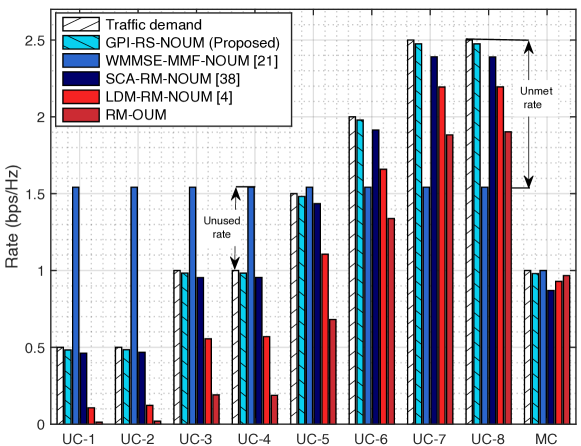
(a) Perfect CSIT

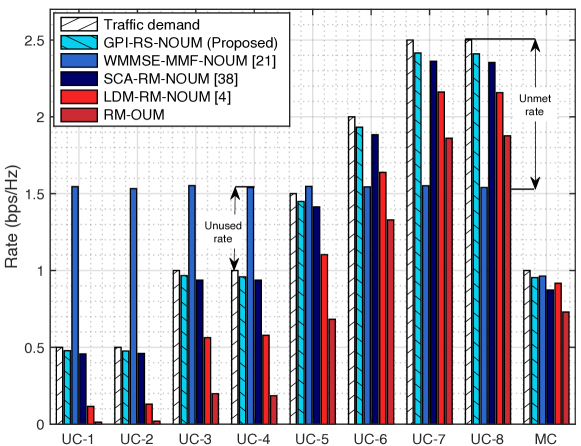
(b) Imperfect CSIT

Figure 2: Achievable rate comparison for each message. The unicast and multicast traffic demands are set to be $\mathbf{r}_{\sf target,uc}=[0.5,0.5,1,1,1.5,2,2.5,2.5]^{\sf{T}}$ bps/Hz and $R_{\sf target,mc}=1$ bps/Hz.

We compare the achievable rate of each scheme under both perfect and imperfect CSIT cases through Fig. 2(a) and Fig. 2(b). The leftmost white bar represents the traffic demand of each message, where the traffic demands of unicast and multicast messages are set to be $\mathbf{r}_{\sf target,uc}=[0.5,0.5,1,1,1.5,2,2.5,2.5]^{\sf{T}}$ bps/Hz and $R_{\sf target,mc}=1$ bps/Hz, respectively. As shown in the figures, the proposed GPI-RS-NOUM framework achieves superior performance over benchmark schemes in terms of traffic demand satisfaction, demonstrating substantial improvements regardless of CSI conditions. In particular, we observe that WMMSE-MMF-NOUM leads to pronounced unused or unmet unicast rates in both perfect and imperfect CSIT cases due to its oversight of non-uniform unicast demand distribution.

The considerable performance gap between the proposed scheme and LDM-RM-NOUM, illustrated in Fig. 2(a) and Fig. 2(b), stems from the pivotal role played by the common stream. To elaborate more in detail, we provide the rate portion comparison between GPI-RS-NOUM and LDM-RM-NOUM in Fig. 3. The blue, yellow, and orange bars in Fig. 3 denote the rate portion of common, multicast, and private streams, respectively. Since we aim to minimize the sum of disparity between traffic demands and actual offered rates, in LDM-RM-NOUM, the LEO satellite prioritizes fulfilling the traffic demands of users with higher unicast traffic demands. During this process, significant inter-user interference is induced on users with lower unicast traffic demands, exacerbating the rate-matching performance. Moreover, owing to inter-user interference among the users with high unicast traffic demands, it turns out that those are also not completely met. Additionally, interference from unicast messages to the multicast message leads to the disparity between the traffic demands and actual offered rates. The proposed GPI-RS-NOUM scheme utilizes a common stream decodable by all users not only for serving the multicast message but also for partially fulfilling unicast traffic demands, as depicted in Fig. 3. In other words, the proposed scheme allows the LEO satellite to flexibly adjust transmit power for common and private streams according to the traffic demands; the proposed GPI-RS-NOUM scheme, in turn, effectively reduces inter-user interference and interference from unicast messages to the multicast message, enabling it to uniformly satisfy the traffic demands of both unicast and multicast messages. Further, it is shown that the proposed scheme outperforms SCA-RM-NOUM in terms of satisfying traffic demands for all messages. This is because the proposed scheme expresses the first-order KKT condition of the reformulated problem into NEPv, achieving the best local optimal point via the GPI-based method. On the other hand, SCA-RM-NOUM combines SCA and MMSE methods, designing the RSMA precoder that is not optimal. Meanwhile, RM-OUM exhibits the worst performance due to inefficient resource utilization.

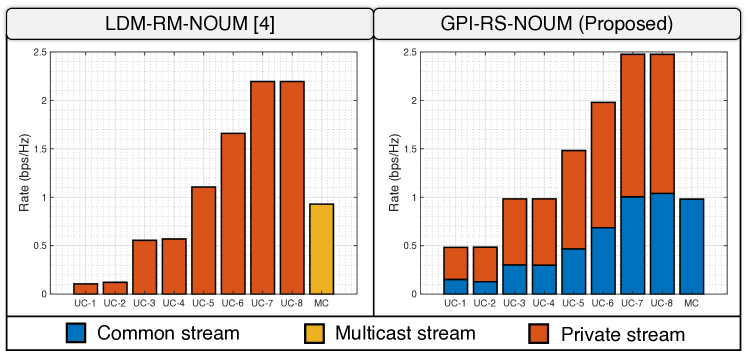
Figure 3: Rate portion comparison between GPI-RS-NOUM and LDM-RM-NOUM for each message under perfect CSIT. The unicast and multicast traffic demands are set to be $\mathbf{r}_{\sf target,uc}=[0.5,0.5,1,1,1.5,2,2.5,2.5]^{\sf{T}}$ and $R_{\sf target,mc}=1$ bps/Hz.

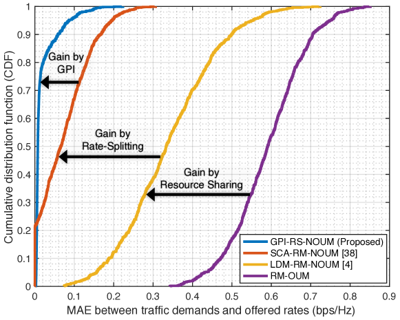
(a) Perfect CSIT

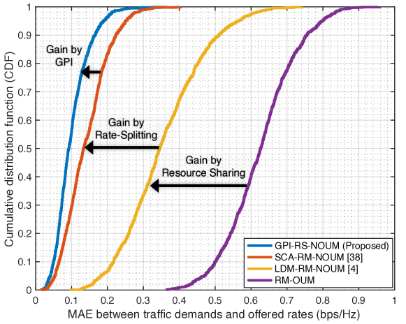
(b) Imperfect CSIT

Figure 4: Comparison of CDF per MAE between the traffic demands and offered rates. The unicast and multicast traffic demands are set as $\mathbf{r}_{\sf target,uc}=[0.5,0.5,1,1,1.5,2,2.5,2.5]^{\sf{T}}$ bps/Hz and $R_{\sf target,mc}=1$ bps/Hz.

Rate-matching error comparison

The rate-matching error is compared in Fig. 4(a) and Fig. 4(b) under $\mathbf{r}_{\sf target,uc}=[0.5,0.5,1,1,1.5,2,2.5,2.5]^{\sf{T}}$ bps/Hz and $R_{\sf target,mc}=1$ bps/Hz. The cumulative distribution function (CDF) is demonstrated under perfect and imperfect CSIT in Fig. 4(a) and Fig. 4(b), respectively. The x-axis presents the mean absolute error (MAE) between the traffic demands and offered rates, i.e.,

$$\frac{1}{K+1}\bigg{(}\sum_{j=1}^{K}{\left|R_{{\sf{target}},j}-R_{j}^{\sf{ins}}\right|}+{\left|R_{\sf{target,mc}}-C_{\sf{mc}}^{\sf{ins}}\right|}\bigg{)},$$ (61)

where lower levels indicate better performance. Overall, as depicted in Fig. 4(a) and Fig. 4(b), the proposed scheme exhibits the lowest MAE levels compared to the benchmark schemes regardless of the CSIT condition. To elaborate further, compared to SCA-RM-NOUM, our proposed scheme achieves a $95$-percentile MAE reduction of approximately $55.6$ and $24.7$ $\%$ under perfect and imperfect CSIT conditions, respectively. Compared to LDM-RM-NOUM, our scheme demonstrates a reduction of about $84.3$ and $66.6$ $\%$ under perfect and imperfect CSIT conditions, respectively. Additionally, compared to RM-OUM, our scheme exhibits reductions of approximately $88.4$ and $76.4$ $\%$ under perfect and imperfect CSIT conditions, respectively. Consequently, the superior performance of our proposed scheme demonstrates its capability to ensure stable traffic demand satisfaction for both unicast and multicast messages, regardless of the CSIT conditions and user locations.

Rate-matching error per multicast traffic demand

We depict the average value of MAE (AMAE) for $1,000$ channel realizations per different multicast traffic demands through Fig. 5. Herein, we assume that the LEO satellite is equipped with $36$ transmit antennas, arranged in a $6\times 6$ UPA configuration, and the unicast traffic demands are fixed to $\mathbf{r}_{\sf target,uc}=[0.5,0.5,1,1,1.5,2,2.5,2.5]^{\sf{T}}$ bps/Hz. In Fig. 5, the lower y-axis value indicates better performance. The solid line and dashed line represent the perfect and imperfect CSIT scenarios, respectively. Under both perfect and imperfect CSIT cases, the proposed GPI-RS-NOUM framework outperforms benchmark schemes in terms of AMAE regardless of the multicast traffic demand. In particular, even when a perfect CSIT is not available, the proposed scheme shows a better AMAE level compared to LDM-RM-NOUM and RM-OUM with a perfect CSIT, thanks to the common stream and efficient resource reuse. Moreover, when the multicast traffic demand exceeds $1.75$ bps/Hz, the proposed scheme with imperfect CSIT demonstrates superior AMAE performance compared to the SCA-RM-NOUM with perfect CSIT.

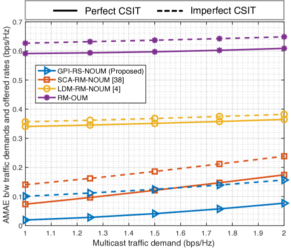
Figure 5: Comparison of AMAE per multicast traffic demand. The unicast traffic demands are set as $\mathbf{r}_{\sf target,uc}=[0.5,0.5,1,1,1.5,2,2.5,2.5]^{\sf{T}}$ bps/Hz.

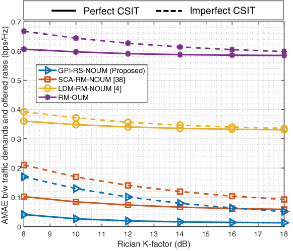
Figure 6: Comparison of AMAE per Rician K-factor. The unicast and multicast traffic demands are set as $\mathbf{r}_{\sf target,uc}=[0.5,0.5,1,1,1.5,2,2.5,2.5]^{\sf{T}}$ bps/Hz and $R_{\sf target,mc}=1$ bps/Hz.

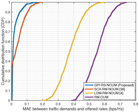
(a) Perfect CSIT with $N_{\sf{t}}=16$ (i.e., $N_{\sf{t}}^{x}=N_{\sf{t}}^{y}=4$)

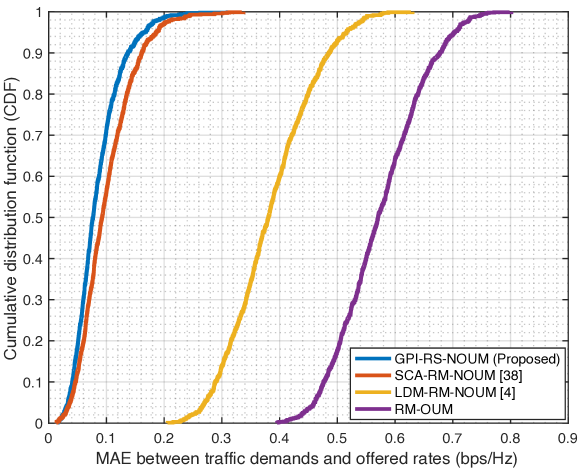
(b) Imperfect CSIT with $N_{\sf{t}}=16$ (i.e., $N_{\sf{t}}^{x}=N_{\sf{t}}^{y}=4$)

Figure 7: Comparison of CDF per MAE when the number of transmit antenna is set as $N_{\sf{t}}=16$. The unicast and multicast traffic demands are $\mathbf{r}_{\sf target,uc}=[0.5,0.5,0.5,1,1,1.5,2,2]^{\sf{T}}$ bps/Hz and $R_{\sf target,mc}=0.5$ bps/Hz.

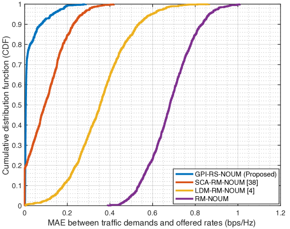
(a) Perfect CSIT with $N_{\sf{t}}=64$ (i.e., $N_{\sf{t}}^{x}=N_{\sf{t}}^{y}=8$)

(b) Imperfect CSIT with $N_{\sf{t}}=64$ (i.e., $N_{\sf{t}}^{x}=N_{\sf{t}}^{y}=8$)

Figure 8: Comparison of CDF per MAE when the number of transmit antenna is set as $N_{\sf{t}}=64$. The unicast and multicast traffic demands are $\mathbf{r}_{\sf target,uc}=[1,1,1.5,1.5,2,2,3,3]^{\sf{T}}$ bps/Hz and $R_{\sf target,mc}=1$ bps/Hz.

Rate-matching error per Rician K-factor

To shed light on the rate-matching error performance in comprehensive LEO SATCOM environments, we illustrate the AMAE per different Rician K-factor in Fig. 6. In Fig. 6, the lower value on the y-axis denotes superior performance, and the solid and dashed lines, respectively, illustrate the results under perfect and imperfect CSIT scenarios. The number of transmit antenna $N_{\sf{t}}$ is set to be $N_{\sf{t}}=36$ (i.e., $N_{\sf{t}}^{x}=N_{\sf{t}}^{y}=6$), and the unicast and multicast traffic demands are respectively configured as $\mathbf{r}_{\sf target,uc}=[0.5,0.5,1,1,1.5,2,2.5,2.5]^{\sf{T}}$ bps/Hz and $R_{\sf target,mc}=1$ bps/Hz. The results clearly show the superior performance of the proposed GPI-RS-NOUM framework in terms of AMAE, irrespective of the Rician K-factor, for both perfect and imperfect CSIT scenarios. This implies that the proposed scheme can reliably fulfill both unicast and multicast traffic demands, despite variations in the Rician K-factor due to elevation angle and scattering conditions of the target service area. Furthermore, it can be observed that as the Rician K-factor increases, the performance gap between perfect and imperfect CSIT cases diminishes. This is because, as the Rician K-factor increases, the channel relies more on the geometrical relation of satellite-to-users due to the increased strength of the LOS path compared to the non-LOS paths, tightening our upper bound for ergodic rate expressions.

Rate-matching error in different numbers of transmit antennas and various traffic demand distributions

To consider small- and large-scale antenna configurations, we conduct a numerical analysis under the scenarios with $N_{\sf{t}}=16$ (i.e., UPA with $4\times 4$ antennas) and $N_{\sf{t}}=64$ (i.e., UPA with $8\times 8$ antennas). Through Fig. 7(a) and Fig. 7(b), we first depict the CDF for MAE under perfect and imperfect CSIT cases when the number of transmit antennas $N_{\sf{t}}$ is set as $N_{\sf{t}}=16$. In such a setup, the unicast and multicast traffic demands are set to be $\mathbf{r}_{\sf{target,uc}}=[0.5,0.5,0.5,1,1,1.5,2,2]^{\sf{T}}$ bps/Hz and $R_{\sf{target,mc}}=0.5$ bps/Hz, respectively. As can be observed from the figures, the proposed GPI-RS-NOUM framework shows superior MAE performance compared to the benchmarks for both perfect and imperfect CSIT conditions.

Subsequently, the CDF for MAE with $N_{\sf{t}}=64$ under perfect and imperfect CSIT are illustrated in Fig. 8(a) and Fig. 8(b), respectively. The traffic demands of unicast and multicast messages are set to be $\mathbf{r}_{\sf{target,uc}}=[1,1,1.5,1.5,2,2,3,3]^{\sf{T}}$ bps/Hz and $R_{\sf{target,mc}}=1$ bps/Hz, respectively. From the simulations, we observe that the proposed scheme achieves a reduction of around $51$ and $32$ $\%$ in the $95$-percentile of MAE compared to SCA-RM-NOUM under perfect and imperfect CSIT, respectively. Compared to LDM-RM-NOUM, the proposed scheme exhibits a decrease of approximately $77.7$ and $61.6$ $\%$ under perfect and imperfect CSIT conditions. In addition, the proposed scheme shows a decrease of around $84.7$ and $74$ $\%$ compared to RM-OUM under perfect and imperfect CSIT conditions. These imply that the proposed GPI-RS-NOUM scheme stably satisfies the non-uniform unicast traffic demands and effectively provides the required multicast service, irrespective of the number of transmit antennas.

Convergence analysis

Fig. 9(a) and Fig. 9(b) illustrate the convergence behavior of the proposed GPI-RS-NOUM algorithm for random channel realizations under imperfect CSIT, where the user locations are randomly determined for each realization. For $N_{\sf{t}}^{x}=N_{\sf{t}}^{y}=8$, the unicast and multicast traffic demands are set to $\mathbf{r}_{\sf target,uc}=[1,1,1.5,1.5,2,2,3,3]^{\sf{T}}$ bps/Hz and $R_{\sf target,mc}=1$ bps/Hz, respectively. For $N_{\sf{t}}^{x}=N_{\sf{t}}^{y}=6$, the traffic demands are set to $\mathbf{r}_{\sf target,uc}=[0.5,0.5,1,1,1.5,2,2.5,2.5]^{\sf{T}}$ bps/Hz and $R_{\sf target,mc}=1$ bps/Hz. For $N_{\sf{t}}^{x}=N_{\sf{t}}^{y}=4$, they are $\mathbf{r}_{\sf target,uc}=[0.5,0.5,0.5,1,1,1.5,2,2]^{\sf{T}}$ bps/Hz and $R_{\sf target,mc}=0.5$ bps/Hz. It can be observed that the precoding vector $\bar{\mathbf{f}}$ converges after several iterations, while ${\mathbf{v}}$ converges even more rapidly. These results demonstrate that the convergence of the proposed GPI-RS-NOUM algorithm is well assured in various LEO SATCOM environments.

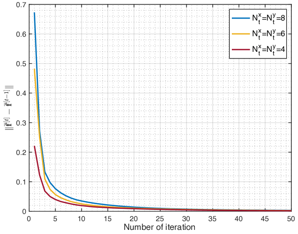
(a) Residual value of $\bar{\mathbf{f}}$

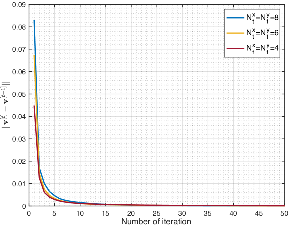
(b) Residual value of ${\mathbf{v}}$

Figure 9: Convergence behavior of the proposed GPI-RS-NOUM algorithm under imperfect CSIT.

V Conclusion and Future Directions

This paper has explored an RSMA-based RM framework for NOUM transmission in LEO SATCOM in the presence of imperfect CSIT. We have formulated the problem of minimizing the difference between the traffic demands and actual offered rates for both unicast and multicast messages. To address the challenges posed by the non-smoothness and non-convexity of the formulated problem, we have employed the LogSumExp technique to approximate the minimum common rate. Subsequently, we have reformulated the common rate portion as the ratio of the approximated function, transforming the problem into an unconstrained form. We have demonstrated that the first-order KKT condition of the reformulated problem is cast as an NEPv. To efficiently compute its principal eigenvector, the GPI-RS-NOUM algorithm has been introduced. Extensive numerical analysis in diverse LEO SATCOM environments has verified the superior performance of the proposed scheme in terms of traffic demand satisfaction compared to the benchmarks.

For future directions, it is promising to consider multiple receive antennas at the receiver to further improve spectral efficiency under severe path attenuation of LEO SATCOM while minimizing the increased cost and energy consumption of mobile devices. This can be accomplished by introducing analog hardware, such as controllable phase shifters, or by optimizing the selection of antennas connected to the single RF chain based on the receive antenna selection technique [39, 40]. Additionally, adapting machine learning approaches, such as deep learning and deep reinforcement learning, in RSMA-based rate matching precoder design is promising. Further reducing the computational complexity to achieve more practical and efficient real-world implementations, considering the constraints on onboard resources and computation in LEO satellites, is also of interest.

VI Appendix A: Proof of Lemma 1

The first-order KKT condition of the problem (38) to $\bar{\mathbf{f}}$ is expanded as (VI) at the top of the next page since we have

$$\frac{\partial}{\partial{\bar{\mathbf{f}}}}\left\{\log_{2}\left(\frac{\bar{\mathbf{f}}^{\sf{H}}\mathbf{A}^{\sf{p}}_{k}\bar{\mathbf{f}}}{\bar{\mathbf{f}}^{\sf{H}}\mathbf{B}^{\sf{p}}_{k}\bar{\mathbf{f}}}\right)\right\}=\frac{2}{\ln 2}\left(\frac{\mathbf{A}^{\sf{p}}_{k}}{\bar{\mathbf{f}}^{\sf{H}}\mathbf{A}^{\sf{p}}_{k}\bar{\mathbf{f}}}-\frac{\mathbf{B}^{\sf{p}}_{k}}{\bar{\mathbf{f}}^{\sf{H}}\mathbf{B}^{\sf{p}}_{k}\bar{\mathbf{f}}}\right)\bar{\mathbf{f}}$$ (62)

and

$$\frac{\partial}{\partial{\bar{\mathbf{f}}}}\left\{\log\left(\frac{1}{K}\sum_{i=1}^{K}\exp\left(-\frac{1}{\alpha}\log_{2}\left(\frac{\bar{\mathbf{f}}^{\sf{H}}\mathbf{A}_{i}^{\sf{c}}\bar{\mathbf{f}}}{\bar{\mathbf{f}}^{\sf{H}}\mathbf{B}_{i}^{\sf{c}}\bar{\mathbf{f}}}\right)\right)\right)^{-\alpha}\right\}\!=\!\frac{2}{\ln{2}}\times$$

$$\sum_{i=1}^{K}\left({\frac{\exp\left(-\frac{1}{\alpha}\log_{2}\left(\frac{\bar{\mathbf{f}}^{\sf{H}}\mathbf{A}_{i}^{\sf{c}}\bar{\mathbf{f}}}{\bar{\mathbf{f}}^{\sf{H}}\mathbf{B}_{i}^{\sf{c}}\bar{\mathbf{f}}}\right)\right)}{\sum_{\ell=1}^{K}{\exp\left(-\frac{1}{\alpha}\log_{2}\left(\frac{\bar{\mathbf{f}}^{\sf{H}}\mathbf{A}_{\ell}^{\sf{c}}\bar{\mathbf{f}}}{\bar{\mathbf{f}}^{\sf{H}}\mathbf{B}_{\ell}^{\sf{c}}\bar{\mathbf{f}}}\right)\right)}}}\left(\frac{{\mathbf{A}_{i}^{\sf{c}}}}{\bar{\mathbf{f}}^{\sf{H}}{\mathbf{A}_{i}^{\sf{c}}}{\bar{\mathbf{f}}}}-\frac{{\mathbf{B}_{i}^{\sf{c}}}}{\bar{\mathbf{f}}^{\sf{H}}{\mathbf{B}_{i}^{\sf{c}}}{\bar{\mathbf{f}}}}\right)\right)$$

$$=\frac{2}{\ln{2}}\left(\mathbf{L}_{\sf{A}}(\bar{\mathbf{f}})-\mathbf{L}_{\sf{B}}(\bar{\mathbf{f}})\right){\bar{\mathbf{f}}}.$$ (63)

Subsequently, defining $\mathbf{A}(\bar{\mathbf{f}},\mathbf{v})$, $\mathbf{B}(\bar{\mathbf{f}},\mathbf{v})$, $\lambda(\bar{\mathbf{f}},\mathbf{v})$, $\lambda_{\sf{num}}(\bar{\mathbf{f}},\mathbf{v})$, and $\lambda_{\sf{den}}(\bar{\mathbf{f}},\mathbf{v})$ as (1), (1), (1), (1), and (47), respectively, the equation (VI) is rearranged as

$$\frac{\partial{f(\bar{\mathbf{f}},\mathbf{v})}}{\partial{\bar{\mathbf{f}}}} =\sum_{j=1}^{K}\Bigg{[}-R_{{\sf{target}},j}\left\{\frac{\mathbf{A}^{\sf{p}}_{j}\bar{\mathbf{f}}}{\bar{\mathbf{f}}^{\sf{H}}\mathbf{A}^{\sf{p}}_{j}\bar{\mathbf{f}}}-\frac{\mathbf{B}^{\sf{p}}_{j}\bar{\mathbf{f}}}{\bar{\mathbf{f}}^{\sf{H}}\mathbf{B}^{\sf{p}}_{j}\bar{\mathbf{f}}}\right\}-R_{{\sf{target}},j}\frac{\mathbf{v}^{\sf{H}}\mathbf{E}_{j}\mathbf{v}}{\mathbf{v}^{\sf{H}}\mathbf{v}}\left\{\mathbf{L}_{\sf{A}}(\bar{\mathbf{f}})-\mathbf{L}_{\sf{B}}(\bar{\mathbf{f}})\right\}+\log_{2}\left(\frac{\bar{\mathbf{f}}^{\sf{H}}\mathbf{A}_{j}^{\sf{p}}\bar{\mathbf{f}}}{\bar{\mathbf{f}}^{\sf{H}}\mathbf{B}_{j}^{\sf{p}}\bar{\mathbf{f}}}\right)\left\{\frac{\mathbf{A}^{\sf{p}}_{j}\bar{\mathbf{f}}}{\bar{\mathbf{f}}^{\sf{H}}\mathbf{A}^{\sf{p}}_{j}\bar{\mathbf{f}}}-\frac{\mathbf{B}^{\sf{p}}_{j}\bar{\mathbf{f}}}{\bar{\mathbf{f}}^{\sf{H}}\mathbf{B}^{\sf{p}}_{j}\bar{\mathbf{f}}}\right\}$$

$$+\left(\frac{\mathbf{v}^{\sf{H}}\mathbf{E}_{j}\mathbf{v}}{\mathbf{v}^{\sf{H}}\mathbf{v}}\right)^{2}\log\left(\frac{1}{K}\sum_{i=1}^{K}\exp\left(-\frac{1}{\alpha}\log_{2}\left(\frac{\bar{\mathbf{f}}^{\sf{H}}\mathbf{A}_{i}^{\sf{c}}\bar{\mathbf{f}}}{\bar{\mathbf{f}}^{\sf{H}}\mathbf{B}_{i}^{\sf{c}}\bar{\mathbf{f}}}\right)\right)\right)^{-\alpha}\!\!\!\!\!\!\left\{\mathbf{L}_{\sf{A}}(\bar{\mathbf{f}})-\mathbf{L}_{\sf{B}}(\bar{\mathbf{f}})\right\}+\frac{\mathbf{v}^{\sf{H}}\mathbf{E}_{j}\mathbf{v}}{\mathbf{v}^{\sf{H}}\mathbf{v}}\log_{2}\left(\frac{\bar{\mathbf{f}}^{\sf{H}}\mathbf{A}_{j}^{\sf{p}}\bar{\mathbf{f}}}{\bar{\mathbf{f}}^{\sf{H}}\mathbf{B}_{j}^{\sf{p}}\bar{\mathbf{f}}}\right)\left\{\mathbf{L}_{\sf{A}}(\bar{\mathbf{f}})-\mathbf{L}_{\sf{B}}(\bar{\mathbf{f}})\right\}$$

$$+\frac{\mathbf{v}^{\sf{H}}\mathbf{E}_{j}\mathbf{v}}{\mathbf{v}^{\sf{H}}\mathbf{v}}\log\left(\frac{1}{K}\sum_{i=1}^{K}\exp\left(-\frac{1}{\alpha}\log_{2}\left(\frac{\bar{\mathbf{f}}^{\sf{H}}\mathbf{A}_{i}^{\sf{c}}\bar{\mathbf{f}}}{\bar{\mathbf{f}}^{\sf{H}}\mathbf{B}_{i}^{\sf{c}}\bar{\mathbf{f}}}\right)\right)\right)^{-\alpha}\!\!\!\!\!\cdot\left\{\frac{\mathbf{A}^{\sf{p}}_{j}\bar{\mathbf{f}}}{\bar{\mathbf{f}}^{\sf{H}}\mathbf{A}^{\sf{p}}_{j}\bar{\mathbf{f}}}-\frac{\mathbf{B}^{\sf{p}}_{j}\bar{\mathbf{f}}}{\bar{\mathbf{f}}^{\sf{H}}\mathbf{B}^{\sf{p}}_{j}\bar{\mathbf{f}}}\right\}\Bigg{]}+\eta_{\sf{mc}}\Bigg{[}-R_{{\sf{target,mc}}}\frac{\mathbf{v}^{\sf{H}}\mathbf{E}_{K+1}\mathbf{v}}{\mathbf{v}^{\sf{H}}\mathbf{v}}\left\{\mathbf{L}_{\sf{A}}(\bar{\mathbf{f}})-\mathbf{L}_{\sf{B}}(\bar{\mathbf{f}})\right\}$$

$$+\left(\frac{\mathbf{v}^{\sf{H}}\mathbf{E}_{K+1}\mathbf{v}}{\mathbf{v}^{\sf{H}}\mathbf{v}}\right)^{2}\log\left(\frac{1}{K}\sum_{i=1}^{K}\exp\left(-\frac{1}{\alpha}\log_{2}\left(\frac{\bar{\mathbf{f}}^{\sf{H}}\mathbf{A}_{i}^{\sf{c}}\bar{\mathbf{f}}}{\bar{\mathbf{f}}^{\sf{H}}\mathbf{B}_{i}^{\sf{c}}\bar{\mathbf{f}}}\right)\right)\right)^{-\alpha}\!\!\!\!\!\!\left\{\mathbf{L}_{\sf{A}}(\bar{\mathbf{f}})-\mathbf{L}_{\sf{B}}(\bar{\mathbf{f}})\right\}\Bigg{]}=\mathbf{0}$$ (64)

 

$$\mathbf{A}(\bar{\mathbf{f}},\mathbf{v})\bar{\mathbf{f}}=\lambda(\bar{\mathbf{f}},\mathbf{v})\mathbf{B}(\bar{\mathbf{f}},\mathbf{v})\bar{\mathbf{f}}.$$ (65)

We note that since $\mathbf{A}(\bar{\mathbf{f}},\mathbf{v})$ and $\mathbf{B}(\bar{\mathbf{f}},\mathbf{v})$ are expressed as the summation of positive definite (PD) matrices and positive semi-definite (PSD) matrices, both $\mathbf{A}(\bar{\mathbf{f}},\mathbf{v})$ and $\mathbf{B}(\bar{\mathbf{f}},\mathbf{v})$ are PD matrices; thus, $\mathbf{A}(\bar{\mathbf{f}},\mathbf{v})$ and $\mathbf{B}(\bar{\mathbf{f}},\mathbf{v})$ are invertible matrices. Thanks to this feature, (65) can be rewritten as

$${\mathbf{B}(\bar{\mathbf{f}},\mathbf{v})}^{-1}{\mathbf{A}(\bar{\mathbf{f}},\mathbf{v})}\bar{\mathbf{f}}=\lambda(\bar{\mathbf{f}},\mathbf{v})\bar{\mathbf{f}},$$ (66)

and this completes the proof.

VII Appendix B: Proof of Lemma 2

The first-order KKT condition of the problem (38) to ${\mathbf{v}}$ is expanded as (VII) at the top of this page since we have

$$\frac{\partial}{\partial{{\mathbf{v}}}}\left\{\frac{\mathbf{v}^{\sf{H}}\mathbf{E}_{k}\mathbf{v}}{\mathbf{v}^{\sf{H}}\mathbf{v}}\right\} =\frac{2\mathbf{E}_{k}\mathbf{v}}{\mathbf{v}^{\sf{H}}\mathbf{v}}-\frac{2\mathbf{v}^{\sf{H}}\mathbf{E}_{k}\mathbf{v}}{(\mathbf{v}^{\sf{H}}\mathbf{v})^{2}}\mathbf{v}$$

$$=2\left(\frac{\mathbf{E}_{k}}{\mathbf{v}^{\sf{H}}\mathbf{v}}-\frac{\mathbf{v}^{\sf{H}}\mathbf{E}_{k}\mathbf{v}}{(\mathbf{v}^{\sf{H}}\mathbf{v})^{2}}\mathbf{I}\right)\mathbf{v}.$$ (67)

Subsequently, defining $\mathbf{D}(\bar{\mathbf{f}},\mathbf{v})$, $\mathbf{E}(\bar{\mathbf{f}},\mathbf{v})$, $\lambda(\bar{\mathbf{f}},\mathbf{v})$, $\lambda_{\sf{num}}(\bar{\mathbf{f}},\mathbf{v})$, and $\lambda_{\sf{den}}(\bar{\mathbf{f}},\mathbf{v})$ as (2), (2), (1), (1), and (47), respectively, the equation (VII) is rearranged as

$$\frac{\partial{f(\bar{\mathbf{f}},\mathbf{v})}}{\partial{{\mathbf{v}}}} =\sum_{j=1}^{K}\Bigg{[}-R_{{\sf{target}},j}\left\{\frac{\mathbf{E}_{j}\mathbf{v}}{\mathbf{v}^{\sf{H}}\mathbf{v}}-\frac{\mathbf{v}^{\sf{H}}\mathbf{E}_{j}\mathbf{v}}{(\mathbf{v}^{\sf{H}}\mathbf{v})^{2}}\mathbf{v}\right\}+\log\left(\frac{1}{K}\sum_{i=1}^{K}\exp\left(-\frac{1}{\alpha}\log_{2}\left(\frac{\bar{\mathbf{f}}^{\sf{H}}\mathbf{A}_{i}^{\sf{c}}\bar{\mathbf{f}}}{\bar{\mathbf{f}}^{\sf{H}}\mathbf{B}_{i}^{\sf{c}}\bar{\mathbf{f}}}\right)\right)\right)^{-\alpha}\!\!\!\!\!\!\cdot\frac{\mathbf{v}^{\sf{H}}\mathbf{E}_{j}\mathbf{v}}{\mathbf{v}^{\sf{H}}\mathbf{v}}\left\{\frac{\mathbf{E}_{j}\mathbf{v}}{\mathbf{v}^{\sf{H}}\mathbf{v}}-\frac{\mathbf{v}^{\sf{H}}\mathbf{E}_{j}\mathbf{v}}{(\mathbf{v}^{\sf{H}}\mathbf{v})^{2}}\mathbf{v}\right\}$$

$$+\log_{2}\left(\frac{\bar{\mathbf{f}}^{\sf{H}}\mathbf{A}_{j}^{\sf{p}}\bar{\mathbf{f}}}{\bar{\mathbf{f}}^{\sf{H}}\mathbf{B}_{j}^{\sf{p}}\bar{\mathbf{f}}}\right)\left\{\frac{\mathbf{E}_{j}\mathbf{v}}{\mathbf{v}^{\sf{H}}\mathbf{v}}-\frac{\mathbf{v}^{\sf{H}}\mathbf{E}_{j}\mathbf{v}}{(\mathbf{v}^{\sf{H}}\mathbf{v})^{2}}\mathbf{v}\right\}\Bigg{]}+\eta_{\sf{mc}}\Bigg{[}-R_{\sf{target,mc}}\left\{\frac{\mathbf{E}_{K+1}\mathbf{v}}{\mathbf{v}^{\sf{H}}\mathbf{v}}-\frac{\mathbf{v}^{\sf{H}}\mathbf{E}_{K+1}\mathbf{v}}{(\mathbf{v}^{\sf{H}}\mathbf{v})^{2}}\mathbf{v}\right\}$$

$$+\log\left(\frac{1}{K}\sum_{i=1}^{K}\exp\left(-\frac{1}{\alpha}\log_{2}\left(\frac{\bar{\mathbf{f}}^{\sf{H}}\mathbf{A}_{i}^{\sf{c}}\bar{\mathbf{f}}}{\bar{\mathbf{f}}^{\sf{H}}\mathbf{B}_{i}^{\sf{c}}\bar{\mathbf{f}}}\right)\right)\right)^{-\alpha}\!\!\!\!\!\!\cdot\frac{\mathbf{v}^{\sf{H}}\mathbf{E}_{K+1}\mathbf{v}}{\mathbf{v}^{\sf{H}}\mathbf{v}}\left\{\frac{\mathbf{E}_{K+1}\mathbf{v}}{\mathbf{v}^{\sf{H}}\mathbf{v}}-\frac{\mathbf{v}^{\sf{H}}\mathbf{E}_{K+1}\mathbf{v}}{(\mathbf{v}^{\sf{H}}\mathbf{v})^{2}}\mathbf{v}\right\}\Bigg{]}=\mathbf{0}$$ (68)

 

$$\mathbf{D}(\bar{\mathbf{f}},\mathbf{v}){\mathbf{v}}=\lambda(\bar{\mathbf{f}},\mathbf{v})\mathbf{E}(\bar{\mathbf{f}},\mathbf{v}){\mathbf{v}}.$$ (69)

We note that since $\mathbf{D}(\bar{\mathbf{f}},\mathbf{v})$ and $\mathbf{E}(\bar{\mathbf{f}},\mathbf{v})$ are expressed as the summation of PD matrices and PSD matrices, both $\mathbf{D}(\bar{\mathbf{f}},\mathbf{v})$ and $\mathbf{E}(\bar{\mathbf{f}},\mathbf{v})$ are PD matrices; thus, $\mathbf{D}(\bar{\mathbf{f}},\mathbf{v})$ and $\mathbf{E}(\bar{\mathbf{f}},\mathbf{v})$ are invertible matrices. Thanks to this feature, (65) can be rewritten as

$${\mathbf{E}(\bar{\mathbf{f}},\mathbf{v})}^{-1}{\mathbf{D}(\bar{\mathbf{f}},\mathbf{v})}{\mathbf{v}}=\lambda(\bar{\mathbf{f}},\mathbf{v}){\mathbf{v}},$$ (70)

and this completes the proof.

References

• [1] Y. Zhong, X. Ge, H. H. Yang, T. Han, and Q. Li, “Traffic matching in 5G ultra-dense networks,” IEEE Commun. Mag., vol. 56, no. 8, pp. 100–105, 2018.
• [2] A. I. Perez-Neira, M. A. Vazquez, M. B. Shankar, S. Maleki, and S. Chatzinotas, “Signal processing for high-throughput satellites: Challenges in new interference-limited scenarios,” IEEE Signal Process. Mag., vol. 36, no. 4, pp. 112–131, 2019.
• [3] Y. Kawamoto, Z. M. Fadlullah, H. Nishiyama, N. Kato, and M. Toyoshima, “Prospects and challenges of context-aware multimedia content delivery in cooperative satellite and terrestrial networks,” IEEE Commun. Mag., vol. 52, no. 6, pp. 55–61, 2014.
• [4] D. Kim, F. Khan, C. V. Rensburg, Z. Pi, and S. Yoon, “Superposition of broadcast and unicast in wireless cellular systems,” IEEE Commun. Mag., vol. 46, no. 7, pp. 110–117, 2008.
• [5] D. Peng, S. Domouchtsidis, S. Chatzinotas, Y. Li, and B. Ottersten, “Non-orthogonal multicast and unicast robust beamforming in integrated terrestrial-satellite networks,” in Proc. IEEE Glob. Commun. Conf. (GLOBECOM), 2022, pp. 2044–2049.
• [6] M. Á. Vázquez, A. Perez-Neira, D. Christopoulos, S. Chatzinotas, B. Ottersten, P.-D. Arapoglou, A. Ginesi, and G. Taricco, “Precoding in multibeam satellite communications: Present and future challenges,” IEEE Wireless Commun., vol. 23, no. 6, pp. 88–95, 2016.
• [7] L. You, K.-X. Li, J. Wang, X. Gao, X.-G. Xia, and B. Ottersten, “Massive MIMO transmission for LEO satellite communications,” IEEE J. Sel. Areas Commun., vol. 38, no. 8, pp. 1851–1865, 2020.
• [8] Y. Mao, B. Clerckx, and V. O. Li, “Rate-splitting multiple access for downlink communication systems: Bridging, generalizing, and outperforming SDMA and NOMA,” EURASIP J. Wirel. Commun. Netw., vol. 2018, no. 1, pp. 1–54, 2018.
• [9] B. Clerckx, H. Joudeh, C. Hao, M. Dai, and B. Rassouli, “Rate splitting for MIMO wireless networks: A promising PHY-layer strategy for LTE evolution,” IEEE Commun. Mag., vol. 54, no. 5, pp. 98–105, 2016.
• [10] Y. Mao, B. Clerckx, and V. O. Li, “Energy efficiency of rate-splitting multiple access, and performance benefits over SDMA and NOMA,” in Proc. IEEE 15th Int. Symp. Wireless Commun. Sys., 2018, pp. 1–5.
• [11] J. Park, B. Lee, J. Choi, H. Lee, N. Lee, S.-H. Park, K.-J. Lee, J. Choi, S. H. Chae, S.-W. Jeon, K. S. Kwak, B. Clerckx, and W. Shin, “Rate-splitting multiple access for 6G networks: Ten promising scenarios and applications,” IEEE Network, vol. 38, no. 3, pp. 128–136, 2024.
• [12] B. Clerckx, Y. Mao, R. Schober, and H. V. Poor, “Rate-splitting unifying SDMA, OMA, NOMA, and multicasting in MISO broadcast channel: A simple two-user rate analysis,” IEEE Wireless Commun. Lett., vol. 9, no. 3, pp. 349–353, 2019.
• [13] L. Yin and B. Clerckx, “Rate-splitting multiple access for multibeam satellite communications,” in Proc. IEEE Int. Conf. Commun. Workshops (ICC Workshops), 2020, pp. 1–6.
• [14] L. Yin and B. Clerckx, “Rate-splitting multiple access for multigroup multicast and multibeam satellite systems,” IEEE Trans. Commun., vol. 69, no. 2, pp. 976–990, 2020.
• [15] L. Yin, O. Dizdar, and B. Clerckx, “Rate-splitting multiple access for multigroup multicast cellular and satellite communications: PHY layer design and link-level simulations,” in Proc. IEEE Int. Conf. Commun. Workshops (ICC Workshops), 2021, pp. 1–6.
• [16] Z. W. Si, L. Yin, and B. Clerckx, “Rate-splitting multiple access for multigateway multibeam satellite systems with feeder link interference,” IEEE Trans. Commun., vol. 70, no. 3, pp. 2147–2162, 2022.
• [17] W. U. Khan, Z. Ali, E. Lagunas, A. Mahmood, M. Asif, A. Ihsan, S. Chatzinotas, B. Ottersten, and O. A. Dobre, “Rate splitting multiple access for next generation cognitive radio enabled LEO satellite networks,” IEEE Trans. Wireless Commun., vol. 22, no. 11, pp. 8423–8435, 2023.
• [18] Y. Xu, L. Yin, Y. Mao, W. Shin, and B. Clerckx, “Distributed rate-splitting multiple access for multilayer satellite communications,” IEEE Trans. Commun., 2024.
• [19] Y. Mao, B. Clerckx, and V. O. Li, “Rate-splitting for multi-antenna non-orthogonal unicast and multicast transmission: Spectral and energy efficiency analysis,” IEEE Trans. Commun., vol. 67, no. 12, pp. 8754–8770, 2019.
• [20] Z. Li, S. Wang, S. Han, and C. Li, “Non-orthogonal broadcast and unicast joint transmission for multibeam satellite system,” IEEE Trans. Broadcast., vol. 69, no. 3, pp. 647–660, 2023.
• [21] Z. Li, S. Han, L. Xiao, and M. Peng, “Cooperative non-orthogonal broadcast and unicast transmission for integrated satellite-terrestrial network,” IEEE Trans. Broadcast., 2023.
• [22] S. Han, Z. Li, Q. Xue, W. Meng, and C. Li, “Joint broadcast and unicast transmission based on RSMA and spectrum sharing for integrated satellite-terrestrial network,” IEEE Trans. Cogn. Commun. Netw., vol. 10, no. 3, pp. 1090–1103, 2024.
• [23] J. Lizarraga, P. Angeletti, N. Alagha, and M. Aloisio, “Flexibility performance in advanced Ka-band multibeam satellites,” in Proc. IEEE Int. Vacuum Electron. Conf. (IVEC), 2014, pp. 45–46.
• [24] “3rd generation partnership project; Technical specification group radio access network; Study on new radio (NR) to support non-terrestrial networks (Release 15),” Tech. Rep. 3GPP TR 38.811 V15.0.0, Jun. 2018.
• [25] B. R. Vojcic, R. L. Pickholtz, and L. B. Milstein, “Performance of DS-CDMA with imperfect power control operating over a low earth orbiting satellite link,” IEEE J. Sel. Areas Commun., vol. 12, no. 4, pp. 560–567, 1994.
• [26] W. Jiang and H. D. Schotten, “Initial beamforming for millimeter-wave and terahertz communications in 6G mobile systems,” in Proc. IEEE Wireless Commun. Netw. Conf. (WCNC), 2022, pp. 2613–2618.
• [27] K.-X. Li, L. You, J. Wang, X. Gao, C. G. Tsinos, S. Chatzinotas, and B. Ottersten, “Downlink transmit design for massive MIMO LEO satellite communications,” IEEE Trans. Commun., vol. 70, no. 2, pp. 1014–1028, 2021.
• [28] L. You, X. Qiang, K.-X. Li, C. G. Tsinos, W. Wang, X. Gao, and B. Ottersten, “Hybrid analog/digital precoding for downlink massive MIMO LEO satellite communications,” IEEE Trans. Wireless Commun., vol. 21, no. 8, pp. 5962–5976, 2022.
• [29] L. You, X. Qiang, C. G. Tsinos, F. Liu, W. Wang, X. Gao, and B. Ottersten, “Beam squint-aware integrated sensing and communications for hybrid massive MIMO LEO satellite systems,” IEEE J. Sel. Areas Commun., vol. 40, no. 10, pp. 2994–3009, 2022.
• [30] M. Röper, B. Matthiesen, D. Wübben, P. Popovski, and A. Dekorsy, “Beamspace MIMO for satellite swarms,” in Proc. IEEE Wireless Commun. Netw. Conf. (WCNC), 2022, pp. 1307–1312.
• [31] C. Shen and H. Li, “On the dual formulation of boosting algorithms,” IEEE Trans. Pattern Anal. Mach. Intell., vol. 32, no. 12, pp. 2216–2231, 2010.
• [32] Y. Cai, L.-H. Zhang, Z. Bai, and R.-C. Li, “On an eigenvector-dependent nonlinear eigenvalue problem,” SIAM J. Matrix Anal. Appl., vol. 39, no. 3, pp. 1360–1382, 2018.
• [33] J. Choi, N. Lee, S.-N. Hong, and G. Caire, “Joint user selection, power allocation, and precoding design with imperfect CSIT for multi-cell MU-MIMO downlink systems,” IEEE Trans. Wireless Commun., vol. 19, no. 1, pp. 162–176, 2019.
• [34] J. Park, J. Choi, N. Lee, W. Shin, and H. V. Poor, “Rate-splitting multiple access for downlink MIMO: A generalized power iteration approach,” IEEE Trans. Wireless Commun., vol. 22, no. 3, pp. 1588–1603, 2022.
• [35] S. Park, J. Choi, J. Park, W. Shin, and B. Clerckx, “Rate-splitting multiple access for quantized multiuser MIMO communications,” IEEE Trans. Wireless Commun., vol. 22, no. 11, pp. 7696–7711, 2023.
• [36] D. Kim, W. Shin, J. Park, and D. K. Kim, “Distributed precoding for satellite-terrestrial integrated networks without sharing CSIT: A rate-splitting approach,” arXiv preprint arXiv:2309.06325, 2023.
• [37] D. Kim, J. Choi, J. Park, and D. K. Kim, “Max–min fairness beamforming with rate-splitting multiple access: Optimization without a toolbox,” IEEE Wireless Commun. Lett., vol. 12, no. 2, pp. 232–236, 2023.
• [38] H. Cui, L. Zhu, Z. Xiao, B. Clerckx, and R. Zhang, “Energy-efficient RSMA for multigroup multicast and multibeam satellite communications,” IEEE Wireless Commun. Lett., vol. 12, no. 5, pp. 838–842, 2023.
• [39] T. Gong, N. Shlezinger, S. S. Ioushua, M. Namer, Z. Yang, and Y. C. Eldar, “RF chain reduction for MIMO systems: A hardware prototype,” IEEE Syst. J., vol. 14, no. 4, pp. 5296–5307, 2020.
• [40] M. Toka, M. Vaezi, and W. Shin, “Outage analysis of alamouti-NOMA scheme for hybrid satellite-terrestrial relay networks,” IEEE Internet Things J., vol. 10, no. 6, pp. 5293–5303, 2022.