Back-Projection Diffusion: Solving the Wideband Inverse Scattering Problem with Diffusion Models

Abstract

We present Wideband back-projection diffusion, an end-to-end probabilistic framework for approximating the posterior distribution induced by the inverse scattering map from wideband scattering data. This framework leverages conditional diffusion models coupled with the underlying physics of wave-propagation and symmetries in the problem, to produce highly accurate reconstructions. The framework introduces a factorization of the score function into a physics-based latent representation inspired by the filtered back-propagation formula and a conditional score function conditioned on this latent representation. These two steps are also constrained to obey symmetries in the formulation while being amenable to compression by imposing the rank structure found in the filtered back-projection formula. As a result, empirically, our framework is able to provide sharp reconstructions effortlessly, even recovering sub-Nyquist features in the multiple-scattering regime. It has low-sample and computational complexity, its number of parameters scales sub-linearly with the target resolution, and it has stable training dynamics.

1 Introduction

In this paper we study the problem of high-resolution reconstruction of scatterers arising from wave-based inverse problems [1, 2, 3]. Wave-based inverse problems aim to reconstruct the properties of an unknown medium by probing it with impinging waves and measuring the medium impulse response, in the form of scattered waves, at the boundary. This task naturally arises in many scientific applications: e.g. biomedical imaging [4], synthetic aperture radar [5], non-destructive testing [6], and geophysics [7].

Historically, the development of algorithmic pipelines for wave-based inverse problems has been hampered by three main issues. First, the diffraction limit [8, 9] limits the maximum resolution that a reconstruction can have. Following the Rayleigh criterion [10], one typically increases the resolution by increasing the frequency of the probing wave. However, this can sometimes be infeasible in practice, especially when data at high-frequency is not readily available. Second, the numerical problem lacks stability of the reconstruction [11]. Even though the problem is well-posed and stable at the continuum level, it becomes increasingly ill-posed in the finite-data regime. For classical methods based on PDE-constrained optimization, this translates into a myriad of spurious local minima [12], whereas in the case of ML-based methods, it translates to highly unstable training stages [13]. Third, the algorithmic pipeline of the inversion incurs a high computational cost. As the resolution increases to capture fine-grained details, the computational complexity of state-of-the-art methods typically increases super-linearly with respect to the number of degrees of freedom. [14, 15].

To bypass these issues, many methods have been proposed throughout the years, which we review in Section 1.2.1. Such techniques can be broadly categorized in two main groups: analytical techniques, which rely on asymptotic expansion coupled with painstakingly analysis of the mathematical properties of the operators [16], and optimization-based techniques in which a data misfit loss is minimized using gradient based methods with either geometrical [17] or PDE constraints [18, 19]. In general, there is a trade-off between computational cost and the quality of the reconstruction, and depending on the computational and time constraints of the downstream applications, often the PDE-constrained optimization techniques are the preferred methodology. Even though recent advances have been strikingly successful at accelerating the solution to the associated PDE [20, 14, 21, 22, 23], the overall algorithmic pipelines remain prohibitively expensive.

In this context, one alluring alternative is to reconstruct the quantities of interest directly from the scattered data, which amounts to parametrizing and finding the underlying non-linear inverse map. The advent of modern ML tools has spurred the development of several ML-based models seeking to approximate such a map. Such approaches, which we review in Section 1.2.2, usually rely on wideband data [13, 24], which has proven crucial to obtain high-resolution reconstructions, and on bespoke architectures [25, 26, 27] to avoid the pitfalls [28] of dealing with highly oscillatory data.

Unfortunately, approximating this map prototypically exhibits three challenges commonly encountered in scientific ML (SciML). First: obtaining the training data in this setting – whether synthetically or experimentally – comes at considerable expense, which bottlenecks the size of the models that can be trained to satisfy the stringent accuracy requirements. This necessitates the use of highly tailored architectures. Second: wave scattering involves non-smooth data that are recordings of highly oscillatory, broadband, scattered waveforms. These highly oscillatory (i.e. high-frequency) signals are known to greatly hamper the training dynamics of many machine learning algorithms [28] and thus require tailored strategies to mitigate their effect. Third, current downstream applications often require quantification of the uncertainty on the reconstruction, which necessitates to learn the distribution of all possible reconstructions for a given input. This usually involves stochastic methods that require the repeated application of the reconstruction, and thus rapidly increases the overall cost.

While, many recently proposed ML-based methodologies [24, 27, 26, 13, 29, 30] have been able to bypass the first two challenges, they are usually deterministic, so they do not provide any quantification of uncertainty natively.

Quantifying uncertainty in the reconstruction has a long story dating back to the Bayesian formulation of the inverse problem championed by Tarantola in the 80’s [2, 31]. In a nutshell, we seek to obtain the distribution of possible reconstructions conditioned on the input data, instead of one particular reconstruction. Unfortunately, computing such distribution becomes computationally intractable as the dimension of the problem grows.

However, recent advances in generative models have shown that it is possible to approximate high-dimensional distributions efficiently from its samples [32]. In particular, diffusion models have enjoyed great empirical success, and more notably, they rely heavily on stochastic differential equations (SDEs), such as Langevin-type equations, for the generation, which is remarkably close to the original formulation of Tarantola. This has spurred a renewed interest on inverse problems from a probabilistic stand point [35, 36, 37, 38, 39, 40, 41]: in a nutshell the problem is recast as sampling the reconstructed media from a learned distribution that is conditioned on the input data. Even though such methods provide excellent reconstruction, they mostly focus on linear problems, as they merge off-the-shelf diffusion model architectures, such as transformers [42], for learning a prior, which is then combined with a data misfit term encapsulating the physics. Computing the derivative for this last term, which is required for Langevin-type formulations, becomes prohibitive as the dimension increases as it requires to repeatedly simulate/solve the system in the case of inverse scattering. However, as shown in [43, 44], it is possible to target the conditional probability directly using standard architectures for diffusion models by learning from input-output pairs, thus bypassing the need for expensive simulations. Nonetheless, as we will show below, the behavior of such methods is suboptimal when applied to inverse scattering, as bespoke architecture are needed for handle the highly-oscillatory data.

Thus, considering the strengths of the bespoke deterministic architectures for inverse scattering, and the empirically powerful frameworks of generative AI the question arises:

How can one incorporate the physical information into a generative AI model that leverages the pairs of scatterers and far-field directly?

In this paper we provide an answer to this question, by introducing the Wideband Back-Projection Diffusion framework, which leverages diffusion models with architectures inspired on the analytical properties of the filtered back-projection formula [45], which is a center-piece of many imaging technologies [46, 5] while exploiting symmetries in the formulation.

In a nutshell, the inverse map is factorized in two steps: the first one generates a latent space by aggregating information from the input and processing it in a hierarchical fashion following the physics of wave-propagation while preserving rotational equivariance, and the second one performs a conditional sampling step using a conditional diffusion model instantiated with a tailored conditional score function that preserves translation equivariance in space.

We showcase the properties of this framework on different distributions of perturbations, including standard biomedical imaging examples such as Shepp-Logan phantoms and brain data coming from MRI (NYU fastMRI [47, 48]), and challenging examples with overlapping scatterers with sub-Nyquist features exhibiting large amount of multiple-scattering, which occurs when an impinging wave bounces between many objects before being captured by the receiver.

1.1 Contributions

We leverage generative models to sample from the posterior distribution of the scatterers conditioned on the input data. The main novelty of our approach relies on the factorization of the conditional score function to follow the physics of wave propagation inspired on the filtered back-projection formula, while leveraging symmetries in the problem formulation, which we rigorously justify. The factorization decomposes the score function in two parts, the first processes the input data by exploiting the rotational equivariance of the problem and following Butterfly-like architecture that mimics a Fourier Integral Operator [49]. This step creates a latent representation of the input data. The second part is instantiated by a conditional score function conditioned in the latent representation, which preserves the translation equivariance of the operator. Fig.1 shows an sketch of the approach.

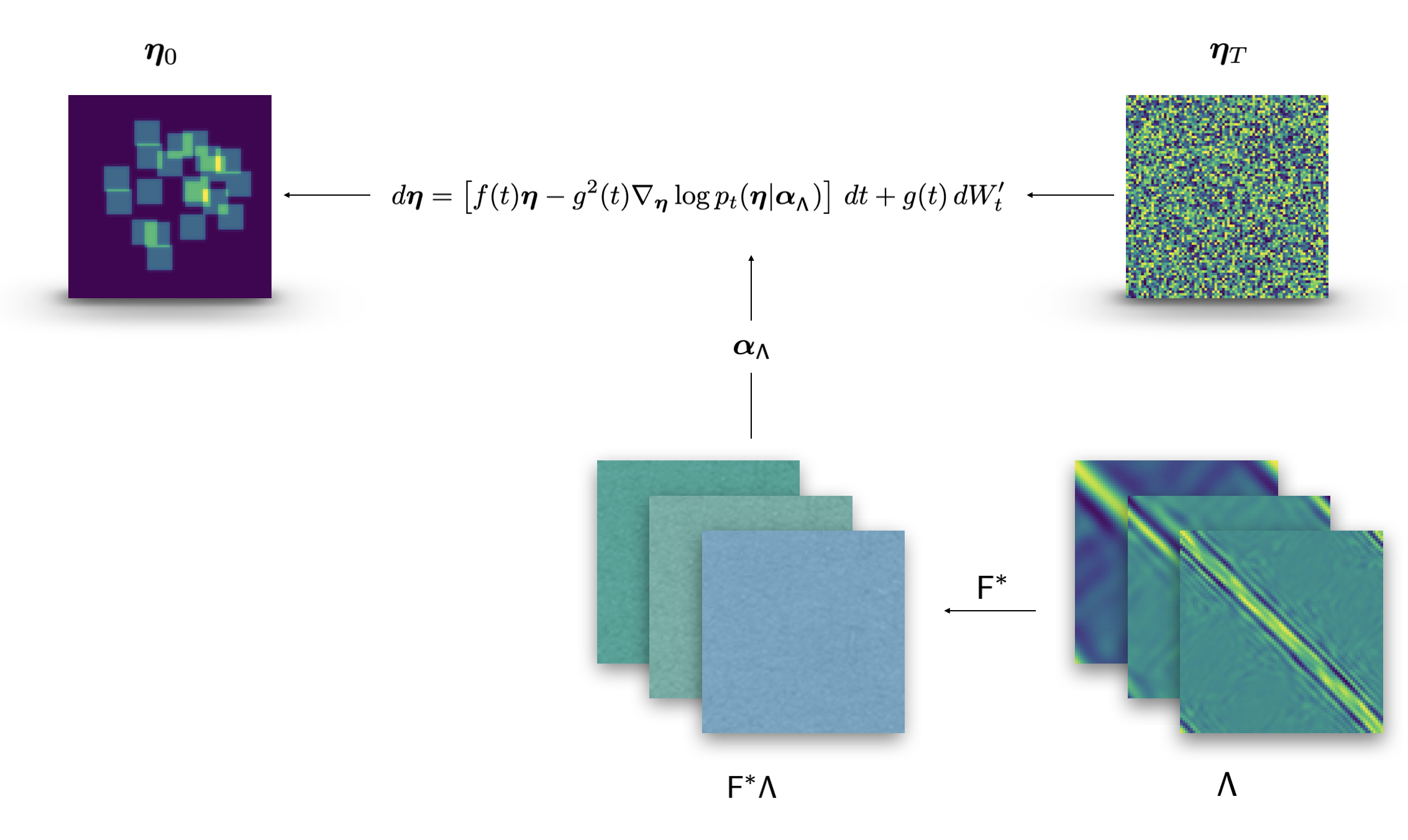
Figure 1: Sketch of the approach. The input data denoted by $\sf{\Lambda}$, a collection of scattered data at different frequency, is mapped to the reconstruction $\bm{\eta}_{0}$. The network $\sf{F}^{*}$ is used to map the input data to a latent representation, $\bm{\alpha}_{\sf{\Lambda}}=\sf{F}^{\star}\sf{\Lambda}$, which is then fed into the conditional score function, $\nabla_{\bm{\eta}}\log p_{t}(\bm{\eta}|\bm{\alpha}_{\sf{\Lambda}})$ of a diffusion model. To reconstruct the medium, we solve the Langevin equation backwards, using Gaussian noise as terminal condition.

In summary, our framework has the following highly desirable properties:

Highly Accurate Reconstruction: We show that our framework, is able to reconstruct the underlying medium accurately producing very sharp images even of objects with features below the diffraction limit, with around 1-2% of relative error, which is virtually indistinguishable to the naked eye. It outperforms other state-of-the-art models in the challenging cases involving multiple overlapping scatterers with strong multiple-scattering, and when the scatterers have features below the diffraction limit, such as diffraction corners.

Training Efficiency: We show that such high-accuracy reconstruction can be accomplished with a relatively low-sample complexity, while requiring only a modest amount of learnable parameters. This is achieved by relying on the rotational equivariance of the latent representation and the translation equivariance of the generative step. In addition, leveraging rank-structured neural networks, such as Butterfly Networks [25], to process the wideband data efficiently, allows us to further reduce the scaling of the number of parameters with respect to the target resolution of the reconstruction.

Low Computational Cost: We show that our framework has a relatively small computational complexity. This is achieved by relying on the symmetries of the problem, including respecting the information flow inherited from the filtered back-projection formula, and the the equivariance of the operators. In addition, we show that it is possible to further reduce the complexity by leveraging butterfly compression, albeit, with a small trade-off in accuracy.

Training Stability: The training stage is remarkably robust, particularly when compared to other inverse problem algorithm, which we inherit from the generative AI training pipelines.

Resilience to Noise: We show that our methodology is resilient to moderate measurement noise, is able to learn different distributions of datasets, and is able to handle scattered data from different discretization, with only a minor reduction on the accuracy.

1.2 Related Works

1.2.1 Classical Approaches

Many non-ML approaches for image reconstruction have been developed over the years. Due to the extensive literature we focus in problems that rely on optimization, and we refer the reader to [16, 50, 51] for reviews of analysis-based methods.

Among the earliest methods one we can find travel-time tomography [52, 53, 54]. Travel-time tomography reduces the inverse problem to a geometrical one of finding a metric [55]. In a nutshell, one assumes that rays propagate inside the unknown domain satisfying the minimum action principle following the unknown metric. By using the time that each ray takes to travel between points one can write a non-linear least-square problem [56], whose solution is used to estimate the wavespeed inside the medium. This technique can be cheaply implemented, however, it assumes that the wavespeed is smooth and the frequency of the propagating waves is high-enough to accept a ray approximation. Therefore, the reconstructions quickly deteriorate when highly heterogeneous media or multiple scatterers present.

Following the advent of modern computers, and their increasing capability of numerically solving the underlying PDEs, full-waveform inversion (FWI) was introduced [2] in the late 80’s. FWI recast the inverse problem as a PDE-constrained optimization problem, where the goal is to minimize the misfit between the real data and synthetic data that comes from the numerical solution of the governing PDE [46]. The main advantage with respect to other methods, is its capability of handling multiple scattering with ease.

Despite being considered the go-to classical technique for image reconstruction, particularly in geophysical exploration [18], it has some important drawbacks. First, the amount of computational power needed to compute the gradient inside the optimization loop is prohibitive. Even with state-of-the-art solvers [14, 57], the complexity of each iteration is superlinear [58] with respect to the number of unknowns to recover. Another drawback is the cycle-skipping phenomenon, which refers to the convergence to spurious local minima. This is a byproduct of the lack of convexity of the problem, and the lack of low-frequency data, which is usually daunting (and expensive) to acquire. Efforts to tackle this issue include adding regularization [59, 12], extrapolating the data to lower frequency [60], or modifying the problem to encourage robustness [61]. The last issue is the limitation in the resolution [62, 63] to recover fine-grained details, due to the diffraction limit.

1.2.2 Machine Learning Approaches

Most results produced by the classical approaches mentioned above are not yet desirable, thus, fueled by the development of modern ML tools, many ML approaches have been developed in recent years to bypass or attenuate the drawbacks of classical approaches. We divide them into two groups: deterministic and probabilistic approaches.

Deterministic

Generally speaking, most of ML-based methods used for inverse scattering employ a supervised trained neural network to regress the scatterer that uses scattered fields as the input data [27, 64, 65]. In order to be successful, ML approaches in inverse problems tend to integrate physical and/or mathematical properties of the problem at hand in the architecture of the neural network. These approaches have been proven more successful than their classical counterparts but they still have some limitations that prevent them to be fully applicable.

Some approaches, developed specifically for the inverse scattering problem, improve the performance of a classical approach by leveraging the available training data. In [66] the authors train a neural network to give a better initial guess to a Gauss-Newton iteration algorithm and have faster and more accurate convergence. On the other hand, in [13], wideband scattering data is deployed to approximate the inverse map. Very recently authors in [24], also seek to approximate the inverse map by leveraging wideband scattering data with an iterative refinement approach akin to a Neumann series developed in [67, 68]. Approaches that involve exploiting the physical structure of the problem, such as embedding rotational equivariant in the neural network construction for a homogeneous background, have also been examined [27, 29].

Although these methods sometimes produce satisfactory reconstructions, they also have significant drawbacks. Most important drawback is that deterministic ML models typically fail to provide any quantitative measurement of uncertainties, a task that has paramount of importance in reality. Additionally, these deterministic machine learning methods are highly sensitive to experimental configuration. Variations in frequency, and the number of transmitters and receivers, can all significantly impact the quality of the reconstruction.

Probabilistic

Probabilistic ML models automatically account for uncertainties, making them preferred for certain practical problems. Among probabilistic ML models, generative models are the most popular, offering multiple options to choose from: generative adversarial networks (GANs) [69, 70], variational autoencoders (VAE) [71], normalizing flows [72] and diffusion models [32]. Many of them have already been applied to solve inverse problems [35, 36].

Different generative models offer varying performance, each with its own strengths and weaknesses. For instance, GANs have been deployed to learn the prior, and GAN priors have been shown to outperform sparsity priors in some compressive sensing tasks with reduced sample complexity [73, 74, 75]. However, they face challenges in generalization, particularly when the online data is out-of-distribution. Moreover, GANs are prone to catastrophic forgetting, i.e., forgetting previously learned tasks while learning new ones [76]. Normalizing flow, another generative model, is also employed to solve inverse problems, either by training the prior or the posterior distribution in Bayes formula [37, 77]. The injectivity property of normalizing flows ensures zero representation error, enabling the recovery of any image, including those significantly out-of-distribution relative to the training set [78, 79, 80]. Numerical strategies are also integrated to progressively increase dimension from a low-dimensional latent space [77] for an enhanced computational efficiency. In addition to direct sampling, the variational inference framework, serving as an alternative to Bayesian posterior formulation, has been explored in the context of inverse scattering [81, 82, 83] using normalizing flows. This approach has shown promising experimental results, although it lacks extensive analytical support.

Score-based sampling is another generative modeling approach for solving inverse problems. Usually a score function is learned to denoise a Gaussian random variable to produce a sample from a desired probability measure. In the context of inverse problem, this probability measure takes the form of a conditional distribution, directing the training to focus on the conditional score function [43, 84]. Numerical strategies to improve computational efficiency have also been investigated. Notably, the work by [85] introduces an elegant tilted transport technique that exploits the quadratic structure of the log-likelihood function to enhance the convexity of the target distribution. When combined with a learned denoiser for the prior, this method is shown to reach the computational threshold in certain cases. None of the aforementioned work address equivariance structure inherent to the physical problem or examines its interaction with the training of the conditioning score function.

1.3 Outline

In Section 2, we present preliminary results. This includes the formulation of the inverse scattering problem and the associated filtered back-projection formula, and the Bayesian interpretation of PDE-constrained optimization. Section 3 briefly reviews some basics of score-based diffusion models, and the extension to sampling from conditional distributions. Section 4 is dedicated to the presentation of our proposed method that we term ‘wideband back-projection diffusion model’. This includes a specific factorization inspired by the filtered back-projection formula, with an examination of the mathematical properties of each component and their integration into the neural network design. This section also presents the major theoretical results of our work, demonstrating the required properties of the score function to ensure a certain equivariance structure. Finally, in Section 5, we provide ample numerical evidence showcasing the properties of the methodology.

2 Preliminaries

In this section, we provide a brief overview of the problem setup, and discuss some classical methods for addressing it. We present the filtered back-projection formula and highlight its properties that we will leverage in later sections. Finally, we introduce a Bayesian approach to solve this problem through posterior sampling, the numerical framework to be deployed in this work.

2.1 Physics Problem Setup

We focus on time-harmonic constant-density acoustic scattering in two dimensions, whose underlying physical model is given by the Helmholtz equation. Despite its simplicity, this model encapsulates the core challenges found in more complex models. In this case, the Helmholtz equation, the Fourier transform in time of the constant-density acoustic wave equation, is written as

$$\Delta u(\bm{x})+\omega^{2}n(\bm{x})u(\bm{x})=0\,,\quad\bm{x}\in\Omega\subset\mathbb{R}^{2}\,,$$ (1)

where $u$ is the total wave field, $\omega$ is the frequency, and $n$ is the refractive index. The domain of interest is $\Omega\subset\mathbb{R}^{2}$, and homogeneous background is set to be $n(\bm{x})=1$ for $\bm{x}\notin\Omega$. Define the perturbation $\eta(\bm{x})=n(\bm{x})-1$, we have $\text{supp}(\eta(\bm{x}))\subset\Omega$.

Forward Problem

For a given $n$ (or $\eta$), the forward problem involves solving for the scattered wave field resulting from the impulse response of the medium as it is impinged by a monochromatic plane wave,

$$u^{\text{in}}=e^{i\omega\bm{s}\cdot\bm{x}}\,,$$ (2)

where $\bm{s}\in\mathbb{S}^{1}$ is the direction of the incoming wave, and the scattered wave field $u^{\mathrm{sc}}$ is defined as

$$u^{\mathrm{sc}}=u-u^{\text{in}}\,.$$ (3)

Given that $u^{\text{in}}$ solves the Helmholtz equation in the background medium ($n(\bm{x})=1$), $u^{\mathrm{sc}}(\bm{x};\bm{s})$ satisfies

$$\begin{cases}\Delta u^{\mathrm{sc}}(\bm{x})+\omega^{2}(1+\eta(\bm{x}))u^{\mathrm{sc}}(\bm{x})=-\omega^{2}\eta(\bm{x})u^{\text{in}}\,,\\ \frac{\partial u^{\mathrm{sc}}}{\partial|\bm{x}|}-i\omega u^{\mathrm{sc}}=\mathcal{O}(|\bm{x}|^{-3/2})\text{ uniformly as }|\bm{x}|\to\infty\,.\end{cases}$$ (4)

The second equation is the Sommerfeld radiation condition, ensuring the uniqueness of the solution.

We select the detector manifold $D$ to be a circle of radius $R$ that encloses the domain of interest $\Omega$, i.e., $R>\text{radius}(\Omega)$. For each incoming direction $\bm{s}\in\mathbb{S}^{1}$ the data is given by sampling the scattered field with receivers located on $D$ and indexed by $\bm{r}\in\mathbb{S}^{1}$. This process yields the scattering data for each frequency $\omega$ as a function $\Lambda^{\omega}:[0,2\pi]^{2}\to\mathbb{C}$ such that

$$\Lambda^{\omega}(r,s)=u^{\mathrm{sc}}(R\bm{r};\bm{s})\,,$$ (5)

where $\bm{s}=(\cos(s),\sin(s))$, $\bm{r}=(\cos(r),\sin(r))$. We omit the dependence on $\omega$ on the right hand side when the context is clear.

Each refractive index field $\eta$ can be mapped to a set of scattering data $\Lambda^{\omega}$. This map is denoted the forward map: $\Lambda^{\omega}=\mathcal{F}^{\omega}[\eta]$. Figure 2 illustrates the setup of the forward problem and the data acquisition. In practice, one can obtain the scattering data produced by multiple impinging wave frequencies, and we denote $\bar{\Omega}$ the discrete set of chosen frequencies.

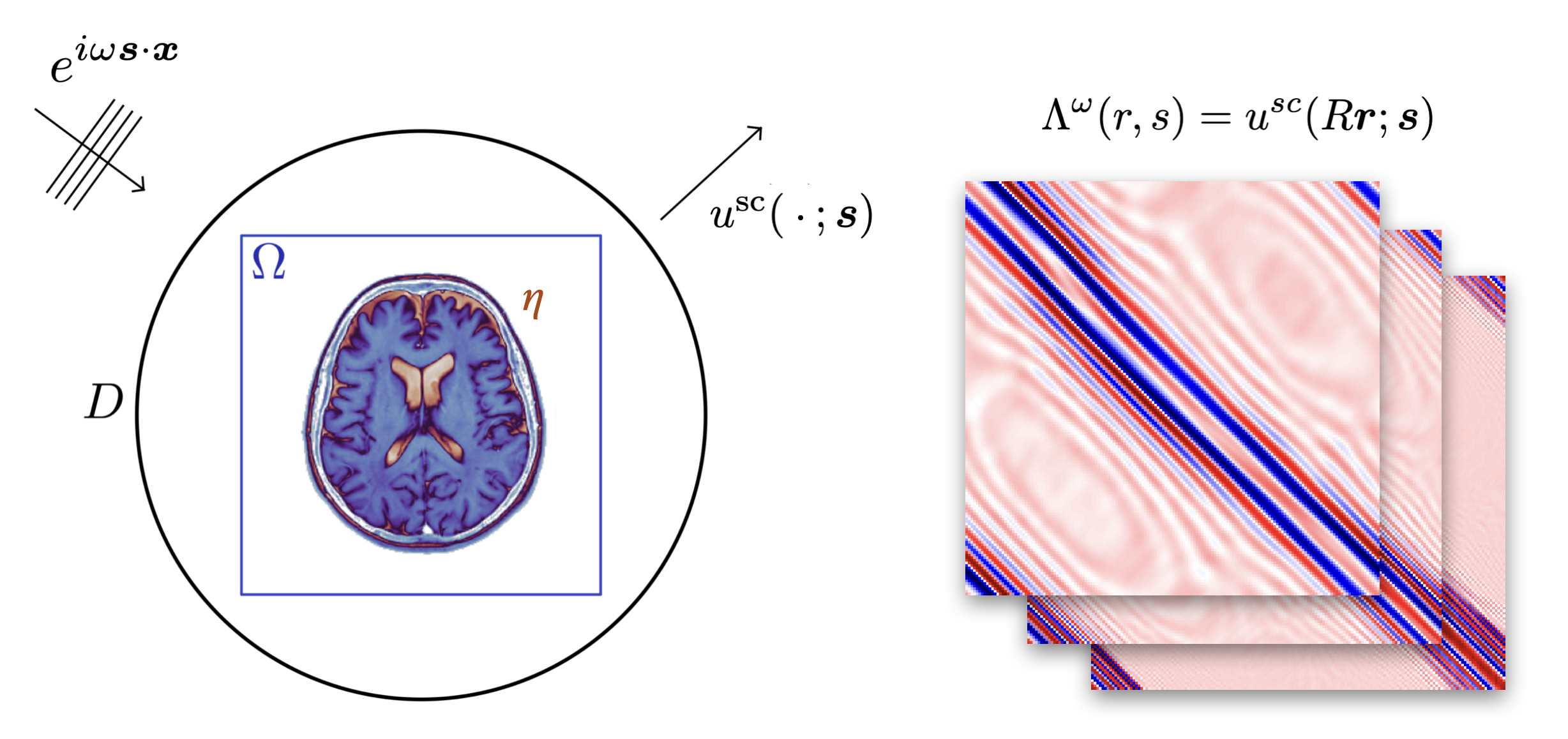
Figure 2: The plot on the left shows the setup for the inverse scattering problem: The perturbation $\eta$ is supported on the domain of interest $\Omega$. The media is impinged by a probing plane wave of frequency $\omega$ in the direction $\bm{s}$ and the scattered wave $u^{\mathrm{sc}}$ is collected. On the right, we show a typical scattering data $\Lambda^{\omega}(r,s)=u^{\mathrm{sc}}(R\bm{r};\bm{s})$.

Inverse Problem

The inverse problem is to revert the process and to reconstruct $\eta$ from $\Lambda^{\omega}$. This amounts to find:

$$\eta^{\ast}=\mathcal{F}^{-1}(\{\Lambda^{\omega}\}_{\omega\in\bar{\Omega}})\,.$$ (6)

We can recast the inverse problem as a PDE-constrained optimization problem that seeks to minimize the data misfit, i.e.,

$$\eta^{\ast}=\operatorname*{arg\,min}_{\eta}\sum_{\omega\in\bar{\Omega}}\|\Lambda^{\omega}-\mathcal{F}^{\omega}[\eta]\|^{2}\,,$$ (7)

where we consider the $L^{2}([0,2\pi]^{2})$ norm for the data misfit, namely:

$$\|\Lambda^{\omega}-\mathcal{F}^{\omega}\eta\|^{2}=\int_{[0,2\pi]^{2}}|\Lambda^{\omega}(r,s)-\left(\mathcal{F}^{\omega}\eta\right)(r,s)|^{2}\,dr\,ds\,.$$ (8)

This formulation seeks the configuration of $\eta$ that minimizes the misfit between the synthetic data generated by $\eta$ (solving PDE in (4)) and the observed scattering data $\Lambda^{\omega}$. When a single frequency is used, the objective function is highly non-convex, with a standard gradient-based optimization approach converging to spurious local minima, a phenomenon termed cycle-skipping. Setting $|\Omega|\neq 1$ to utilize wideband data is a strategy to stabilize optimization [18, 19]. The optimization problem (7) is typically solved using tailored gradient-based optimization techniques whose gradients are computed via adjoint-state methods [86]. Such optimization techniques either incorporate an explicit regularization term [87], or leverage sensitivity of (8) at different frequencies to solve (7) in a hierarchical fashion [18, 58].

2.2 Filtered Back-Projection

Linearizing the forward operator, $\mathcal{F}^{\omega},$ is instructive as it sheds light on the essential difficulties of this problem and naturally leads to the filtered back-projection formula. This formula has inspired many of the recent machine learning-based algorithms [29, 13, 26]. This formula also serves as an inspiration for our factorization to be presented in Section 4.

Using the classical Born approximation [88], in (4), we obtain that

$$u^{\mathrm{sc}}(\bm{x})=\omega^{2}\int_{\mathbb{R}^{2}}\Phi^{\omega}(\bm{x},\bm{y})\eta(\bm{y})e^{i\omega(\bm{s}\cdot\bm{y})}d\bm{y}\,,$$ (9)

where $\Phi^{\omega}$ is the Green’s function of the two-dimensional Helmholtz equation in a homogeneous medium, i.e., $\Phi^{\omega}$ solves

$$\left\{\begin{array}[]{ll}\displaystyle\left(\Delta+\omega^{2}\right)\Phi^{\omega}(\bm{x},\bm{y})=-\delta(\bm{x},\bm{y})&\text{ for }\bm{x}\in\mathbb{R}^{2}\,,\\ \displaystyle\lim_{|\bm{x}|\rightarrow\infty}|\bm{x}|^{1/2}\left(\frac{\partial}{\partial|\bm{x}|}-\mathrm{i}\omega\right)\Phi^{\omega}(\bm{x},\bm{y})=0\,.\end{array}\right.$$ (10)

Furthermore, we can use the classical far-field asymptotics of the Green’s function to express

$$u^{\mathrm{sc}}(R\bm{r})=-\omega^{2}\frac{e^{i\omega R}}{\sqrt{R}}\int_{\mathbb{R}^{2}}\eta(\bm{y})e^{i\omega(\bm{s}-\bm{r})\cdot\bm{y}}d\bm{y}+\mathcal{O}(R^{-3/2})\,.$$ (11)

Thus, up to a re-scaling factor and a phase change, the far-field pattern defined in (5) can be approximately written as a Fourier transform of the perturbation, viz.:

$$\Lambda^{\omega}(r,s)\approx F^{\omega}\eta=\int_{\mathbb{R}^{2}}e^{i\omega(\bm{s}-\bm{r})\cdot\bm{y}}\eta(\bm{y})d\bm{y}\,.$$ (12)

In this notation, $F^{\omega}$ is the linearized forward operator acting on the perturbation. In this linearized setting, solving the inverse problem in (8) using a single frequency $\omega$ with the linearized operator $F^{\omega}$ leads to the explicit solution

$$\eta^{*}=\left(F^{\omega}\right)^{\dagger}\Lambda^{\omega}\qquad\text{where}\quad\left(F^{\omega}\right)^{\dagger}=\left((F^{\omega})^{\ast}F^{\omega}\right)^{-1}(F^{\omega})^{\ast}\,.$$ (13)

However, $F^{\omega}$ is usually ill-conditioned, one routinely leverages Tikhonov-regularization with regularization parameter $\epsilon$, which results in the formula

$$\eta^{*}=\left(\left(F^{\omega}\right)^{*}F^{\omega}+\epsilon I\right)^{-1}\left(F^{\omega}\right)^{*}\Lambda^{\omega}.$$ (14)

This formula is referred to as filtered back-projection [89], and is optimal with respect to the $L^{2}$-objective. Concomitantly, as many other Tikhonov regularization, yield low-pass filtered estimates, particularly with large $\epsilon$. In practice, $\epsilon$ is chosen to be sufficiently large so as to remedy the ill-conditioning of the normal operator $\left(F^{\omega}\right)^{*}F^{\omega}$, but small enough not to damp the high-frequency content of the reconstruction.

This formula clearly states that there are two stages in the reconstruction. The first stage applies the back-scattering operator $(F^{\omega})^{\ast}$ to produce $\alpha^{\omega}$, the intermediate field:

$$\alpha^{\omega}\mathrel{\mathop{:}}=(F^{\omega})^{\ast}\Lambda^{\omega}\,.$$ (15)

This intermediate field can be computed explicitly following (12), up to a re-scaling factor, as:

$$\alpha^{\omega}(\bm{y})=(F^{\omega})^{*}\Lambda^{\omega}(\bm{y})=\int_{[0,2\pi]^{2}}e^{i\omega(\bm{r}-\bm{s})\cdot\bm{y}}\Lambda^{\omega}(r,s)\,dr\,ds\,.$$ (16)

Then the second stage maps $\alpha^{\omega}$ through the filtering operator to the final reconstruction of $\eta^{*}$.

The back-scattering operator and the filtering operator enjoy some mathematical symmetry, as outlined in the following propositions.

Proposition 2.1.

The back-scattering operator $(F^{\omega})^{\ast}:L^{2}([0,2\pi]^{2})\rightarrow L^{2}(\mathbb{R}^{2})$ is injective.

Proposition 2.2.

The back-scattering operator $(F^{\omega})^{\ast}:L^{2}([0,2\pi]^{2})\rightarrow L^{2}(\mathbb{R}^{2})$ satisfies rotational equivariance.

Proposition 2.3.

The filtering operator $\left((F^{\omega})^{\ast}F^{\omega}+\epsilon I\right)^{-1}$ that maps $\alpha^{\omega}$ to $\eta^{\ast}$ satisfies translational equivariance.

The proof for Proposition 2.1 is included in Appendix A.3. The precise definitions of rotational and translational equivariance are provided in [29], where the justifications for Propositions 2.2 and 2.3 are also detailed.

Remark: So far the method has been presented using single-frequency data and the reconstruction is usually ill-posed in this regime. In computation, data at additional frequencies are collectively used to stabilize the reconstruction [11]. In particular, a time-domain formulation known as the imaging condition yields a more stable reconstruction using the full frequency bandwidth formally resulting in

$$\eta^{*}=\int_{\mathbb{R}}\left(\left(F^{\omega}\right)^{*}F^{\omega}+\epsilon I\right)^{-1}\left(F^{\omega}\right)^{*}\Lambda^{\omega}d\rho(\omega)\,,$$ (17)

where $d\rho(\omega)$ is a density related to the frequency content of the probing wavelet. When the density is closely approximated by a discrete measure then

$$\eta^{*}\approx\sum_{\omega\in\bar{\Omega}}\left(\left(F^{\omega}\right)^{*}F^{\omega}+\epsilon I\right)^{-1}\left(F^{\omega}\right)^{*}\Lambda^{\omega}\rho(\omega)\,,$$ (18)

over a discrete set of frequencies $\bar{\Omega}$ and weights $\rho(\omega)$. We note that the selection of these frequencies, in addition to the optimal ordering in which the summation is computed under an iterative regime, remains an open question and an area of active research [58].

2.3 Discretization

We translate the discussion from the previous sections to the discrete setting. To streamline the notation, quantities in calligraphic fonts, such as $\mathcal{F}^{\omega}$, are used to denote nonlinear maps, while those in regular fonts, such as $F^{\omega}$ and $\Lambda^{\omega}$, are used to denote the linearized version. The quantities written in serif font, such as $\mathsf{F}^{\omega}$ and ${\sf\Lambda}^{\omega}$, are used to present the discretized version of the associated linear operators.

Since $\bm{s},\bm{r}\in\mathbb{S}^{1}$, we associate them with angles

$$\bm{s}=(\cos(s),\sin(s))\text{\quad and\quad}\bm{r}=(\cos(r),\sin(r))\,.$$ (19)

Numerically, the directions of sources and detectors are represented by the same uniform grid in $\mathbb{S}^{1}$ with $n_{\mathrm{sc}}$ grid points given by

$$s_{j},r_{j}=\frac{2\pi j}{n_{\mathrm{sc}}},\ j=0,\dots,n_{\mathrm{sc}}-1\,.$$ (20)

Using this setting, the discrete scattering data ${\sf\Lambda}^{\omega}$ takes its values on the tensor of both grids with complex values, which are decomposed in their real and imaginary parts

$${\sf\Lambda}^{\omega}={\sf\Lambda}^{\omega}_{R}+i{\sf\Lambda}^{\omega}_{I}\in\mathbb{C}^{n_{\mathrm{sc}}\times n_{\mathrm{sc}}}\,.$$ (21)

We set the physical domain to be $\Omega=[-0.5,0.5]^{2}$ and use a Cartesian mesh of $n_{\eta}\times n_{\eta}$ grids. As a consequence, $\eta(\bm{x})$ is represented as a matrix: $\bm{\eta}\in\mathbb{R}^{n_{\eta}\times n_{\eta}}$ indexed by $i,j\in\mathbb{N}_{\eta}$ where $\mathbb{N}_{\eta}=\{0,1,\dots,n_{\eta}-1\}$ is the collection of grid points. In this form, $\bm{\eta}_{(i,j)}$ represents $\eta(\bm{x})$ evaluated on the Cartesian mesh. The intermediate field $\alpha^{\omega}(\bm{x})$ also lies in the physical domain, so it is discretized as a matrix: ${\bm{\alpha}^{\omega}\in\mathbb{R}^{n_{\eta}\times n_{\eta}}}$ the same way as $\bm{\eta}$.

Upon this discretization, all operators, $\mathcal{F}^{\omega}$, $F^{\omega}$ and $(F^{\omega})^{\ast}$ have their discrete counterparts. More specifically, we denote $\mathcal{F}_{d}^{\omega}:\mathbb{R}^{n_{\eta}\times n_{\eta}}\rightarrow\mathbb{C}^{n_{\mathrm{sc}}\times n_{\mathrm{sc}}}$, $\mathsf{F}^{\omega}:\mathbb{R}^{n_{\eta}\times n_{\eta}}\rightarrow\mathbb{C}^{n_{\mathrm{sc}}\times n_{\mathrm{sc}}}$ and $(\mathsf{F}^{\omega})^{\ast}:\mathbb{C}^{n_{\mathrm{sc}}\times n_{\mathrm{sc}}}\rightarrow\mathbb{R}^{n_{\eta}\times n_{\eta}}$ the discretized forward map, linearized forward map, and back-scattering operator, respectively.

2.4 Bayesian Sampling

Even though the reconstruction is unique, it has been shown to be unstable, particularly as the frequency increases [11]. This poses a conundrum: reconstructions usually require higher frequency data to capture small-grained features, which are of great interest for downstream applications, but the reconstruction itself becomes increasingly unstable. This issue is further compounded in realistic scenarios where data always contains measurement errors and models present epistemic uncertainties. Thus, one alternative is to treat this problem under the Bayesian umbrella. Namely, one wants to compute, or have access to, the posterior distribution drawn from the Bayes’ rule [90], i.e.,

$$p(\bm{\eta}|{\sf\Lambda}^{\omega})\propto p(\bm{\eta})p({\sf\Lambda}^{\omega}|\bm{\eta})\,.$$ (22)

with $p(\bm{\eta})$ being the prior distribution, serving as a regularization term, and $p({\sf\Lambda}^{\omega}|\bm{\eta})$ serving as the likelihood function. The reconstruction can be carried out by finding the maximum a posteriori (MAP) estimation:

$$\bm{\eta}^{*}=\operatorname*{arg\,max}_{\bm{\eta}}p(\bm{\eta}|{\sf\Lambda}^{\omega})\,.$$ (23)

The prior distribution is usually computed based on expected properties, such as sparse representation in Fourier space, of piece-wise constant scatterers.

Computing this probability is intractable, but one can nevertheless sample from it. A standard strategy is to design a Markov chain whose invariant measure recovers the target distribution. In this context, the target distribution is the posterior distribution (22). If the Markov chain has this property, any random initialization for $\bm{\eta}$, after going through the chain along long enough pseudo-time, can potentially be viewed as a sample from the target distribution. There are many choices for designing this Markov chain, and one of the most popular is the Langevin-type:

$$d\bm{\eta}=-\nabla_{\bm{\eta}}\log p(\bm{\eta}|{\sf\Lambda}^{\omega})dt+\sqrt{2}dW_{t}\,,$$ (24)

where $dW_{t}$ is a Wiener process.

As made evident in (24), knowing the score function $\nabla_{\bm{\eta}}\log p(\bm{\eta}|{\sf\Lambda}^{\omega})$ is crucial for sampling from the posterior distribution. It is often rare to find examples where the score function can be computed explicitly. Numerically, one seeks to find its numerical approximation. A typical assumption involves considering a Gaussian approximation to the misfit; specifically, assuming $\Sigma$, a positive definite matrix, is the covariance matrix of the measurement error, we derive:

$$p({\sf\Lambda}^{\omega}|\bm{\eta})\propto\exp{\left(\frac{1}{2}(\mathcal{F}^{\omega}_{d}[\bm{\eta}]-{\sf\Lambda}^{\omega})^{\intercal}\Sigma^{-1}(\mathcal{F}^{\omega}_{d}[\bm{\eta}]-{\sf\Lambda}^{\omega})\right)}\,.$$ (25)

Throughout the paper, without loss of generality, we simplify the formulation by assuming $\Sigma=\sigma^{2}\bm{I}$. In this case we can integrate (22) with (25) to have

$$d\bm{\eta} =-\nabla_{\bm{\eta}}\log p({\sf\Lambda}^{\omega}|\bm{\eta})\,dt+\nabla_{\bm{\eta}}\log p(\bm{\eta})\,dt+\sqrt{2}dW_{t}\,,$$ (26)

$$=-\frac{1}{2\sigma^{2}}\nabla_{\bm{\eta}}\|\mathcal{F}_{d}^{\omega}[\bm{\eta}]-{\sf\Lambda}^{\omega}\|^{2}\,dt+\nabla_{\bm{\eta}}\log p(\bm{\eta})\,dt+\sqrt{2}dW_{t}\,,$$

where the two terms in the velocity field respectively represent the gradient flow induced by the misfit function in (8), and a regularization term.

However, in what follows, we argue that we can learn this conditional score function directly leveraging state-of-the-art generative AI tools.

3 Denoising Diffusion Probabilistic Modeling (DDPM)

The goal of score-based generative models is to be able to sample from a target data distribution using a sample from an easy-to-sample distribution, such as high-dimensional Gaussian, with a progressive transformation of the sample. Theoretically this procedure is backed by a simple observation that sequentially corrupting a sample of any distribution with increasing noise produces a sample drawn from a Gaussian distribution. Score-based generative model is to revert this process, and produce a sample from the target distribution by “denoise" a Gaussian sample. Two mathematically equivalent computational frameworks are: score matching with Langevin dynamics (SMLD) [91], which estimates the score (i.e., the gradient of the log probability density with respect to data), or DDPM [32], which trains a sequence of probabilistic models to reverse the noise corruption of our data.

In this section we introduce the main ideas behind DDPM; from its mathematical foundation, to how we can extend it for a target conditional distribution, including some practical considerations [92, 93, 94] that render the algorithm more efficient.

3.1 Mathematical Foundation

The mathematical foundation of DDPM lies on the well known fact that a simple stochastic process can map an arbitrarily complicated distribution ($p_{\text{data}}$) to a simple Gaussian Normal. To see this, we start off with the classical Ornstein–Uhlenbeck (OU) process [95],

$$\,d\bm{\eta}_{t}=-\bm{\eta}_{t}\,dt+\sqrt{2}\,dW_{t}\,,\quad\bm{\eta}_{0}\sim p_{\text{data}}\,,$$ (27)

where $W_{t}$ is a Brownian motion. The Feynman-Kac formula [96] suggests that the law of $\bm{\eta}$ solves the following Fokker-Planck equation:

$$\partial_{t}p_{t}(\bm{\eta})=\nabla_{\bm{\eta}}\cdot(\bm{\eta}p_{t}(\bm{\eta}))+\Delta_{\bm{\eta}}p_{t}(\bm{\eta})\,,\quad\text{with}\quad p_{0}=p_{\text{data}}\,.$$ (28)

It is a classical result that in the long time limit as $t\to\infty$,

$$p_{\infty}\propto e^{-\frac{\|\bm{\eta}\|^{2}}{2}}\propto\mathcal{N}(\bm{\eta};\bm{0},\bm{I})\,,$$ (29)

where $\mathcal{N}$ stands for normal distribution with mean and variance presented as the last two parameters. This derivation means that (28) maps $p_{\text{data}}$ to a standard Gaussian. Equivalently, a sample $\bm{\eta}$ drawn from $p_{\text{data}}$, through the OU process, become a Gaussian sample.

DDPM seeks to revert this process. From (28), by letting $t=T-\tau$, a simple derivation gives:

$$\partial_{\tau}p_{T-\tau}(\bm{\eta}) =-\nabla_{\bm{\eta}}\cdot(\bm{\eta}p_{T-\tau}(\bm{\eta}))-\Delta_{\bm{\eta}}p_{T-\tau}(\bm{\eta})$$ (30)

$$=-\nabla_{\bm{\eta}}\cdot(p_{T-\tau}(\bm{\eta})(\bm{\eta}+2\nabla_{\bm{\eta}}\log{p_{T-\tau}}(\bm{\eta})))+\Delta_{\bm{\eta}}p_{T-\tau}(\bm{\eta})$$

$$=-\nabla_{\bm{\eta}}\cdot(p_{T-\tau}(\bm{\eta})(\bm{\eta}+2\nabla_{\bm{\eta}}\log{p_{t}}(\bm{\eta})))+\Delta_{\bm{\eta}}p_{T-\tau}(\bm{\eta})\,,$$

where we term $\nabla_{\bm{\eta}}\log{p_{t}}$ the score function of the process. These dynamics can be represented by the associated SDE as well:

$$d\tilde{\bm{\eta}}_{T-\tau}=(\tilde{\bm{\eta}}_{T-\tau}+2\nabla_{\bm{\eta}}\log{p_{t}}(\tilde{\bm{\eta}}_{T-\tau}))\,d\tau+\sqrt{2}\,dW_{T-\tau}^{\prime}\,,$$ (31)

Change the time variable $t=T-\tau$ back:

$$d\tilde{\bm{\eta}}_{t}=-(\tilde{\bm{\eta}}_{t}+2\nabla_{\bm{\eta}}\log{p_{t}}(\tilde{\bm{\eta}}_{t}))\,dt+\sqrt{2}\,dW_{t}^{\prime}\,,$$ (32)

where $W_{t}^{\prime}$ is a Brownian motion. Clearly, $p_{T-\tau}$ reverts the process of $p_{t}$ and thus maps a Gaussian normal distribution (in the $T\to\infty$ limit) to $p_{\text{data}}$. Therefore, a sample $\tilde{\bm{\eta}}_{T}\sim\mathcal{N}(\,\cdot\,;\bm{0},\bm{I})$ and runs through (32) approximately produces a sample from $p_{\text{data}}$ at $t=0$.

3.2 Practical Considerations

It is straightforward to see that the OU process studied in Section 3.1 is not the only dynamics that links the target distribution $p_{\text{data}}$ to $\mathcal{N}(\,\cdot\,;\bm{0},\bm{I})$. To speed up the dynamics, one has the freedom to adjust the velocity field and the strength of the Brownian motion. In particular, define $f$ as the drift coefficient, and $g$ the diffusion coefficient, we let $\bm{\eta}$ solve

$$d\bm{\eta}_{t}=f(t)\bm{\eta}_{t}\,dt+g(t)\,dW_{t}\,,\quad\bm{\eta}_{0}\sim p_{\text{data}}\,,$$ (33)

with $W_{t}$ being the standard Wiener process, then its law satisfies:

$$\partial_{t}p_{t}(\bm{\eta})=-\nabla_{\bm{\eta}}\cdot\left(\bm{\eta}f(t)p_{t}(\bm{\eta})\right)+\frac{1}{2}g^{2}(t)\Delta_{\bm{\eta}}p_{t}(\bm{\eta})\,,\quad\text{with}\quad p_{0}=p_{\text{data}}\,.$$ (34)

The solution to this PDE is:

$$p_{t}(\bm{\eta})=\int p_{\text{data}}(\bm{\eta}_{0})p_{0t}(\bm{\eta}|\bm{\eta}_{0})d\bm{\eta}_{0}\propto(p_{\text{data}}*\mathcal{N}(\,\cdot\,;\bm{0},\sigma^{2}(t)\bm{I}))\left(\frac{\bm{\eta}}{s(t)}\right)\,,$$ (35)

where the second equation comes from change of variables, and $p_{0t}$ is the Green’s function:

$$p_{0t}(\bm{\eta}|\bm{\eta}_{0})=\mathcal{N}(\bm{\eta};s(t)\bm{\eta}_{0},s^{2}(t)\sigma^{2}(t)\bm{I})\,.$$ (36)

The $(s,\sigma)$ pair is uniquely determined by the $(f,g)$ pair:

$$\begin{cases}s(t)=\exp\left(\int_{0}^{t}f(\xi)\,d\xi\right)\\ \sigma(t)=\sqrt{\int_{0}^{t}\frac{g(\xi)^{2}}{s(\xi)^{2}}\,d\xi}\end{cases}\,,\quad\text{and equivalently}\quad\begin{cases}f(t)=\frac{\dot{s}(t)}{s(t)}\\ g(t)=s(t)\sqrt{2\dot{\sigma}(t)\sigma(t)}\end{cases}\,.$$ (37)

The flexibility of adjusting $f$ and $g$ allows us to seek for dynamics that can drive $p_{\text{data}}$ to a Gaussian faster than the simple OU process. In particular, suppose we wish $p_{T}\approx\mathcal{N}(\,\cdot\,;\bm{0},C^{2}\bm{I})$ at a finite $T$ for a prefixed $C$, one only needs to set:

$$\lim_{t\to T}\sigma(t)=C\,,\quad\lim_{t\to T}s(t)=0\quad\text{so that}\quad\lim_{t\to T}p_{t}(\bm{\eta})=(\delta_{0}\ast\mathcal{N}(\,\cdot\,;\bm{0},C^{2}\bm{I}))(\bm{\eta})=\mathcal{N}(\bm{\eta};\bm{0},C^{2}\bm{I})\,.$$ (38)

Having $s(t=T)=0$ can introduce singularity in $p_{\text{data}}\left(\frac{\bm{\eta}}{s(t)}\right)$. To avoid numerical difficulties, we can relax it to be a very small number. One such example is to set

$$s(t)=\frac{1}{\sqrt{\sigma^{2}(t)+1}}\,,\quad\text{with}\quad\sigma(t)=\tan\left(t_{\text{max}}t/T\right)\,,\quad t_{\max}=\arctan(C)\,,$$ (39)

so that at $t=T$, $\sigma(T)=C$ and $s(T)=\frac{1}{\sqrt{C^{2}+1}}\ll 1$ for $C\gg 1$. This noise schedule $\sigma(t)$ was proposed in [97]. The scaling factor $s(t)$ follows from the variance-preserving formulation proposed in [92]. These are the strategies we follow in our simulations.

All these choices of drift and diffusion coefficients provide links between the target distribution $p_{\text{data}}$ with a Gaussian. So similar to (30) and (32), the reverse process that depends on the knowledge of the score function can be written as:

$$d\tilde{\bm{\eta}}_{t}=\left[f(t)\tilde{\bm{\eta}}_{t}-g^{2}(t)\nabla_{\bm{\eta}}\log p_{t}(\tilde{\bm{\eta}}_{t})\right]\,dt+g(t)\,dW_{t}^{\prime}\,,\quad\tilde{\bm{\eta}}_{T}\sim\mathcal{N}(\,\cdot\,;\bm{0},C^{2}\bm{I})\,.$$ (40)

It provides a sample at $t=0$: $\tilde{\bm{\eta}}_{0}\sim p_{\text{data}}$.

3.3 Score function learning

The success of running (40) to process a desired sample hinges on the availability of the score function. However, it is typically unknown and needs to be learned from data in the offline training stage. To do so, it is conventional to parameterize it using a neural network and learn the weights using samples of the target distribution.

To formulate the learning process through an objective function, we will recognize that the score function can be re-written by a conditional mean, and theoretically this conditional mean serves as a global optimizer of a specially designed loss function. To see so, we first rewrite (35). For any $\bm{\eta}_{0}\sim p_{\text{data}}$:

$$\bm{\eta}_{t}=s(t)\bm{\eta}_{0}+\bm{\varepsilon}_{t}\,,\quad\text{with}\quad\bm{\varepsilon}_{t}\sim\mathcal{N}(\,\cdot\,;\bm{0},s^{2}(t)\sigma^{2}(t)\bm{I})\,.$$ (41)

This presentation essentially writes $\bm{\eta}_{t}$ as a noised version of $\bm{\eta}_{0}$. To denoise $\bm{\eta}_{t}$ back to $\bm{\eta}_{0}$, we deploy the Tweedie’s formula [98, 99]:

$$\mathbb{E}[\bm{\eta}_{0}|\bm{\eta}_{t}]=\frac{\bm{\eta}_{t}}{s(t)}+s(t)\sigma^{2}(t)\nabla_{\bm{\eta}}\log{p_{t}(\bm{\eta}_{t})}\quad\Rightarrow\quad\nabla_{\bm{\eta}}\log{p_{t}}(\bm{\eta}_{t})=\frac{\mathbb{E}[\bm{\eta}_{0}|\bm{\eta}_{t}]-\bm{\eta}_{t}/s(t)}{s(t)\sigma^{2}(t)}\,.$$ (42)

Here the conditional mean is defined as:

$$\mathbb{E}[\bm{\eta}_{0}|\bm{\eta}_{t}]=\int\bm{\eta}_{0}p(\bm{\eta}_{0}|\bm{\eta}_{t})d\bm{\eta}_{0}=\frac{1}{p_{t}(\bm{\eta}_{t})}\int\bm{\eta}_{0}p_{0t}(\bm{\eta}_{t}|\bm{\eta}_{0})p_{\text{data}}(\bm{\eta}_{0})d\bm{\eta}_{0}\,,$$ (43)

where we have used the Bayes’ formula in the second equation. Noting this conditional mean is to recover the original signal $\bm{\eta}_{0}$ conditioned on a noisy version $\bm{\eta}_{t}$, and thus the term is interpreted as a denoiser. Equation (42) suggests that the computation of the score function can now be translated to the computation of $\mathbb{E}[\bm{\eta}_{0}|\bm{\eta}_{t}]$ in (43).

Remarkably, this conditional mean (43) is closely related to the optimizer of the following objective functional:

$$\mathcal{L}(D;\sigma)=\mathbb{E}_{\bm{\eta}\sim p_{\text{data}}}\mathbb{E}_{\bm{n}\sim\mathcal{N}(\,\cdot\,;\bm{0},\sigma^{2}\mathbf{I})}\left\|D(\bm{\eta}+\bm{n})-\bm{\eta}\right\|_{2}^{2}\,.$$ (44)

For a fixed $\sigma$, (44) maps a function of $\bm{\eta}$ to a non-negative number. Noting its quadratic and convex form, we derive its optimizer through the first critical condition. For every $t$, with $\sigma(t)$ fixed, setting:

$$\left.\frac{\delta\mathcal{L}}{\delta D}\right|_{\mathbb{E}[\bm{\eta}_{0}|s(t)\cdot]}=0\quad\Rightarrow\quad\mathbb{E}\left[\bm{\eta}_{0}|s(t)\cdot\right]=\operatorname*{arg\,min}\mathcal{L}(D;\sigma(t))\,.$$ (45)

Numerically, given samples of $p_{\text{data}}$ and $\bm{n}$ drawn from Gaussian distribution, the $\mathbb{E}$ in $\mathcal{L}$ is replaced by its empirical mean to define $\mathcal{L}_{e}$. Letting $D_{\bm{\Theta}}$, a neural network parameterized by $\bm{\Theta}$, be the minimizer of this empirical objective functional,

$$D_{\bm{\Theta}}(\,\cdot\,;\sigma)=\operatorname*{arg\,min}_{D_{\bm{\Theta}^{\prime}}}\mathcal{L}_{e}(D_{\bm{\Theta}^{\prime}};\sigma)\,,$$ (46)

then considering (45), $\forall t$, we have:

$$\mathbb{E}\left[\bm{\eta}_{0}|\bm{\eta}_{t}\right]\approx D_{\bm{\Theta}}\left(\frac{\bm{\eta}_{t}}{s(t)};\sigma(t)\right)\,.$$

The $\approx$ sign accounts for the failure of finding global optimum of (46), lack of approximation power of the neural network feasible set, and the empirical approximation of $\mathcal{L}$ by $\mathcal{L}_{e}$.

This numerical conditional mean $D_{\bm{\Theta}}\left(\frac{\bm{\eta}_{t}}{s(t)};\sigma(t)\right)$ then is integrated in the score-function formula (42) to enter the online stage for drawing a sample. We prepare $\bm{\eta}_{T}\sim\mathcal{N}(\,\cdot\,;\bm{0},C^{2}\bm{I})$ and run the following dynamics:

$$d\bm{\eta}_{t}=\left[\frac{\dot{s}(t)}{s(t)}\bm{\eta}_{t}-2s^{2}(t)\dot{\sigma}(t)\sigma(t)\frac{D_{\bm{\Theta}}(\bm{\eta}_{t}/s(t);\sigma(t))-\bm{\eta}_{t}/s(t)}{s(t)\sigma^{2}(t)}\right]\,dt+s(t)\sqrt{2\dot{\sigma}(t)\sigma(t)}\,dW_{t}^{\prime}\,,$$ (47)

from $t=T$ back to $t=0$. The output $\bm{\eta}_{0}$ provides an approximate sample from $p_{\text{data}}$.

3.4 Conditional Diffusion

In the context of the inverse scattering problem, as presented in Section 2.4, and (24), we are given the scattering data ${\sf\Lambda}^{\omega}$, and aim to draw a sample from the target distribution $p(\,\cdot\,|{\sf\Lambda}^{\omega})$. As a consequence, both the offline training and online drawing processes are conducted in this conditioned setting.

In the offline training stage, we run the optimization (46) with $p_{\text{data}}$ replaced by $p(\,\cdot\,|{\sf\Lambda}^{\omega})$. The output of the optimization formulation provides the approximation to the score function:

$$D_{\bm{\Theta}}\left(\frac{\bm{\eta}}{s(t)};{\sf\Lambda}^{\omega},\sigma(t)\right)\approx\frac{\bm{\eta}}{s(t)}+s(t)\sigma^{2}(t)\nabla_{\bm{\eta}}\log{p_{t}}(\bm{\eta}|{\sf\Lambda}^{\omega})\,.$$ (48)

With this knowledge in hand, in the online drawing, we prepare $\bm{\eta}_{T}\sim\mathcal{N}(\,\cdot\,;\bm{0},C^{2}\bm{I})$, and run reverse-time SDE [92] as

$$d\bm{\eta}_{t}=\left[\frac{\dot{s}(t)}{s(t)}\bm{\eta}_{t}-2s^{2}(t)\dot{\sigma}(t)\sigma(t)\frac{D_{\bm{\Theta}}(\bm{\eta}_{t}/s(t);{\sf\Lambda}^{\omega},\sigma(t))-\bm{\eta}_{t}/s(t)}{s(t)\sigma^{2}(t)}\right]\,dt+s(t)\sqrt{2\dot{\sigma}(t)\sigma(t)}\,dW_{t}^{\prime}\,,$$ (49)

from $t=T$ up to $t=0$. The output is a sample from the target $p(\,\cdot\,|{\sf\Lambda}^{\omega})$. The choices of $(s(t),\sigma(t))$ are consistent to previously defined in (39).

4 Wideband Back-Projection Diffusion Model

In this section, we integrate all the techniques presented above and we tailor them to solve the inverse scattering problem. More specifically, we aim to infer $\bm{\eta}$ from the knowledge of $\{{\sf\Lambda}^{\omega}\}_{\omega\in\bar{\Omega}}$ using the Bayesian framework introduced in Section 2.4. This involves drawing a sample from the posterior distribution using the DDPM framework:

$$\bm{\eta}^{\ast}\sim p(\bm{\eta}|\{{\sf\Lambda}^{\omega}\}_{\omega\in\bar{\Omega}})\,.$$ (50)

The dataset used to learn this posterior distribution is denoted

$$(\bm{\eta},\{{\sf\Lambda}^{\omega}\}_{\omega\in\bar{\Omega}})\sim p_{\text{data}}\,,$$ (51)

and, when context is clear, $p_{\text{data}}(\bm{\eta})$ denotes the marginal distribution. For the sake of brevity, we will omit the frequency $\omega$ from the discussion unless necessary. Particularly, in presence of the wideband data $\{{\sf\Lambda}^{\omega}\}_{\omega\in\bar{\Omega}}$, with an abuse of notation, we denote

$${\sf\Lambda}=\{{\sf\Lambda}^{\omega}\}_{\omega\in\bar{\Omega}}\quad\text{ and }\quad\bm{\alpha}_{\sf\Lambda}=\{\bm{\alpha}^{\omega}_{{\sf\Lambda}}\}_{\omega\in\bar{\Omega}}\,.$$ (52)

We recall that the inverse scattering problem, as presented in Section 2.2, is composed of two stages: the back-scattering and the filtering, see (14). These two stages exhibit very different structures, as discussed in Propositions 2.2 and 2.3. This structural difference suggests these two operations should be treated separately, thus inducing our factorization into a two-stage reconstruction:

• mimics the back-scattering operation and deterministically reconstructs the intermediate field $\bm{\alpha}_{\sf\Lambda}$, the discrete form of:

  $$\alpha_{\Lambda}(\bm{y})=F^{*}\Lambda(\bm{y})=\int_{[0,2\pi]^{2}}e^{i\omega(\bm{r}-\bm{s})\cdot\bm{y}}\Lambda(r,s)\,dr\,ds\,,$$ (53)

• mimics the filtering process and draws a sample $\bm{\eta}$ using DDPM, as defined by:

  $$d\bm{\eta}=\left[f(t)\bm{\eta}-g^{2}(t)\nabla_{\bm{\eta}}\log p_{t}(\bm{\eta}|\bm{\alpha}_{\sf\Lambda})\right]\,dt+g(t)\,dW_{t}^{\prime}\,$$ (54)

  where $\nabla_{\bm{\eta}}\log p_{t}(\bm{\eta}|\bm{\alpha}_{\sf\Lambda})$ will be termed the physics-aware score function.

Proposition 2.1 states that $F^{\ast}$ is injective, thus it is invertible within its range. Assuming its discrete version $\mathsf{F}^{\ast}$ enjoys the same property, then the conditional distribution satisfy $p(\bm{\eta}|{\sf\Lambda})=p(\bm{\eta}|(\mathsf{F}^{\ast})^{-1}\bm{\alpha}_{\sf\Lambda})$. Throughout the paper, we shorten the notation to be $p(\bm{\eta}|\bm{\alpha}_{\sf\Lambda})$.

This two-stage separation will be implemented in both the offline learning stage and the online sampling stage. In the offline learning stage, two neural networks will be independently developed to capture the back-scattering and filtering process respectively. The composite neural network maps the given data ${\sf\Lambda}$ to the physics-aware score function $\nabla_{\bm{\eta}}\log p_{t}(\bm{\eta}|\bm{\alpha}_{\sf\Lambda})$. The weights of the entire neural network are learned from $p_{\text{data}}$. Then, in the online stage, given any ${\sf\Lambda}$, we can produce a sample $\bm{\eta}$ by running (53)-(54) with the learned physics-aware score function $\nabla_{\bm{\eta}}\log p_{t}(\bm{\eta}|\bm{\alpha}_{\sf\Lambda})$.

To best follow the structure of the back-scattering and the filtering operators, we need to integrate the rotational equivariance and translational equivariance into the neural network architecture. To build in rotational equivariance to represent the back-scattering operator is straightforward, and we discuss it in Section 4.1. The translational equivariance of the filtering operator needs to be translated to the associated property for the score function, as seen in (54), is detailed in Section 4.2. Finally, to enhance training efficiency and quality, we employ an off-the-shelf preconditioned framework [93], which is elaborated upon in Section 4.3. The diagram of the approach is illustrated in Figure 1.

4.1 Representation of the Back-Scattering Operator

According to Proposition 2.2, the back-scattering operator is rotational equivariant. Therefore, we are to design a neural network, denoted as $F_{\bm{\Theta}_{1}}$, that preserves this rotational equivariance property to achieve:

$$\bm{\alpha}_{\sf\Lambda}\approx F_{\bm{\Theta}_{1}}(\sf\Lambda)\,.$$ (55)

Several choices are available:

Uncompressed Rotationally Equivariant Model (EquiNet)

The back-scattering operator, when expressed in polar coordinates $\bm{y}=(\rho\cos\theta,\rho\sin\theta)$, is formulated as:

$$[F^{*}\Lambda](\theta,\rho)=\int_{[0,2\pi]}\underbrace{e^{i\omega\rho\cos(r)}}_{\text{kernel }K^{\omega}}\bigg{(}\int_{[0,2\pi]}\underbrace{e^{-i\omega\rho\cos(s)}}_{\text{kernel }\overline{K^{\omega}}}\Lambda^{\omega}(r+\theta,s+\theta)\,ds\bigg{)}\,dr\,.$$ (56)

A notable observation detailed in [29] is that the rotational equivariance is preserved regardless of the form of $K^{\omega}$ and thus the integral kernel $K^{\omega}=e^{i\omega\rho\cos(t)}$ can be replaced by any other function. Numerically this integral kernel is modeled by a neural network that outputs a function of $(\rho,t)$. When this NN happens to output $K^{\omega}$, the analytical back-scattering operator is recovered. This whole approach of utilizing the formulation of (56) to preserve rotational equivariance is hence termed “EquiNet."

Compressed Rotationally Equivariant Model (B-EquiNet)

B-EquiNet is an extension of EquiNet and aims at reducing computational complexity, with the “B" standing for butterfly, drawing inspiration from the butterfly factorization [100]. This factorization is an economical presentation of a two-dimensional function and saves memory cost. The authors in [29] studied the butterfly structure of the integral kernel $K^{\omega}=e^{i\omega\rho\cos(t)}$ and integrated this structure in building the NN representation.

Remark 4.1.

Other NN architectures have also been investigated in the literature, and we present a couple of choices:

• Wideband Butterfly Network (WideBNet): WideBNet [13] leverages computational savings from both the butterfly factorization and Cooley-Tukey FFT [100, 101]. The work examines the structure of the integral kernel shown in (16), and approximates it using a full Butterfly Network while incorporating data at each frequency in a hierarchical fashion following the natural dyadic decomposition.

• SwitchNet: SwitchNet [26] leverages the inherent low-rank properties of the problem. Specifically, sufficiently small square submatrices of the discrete back-scattering operator are numerically low-rank. This property inspires a low-complexity factorization of the operator, which can be viewed as an incomplete butterfly factorization.

Neither of these architectures preserves the rotational equivariance.

4.2 Representation of the Physics-Aware Score Function

Recall (14) and the translational equivariance property (Proposition 2.3) of the filtering operator, it is natural for us to believe that the score function in DDPM used to filter information in the intermediate media also needs to exhibit certain symmetric features. Given the complex relation between the map and the score function, it is not immediately clear how these features translate. We discuss the condition and symmetric properties needed for the score function in Section 4.2.1. To numerically capture this property, we propose using a CNN-based representation. These numerical strategies are discussed in Section 4.2.2.

4.2.1 Symmetry of the Physics-Aware Score Function

We show that when both the target conditional distribution $p_{\text{data}}$ and the likelihood function $p_{0}(\alpha|\bm{\eta})$ are translational invariant, the physics-aware score function $\nabla_{\bm{\eta}}\log p_{t}(\bm{\eta}|\bm{\alpha}_{\sf\Lambda})$ should be translational equivariance.

Notably, the classical definition of translational equivariance (as was presented in [29]) applies to the continuous setting, whereas the score function pertains to discrete objects. We first provide an analogous definition for translational symmetry in Definition 4.3, and the symmetry property of the score function is then detailed in Theorem 4.4.

Definition 4.2 (translation operator).

For any $\bm{a}\in\mathbb{N}^{2}_{\eta}$, define the translation operator $T_{\bm{a}}$ as a map between matrices $T_{a}:\mathbb{R}^{n_{\eta}\times n_{\eta}}\rightarrow\mathbb{R}^{n_{\eta}\times n_{\eta}}$ such that for any $v\in\mathbb{R}^{n_{\eta}\times n_{\eta}}$ and $\bm{y}\in\mathbb{N}_{\eta}^{2}$:

$$(T_{\bm{a}}v)_{\bm{y}}=v_{\tau_{-\bm{a}}(\bm{y})}\,,$$ (57)

where $\tau_{a}:\mathbb{N}_{\eta}^{2}\rightarrow\mathbb{N}_{\eta}^{2}$ is the coordinates translation map:

$$\tau_{\bm{a}}(\bm{y})=(\bm{y}+\bm{a})\mod n_{\eta}\quad\forall\bm{y}\in\mathbb{N}_{\eta}^{2}\,.$$ (58)

The modulo operation is applied element-wise.

Definition 4.3.

A function $\mathcal{P}$ is said to be translationally invariant if the output does not change when its arguments are acted by $T_{\bm{a}}$ for any $\bm{a}\in\mathbb{N}_{\eta}^{2}$. Examples are:

• $\mathcal{P}:\mathbb{R}^{n_{\eta}\times n_{\eta}}\rightarrow\mathbb{R}$ acting on $v\in\mathbb{R}^{n_{\eta}\times n_{\eta}}$ is translationally invariant if

  $$\mathcal{P}(T_{\bm{a}}v)=\mathcal{P}(v)\,,\quad\forall\bm{a}\in\mathbb{N}_{\eta}^{2}\,.$$ (59)

• $\mathcal{P}:(\mathbb{R}^{n_{\eta}\times n_{\eta}})^{\otimes 2}\rightarrow\mathbb{R}$ acting on $(v,w)\in(\mathbb{R}^{n_{\eta}\times n_{\eta}})^{\otimes 2}$ is translationally invariant if

  $$\mathcal{P}(T_{\bm{a}}v,T_{\bm{a}}w)=\mathcal{P}(v,w)\,,\quad\forall\bm{a}\in\mathbb{N}_{\eta}^{2}\,.$$ (60)

A operator $\mathcal{Q}:(\mathbb{R}^{n_{\eta}\times n_{\eta}})^{\otimes 2}\rightarrow\mathbb{R}^{n_{\eta}\times n_{\eta}}$ is said to be translationally equivariant if, for any $(v,w)\in(\mathbb{R}^{n_{\eta}\times n_{\eta}})^{\otimes 2}$

$$\mathcal{Q}(T_{\bm{a}}v,T_{\bm{a}}w)=T_{\bm{a}}\mathcal{Q}(v,w)\,,\quad\forall\bm{a}\in\mathbb{N}_{\eta}^{2}\,.$$ (61)

These definitions apply to discrete quantities (matrices on $\mathbb{R}^{n_{\eta}\times n_{\eta}}$), and they mimic those defined for continuous quantities [29]. Specific attention should be paid to the $\mod$ operator in (58), which suggests the use of periodic boundary condition for simulation.

Theorem 4.4.

With $\bm{\alpha}$, $\bm{\eta}$ and $p_{t}$ defined above, if $\mathcal{P}(\bm{\alpha},\bm{\eta})=p_{0}(\bm{\alpha}|\bm{\eta})$ and $p_{\text{data}}(\bm{\eta})$ are both translationally invariant, then the physics-aware score function $\nabla_{\bm{\eta}}\log p_{t}(\bm{\eta}|\bm{\alpha})$ is translationally equivariant. More specifically, assume: $p_{0}(T_{\bm{a}}\bm{\alpha}|T_{\bm{a}}\bm{\eta})=p_{0}(\bm{\alpha}|\bm{\eta})$ and $p_{\text{data}}(T_{\bm{a}}\bm{\eta})=p_{\text{data}}(\bm{\eta})$ for all $\bm{a}\in\mathbb{N}_{\eta}^{2}$, then for $p_{t}\in C^{1}(\mathbb{R}^{n_{\eta}\times n_{\eta}})^{\otimes 2}$ and $p_{t}>0$:

$$\nabla_{\bm{\eta}}\log p_{t}(T_{\bm{a}}\bm{\eta}|T_{\bm{a}}\bm{\alpha})=T_{\bm{a}}\nabla_{\bm{\eta}}\log p_{t}(\bm{\eta}|\bm{\alpha})\quad\forall\bm{a}\in\mathbb{N}_{\eta}^{2}\,,$$ (62)

i.e. $\mathcal{Q}(\bm{\eta},\bm{\alpha})=\nabla_{\bm{\eta}}\log p_{t}(\bm{\eta}|\bm{\alpha})$ is translational equivariant.

Proof.

The proof for this theorem is included in Appendix B.6. ∎

It should be noted that the assumption of translational invariance holds true in many cases. One such example occurs when the conditional probability $p_{0}(\bm{\alpha}|\bm{\eta})$ takes the form: $p_{0}(\bm{\alpha}|\bm{\eta})\propto\exp{\left(\frac{1}{2\sigma^{2}}\|\mathsf{F}^{*}\mathsf{F}\bm{\eta}-\bm{\alpha}\|^{2}\right)}$, a variant of (25).

4.2.2 CNN-Based Representation

As suggested by Theorem 4.4, we are tasked with designing a neural network that is tranlationally equivariant to represent the score function.

Recall from Section 3.3 that we have the analytical solution to the forward problem. Rewriting (35) in the current context for the conditioning distribution, we have:

$$p_{t}(\bm{\eta}|\bm{\alpha}_{\sf\Lambda})=p\left(\frac{\bm{\eta}}{s(t)};\sigma(t)\Big{|}\bm{\alpha}_{\sf\Lambda}\right)\propto(p_{\text{data}}\left(\,\cdot\,|\bm{\alpha}_{\sf\Lambda}\right)*\mathcal{N}(\,\cdot\,;\bm{0},\sigma^{2}(t)\bm{I}))\left(\frac{\bm{\eta}}{s(t)}\right)\,.$$ (63)

Therefore, in the offline learning stage, the equivalent form of loss function (48) is defined to find the denoiser for the conditional distribution for all $\sigma$.

To include the dependence of the noise level $\sigma$ in the training of the NN, we adopt the common approach through Fourier embedding [102] and FiLM technique [103].

In a nutshell, Fourier embedding is an embedding technique that maps the noise level $\sigma$ into a higher-dimensional space using sinusoidal functions. To build the features one creates a grid of logarithmically spaced frequencies $\omega_{k}$ which then are used to modulate $\sigma$ using sinusoidal functions, i,e., $\sin(\pi\omega_{k}\,\sigma)$ and $\cos(\pi\omega_{k}\,\sigma)$. The output is then concatenated to form Fourier features, which are then fed through dense layers to create the Fourier embedding (see Algorithm 2). The Fourier embedding of the noise variable is then integrated into the model using FiLM, which adaptively modulates the neural network by applying an affine transformation to the hidden neurons see Algorithm 3.

For our CNN-based representation of the score function, we consider a network with three inputs: the noisy sample $\bm{\eta}_{t}$, the latent variable $\bm{\alpha}_{\sf\Lambda}$ that acts as conditioning, and the noise level $\sigma$ that modulates the rest of the network. We process the conditioning variable $\bm{\alpha}_{\sf\Lambda}$, by a sequence of convolutional residual blocks with Swish functions as shown in Fig. 3. The processed conditional input is merged with the noised $\bm{\eta}_{t}$ along the channel dimension.

This merged conditional input and noised samples is then fed to a sequence of modified convolutional residual blocks [104] which we call SqueezeBlocks. These blocks are modulated with the Fourier embeddings stemming from the noise input $\sigma$. The SqueezeBlocks, as specified in Algorithm 4, are residual blocks that leverage a SqueezeNet [105], which reduces the number of features in the first convolution layer as shown in Fig. 3.

The overall architecture of our CNN-based representation is detailed in Algorithm 5, with an graphical overview shown in Figure 3.

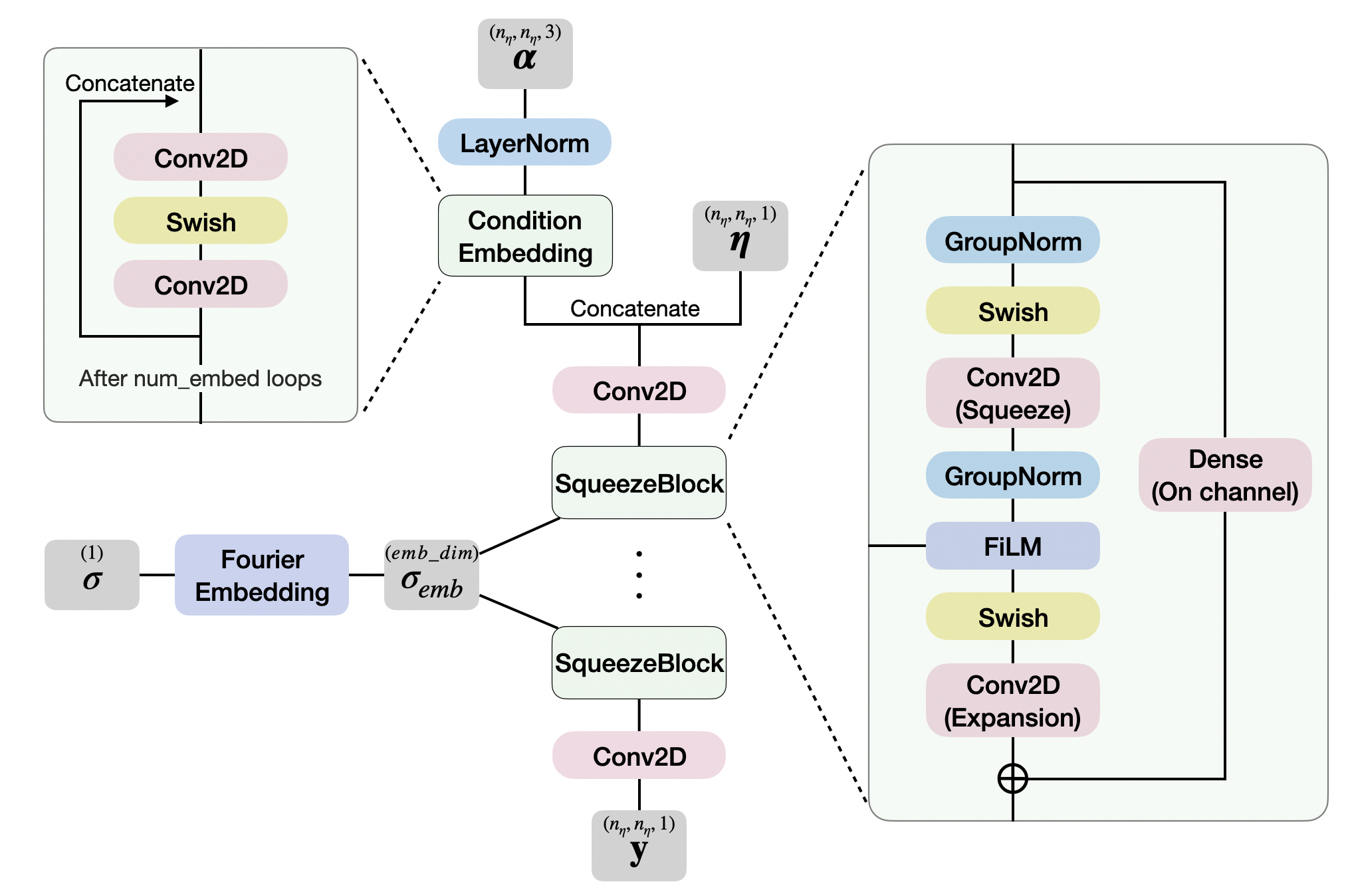
Figure 3: An overview of the architecture of the CNN-based representation.

Remark 4.5.

Other choices are available too, and they will be used in numerical section for comparison:

• U-Net Vision Transformer (U-ViT): The U-ViT architecture [106] follows a U-Net structure with a downsampling path to encode the input image into feature maps, and an upsampling path to decode these feature maps back to the original spatial dimensions. The attention mechanisms enhances its ability to capture long-range dependencies. We use the implementation in a public repository  and provide a summarized skeleton of the algorithm in 6. We note that the ConvBlock in the algorithm is a special case of the SqueezeBlock, where the parameters out_channels and squeeze_channels are set to be equal, PositionEmbedding adds a trainable 2D position embeddings, and AttentionBlock uses a multi-head dot product attention coupled with a residual connection.

4.3 The Flowchart of the Training with Preconditioning

The previous two sections have pinned the specific architectures to numerically conduct the back-scattering and the filtering processes. These choices will now be integrated to the training to learn the score function, as outlined below.

Recall from Sections 3.3-3.4 that the denoiser is identified through the optimization formulation. Adapting this process to our context, we define the objective functional:

$$\mathcal{L}(D):D(\bm{\eta},{\sf\Lambda},\sigma)\to\mathbb{R}$$ (64)

using

$$\mathcal{L}(D)=\mathbb{E}_{\sigma\sim p_{\text{train}}}\mathbb{E}_{(\bm{\eta},{\sf\Lambda})\sim p_{\text{data}}}\mathbb{E}_{\bm{n}\sim\mathcal{N}(\,\cdot\,;\bm{0},\sigma^{2}I)}\left[\lambda(\sigma)\left\|D_{\bm{\Theta}}(\bm{\eta}+\bm{n},{\sf\Lambda},\sigma)-\bm{\eta}\right\|^{2}_{2}\right]\,,$$ (65)

for a given noise level distribution $\sigma\sim p_{\text{train}}$ and a weight $\lambda(\sigma)$.

To conduct the minimization, we restrict ourselves to the feasible set of function space spanned by neural networks of the following form

$$\mathcal{A}=\{D_{\bm{\Theta}}:\Theta =\Theta_{1}\bigcup\Theta_{2}\,,\text{with}$$ (66)

$$D_{\bm{\Theta}}(\bm{\eta},{\sf\Lambda},\sigma)=c_{\text{skip}}(\sigma)\bm{\eta}+c_{\text{out}}(\sigma)S_{\bm{\Theta}_{2}}\left(c_{\text{in}}(\sigma)\bm{\eta},F_{\bm{\Theta}_{1}}({\sf\Lambda}),c_{\text{noise}}(\sigma)\sigma\right)\}\,,$$

where $c_{\text{skip}},c_{\text{out}},c_{\text{in}}$, and $c_{\text{noise}}$ are predefined coefficients, termed as preconditioning of the network. $F_{\bm{\Theta}_{1}}$ represents the back-scattering component of the inversion, and either EquiNet or B-EquiNet will be deployed to code $F_{\bm{\Theta}_{1}}$, as was done in (55). Similarly, CNN-based representation will be used for $S_{\bm{\Theta}_{2}}$. This guarantees $S_{\bm{\Theta}_{2}}(\bm{\eta},\bm{\alpha},\sigma)$ satisfies translational equivariance:

$$T_{\bm{a}}S_{\bm{\Theta}_{2}}(\bm{\eta},\bm{\alpha},\sigma)=S_{\bm{\Theta}_{2}}(T_{\bm{a}}\bm{\eta},T_{\bm{a}}\bm{\alpha},\sigma)\text{\quad for all $\bm{a}\in\mathbb{N}_{\eta}^{2}$}\,.$$ (67)

This choice of $S_{\bm{\Theta}_{2}}$ automatically guarantees that all functions in the feasible set (66) satisfy the translational equivariance for the denoiser, and as a consequence, the approximation to the score-function, see (48), is also translational equivarient, as required by Theorem 4.4. The whole NN architecture used to represent $D_{\bm{\Theta}}(\bm{\eta},{\sf\Lambda},\sigma)$ is summarized in Algorithm 1:

Algorithm 1 Neural Architecture of the Denoiser

1:procedure $D_{\bm{\Theta}}$($\bm{\eta},{\sf\Lambda},\sigma$)

2:     $\bm{\alpha}\leftarrow F_{\bm{\Theta}_{1}}(\sf\Lambda)$

3:     $\bm{s}\leftarrow S_{\bm{\Theta}_{2}}\left(c_{\text{in}}(\sigma)\bm{\eta},\bm{\alpha},c_{\text{noise}}(\sigma)\sigma\right)$

4:     return $c_{\text{skip}}(\sigma)\bm{\eta}+c_{\text{out}}(\sigma)\bm{s}$

5:end procedure

5 Numerical Examples

The architecture for our back-projection diffusion model is factorized into two neural networks applied in tandem: $F_{\bm{\Theta}_{1}}$ and $S_{\bm{\Theta}_{2}}$. This motivates us to name the models by joining the names of each component. Our main models are called EquiNet-CNN and B-EquiNet-CNN, where the latent intermediate field representation $\bm{\alpha}_{\sf\Lambda}\approx F_{\bm{\Theta}_{1}}({\sf\Lambda})$ is instantiated by EquiNet and B-EquiNet models (discussed in Section 4.1), and $S_{\bm{\Theta}_{2}}$ is instantiated by a CNN-based representation (introduced in Section 4.2.2).

The present the training/optimization formulation in Section 5.2, and we introduce the evaluation metrics in Section 5.3. We provide details on the datasets that are used for training in Section 5.4. In Section 5.5 we introduce the state-of-art ML-based deterministic and classical methods that we use as baselines to benchmark our methodology.

We perform an extensive suite of benchmarks to demonstrate the properties of our framework as mentioned in the introduction. In what follows we summarize each of the benchmarks.

Performance Comparison (Section 5.6): We show that EquiNet-CNN and B-EquiNet-CNN considerably outperform other state-of-the-art deterministic methods and classical methods on the three synthetic datasets.

Parameter Efficiency and Performance across Resolutions (Section 5.7): We demonstrate that the number of trainable parameters in EquiNet-CNN and B-EquiNet-CNN scales favorably with increasing resolution (and number of unknowns to reconstruct), showcasing their parameter efficiency, which refers to the ability of a model to achieve high performance with a relatively small number of parameters. EquiNet-CNN achieves high reconstruction accuracy, even for a challenging MRI Brain dataset ( [47, 48]). We show that the quality of reconstruction increases as the resolution of the training data (and the probing frequency) increases, resulting in images with more fine-grained details.

Sample Complexity (Section 5.8): We highlight the low-sample complexity of EquiNet-CNN by training the model with different training dataset with increasing number of samples. Remarkably, when trained on only 2000 data points, it achieves higher accuracy on a dataset with strong multiple back-scattering than the deterministic baselines.

Posterior Distribution (Section 5.9): We demonstrate that EquiNet-CNN captures the posterior distribution well, with the Relative Root Mean Square Error (RRMSE) between ground truth data and data sampled from the far-field patterns showing that the modes of the error distribution align with manual pixel-level adjustments of scatterers.

Cycle Skipping (Section 5.10): We showcase the stability of EquiNet-CNN by training it using only data at the highest frequency. We demonstrate that the cycle skipping phenomenon that often affects classical methods is noticeably mitigated by EquiNet-CNN.

Ablation Study (Section 5.11): We present an ablation study using different combinations of back-scattering architectures and representations for the physics-aware score function. EquiNet-CNN and B-EquiNet-CNN demonstrate a lower number of parameters while outperforming the variants based on the prescribed metrics.

Inverse Crime and Noisy Inputs (Section 5.12): We demonstrate the robustness of EquiNet-CNN against noise and varying levels of epistemic uncertainty in data. To avoid the infamous inverse crime we show that our methods produces high-quality reconstruction even when the input data was generated using solvers with different stencils, and when stochastic noise was added to it.

Mixed Dataset and Generalization (Section 5.13): When trained with all three synthetic datasets mixed together, we show that EquiNet-CNN can generate samples for each dataset with high accuracy, significantly outperforming other baseline deterministic models. We also evaluate the performance of EquiNet-CNN on out-of-distribution datasets, where the class of scatterers in the dataset is not present in the within-distribution training dataset.

5.1 Software and Hardware Stack

The wideband scattering data were generated using Matlab. Specifically, it was generated at frequencies of 2.5, 5, and 10 with a dimension of $n_{\mathrm{sc}}=80$. It took approximately 8 hours to generate the data on a server equipped with two Xeon E5-2698 v3 processors (totaling 32 cores and 64 threads) and 256 GB of RAM.

The models presented in this paper were implemented using JAX [107] and Flax [108], as well as the swirl-dynamics library  for the ML-pipeline [109]. The experiments were performed on two PNY NVIDIA Quadro RTX 6000 graphics cards.

5.2 Problem Formulation and Optimization

Following the notation introduced in Section 4.3, we denote the set of wideband scattering data by $\{{\sf\Lambda}^{\omega}\}_{\omega\in\bar{\Omega}}$ by ${\sf\Lambda}$, and the discrete inverse map by $\mathcal{F}_{d}^{-1}$.

Back-projection diffusion models generate samples from $p(\bm{\eta}|{\sf\Lambda})$ by using the reverse-time SDE in (54), whereas deterministic models approximate the discrete inverse map $\mathcal{F}_{d}^{-1}$ by a neural network $\Phi_{\bm{\Theta}}$ where $\bm{\Theta}$ denotes the trainable parameters of the deterministic network; namely they reconstruct perturbations by $\bm{\eta}\approx\Phi_{\bm{\Theta}}({\sf\Lambda})$.

The training dataset is identical for both deterministic and diffusion models and it consists of 21,000 data pairs of perturbation and scattering data $(\bm{\eta}^{[s]},{\sf\Lambda}^{[s]})$ following different distributions, where $[s]$ is the sample index. The evaluation is performed using testing datasets with 500 data points each, which have not been seen by the models during the training stage.

The following paragraphs cover training and sampling specifics of the denoiser $D_{\bm{\Theta}}$ introduced in Section 4.3.

Preconditioning

We train a conditional denoiser following the form:

$$D_{\bm{\Theta}}(\bm{\eta},{\sf\Lambda},\sigma)=c_{\text{skip}}(\sigma)\bm{\eta}+c_{\text{out}}(\sigma)S_{\bm{\Theta}_{2}}\left(c_{\text{in}}(\sigma)\bm{\eta},F_{\bm{\Theta}_{1}}(\sf\Lambda),c_{\text{noise}}(\sigma)\sigma\right)\,.$$ (68)

For the choices of preconditioning, we employ the formulas used in [93]. Specifically, they are

$$\left\{\begin{aligned} \text{Skip scaling}&\quad c_{\text{skip}}(\sigma)=\frac{\sigma^{2}_{\text{data}}}{\left(\sigma^{2}+\sigma^{2}_{\text{data}}\right)}\,,\\ \text{Output scaling}&\quad c_{\text{out}}(\sigma)=\frac{\sigma\cdot\sigma_{\text{data}}}{\sqrt{\sigma^{2}_{\text{data}}+\sigma^{2}}}\,,\\ \text{Input scaling}&\quad c_{\text{in}}(\sigma)=\frac{1}{\sqrt{\sigma^{2}+\sigma^{2}_{\text{data}}}}\,,\\ \text{Noise cond.}&\quad c_{\text{noise}}(\sigma)=\frac{1}{4}\ln(\sigma)\,,\end{aligned}\right.$$ (69)

where $\sigma_{\text{data}}$ is the standard deviation of the perturbations in the training dataset.

Training

The denoiser is trained to minimize the expected $L_{2}$ denoising error at samples drawn from $p_{\text{data}}$ for each noise level $\sigma\sim p_{\text{train}}$

$$\mathbb{E}_{\sigma\sim p_{\text{train}}}\mathbb{E}_{(\bm{\eta},{\sf\Lambda})\sim p_{\text{data}}}\mathbb{E}_{\bm{n}\sim\mathcal{N}(\,\cdot\,;0,\sigma^{2}I)}\left[\lambda(\sigma)\left\|D_{\bm{\Theta}}(\bm{\eta}+\bm{n},{\sf\Lambda},\sigma)-\bm{\eta}\right\|^{2}_{2}\right]\,,$$ (70)

where noise levels has distribution $\sigma\sim p_{\text{train}}$ and weighted by $\lambda(\sigma)$.

In our setting, we employ the loss weighting introduced in [93]

$$\lambda(\sigma)=\frac{\sigma^{2}+\sigma_{\text{data}}^{2}}{(\sigma\cdot\sigma_{\text{data}})^{2}}\,.$$ (71)

For the training noise sampling from $p_{\text{train}}$, we consider a function $\sigma_{\text{train}}(t)$ that is derived from a section of the tangent function $\tan(t)$. This section is linearly rescaled so that the input domain is $[0,1]$ and the output range is $[0,\sigma_{\text{max}}]$. We then sample noise from a uniform distribution in $t\in[t_{\sigma_{\text{min}}},1]$ such that $\sigma_{\text{train}}(t_{\sigma_{\text{min}}})=\sigma_{\text{min}}$.

Sampling

We generate samples using the reverse-time SDE:

$$d\bm{\eta}=\left[f(t)\bm{\eta}-g^{2}(t)\nabla_{\bm{\eta}}\log p_{t}(\bm{\eta}|\bm{\alpha}_{\sf\Lambda})\right]\,dt+g(t)\,dW_{t}\,.$$ (72)

However, it is advised in [93] that we formulate the SDE based on the scaling factor $s(t)$ and noise schedule $\sigma(t)$ defined in (36), which can be rewritten as

$$f(t)=\frac{\dot{s}(t)}{s(t)}\quad\text{and}\quad g(t)=s(t)\sqrt{2\dot{\sigma}(t)\sigma(t)}\,.$$ (73)

Substituting the formulas into the reverse-time SDE, we have

$$d\bm{\eta}=\left[\frac{\dot{s}(t)}{s(t)}\bm{\eta}-2s^{2}(t)\dot{\sigma}(t)\sigma(t)\nabla_{\bm{\eta}}\log p_{t}(\bm{\eta}|\bm{\alpha}_{\sf\Lambda})\right]\,dt+s(t)\sqrt{2\dot{\sigma}(t)\sigma(t)}\,dW_{t}\,.$$ (74)

In our experiments, we adopt the variance preserving formulation in [92], where

$$s^{2}(t)=\frac{\sigma^{2}_{\text{data}}}{\sigma^{2}_{\text{data}}+\sigma^{2}(t)}\,.$$ (75)

For solving the SDE, we consider a discretzation of time $t$ by a total of $N$ steps, i.e. $t_{n}=\frac{n}{N-1}$ for $n=0,1,\dots,N-1$, on which we employ an exponential decaying noise schedule:

$$\sigma(t_{n})=\sigma_{\text{max}}\left(\frac{\sigma_{\text{end}}}{\sigma_{\text{max}}}\right)^{t_{n}}\,.$$ (76)

The SDE is then solved by the Euler-Maruyama method [110].

Hyperparameters

In our experiments, we use normalized data, so we set $\sigma_{\text{data}}=1$. For training noise sampling, we set $\sigma_{\text{min}}=10^{-4}$ and $\sigma_{\text{max}}=100$. For solving the SDE, we use a time step $N=256$ and $\sigma_{\text{end}}=10^{-3}$. We trained back-projection diffusion models for 100 epochs using the Adam optimizer with Optax’s warmup_cosine_decay [111] as our scheduler. The initial learning rate was set to $1\times 10^{-5}$, gradually increased to a peak of $1\times 10^{-3}$ over the first 5% of the training steps, and then decayed to $1\times 10^{-8}$ by the end of training. We also employed an exponential moving average (EMA) [112] of the model parameters with $\text{ema\_decay}=0.999$ to stabilize the training and improve performance.

The training specifics of the baseline deterministic models are detailed in Section 5.5. The performance of each model are assessed using different metrics described in Section 5.3 that measure the error in terms of individual samples, and at the distributional level.

5.3 Metrics

In this part we present the metrics that we used to measure the error of our results. For detailed description of the metrics see Appendix C

• Relative Root Mean Square Error (RRMSE): This metric quantifies the relative misfit between the generated samples and the ground truth for each element from the testing set. The average is then taken across the testing set.

• Sinkhorn Divergence (SD): An optimal transport-based metric, the Sinkhorn Divergence computes the distance between the ground truth’s distribution and the estimated distribution. It involves computing a reference distance between the training set and the testing set, which is then compared to the distance between the testing set and the generated samples.

• Mean Energy Log Ratio (MELR): This metric assesses the quality of our samples by measuring the log-ratio of the energy spectrum (via Fourier modes) between the generated samples and the ground truth.

• Continuous Ranked Probability Score (CRPS): Used to measure the accuracy of our probabilistic model, this metric computes the difference between the estimated probabilities and the actual outcomes in the ground truth.

5.4 Datasets

The datasets consist of pairs of perturbation and scattering data $(\bm{\eta},{\sf\Lambda})$ from different distributions. The perturbations are sampled randomly from a predetermined distribution, and their corresponding far-field patterns at three different frequencies, following a dyadic decomposition, are obtained by solving (4) numerically.

The physical domain for the perturbations and intermediate fields was $[-0.5,0.5]^{2}$ discretized with a equispaced grid of $80\times 80$ points. The different operators were discretized with a tensorized finite differences stencil of $8$-th order in each dimention, and the radiation boundary conditions was implemented using the perfectly matched layer (PML) [113] of order 2 and intensity 80. The sparse linear system was solved using a sparse LU factorization via UMFPACK [114]. The wideband data was sampled with monochromatic plane waves with frequencies of 2.5, 5, and 10, see Section 2, for which the effective wavelength is 8 points per wavelength (PPW). In particular, we use $n_{\mathrm{sc}}=80$ receivers and sources, where receivers geometry are aligned with the directions of sources, i.e. 80 equiangular directions.

In our experiments, we first evaluate the effectiveness of the models using 3 different categories of synthetic perturbations: Shepp-Logan, 3-5-10h Triangles, and 10h Overlapping Squares, which covers most of the challenges from inverse problems: strong reflections hiding internal structure, small scatterers with features below Nyquist-Sampling rate, scatterers exhibiting strong multiple back-scattering (i.e., waves bouncing back several times).

• Shepp-Logan: The well-known Shepp-Logan phantom, which was created in 1974 by Larry Shepp and Benjamin F. Logan to represent a human head [115]. The medium has a strong discontinuity modeling an uneven skull, which produced a strong reflection, which in return renders the recovery of the interior features challenging for classical methods. The perturbations are generated based on randomly chosen scalings, densities, positions, and orientations for the phantoms [116].

• 3-5-10h Triangles: Right triangles of side length $3$, $5$ and $10$ pixels, which are randomly located and oriented, and it is possible for them to overlap with each other. In this case we test the capacity of the algorithm to image consisting of small scatterers that are slightly below sub-Nyquist in size. The number of triangles is chosen randomly from 1 to 10.

• 10h Overlapping Squares: 20 overlapping squares of side length $10$ pixels.

Figure 4 showcases one example for each of the three category.

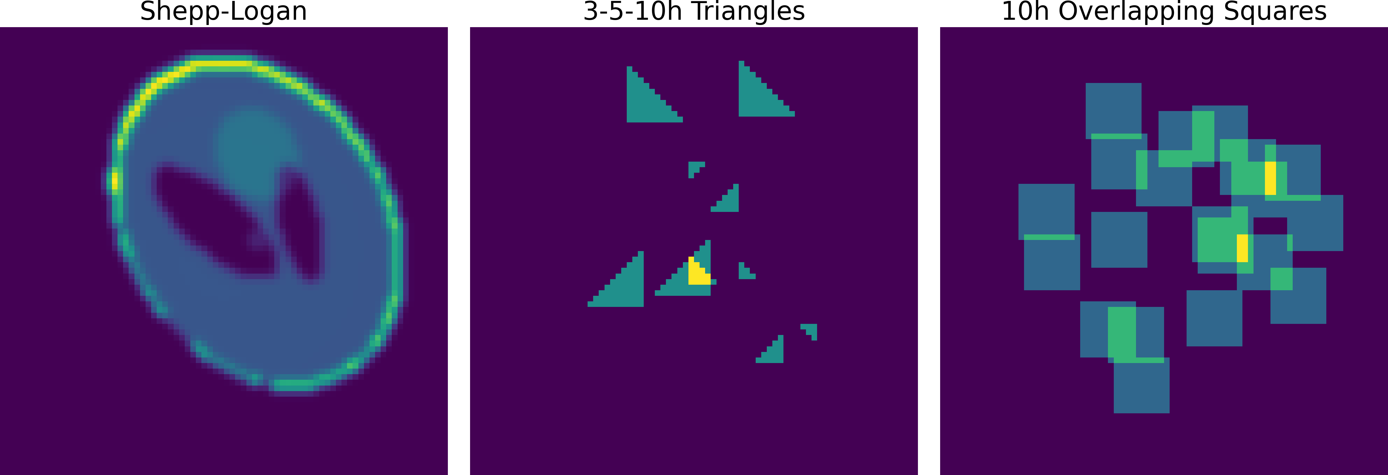
Figure 4: Examples of the three synthetic perturbations (Shepp-Logan, 3-5-10h Triangles, and 10h Overlapping Squares) used to benchmark the models.

In addition, we study the scaling of the number of trainable parameters and performance for different resolutions of EquiNet-CNN on the NYU fastMRI Brain data. The Brain MRI images used as our perturbations are obtained from the NYU fastMRI Initiative database [47]. We padded, resized, and normalized the perturbations to a native resolution at $n_{\eta}=240$ points representing the same physical domain $[-0.5,0.5]^{2}$. Then, we down-sampled the perturbations to resolutions $n_{\eta}=60,80,120$, and $160$. For the perturbations at resolution $n_{\eta}=60$, using the same method as introduced in the beginning of this section, we generated the far-field patterns discretized with $n_{\mathrm{sc}}=60$ at frequencies 3, 6, and 12, for which the effective wavelength is 5 PPW. For perturbation of different resolutions, we generated their far-field patterns with $n_{\mathrm{sc}}=n_{\eta}$ by sampling at proportionally scaled frequencies, which resulted in the same effective wavelength. More specifically, for resolutions at $n_{\eta}=80,120$ and $160$, we chose frequencies 4,8, and 16, frequencies 6,12, and 24, and frequencies 8,16, and 32 respectively.

Figure 5 showcases three examples of the Brain MRI perturbations at the native resolution $240\times 240$.

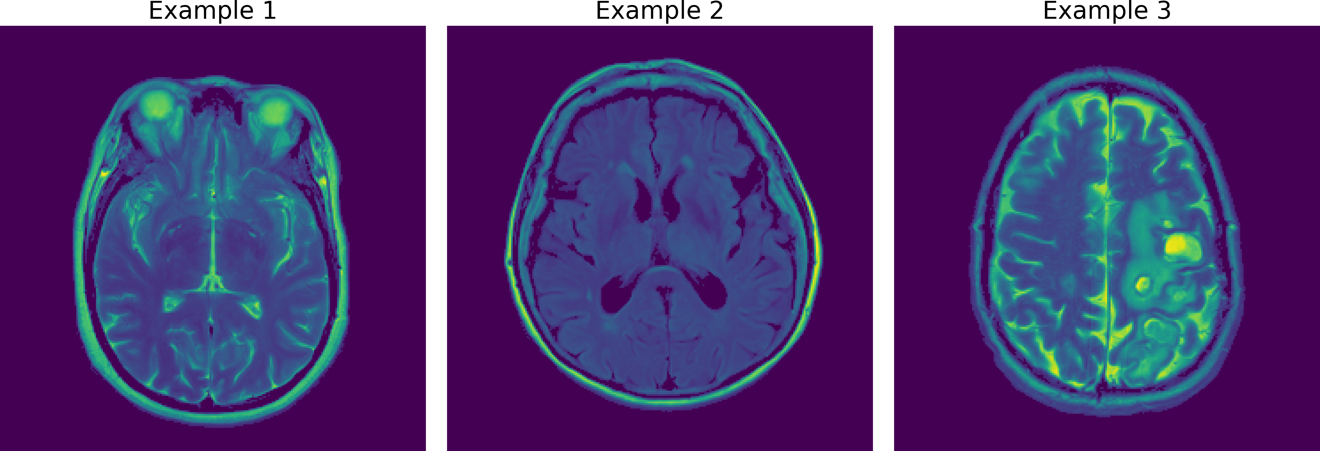
Figure 5: Examples of the Brain MRI perturbations.

5.5 Baselines

We use four state-of-the-art deterministic baselines when comparing our framework, which also leverage the filtered back-projection formula in (14), and they approximate the back-scattering operator and the filtering operator by neural networks. In particular, they all use a CNN to represent the filtering operator, respecting its translational equivariance, see Proposition 2.3. They differ primarily in their representations of the back-scattering operator. We briefly recap their features and detail the training specifics:

• SwitchNet [26] uses an incomplete Butterfly factorization to derive a low-complexity factorizaiton of the back-scattering operator, which is then replaced by a neural network.

• WideBNet [13] utilizes the butterfly factorization and Cooley-Tukey FFT algorithm to design its neural network.

• EquiNet [29] relies on a change of variable from the integral representation of the scattering operator to write a rotationally equivariant network.

• B-EquiNet [29] follows the same structure of EquiNet, but it relies on a Butterfly network to compress the operators.

For deterministic models, we decorate their model name with ‘(deterministic)’ and refer to them as EquiNet (deterministic), B-EquiNet (deterministic), WideBNet (deterministic) and SwitchNet (deterministic).

Optimization and Hyperparameters

The deterministic models are trained to minimize the mean square error between the network-produced perturbations and the ground truth perturbations (used to generate the input data), i.e.,

$$\min_{\bm{\Theta}}\frac{1}{N_{s}}\sum_{s=1}^{N_{s}}\|\Phi_{\bm{\Theta}}({\sf\Lambda}^{[s]})-\eta^{[s]}\|^{2}\,.$$ (77)

For training both SwitchNet (deterministic) and WideBNet (deterministic), the initial learning rate was set as $1\times 10^{-3}$ and the scheduler was set as Optax’s exponential_decay [111] with a decay rate of 0.95 after every 2000 transition steps with staircase set to true. Adam optimizer [117] is employed and we terminate training after 150 epochs. Additionally, we trained both EquiNet (deterministic) and B-EquiNet (deterministic) for 35 epochs using the Adam optimizer with Optax’s warmup_cosine_decay [111] as our scheduler. The initial learning rate was set to $1\times 10^{-5}$, gradually increased to a peak of $5\times 10^{-3}$ over the first 2000 steps, and then decayed to $1\times 10^{-7}$ by the end of training.

In addition to the ML-based approach we also considered PDE-constrained optimization approaches:

• Least Squares [118]: It uses the Born approximation to fix the background, it then finds the perturbation that minimizes the data misfit in (8) with respect to the fixed background. Additionally, in presence of the wideband data, it minimizes the sum of data misfits at all frequencies.

• Full Waveform Inversion (FWI) [2]: Similarly to the least-squares approach, it minimizes the same data misfit in (8), but it allows the background to be updated at each iteration. In presence of the wideband data, the optimization process the data hierarchically starting from the lowest frequency and slowly starting to process data at higher frequencies. We performed a sweep of different schedules with different combination of frequencies that provide the best reconstruction.

5.6 Performance Comparison

We compare reconstructions our three synthetic datasets (Shepp-Logan, 3-5-10h Triangles, and 10h Overlapping Squares) using our main models, EquiNet-CNN and B-EquiNet-CNN, alongside the baseline models introduced in Section 5.5. The models are benchmarked using the metrics RRMSE, MELR, and SD.

Table 1 summarizes the performance of each model on these datasets. It indicates that EquiNet-CNN and B-EquiNet-CNN considerably outperform other state-of-the-art deterministic methods and classical methods.

Model	RRMSE	MELR	SD
		$(\times 10^{-2})$
Shepp-Logan (Reference SD: 14.406)
EquiNet-CNN	1.414%	1.847	3.745
B-EquiNet-CNN	1.406%	1.757	3.754
EquiNet (deterministic)	1.693%	2.827	3.786
B-EquiNet (deterministic)	2.022%	2.906	3.831
WideBNet (deterministic)	3.843%	13.255	4.085
SwitchNet (deterministic)	4.305%	8.071	4.147
FWI	52.041%	241.893	8.893
Least Squares	154.645%	408.039	21.774
3-5-10h Triangles (Reference SD: 2.833)
EquiNet-CNN	1.590%	1.385	0.949
B-EquiNet-CNN	1.657%	1.318	0.952
EquiNet (deterministic)	2.741%	1.734	0.987
B-EquiNet (deterministic)	2.944%	2.010	0.990
WideBNet (deterministic)	17.263%	10.582	1.294
SwitchNet (deterministic)	15.084%	9.377	1.256
FWI	28.637%	159.894	1.501
Least Squares	41.666%	81.908	14.391
10h Overlapping Squares (Reference SD: 11.183)
EquiNet-CNN	1.744%	1.979	3.860
B-EquiNet-CNN	2.046%	2.683	3.894
EquiNet (deterministic)	10.891%	25.906	4.881
B-EquiNet (deterministic)	9.484%	21.434	4.727
WideBNet (deterministic)	14.327%	44.182	5.260
SwitchNet (deterministic)	20.102%	24.295	5.917
FWI	38.777%	281.057	7.948
Least Squares	163.037%	301.991	17.603

Table 1: Comparison of model performance on three synthetic datasets (Shepp-Logan, 3-5-10h Triangles, and 10h Overlapping Squares) using the metrics RRMSE, MELR, and SD. The table highlights the superior performance of EquiNet-CNN and B-EquiNet-CNN compared to various deterministic methods and classical approaches. The best performance metrics for each dataset are indicated in bold.

Additionally, Figures 6, 7, and 8 visually showcase model reconstructions on three synthetic datasets: Shepp-Logan, 10h Overlapping Squares, and 3-5-10h Triangles. These figures initially present plots of the ground truth and reconstructions. Notably, the reconstructions from Least Squares and Full Waveform Inversion have markedly lower quality than the other, prompting a further detailed comparison using region of interest (ROI) plots.

Figures 9, 10, and 11 focus on ROIs to highlight finer and more subtle differences between the reconstruction stemming from EquiNet-CNN, B-EquiNet-CNN, and the deterministic models. The first row of subplots presents the ROI of the ground truth alongside one ROI zoom-in. Subsequent rows display the ROI of reconstructions, ROI zoom-ins, Full Differences, and ROI Differences for each model. EquiNet-CNN and B-EquiNet-CNN exhibit considerably lower errors compared to other state-of-the-art deterministic models.

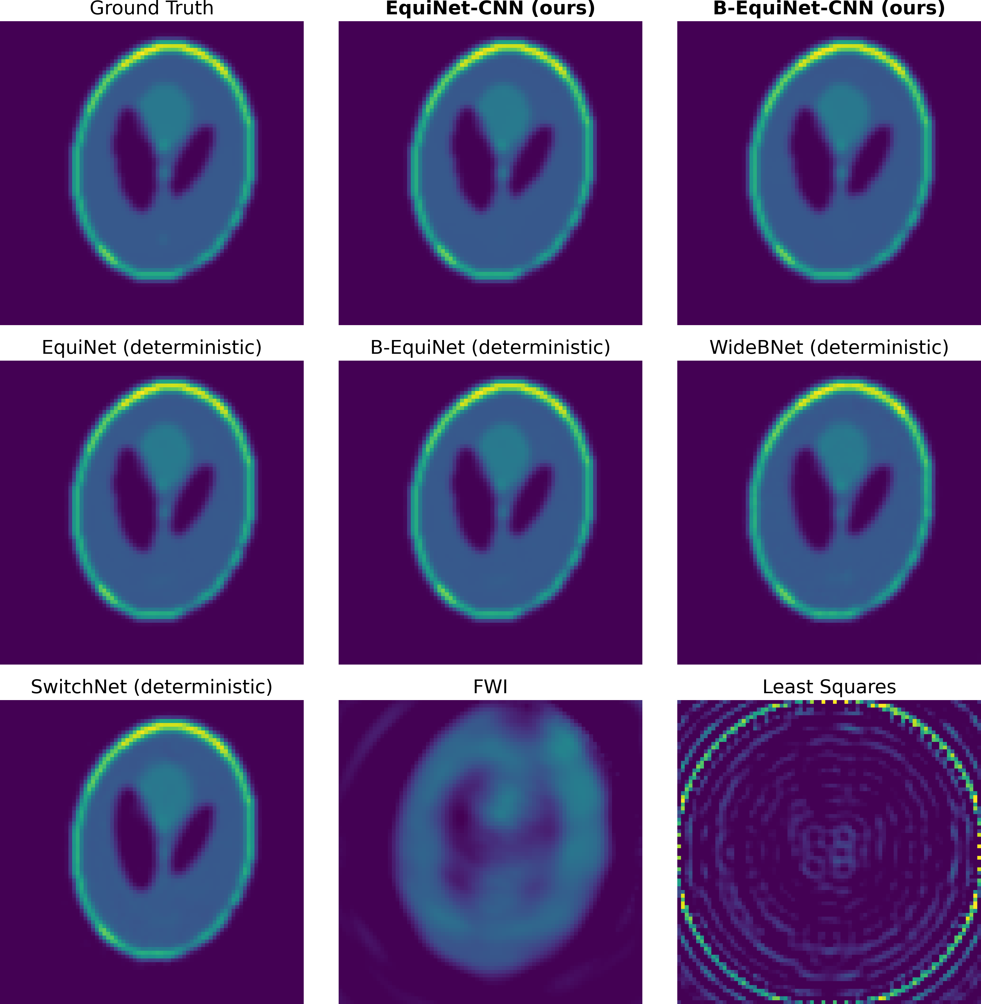
Figure 6: Model reconstructions from EquiNet-CNN, B-EquiNet-CNN, and baselines for the Shepp-Logan dataset. See Figure 9 for a detailed zoom-in comparison.

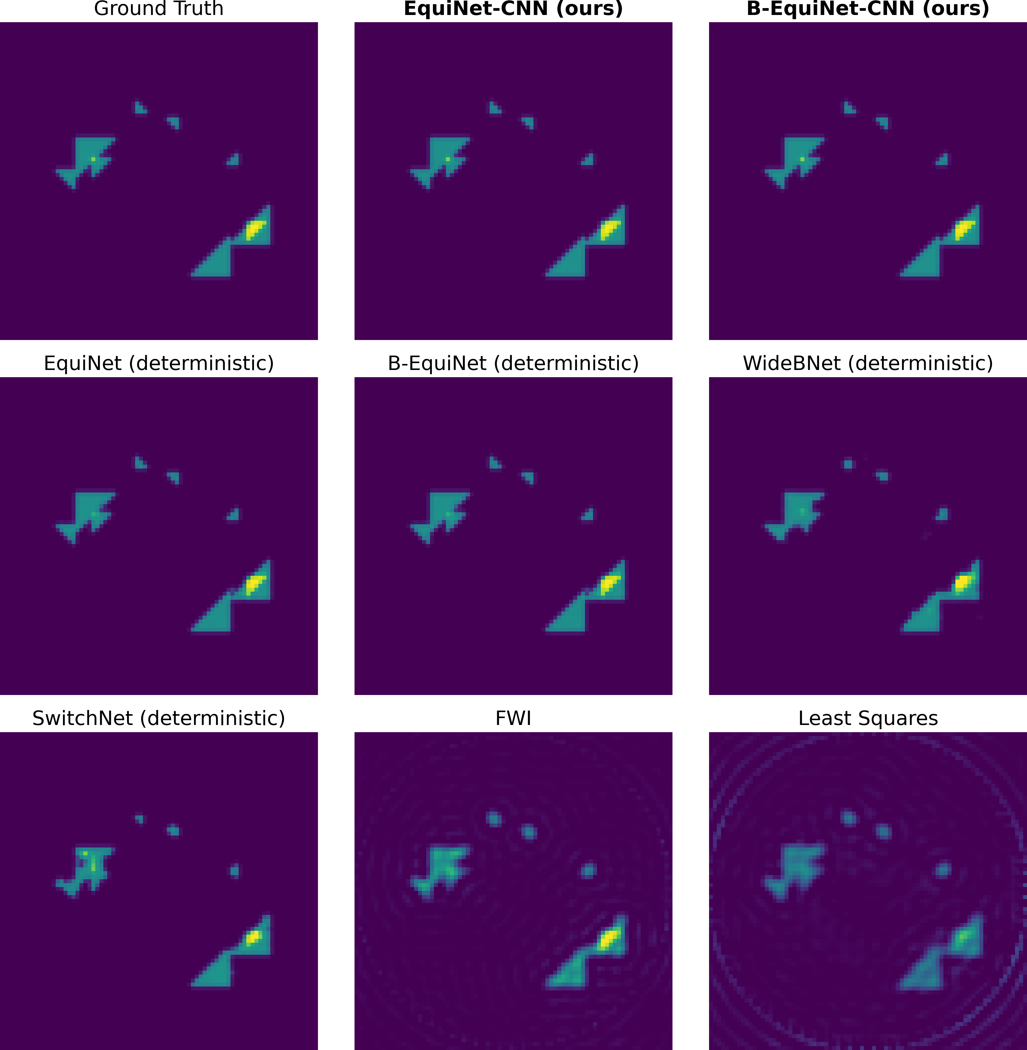
Figure 7: Model reconstructions from EquiNet-CNN, B-EquiNet-CNN, and baselines for the 3-5-10h Triangles dataset. See Figure 10 for a detailed zoom-in comparison.

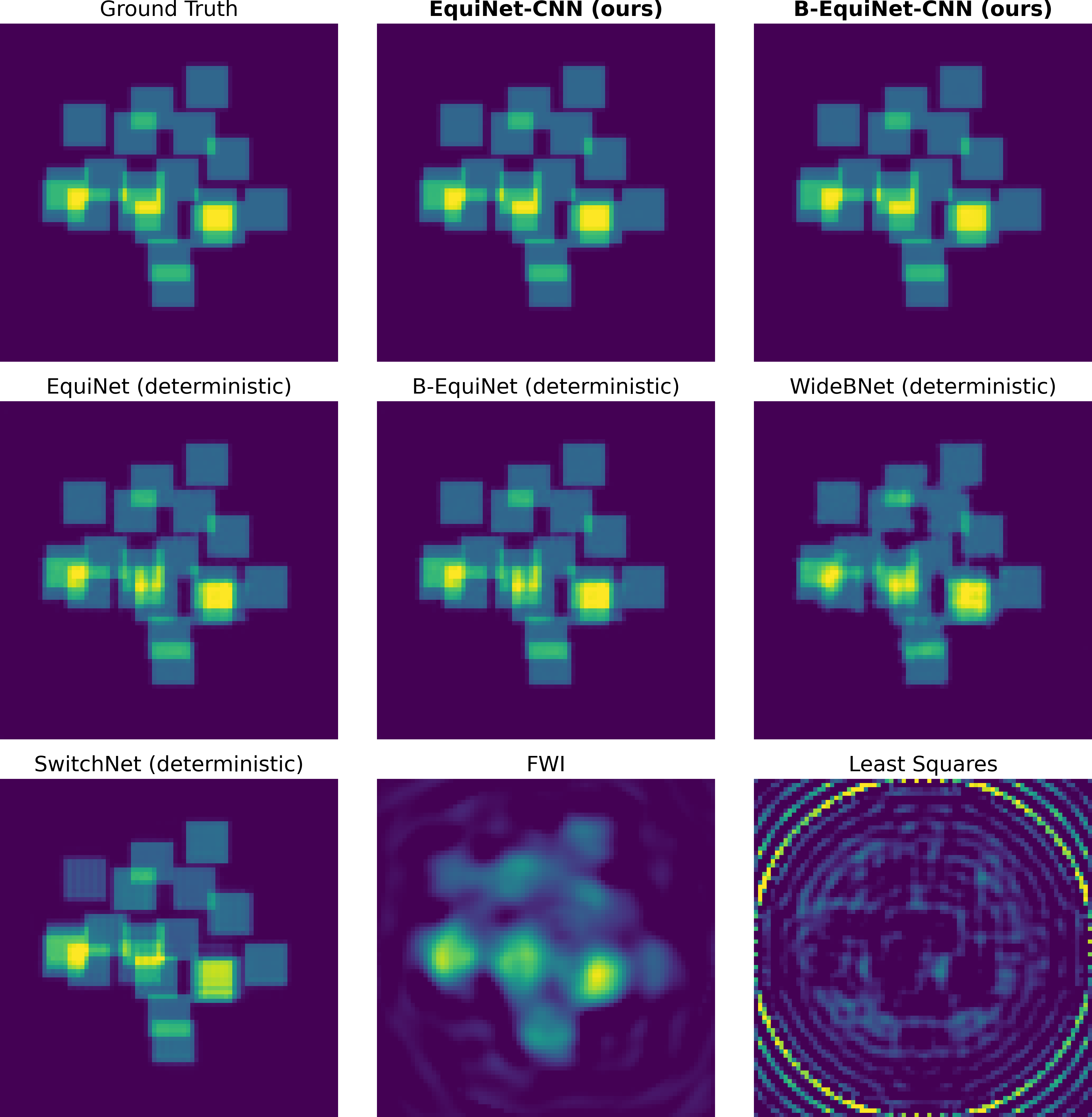
Figure 8: Model reconstructions from EquiNet-CNN, B-EquiNet-CNN, and baselines for the 10h Overlapping Squares dataset. See Figure 11 for a detailed zoom-in comparison.

Figure 9: Model reconstructions for the Shepp-Logan dataset, showcasing regions of interest (ROI), the detailed zoom-ins and differences for EquiNet-CNN, B-EquiNet-CNN, and baseline deterministic models.

Figure 10: Model reconstructions for the 3-5-10h Triangles dataset, showcasing regions of interest (ROI), the detailed zoom-ins and differences for EquiNet-CNN, B-EquiNet-CNN, and baseline deterministic models.

Figure 11: Model reconstructions for the 10h Overlapping Squares dataset, showcasing regions of interest (ROI), the detailed zoom-ins and differences for EquiNet-CNN, B-EquiNet-CNN, and baseline deterministic models.

5.7 Parameter Efficiency and Performance across Resolutions

In the design of EquiNet-CNN and the further compressed B-EquiNet-CNN, $S_{\bm{\Theta}_{2}}$ is a CNN-based representation that maintains a constant number of trainable parameters across all resolutions. Specifically, in our experiments, the CNN-based representation has 374,575 trainable parameters. Therefore, the asymptotic scaling of the number of trainable parameters in the models is entirely determined by $F_{\bm{\Theta}_{1}}$. The later is summarized in Table 2, and written relative to $N_{\text{unknown}}\mathrel{\mathop{:}}=n_{\eta}^{2}$, which is the number of grid points used in the reconstruction after the physical domain is discretized. In our experiments, we use a discretization of the same size for the scattering data, i.e., $N_{\text{unknown}}=n_{\eta}^{2}=n_{\mathrm{sc}}^{2}$ (see Section 2.3). Additionally, it should be noted that a fixed number of frequencies (in our case, three) are used to generate data at all resolutions.

Complexity	EquiNet-CNN	B-EquiNet-CNN
# Parameters	$\mathcal{O}(N_{\text{unknown}})$	$\mathcal{O}(\sqrt{N_{\text{unknown}}}\log{N_{\text{unknown}}})$

Table 2: Scaling of the number of trainable parameters with respect to the number of unknowns for B-EquiNet-CNN and EquiNet-CNN.

We test the performance of EquiNet-CNN on the MRI Brain datasets at resolutions $n_{\eta}=60,80,120,$ and $160$. Table 3 shows the numbers of trainable parameters of $F_{\bm{\Theta}_{1}}$ and $S_{\bm{\Theta}_{2}}$, denoted as $|\bm{\Theta}_{1}|$ and $|\bm{\Theta}_{2}|$ respectively, as well as the validation RRMSE at the training resolutions. In particular, Table 3 shows that the number of trainable parameters sublinearly with the total number of unknowns to reconstruct, demonstrating the model’s parameter efficiency. In addition, for the MRI Brain dataset, EquiNet-CNN achieves high accuracy in the reconstruction which further improves as the resolution of the data (and the frequency of the probing waves) increase.

Resolution ($n_{\eta}$)	$|\bm{\Theta}_{1}|$	$|\bm{\Theta}_{2}|$	RRMSE
60	87,840	374,575	5.363%
80	155,520	374,575	5.425%
120	348,480	374,575	5.062%
160	618,240	374,575	4.544%

Table 3: Number of trainable parameters and performance of EquiNet-CNN on MRI Brain datasets at different resolutions. Note that $|\bm{\Theta}_{2}|$ is a constant 374,575 at all resolutions and $|\bm{\Theta}_{1}|=\mathcal{O}(N_{\text{unknown}})$.

Figure 12 plots four different ground truth perturbations at resolutions $n_{\eta}=60,80,120$ and $160$ from the MRI Brain dataset, alongside their reconstructions using EquiNet-CNN. Even-numbered rows showcase ground truth images at native resolution 240 and its downsampled versions at 60, 80, 120, and 160 resolutions. The subsequent odd-numbered rows present corresponding reconstructions by EquiNet-CNN at these resolutions.

Figure 12: Ground truth perturbations and reconstructions from the MRI Brain dataset are displayed at resolutions 60, 80, 120, and 160. The rightmost column shows the ground truth perturbations at their native resolution of 240.

5.8 Sample Complexity

By exploiting the symmetries of the problem, specifically, the rotational equivariance of the back-scattering operator for the latent representation and the translational equivariance of the physics-aware score function, we significantly reduce the number of trainable parameters. With approximately half a million parameters, EquiNet-CNN demonstrates low sample complexity, as detailed in this section. We trained EquiNet-CNN on partial 10h Overlapping Squares datasets consisting of 1,000, 2,000, 4,000, 8,000, 16,000, and 21,000 data points for a fixed number of training steps at 131,250, which is equivalent to training for 100 epochs on 21,000 data points using a batch size of 16.

Table 4 shows the comparison of the reconstructions from the models using metrics such as RRMSE, MELR, SD, and CRPS. With only 2,000 data points for training, EquiNet-CNN already outperforms all baseline models trained on 21,000 data points. The accuracy stagnates when training with more than 8,000 data points. Figure 13 displays a typical reconstruction from each model on the 10h Overlapping Squares dataset. Note that for models trained with a small number of data points, the positions of the scatterers are not accurate.

Dataset Size	RRMSE	MELR	SD	CRPS
		$(\times 10^{-2})$		$(\times 10^{-4})$
10h Overlapping Squares (Reference SD: 11.183)
1,000	12.454%	12.041	5.080	28.953
2,000	7.893%	8.392	4.568	16.678
4,000	4.896%	5.464	4.224	8.469
8,000	2.756%	3.054	3.982	5.268
16,000	2.184%	2.375	3.915	4.404
21,000	1.744%	1.979	3.860	3.916

Table 4: Comparison of reconstructions of 10h Overlapping Squares from EquiNet-CNN models trained on partial 10h Overlapping Squares datasets of various sizes, using a fixed number of 131,250 training steps.

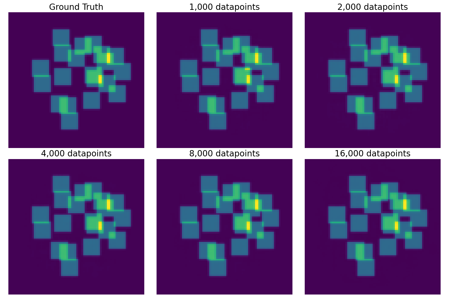
Figure 13: Comparison of reconstructions of 10h Overlapping Squares from EquiNet-CNN models using different dataset sizes. Notice that for models trained with a small number of data points, the position of the square scatterer in the middle is not accurate.

5.9 Posterior Distribution

Due to the probabilistic nature of the diffusion model, we test how well the EquiNet-CNN model captures the posterior distribution. Given that we do not have a ground truth for the posterior, we analyze the behavior of the reconstruction as we change the data used for training/inference. As such, we artificially increase uncertainty by training EquiNet-CNN with monochromatic data at frequencies: 2.5, 5, or 10 for the 10h Squares dataset, which due to the multiple back-scattering should be the most sensitive to partial data. Then we pick one data point one evaluation set, and we generate 500 conditional samples following $\bm{\eta}\sim p(\bm{\eta},{\sf\Lambda})$. Then for each of these samples we compute the data misfit as $\|\mathcal{F}^{\omega}(\eta)-\Lambda^{\omega}\|$ for each of the frequencies.

Table 5 shows the statistics of the data misfit at frequencies of 2.5, 5, and 10 and Figure 14 shows the estimated probability distributions of the data misfit for EquiNet-CNN trained on data at single a frequency of 2.5, 5, and 10, as well as at wideband frequencies including 2.5, 5, and 10. We can be observe from the distributions that there are several modes, which correspond to cases where some squares in the reconstruction are shifted by one or more pixels from the ground truth. As reference, Table 6 records the data misfit induced by manually moving a square in the ground truth by $n$ pixels; the errors match the locations of the modes in the distribution. As expected using single low-frequency data produces the biggest uncertainty, and the wide-band data produces the least.

Trained on Data at Frequency 2.5
Frequency	Mean (%)	Median (%)	Min (%)	Max (%)	Std (%)
2.5	4.083	4.036	1.342	9.087	1.243
5	4.486	4.452	1.248	9.045	1.105
10	7.877	7.934	1.844	14.721	1.801

Trained on Data at Frequency 5
Frequency	Mean (%)	Median (%)	Min (%)	Max (%)	Std (%)
2.5	1.851	1.637	0.744	5.636	0.825
5	1.658	1.455	0.665	4.886	0.736
10	2.532	2.214	1.008	7.431	1.148

Trained on Data at Frequency 10
Frequency	Mean (%)	Median (%)	Min (%)	Max (%)	Std (%)
2.5	2.664	2.397	0.663	9.269	1.506
5	2.369	2.144	0.662	8.151	1.327
10	3.613	3.258	1.005	12.418	2.023

Trained on Data at Wideband Frequencies including 2.5, 5, and 10
Frequency	Mean (%)	Median (%)	Min (%)	Max (%)	Std (%)
2.5	1.425	1.260	0.308	5.159	0.824
5	1.265	1.097	0.307	4.521	0.719
10	1.918	1.656	0.473	6.859	1.092

Table 5: Statistics of data misfit at different frequencies for 500 samples generated using EquiNet-CNN on 1 data point from the 10h Overlapping Squares dataset.

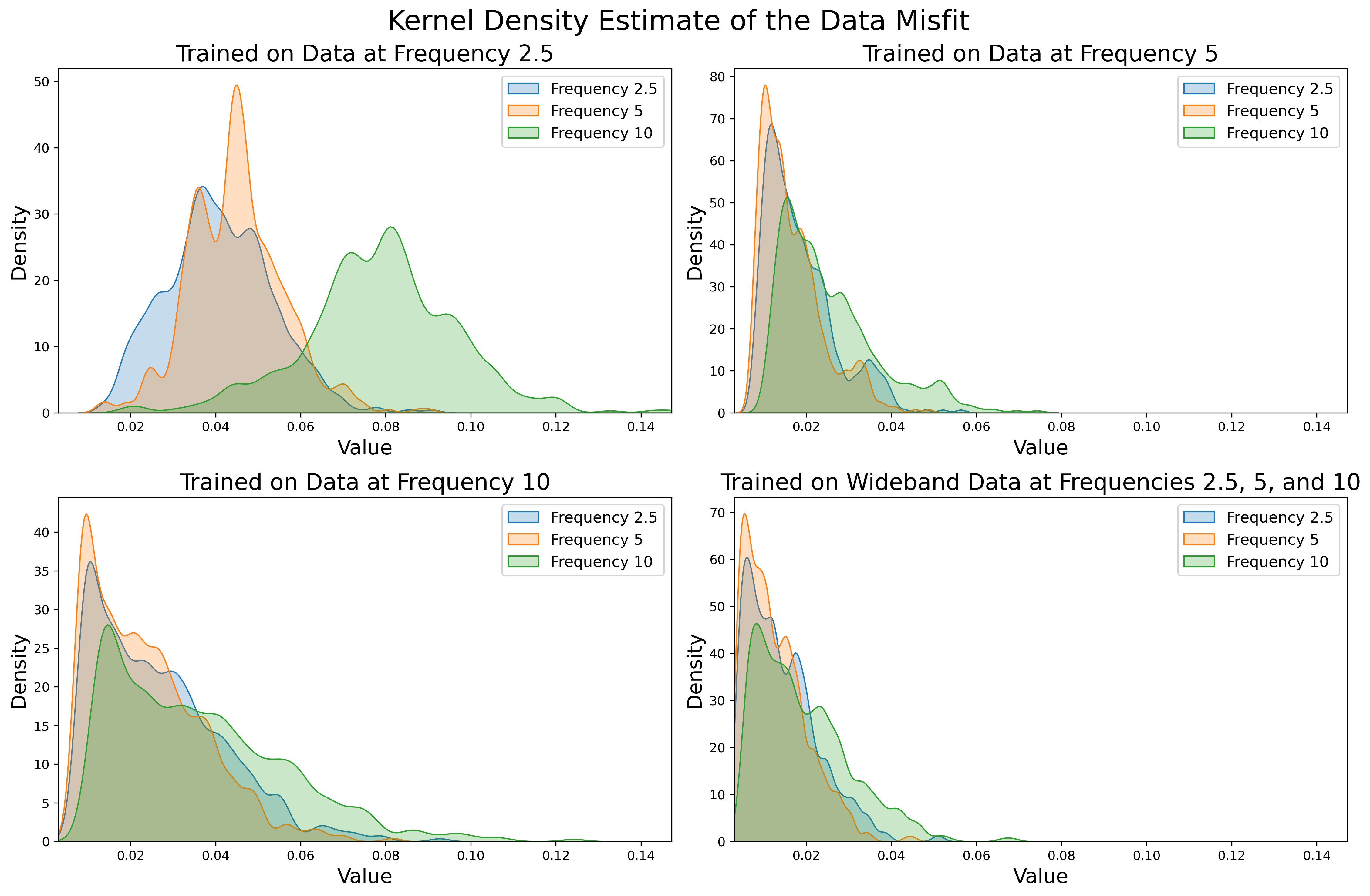
Figure 14: Estimated distributions of the data misfit for EquiNet-CNN, trained on data at a single frequency of 2.5, 5, and 10, as well as at wideband frequencies including 2.5, 5, and 10.

Pixels$\backslash$Frequency	2.5	5	10
1	3.265%	3.213%	5.214%
2	6.484%	6.340%	9.610%
3	9.603%	9.050%	12.931%
4	12.513%	11.401%	15.790%
5	15.202%	13.446%	18.501%

Table 6: data misfit in magnitude induced by manually moving a square in the ground truth by $n$ pixels.

5.10 Cycle Skipping

When training with only high-frequency data, classical methods like WI often encounter a phenomenon known as cycle skipping, where the algorithm converges to a local minimum. We demonstrate that the EquiNet-CNN model significantly mitigates cycle skipping. As such, we trained the model on the Shepp-Logan, 3-5-10h Triangles, and 10h Overlapping Squares datasets using data only at a high frequency of 10. Table 7 shows the metrics, RRMSE, MELR, SD, and CRPS of the reconstructions. From table 7 we can observe that for the Shepp-Logan and 3-5-10h Triangles, training with data only at a frequency of 10, the model yields results comparable to those obtained with wideband data. As expected from the previous section, the reconstruction of 10h Overlapping squares deteriorates when using only high-frequency data, due to the stronger back-scattering, although, the error remains relatively small.

	Shepp-Logan		3-5-10h Triangles		10h Overlapping Squares
Metric $\backslash$ Frequency	2.5-5-10	10	2.5-5-10	10	2.5-5-10	10
RRMSE	1.414%	1.738%	1.590%	1.955%	1.744%	4.993%
MELR ($\times 10^{-2}$)	1.847	2.045	1.385	1.969	1.979	4.603
SD	3.745	3.792	0.949	0.955	3.860	4.242
CRPS ($\times 10^{-4}$)	5.550	8.287	0.812	1.135	3.916	13.335

Table 7: RRMSE, MELR, SD, and CRPS of reconstructions from EquiNet-CNN trained using wideband data at frequencies of 2.5, 5, and 10, or using data at a frequency of 10.

Figure 15 plots the reconstructions from EquiNet-CNN trained with either wideband data or data at the highest frequency. In both cases, the errors are not noticeable to the naked eye.

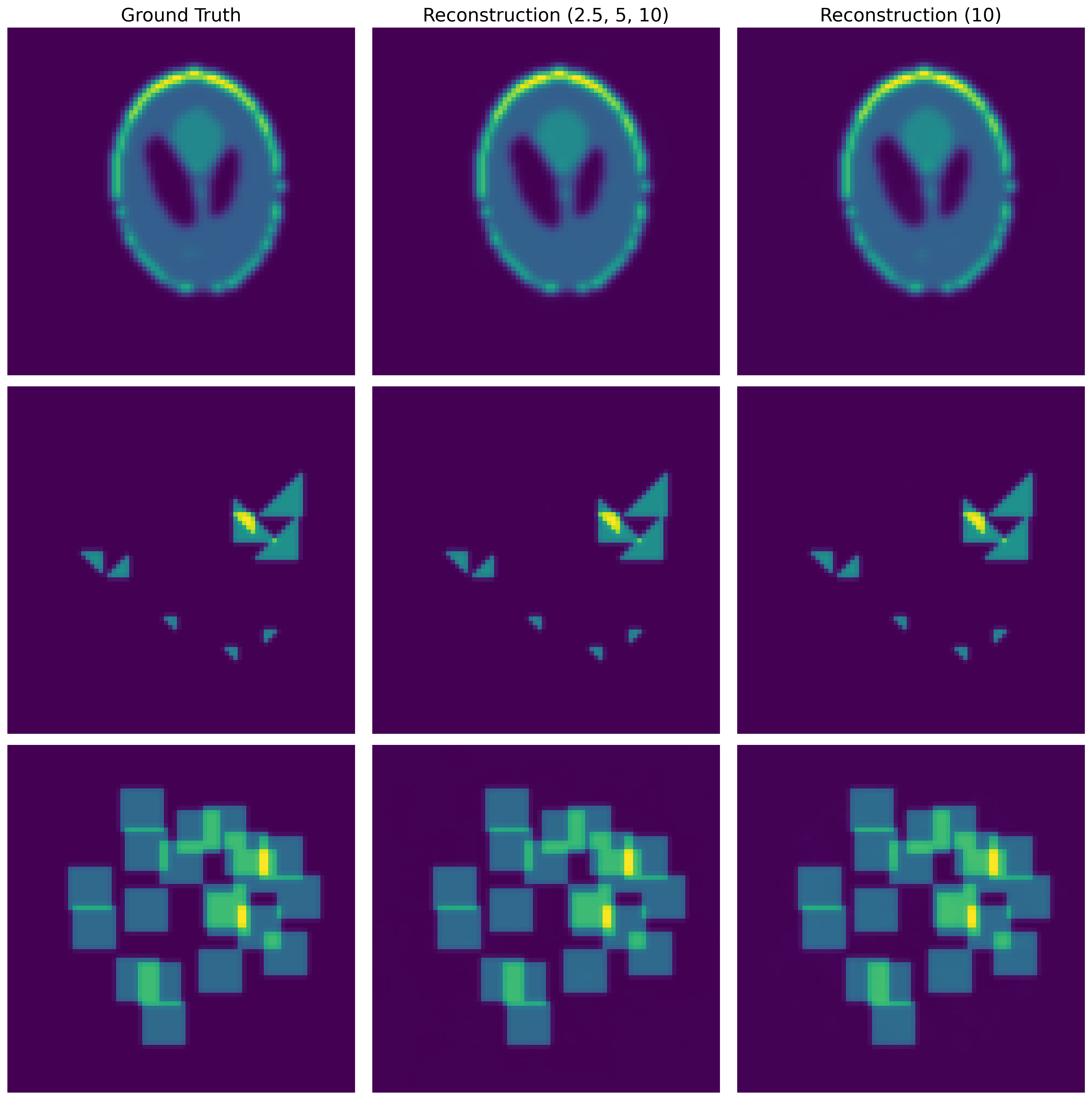
Figure 15: Comparison of reconstructions from the EquiNet-CNN trained with either wideband data at frequencies of 2.5, 5, and 10, or data at the highest frequency of 10.

5.11 Ablation Studies

Our main method relies on computing a latent representation of the intermediate field before using it to perform conditional sampling, where this latent representation is a neural network whose architecture is inspired by the back-scattering operators, see (16), which in return mimics the physics of wave propagation.

We show that this step is crucial for the behavior of our algorithm, thus we consider a few variants of our main model EquiNet-CNN and B-EquiNet-CNN, which modifies different parts of the algorithmic pipeline.

U-ViT Diffusion Model

we use regular state-of-the-art conditional diffusion model [93], to which we feed the discretized far-field patterns data directly. The neural architecture is a U-ViT network, see Remark 4.5. We refer to the model as None-U-ViT.

Back-Projection CNN Diffusion Models

In this class we find four models: B-EquiNet-CNN, SwitchNet-CNN, WideBNet-CNN, and Analytical-CNN. Similar to our main model EquiNet-CNN, the first three models preprocess the condition, i.e. the far-field patterns data, by using latent intermediate field representations of the corresponding deterministic models, whereas the Analytical-CNN use the analytical expression of the back-scattering operator $F^{\ast}$ in (16) to compute the latent intermediate field representation. Then, all of them use the CNN-based representation, introduced in Section 4.2.2, to represent the physic-aware score function.

Back-Projection U-ViT Diffusion Model

we use the latent representation stemming from EquiNet to represent the intermediate field, but use a U-ViT to represent the physics-aware score function, instead of the CNN-based networks used by the other models.

For each model we run a similar benchmark as the one in Section 5.6, whose results are are summarized in Table 8. Across the board our method outperforms the variants. We point out that, using the analytical expression is competitive for datasets that are simple, or that they don’t have complicated multiple back-scattering. EquiNet-U-ViT has comparable performance with EquiNet-CNN and B-EquiNet-CNN while having about 10 times more trainable parameters. We compare the number of trainable parameters recorded in Table 9, by which we observe the main advantage of using symmetries in the construction of the network, as the number of parameter is around an order of magniture lower for EquiNet-CNN and B-EquiNet-CNN while outperforming the rest of the networks. Also, EquiNet-CNN and B-EquiNet-CNN outperforms a pure U-ViT network, which underscores the advantages of the factorization introduced in this paper.

Model	RRMSE	MELR	SD	CRPS
		$(\times 10^{-2})$		$(\times 10^{-4})$
Shepp-Logan (Reference SD: 14.406)
EquiNet-CNN	1.414%	1.847	3.745	5.550
B-EquiNet-CNN	1.406%	1.757	3.754	5.318
WideBNet-CNN	5.271%	4.881	4.294	17.982
SwitchNet-CNN	1.943%	1.925	3.828	6.232
Analytical-CNN	2.371%	2.488	3.885	10.097
None-U-ViT	5.110%	3.097	4.256	9.474
EquiNet-U-ViT	1.663%	2.325	3.784	6.385
3-5-10h Triangles (Reference SD: 2.833)
EquiNet-CNN	1.590%	1.385	0.949	0.815
B-EquiNet-CNN	1.657%	1.318	0.952	0.821
WideBNet-CNN	17.197%	7.304	1.314	4.361
SwitchNet-CNN	8.033%	3.881	1.112	1.858
Analytical-CNN	6.434%	3.462	1.060	2.065
None-U-ViT	13.940%	5.868	1.246	2.315
EquiNet-U-ViT	2.454%	1.585	0.976	0.849
10h Overlapping Squares (Reference SD: 11.183)
EquiNet-CNN	1.744%	1.979	3.860	3.916
B-EquiNet-CNN	2.046%	2.683	3.894	5.298
WideBNet-CNN	18.010%	17.595	5.715	48.399
SwitchNet-CNN	10.644%	10.526	4.899	21.345
Analytical-CNN	11.946%	11.660	5.037	24.422
None-U-ViT	12.171%	12.191	5.060	16.425
EquiNet-U-ViT	2.035%	2.221	3.848	5.580

Table 8: Comparison of model performance on three synthetic datasets (Shepp-Logan, 3-5-10h Triangles, and 10h Overlapping Squares) using the metrics RRMSE, MELR, SD, and CRPS. The best performance metrics for each dataset are indicated in bold.

Model	Number of Trainable Parameters
EquiNet-CNN	530,095
B-EquiNet-CNN	434,479
WideBNet-CNN	2,287,025
SwitchNet-CNN	9,679,273
Analytical-CNN	378,793
None-U-ViT	5,746,445
EquiNet-U-ViT	5,753,351

Table 9: Number of trainable parameters for the models.

5.12 Inverse Crime and Noisy Inputs

In general the input data will have a certain amount of uncertainty either epistemic, due to an incomplete knowledge of the physical system, or stochastic, such as slight movement on the receivers.

Thus, we showcase the resilience of our method to small changes in the data distributions stemming from uncertainties on the physical models or stochastic noise in the inputs.

Using the same numerical method for generating the training data, and performing the reconstructing is usually called the inverse crime in the inverse problem community. In statistical terms this issue is related to overfitting the model to a particular distribution. To asses if our framework suffers from this issue we fed our trained models input data produced by a numerical solver using a different finite differences discretization, i.e., using a different stencil. Figure 16 plots the scattering data $\Lambda$ at frequency 10, and show the difference between $\Lambda$ generated using an 8th order stencil and 4th order stencil. In this case we can observe that there are differences in the amplitude of the largest reflections by around 5%, although, the plot does not show any large phase errors.

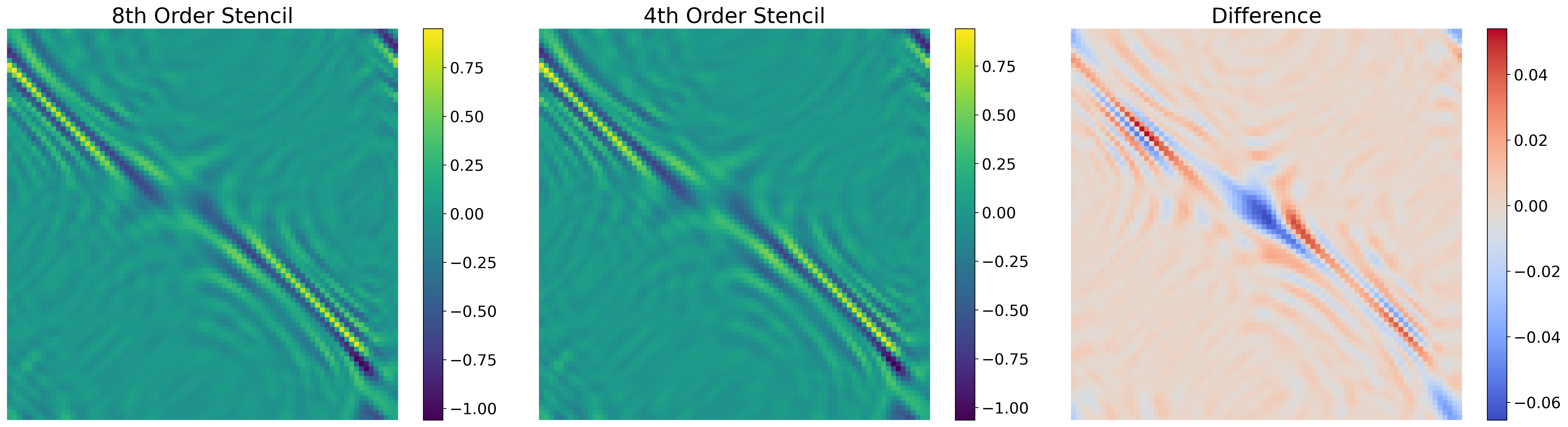
Figure 16: Comparison of the scattering data at a frequency of 10 using 8th and 4th order stencils, and the difference between them.

We point out, that due to dispersion errors, the differences become more apparent with fields at higher frequency.

Table 10 shows that the RRMSE of the reconstruction when using within-distribution and out-of-distribution input data, i.e., data generated with same stencil (order = 8) as the training data, and data using a different stencil (order 4 or 6). We can observe that across the different distribution of scatterers used in this work, the difference is minimal in the error. In summary, table 10 demonstrates that the model EquiNet-CNN is stable under moderate perturbation of the input distribution induced by using a different numerical solver.

Dataset/Stencil	4th Order Stencil	6th Order Stencil	8th Order Stencil
Shepp-Logan	1.581%	1.402%	1.414%
3-5-10h Triangles	1.537%	1.550%	1.590%
10h Overlapping Squares	1.788%	1.773%	1.744%

Table 10: RRMSE comparisons for EquiNet-CNN across different datasets and stencil orders, demonstrating the model’s stability with within-distribution and out-of-distribution inputs.

For the case of stochastic uncertainty, we feed our model with scattering data artificially corrupted by different noise levels. The data is corrupted using additive Gaussian noise following,

$${\sf\Lambda}_{\text{noised}}={\sf\Lambda}+\gamma_{\text{noise}}\sigma_{{\sf\Lambda}}\bm{\varepsilon}$$ (78)

where, $\bm{\varepsilon}$ follows a unit normal distribution, $\sigma_{{\sf\Lambda}}$ is the standard deviation of the scattering data, and $\gamma_{\text{noise}}$ is the noise level. Examples of these noised scattering data, ${\sf\Lambda}_{\text{noised}}$, are showcased in Figure 17. From the figure we can observe that the largest reflections and transmission waves are still legible, although for noise levels beyond 20%, i.e., $\gamma_{\text{noise}}=0.2$, most of the multiple back-scattered waves are drowned by the noise.

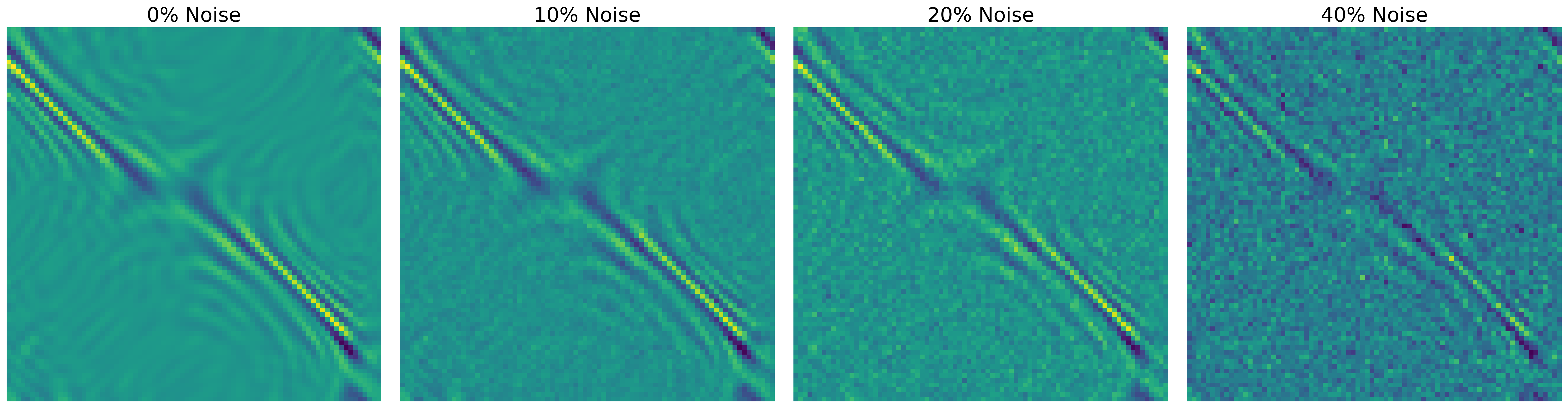
Figure 17: Comparison of data at a frequency of 10, noise-free, and with different levels of noise (10%, 20%, 40%). We can observe that beyond 20% noise, most of the waves stemming from multiple scattering reflections are drowned by the noise.

We perform a similar benchmark to the one presented in Section 5.6 but add noise at 4 different level (10%, 20%, and 40%) to the testing data for each of the three synthetic datasets, and we compare the RRMSE, MELR, SD, and CRPS of the resulting reconstructions. The results are summarized in Table 11, which shows how the reconstruction using EquiNet-CNN deteriorates as the noise increases. To provide visual cues on how the noise corrupts the recontruction we provide some samples of the reconstruction in Figure 18, which shows typical reconstruction at different levels of noise from the three synthetic datasets.

Noise Level	RRMSE	MELR	SD	CRPS
		$(\times 10^{-2})$		$(\times 10^{-4})$
Shepp-Logan (Reference SD: 14.406)
0% Noise	1.414%	1.847	3.745	5.550
10% Noise	3.355%	2.483	4.017	9.595
20% Noise	7.422%	4.344	4.576	30.890
40% Noise	14.827%	8.536	5.575	77.136
3-5-10h Triangles (Reference SD: 2.833)
0% Noise	1.590%	1.385	0.949	0.812
10% Noise	1.564%	1.161	0.949	0.768
20% Noise	1.618%	1.203	0.950	0.806
40% Noise	3.522%	2.053	0.977	1.474
10h Overlapping Squares (Reference SD: 11.183)
0% Noise	1.744%	1.979	3.860	3.916
10% Noise	2.675%	2.913	3.973	5.073
20% Noise	8.464%	8.426	4.627	15.114
40% Noise	24.761%	21.530	6.454	104.699

Table 11: Model performance of EquiNet-CNN on three synthetic datasets as noise levels increase from 10% to 40%. We evaluate using the metrics RRMSE, MELR, SD, and CRPS.

We can observe that even for relatively high-levels of noise the algorithm is still able to reconstruct the main features.

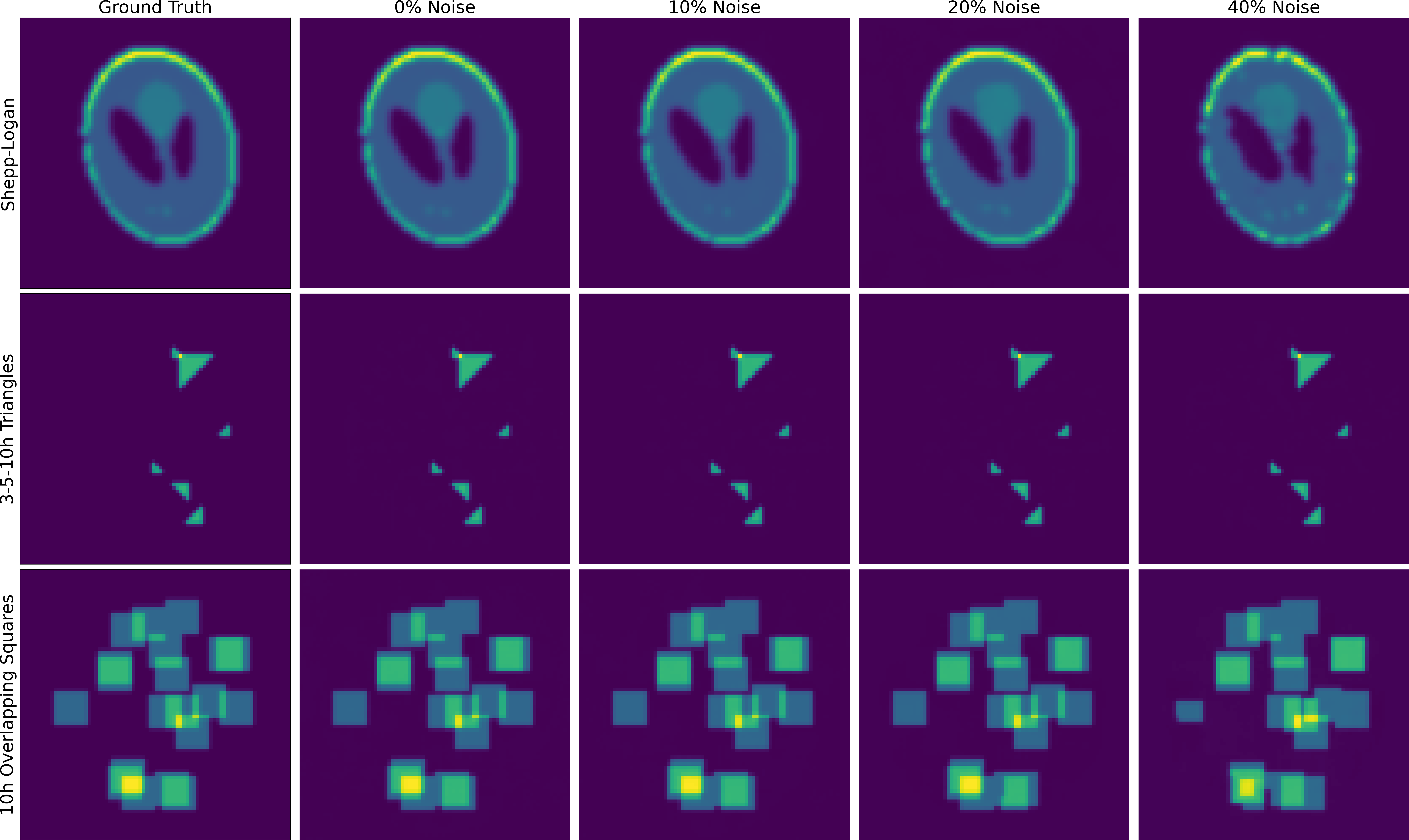
Figure 18: Comparison of reconstructions from EquiNet-CNN on the three synthetic datasets as noise increases from 0% to 40%.

To put these results in context, we perform the same procedure using some of the baselines, whose results are summarized in Table 12, which records the RRMSE of reconstructions between EquiNet-CNN and the deterministic models: EquiNet, B-EquiNet, WideBNet and SwitchNet. From this Table we can observe the our methodology has overall the lowest reconstruction error for all levels of noise. In addition, Figure 19 shows a typical reconstruction using EquiNet-CNN and baseline deterministic models for the Shepp-Logan dataset at different levels of noise. In this case we can observe that even though the error is large we can still observe many of the main features of the Shepp-Logan phantom.

Shepp-Logan
Model	0% Noise	10% Noise	20% Noise	40% Noise
EquiNet-CNN	1.414%	3.355%	7.422%	14.827%
EquiNet (deterministic)	1.693%	3.549%	7.512%	17.357%
B-EquiNet (deterministic)	2.022%	4.030%	7.801%	15.738%
WideBNet (deterministic)	3.843%	7.417%	13.227%	26.019%
SwitchNet (deterministic)	4.305%	6.173%	10.022%	21.111%
3-5-10h Triangles
Model	0% Noise	10% Noise	20% Noise	40% Noise
EquiNet-CNN	1.590%	1.564%	1.618%	3.522%
EquiNet (deterministic)	2.741%	4.143%	4.508%	5.623%
B-EquiNet (deterministic)	2.944%	4.028%	4.430%	7.596%
WideBNet (deterministic)	17.263%	19.632%	21.422%	30.021%
SwitchNet (deterministic)	15.084%	16.981%	18.859%	23.230%
10h Overlapping Squares
Model	0% Noise	10% Noise	20% Noise	40% Noise
EquiNet-CNN	1.744%	2.675%	8.464%	25.379%
EquiNet (deterministic)	10.891%	12.046%	15.653%	27.732%
B-EquiNet (deterministic)	9.484%	12.536%	20.129%	36.117%
WideBNet (deterministic)	14.327%	17.048%	23.730%	39.998%
SwitchNet (deterministic)	20.102%	22.217%	27.243%	40.178%

Table 12: Comparison of RRMSE of reconstructions for Shepp-Logan, 3-5-10h Triangles, and 10h Overlapping Squares datasets between EquiNet-CNN and deterministic models (EquiNet, B-EquiNet, WideBNet, and SwitchNet) at different noise levels. The best performance metrics for each dataset are indicated in bold.

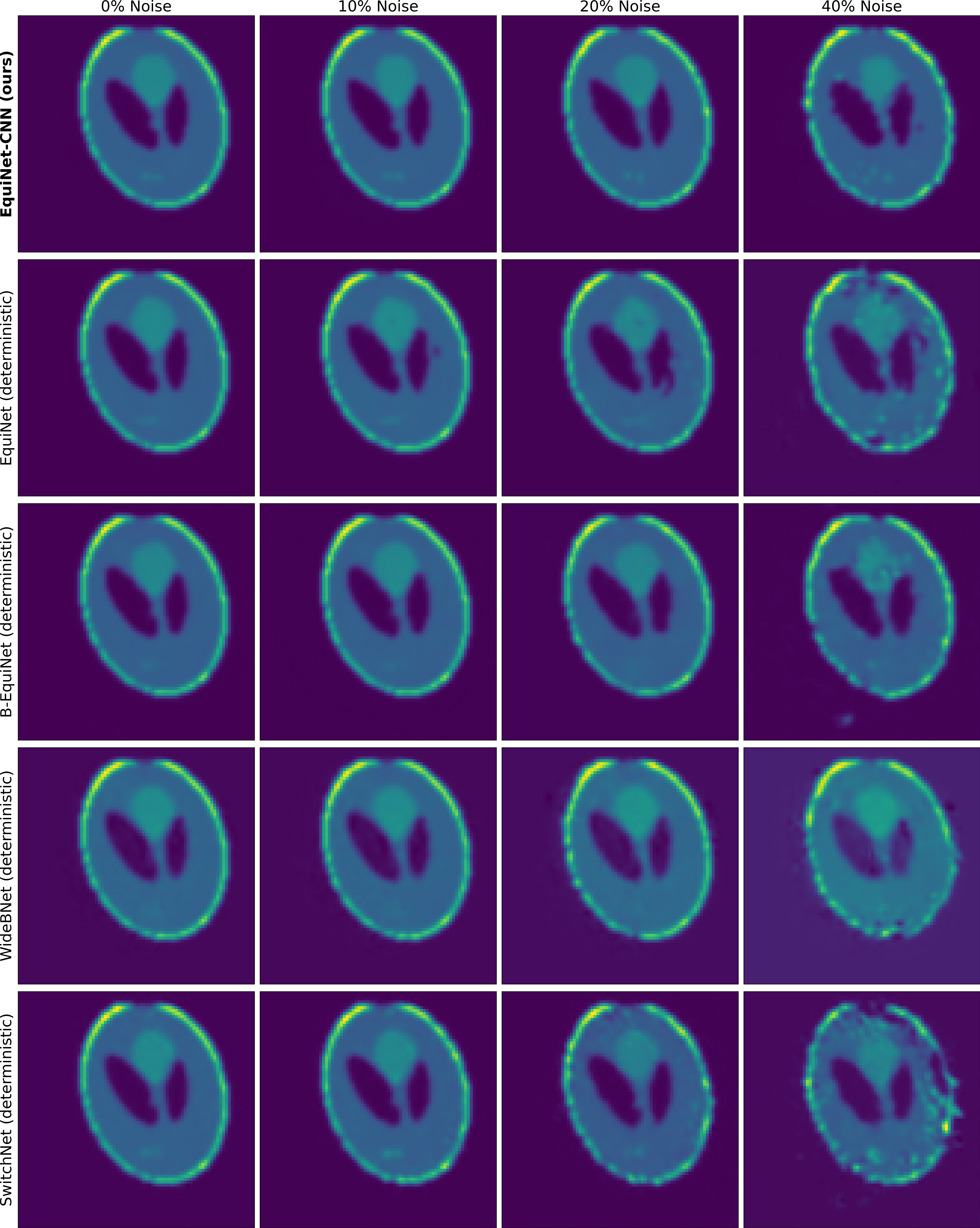
Figure 19: Comparison of reconstructions from EquiNet-CNN and baseline deterministic models on Shepp-Logan dataset as noise increases from 0% to 40%.

5.13 Mixed datasets and Generalization

We also consider how well our methodology behaves with more complex distributions and also with out-of-distribution samples.

To assess the behavior of our networks with more complex distributions, we train our network, along with some of the baselines, using a mix of all synthetic datasets: Shepp-Logan, 3-5-10h Triangles, and 10h Overlapping Squares. We then compute the RRMSE, MELR, and SD of the respective reconstructions for each dataset separately, which are shown in Table 13. From Table 13, we can observe that EquiNet-CNN is able to generate samples for each dataset with relatively high accuracy when training with the mixed dataset, in contrast with other deterministic models. This observation indicates that EquiNet-CNN has, in general, higher capacity than the alternatives, and it is capable of learning more distributions of scatterers with higher intrinsic dimensionality when compared to other ML-based methods

Model	RRMSE	MELR	SD
		$(\times 10^{-2})$
Shepp-Logan (Reference SD: 14.406)
EquiNet-CNN	1.583%	1.899	3.774
EquiNet (deterministic)	4.360%	16.033	4.155
B-EquiNet (deterministic)	3.581%	8.748	4.047
WideBNet (deterministic)	6.971%	28.073	4.512
SwitchNet (deterministic)	6.279%	21.042	4.407
3-5-10h Triangles (Reference SD: 2.833)
EquiNet-CNN	6.161%	3.533	1.044
EquiNet (deterministic)	19.055%	30.432	1.297
B-EquiNet (deterministic)	12.404%	13.696	1.177
WideBNet (deterministic)	36.077%	117.196	1.591
SwitchNet (deterministic)	32.460%	93.747	1.520
10h Overlapping Squares (Reference SD: 11.183)
EquiNet-CNN	2.579%	2.857	3.962
EquiNet (deterministic)	12.692%	35.055	5.078
B-EquiNet (deterministic)	10.687%	26.418	4.860
WideBNet (deterministic)	19.039%	104.101	5.765
SwitchNet (deterministic)	15.277%	42.314	5.365

Table 13: Comparison of RRMSE, MELR, and SD of reconstructions for each dataset (Shepp-Logan, 3-5-10h Triangles, and 10h Overlapping Squares) between EquiNet-CNN and deterministic models (EquiNet, B-EquiNet, WideBNet, and SwitchNet). All of the models are trained with the mixed dataset. The best performance metrics for each dataset are indicated in bold.

We also consider performance of EquiNet-CNN on datasets that are out-of-distribution, in contrast to the within-distribution training dataset. For such assesment, we trained EquiNet-CNN on the 10h Overlapping Squares dataset and we tested the model on the out-of-distrbution Shepp-Logan and 3-5-10h Triangles dataset. Figure 20 shows reconstructions of the model from both within-distribution 3-5-10h Triangles dataset and out-of-distribution Shepp-Logan and 10h Overlapping Squares datasets. Although, our model, given its statistical nature, generalizes poorly, it is still able to locate and provide some features of the Shepp-Logan phantom.

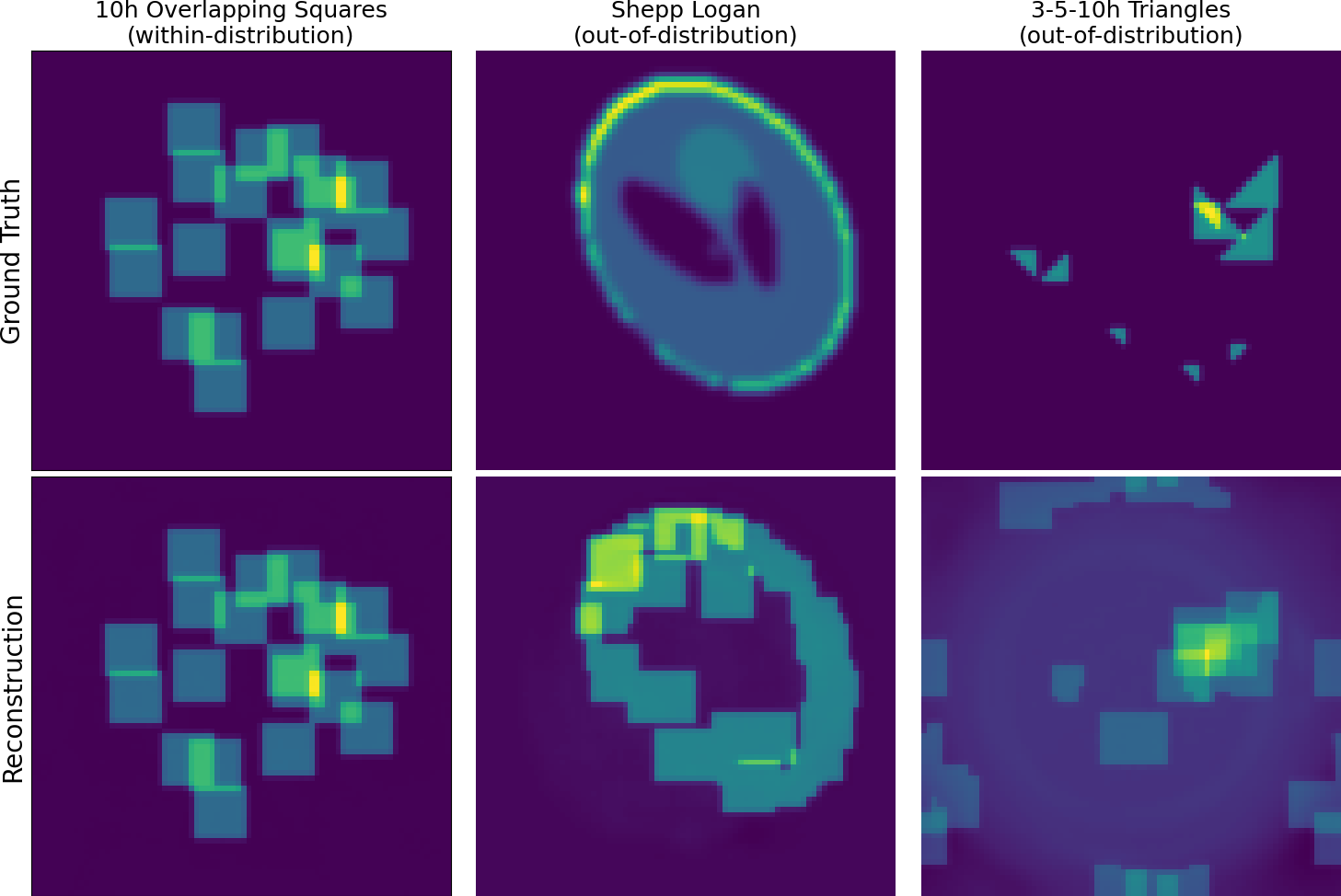
Figure 20: Reconstructions of out-of-distribution Shepp-Logan and 3-5-10h Triangles datasets from EquiNet-CNN trained on within-distribution 10h Overlapping Squares dataset.

6 Conclusion

By factorizing the score function according to the filtered back-projection formula into back-projection steps that compute a latent representation and a conditional scoring function conditioned on this latent representation, we provide a powerful yet straightforward framework that combines generative AI methods with analytical knowledge of the underlying physical problem. By designing networks that carefully exploit this knowledge, we produce state-of-the-art reconstructions with built-in uncertainty that outperform existing methods, even in the notoriously difficult multiple scattering cases.

Unfortunately, as shown in Section 5.13, our methodology still relies on distributions of scatterers with relatively low-intrinsic dimension. Although it outperforms other methods when introducing more complex distributions, it still generalizes poorly, meaning that it fails to fully capture the underlying physics of wave propagation. Future research directions include how to reincorporate the physics back into the sampling process by leveraging the PDE, and how to automatically check if an input is out-of-distribution, thus re-weighting the prior during the sampling process.

7 Acknowledgement

The work of Q.~L. is supported by the National Science Foundation under the grant DMS-2308440. The work of M.~G. is partially supported by the National Science Foundation under the grant DMS-2012292. The views expressed in the article do not necessarily represent the views of the any funding agencies. The authors are grateful for the support.

Appendix A Proof of the Proposition 2.1

We should note that the injectivity of $F^{\ast}$ plays an important role that allows us to transit from using $\Lambda$ as the condition to using $\alpha_{\Lambda}$.

Indeed, since $F^{\ast}$ is injective, it is invertible within the range of $F^{\ast}$, making $\Lambda=(F^{\ast})^{-1}\alpha_{\Lambda}$. In this appendix section, we prove this injectivity.

Lemma A.1 (Jacobi–Anger Expansion [119]).

For $z,\theta\in\mathbb{R}$, the following identity holds:

$$e^{iz\cos\theta}=\sum_{n=-\infty}^{\infty}i^{n}J_{n}(z)e^{in\theta}\,,$$ (79)

where $J_{n}(z)$ denotes the $n$-th Bessel function of the first kind.

Lemma A.2.

For any $k,n\in\mathbb{N}$ and $a\in\mathbb{R}^{+}$, the following integrals hold:

$$\int_{0}^{\infty}J_{n}(x)J_{n-k}(x)J_{k}(ax)x\,dx=\frac{\cos(n(\pi-2\phi_{a})-k(\pi-\phi_{a}))}{\pi a\sin(\phi_{a})}\,,$$ (80)

$$\int_{0}^{\infty}J_{n}(x)J_{n-k}(x)Y_{k}(ax)x\,dx=\frac{\sin(n(\pi-2\phi_{a})-k(\pi-\phi_{a}))}{\pi a\sin(\phi_{a})}\,,$$ (81)

where $J_{n}(z)$ is the $n$-th Bessel function of the first kind, $Y_{n}(z)$ is the $n$-th Bessel function of the second kind, and $\phi_{a}$ is the base angle of the isosceles triangle with side lengths 1, 1, and $a$.

Proof.

See Sections B and C in [120] for proofs of the first and second formulas, respectively. ∎

Proposition A.3 (A rewriting of Proposition 2.1).

The back-scattering operator $(F^{\omega})^{\ast}:L^{2}([0,2\pi]^{2})\rightarrow L^{2}(\mathbb{R}^{2})$ is injective.

Proof.

We represent the intermediate field in the polar coordinates, given by (56), we have

$$\alpha^{\omega}(\theta,\rho)=((F^{\omega})^{*}\Lambda^{\omega})(\theta,\rho)=\iint_{[0,2\pi]^{2}}e^{i\omega\rho\cos(r)}e^{-i\omega\rho\cos(s)}\Lambda^{\omega}(r+\theta,s+\theta)\,dr\,ds\,.$$ (82)

To prove $(F^{\omega})^{\ast}$ is injective, we set $(F^{\omega})^{*}\Lambda^{\omega}=0$ and we aim to show $\Lambda^{\omega}=0$ in $L^{2}([0,2\pi]^{2})$.

First, we represent $\Lambda^{\omega}$ by a complex Fourier series

$$\Lambda^{\omega}(r,s)=\sum_{p,q=-\infty}^{\infty}c_{p,q}e^{ipr}e^{iqs}\,.$$ (83)

Thus, applying the phase shift

$$\Lambda^{\omega}(r+\theta,s+\theta)=\sum_{p,q=-\infty}^{\infty}c_{p,q}e^{i(p+q)\theta}e^{ipr}e^{iqs}\,.$$ (84)

Then, using the Jacobi-Anger Expansion A.1 and the fact that $J_{n}(-x)=(-1)^{n}J_{n}(x)$, we have

$$e^{i\omega\rho\cos(r)}=\sum_{n=-\infty}^{\infty}i^{n}J_{n}(\omega\rho)e^{inr}\,,$$ (85)

and

$$e^{-i\omega\rho\cos(s)}=e^{-i\omega\rho\cos(-s)}=\sum_{m=-\infty}^{\infty}(-i)^{m}J_{m}(\omega\rho)e^{-ims}\,.$$ (86)

Substituting the expansions and the shifted $\Lambda^{\omega}$ into the integral, we have

$$\iint_{[0,2\pi]^{2}}\left(\sum_{n=-\infty}^{\infty}i^{n}J_{n}(\omega\rho)e^{inr}\right)\left(\sum_{m=-\infty}^{\infty}(-i)^{m}J_{m}(\omega\rho)e^{-ims}\right)\left(\sum_{p,q=-\infty}^{\infty}c_{p,q}e^{i(p+q)\theta}e^{ipr}e^{iqs}\right)\,ds\,dr\,,$$ (87)

$$=\sum_{n,m,p,q=-\infty}^{\infty}i^{n}(-i)^{m}J_{n}(\omega\rho)J_{m}(\omega\rho)c_{p,q}e^{i(p+q)\theta}\iint_{[0,2\pi]^{2}}e^{i(n+p)r}e^{i(-m+q)s}\,dr\,ds\,,$$

where the equality follows from the Fubini’s theorem.

The exponential functions $e^{inr}$ and $e^{ims}$ are orthogonal over $[0,2\pi]$

$$\int_{0}^{2\pi}e^{i(n+p)r}\,dr=2\pi\delta_{n+p,0}\,,\quad\int_{0}^{2\pi}e^{i(-m+q)s}\,ds=2\pi\delta_{-m+q,0}\,.$$ (88)

Substituting back and simplifying, for almost every $\theta\in[0,2\pi]$ and $\rho\in[0,\infty)$, we have

$$\sum_{n,m=-\infty}^{\infty}i^{n-m}J_{n}(\omega\rho)J_{m}(\omega\rho)c_{-n,m}e^{-i(n-m)\theta}=0\,.$$ (89)

By using Fubini’s theorem and setting $k=n-m$, our expression becomes

$$\sum_{k=-\infty}^{\infty}i^{k}\left(\sum_{n=-\infty}^{\infty}J_{n}(\omega\rho)J_{n-k}(\omega\rho)c_{-n,n-k}\right)e^{-ik\theta}=0\,.$$ (90)

For almost every $\rho\in[0,\infty)$, the series on the left can be viewed as a Fourier series in $\theta$ of a zero function. Consequently, all Fourier coefficients must be zero

$$\sum_{n=-\infty}^{\infty}J_{n}(\omega\rho)J_{n-k}(\omega\rho)c_{-n,n-k}=0\quad\forall k\in\mathbb{Z}\,.$$ (91)

Now fix a $k\in\mathbb{Z}$, for all $a\in\mathbb{R}^{+}$, we multiply the series on the left by $J_{k}(a\omega\rho)\omega^{2}\rho$ and integrate over $\rho$ from $0$ to $\infty$. By the Fubini’s theorem and the Lemma A.2, we have

$$\int_{0}^{\infty}\left(\sum_{n=-\infty}^{\infty}J_{n}(\omega\rho)J_{n-k}(\omega\rho)c_{-n,n-k}\right)J_{k}(a\omega\rho)\omega^{2}\rho\,d\rho\,,$$

$$= \sum_{n=-\infty}^{\infty}c_{-n,n-k}\int_{0}^{\infty}J_{n}(\omega\rho)J_{n-k}(\omega\rho)J_{k}(a\omega\rho)\omega\rho\,d(\omega\rho)\,,$$

$$= \sum_{n=-\infty}^{\infty}c_{-n,n-k}\frac{\cos(n(\pi-2\phi_{a})-k(\pi-\phi_{a}))}{\pi a\sin(\phi_{a})}\,,$$

where $\phi_{a}\in(0,\pi)$ for $a\in\mathbb{R}^{+}$. Hence, our expression becomes

$$\sum_{n=-\infty}^{\infty}c_{-n,n-k}\cos(n(\pi-2\phi_{a})-k(\pi-\phi_{a}))=0\,.$$ (92)

By the Lemma A.2, and a similar computation with the series multiplied by $Y_{k}(a\omega\rho)\omega^{2}\rho$, we have

$$\sum_{n=-\infty}^{\infty}c_{-n,n-k}\sin(n(\pi-2\phi_{a})-k(\pi-\phi_{a}))=0\,.$$ (93)

Therefore, by combining the two and simplifying, for all $a\in\mathbb{R}^{+}\implies\pi-2\phi_{a}\in(-\pi,\pi)$, we have

$$\sum_{n=-\infty}^{\infty}c_{-n,n-k}e^{in(\pi-2\phi_{a})}=0\,.$$ (94)

We can view the sum as a Fourier series in $\phi_{a}\in(0,\pi)$ of a zero function. Hence, coefficients $c_{-n,n-k}$ for $k,n\in\mathbb{N}$ must be $0$. Since $k$ is arbitrary, all Fourier coefficients $c_{k,l}$ in the original representation of $\Lambda^{\omega}$ are $0$. By the Parseval’s theorem, we have $\Lambda^{\omega}=0$. Therefore, we can conclude that $(F^{\omega})^{\ast}$ is injective.

∎

Appendix B Proof of the Theorem 4.4

Throughout this section, we define the inner product on $\mathbb{R}^{n_{\eta}\times n_{\eta}}$ by the usual dot product

$$\langle v,w\rangle=v\cdot w\,.$$ (95)

Lemma B.1.

The inverse of the translation operator $T_{\bm{a}}$ is $T_{-\bm{a}}$:

$$(T_{\bm{a}})^{-1}=T_{-\bm{a}}\,.$$ (96)

Proof.

For all $v\in\mathbb{R}^{n_{\eta}\times n_{\eta}}$, $\bm{a}\in\mathbb{N}_{\eta}^{2}$ and $\bm{y}\in\mathbb{N}_{\eta}^{2}$, we have

$$((T_{\bm{a}}\circ T_{-\bm{a}})v)_{\bm{y}}=v_{\bm{y}+\bm{a}-\bm{a}}=v_{\bm{y}}\,.$$ (97)

Therefore, we have

$$T_{\bm{a}}\circ T_{-\bm{a}}=\bm{I}\,,$$ (98)

where $\bm{I}$ is the identity operator on $\mathbb{R}^{n_{\eta}\times n_{\eta}}$. ∎

Lemma B.2.

The translation operator $T_{\bm{a}}$ is a unitary linear transformation. Consequently, the Jacobian $J_{T_{\bm{a}}}$ of the change of variables under the transformation $T_{\bm{a}}$ satisfies

$$|\det J_{T_{\bm{a}}}|=1\,,$$ (99)

and by Lemma B.1, we have

$$\langle T_{\bm{a}}v,w\rangle=\langle v,T_{-\bm{a}}w\rangle\,.$$ (100)

Proof.

for any $v,w\in\mathbb{R}^{n_{\eta}\times n_{\eta}}$, and any $\bm{a}\in\mathbb{N}_{\eta}^{2}$, as $T_{\bm{a}}$ is invertible, it suffices to show

$$\langle T_{\bm{a}}v,T_{\bm{a}}w\rangle=\sum_{\bm{y}\in\mathbb{N}_{\eta}^{2}}v_{\bm{y}-\bm{a}}w_{\bm{y}-\bm{a}}=\sum_{\bm{y}\in\mathbb{N}_{\eta}^{2}}v_{\bm{y}}w_{\bm{y}}=\langle v,w\rangle\,.$$ (101)

∎

Lemma B.3.

Let $\mathsf{F}^{\omega}$ be the discretized forward map, and $(\mathsf{F}^{\omega})^{*}$ be the discretized back-scattering operator, see Section 2.3. Then, for any $\bm{a}\in\mathbb{N}_{\eta}^{2}$, $(\mathsf{F}^{\omega})^{*}\mathsf{F}^{\omega}$ commutes with the translation operator $T_{\bm{a}}$, i.e.

$$((\mathsf{F}^{\omega})^{*}\mathsf{F}^{\omega})\circ T_{\bm{a}}=T_{\bm{a}}\circ((\mathsf{F}^{\omega})^{*}\mathsf{F}^{\omega})\,.$$ (102)

Proof.

For the discretization of $\eta$, see Section 2.3, we used a Cartesian mesh of $n_{\eta}\times n_{\eta}$ grids for the physical domain $\Omega=[-0.5,0.5]^{2}$. We further denote the grid points by $\bm{x}_{(i,j)}$, so that

$$\bm{\eta}_{(i,j)}=\eta(\bm{x}_{(i,j)})\,.$$ (103)

Similarly, we denote the grid points from the discretization of $\mathbb{S}^{1}$ by $\bm{s}_{(n)}$ and $\bm{r}_{(m)}$, where

$$\bm{s}_{(n)}=(\cos(s_{n}),\sin(s_{n}))\text{\quad and\quad}\bm{r}_{(m)}=(\cos(r_{m}),\sin(r_{m}))\,.$$ (104)

For any $\bm{x}\in\mathbb{R}^{2}$, we define $\bm{x}\mod\Omega$ as the operation that maps $\bm{x}$ to the physical domain $\Omega$ by

$$\bm{x}\mod\Omega=((\bm{x}+\bm{0.5})\mod\bm{1})-\bm{0.5}\,,$$ (105)

where $\bm{c}=(c,c)\in\mathbb{R}^{2}$, and the modulo operation is applied element-wise.

Then, we have the following identity

$$(T_{\bm{a}}\bm{\eta})(\bm{x})=\eta(\bm{x}-\bm{a}/n_{\eta}\mod\Omega)\,.$$ (106)

It is straightforward to find

$$((\mathsf{F}^{\omega})^{*}\mathsf{F}^{\omega}\bm{\eta})(\bm{y}) =\sum_{n,m=1}^{n_{\mathrm{sc}}}e^{i\omega(\bm{r}_{(m)}-\bm{s}_{(n)})\cdot\bm{y}}\sum_{i,j=1}^{n_{\eta}}e^{-i\omega(\bm{r}_{(m)}-\bm{s}_{(n)})\cdot\bm{x}_{(i,j)}}\eta(\bm{x}_{(i,j)})\,,$$ (107)

$$=\sum_{n,m=1}^{n_{\mathrm{sc}}}\sum_{i,j=1}^{n_{\eta}}e^{i\omega(\bm{r}_{(m)}-\bm{s}_{(n)})\cdot(\bm{y}-\bm{x}_{(i,j)})}\eta(\bm{x}_{(i,j)})\,.$$

By applying a translation operator and use the identity in (106), similar to (107), we have

$$((\mathsf{F}^{\omega})^{*}\mathsf{F}^{\omega}T_{\bm{a}}\bm{\eta})(\bm{y}) =\sum_{n,m=1}^{n_{\mathrm{sc}}}\sum_{i,j=1}^{n_{\eta}}e^{i\omega(\bm{r}_{(m)}-\bm{s}_{(n)})\cdot(\bm{y}-\bm{x}_{(i,j)})}\eta(\bm{x}_{(i,j)}-\bm{a}/n_{\eta}\mod\Omega)\,,$$ (108)

$$=\sum_{n,m=1}^{n_{\mathrm{sc}}}\sum_{i,j=1}^{n_{\eta}}e^{i\omega(\bm{r}_{(m)}-\bm{s}_{(n)})\cdot(\bm{y}-(\bm{x}_{(i,j)}+\bm{a}/n_{\eta}\mod\Omega))}\eta(\bm{x}_{(i,j)})\,,$$

$$=\sum_{n,m=1}^{n_{\mathrm{sc}}}\sum_{i,j=1}^{n_{\eta}}e^{i\omega(\bm{r}_{(m)}-\bm{s}_{(n)})\cdot((\bm{y}-\bm{a}/n_{\eta}\mod\Omega)-\bm{x}_{(i,j)})}\eta(\bm{x}_{(i,j)})\,,$$

$$=(T_{\bm{a}}(\mathsf{F}^{\omega})^{*}\mathsf{F}^{\omega}\bm{\eta})(\bm{y})\,.$$

Since $\eta$ is arbitrary, we can conclude that

$$(\mathsf{F}^{\omega})^{*}\mathsf{F}^{\omega}\circ T_{\bm{a}}=T_{\bm{a}}\circ(\mathsf{F}^{\omega})^{*}\mathsf{F}^{\omega}\,.$$ (109)

∎

Lemma B.4.

Suppose that an operator $\mathcal{P}\in C^{1}(\mathbb{R}^{n_{\eta}\times n_{\eta}})^{\otimes 2}$ acting on $(v,w)\in(\mathbb{R}^{n_{\eta}\times n_{\eta}})^{\otimes 2}$ satisfies translational invariance

$$\mathcal{P}(T_{\bm{a}}v,T_{\bm{a}}w)=\mathcal{P}(v,w)\quad\forall\bm{a}\in\mathbb{N}_{\eta}^{2}\,,$$ (110)

then the gradient of $\mathcal{P}$ with respect to $v$, denoted as $\nabla_{v}\mathcal{P}$, is translationally equivariant.

Proof.

For any $\bm{a}\in\mathbb{N}_{\eta}^{2}$, by the definition of the gradient, for a small perturbation $\epsilon h$ such that $\epsilon>0$ and $h\in\mathbb{R}^{n_{\eta}\times n_{\eta}}$:

$$\mathcal{P}(T_{\bm{a}}v+\epsilon h,T_{\bm{a}}w)=\mathcal{P}(T_{\bm{a}}v,T_{\bm{a}}w)+\epsilon\langle\nabla_{v}\mathcal{P}(T_{\bm{a}}v,T_{\bm{a}}w),h\rangle+o(\epsilon)\,.$$ (111)

By the assumption in this lemma, the fact that the inverse operator of $T_{\bm{a}}$ is $T_{-\bm{a}}$ as shown in Lemma B.1, and $T_{\bm{a}}$ is unitary as shown in Lemma B.2, we have

$$\mathcal{P}(T_{\bm{a}}v+\epsilon h,T_{\bm{a}}w) =\mathcal{P}(v+\epsilon T_{-\bm{a}}h,w)\,,$$ (112)

$$=\mathcal{P}(v,w)+\epsilon\langle\nabla_{v}\mathcal{P}(v,w),T_{-\bm{a}}h\rangle+o(\epsilon)\,,$$

$$=\mathcal{P}(T_{\bm{a}}v,T_{\bm{a}}w)+\epsilon\langle T_{\bm{a}}\nabla_{v}\mathcal{P}(v,w),h\rangle+o(\epsilon)\,.$$

Comparing (111) and (112), noting that $h\in\mathbb{R}^{n_{\eta}\times n_{\eta}}$ is arbitrary, we have:

$$\nabla_{v}\mathcal{P}(T_{\bm{a}}v,T_{\bm{a}}w)=T_{\bm{a}}\nabla_{v}\mathcal{P}(v,w)\quad\forall a\in\mathbb{N}_{\eta}^{2}\,,$$ (113)

concluding the lemma. ∎

Lemma B.5.

With the same assumptions as in Theorem 4.4, denote $\bm{\eta}_{0}$ the ground truth perturbation that corresponds to the intermediate field $\bm{\alpha}$, we have

1. The operator $\mathcal{U}:(\mathbb{R}^{n_{\eta}\times n_{\eta}})^{\otimes 2}\rightarrow\mathbb{R}$ defined as $\mathcal{U}(\bm{\eta},\bm{\eta}_{0})=p_{t}(\bm{\eta}|\bm{\eta}_{0})$ is translationally invariant.

2. The operator $\mathcal{W}:(\mathbb{R}^{n_{\eta}\times n_{\eta}})^{\otimes 2}\rightarrow\mathbb{R}$ defined as $\mathcal{W}(\bm{\alpha},\bm{\eta}_{0})=p_{0}(\bm{\eta}_{0}|\bm{\alpha})$ is translationally invariant.

Proof.

1. As discussed in Section 3, $p_{t}(\bm{\eta}|\bm{\eta}_{0})$ is the perturbation kernel (see (36)):

   $$p_{t}(\bm{\eta}|\bm{\eta}_{0})=\mathcal{N}(\bm{\eta};s(t)\bm{\eta}_{0},s^{2}(t)\sigma^{2}(t)\bm{I})=\exp\left(-\frac{\|\bm{\eta}-s(t)\bm{\eta}_{0}\|^{2}}{2s^{2}(t)\sigma^{2}(t)}\right)\cdot\frac{1}{Z}\,,$$ (114)

   where $Z$ is the normalization constant.

   Since the translation operator is unitary, $\forall\bm{a}\in\mathbb{N}_{\eta}^{2}$, we have

   $$p_{t}(T_{\bm{a}}\bm{\eta}|T_{\bm{a}}\bm{\eta}_{0}) =\exp\left(-\frac{\|T_{\bm{a}}(\bm{\eta}-s(t)\bm{\eta}_{0})\|^{2}}{2s^{2}(t)\sigma^{2}(t)}\right)\cdot\frac{1}{Z}\,,$$

   $$=\exp\left(-\frac{\|\bm{\eta}-s(t)\bm{\eta}_{0}\|^{2}}{2s^{2}(t)\sigma^{2}(t)}\right)\cdot\frac{1}{Z}\,,$$

   $$=p_{t}(\bm{\eta}|\bm{\eta}_{0}).$$

2. Notice that the marginal distributions $p_{0}(\bm{\eta})=p_{\text{data}}(\bm{\eta})$. By the assumption that $\mathcal{P}(\bm{\alpha},\bm{\eta}_{0})=p_{0}(\bm{\alpha}|\bm{\eta}_{0})$ and $p_{\text{data}}(\bm{\eta})$ are translationally invariant, for all $\bm{a}\in\mathbb{N}_{\eta}^{2}$, we have

   $$p_{0}(T_{\bm{a}}\bm{\alpha},T_{\bm{a}}\bm{\eta}_{0})=p_{0}(T_{\bm{a}}\bm{\alpha}|T_{\bm{a}}\bm{\eta}_{0})p_{\text{data}}(T_{\bm{a}}\bm{\eta}_{0})=p_{0}(\bm{\alpha}|\bm{\eta}_{0})p_{\text{data}}(\bm{\eta}_{0})=p_{0}(\bm{\alpha},\bm{\eta}_{0})\,.$$ (115)

   Now it suffices to show the marginal distributions

   $$p_{0}(T_{\bm{a}}\bm{\alpha})=p_{0}(\bm{\alpha})\quad\forall\bm{a}\in\mathbb{N}_{\eta}^{2}\,.$$ (116)

   According to the definition, this amounts to show

   $$\int_{\bm{\eta}_{0}\in\mathbb{R}^{n_{\eta}\times n_{\eta}}}p_{0}(T_{\bm{a}}\bm{\alpha},\bm{\eta}_{0})\,d\bm{\eta}_{0}=\int_{\bm{\eta}_{0}\in\mathbb{R}^{n_{\eta}\times n_{\eta}}}p_{0}(\bm{\alpha},\bm{\eta}_{0})\,d\bm{\eta}_{0}\quad\forall\bm{a}\in\mathbb{N}_{\eta}^{2}\,.$$ (117)

   This is true because:

   $$p_{0}(T_{\bm{a}}\bm{\alpha}) =\int_{\bm{\eta}_{0}\in\mathbb{R}^{n_{\eta}\times n_{\eta}}}p_{0}(T_{\bm{a}}\bm{\alpha},\bm{\eta}_{0})\,d\bm{\eta}_{0}\,,$$ (118)

   $$=\int_{\bm{\zeta}_{0}\in\mathbb{R}^{n_{\eta}\times n_{\eta}}}p_{0}(T_{\bm{a}}\bm{\alpha},T_{\bm{a}}\bm{\zeta}_{0})|\det J_{T_{\bm{a}}}|\,d\bm{\zeta}_{0}\,,$$

   $$=\int_{\bm{\zeta}_{0}\in\mathbb{R}^{n_{\eta}\times n_{\eta}}}p_{0}(\bm{\alpha},\bm{\zeta}_{0})\,d\bm{\zeta}_{0}\,,$$

   $$=p_{0}(\bm{\alpha})\quad\forall\bm{a}\in\mathbb{N}_{\eta}^{2}\,.$$

   where we used change of variable $\bm{\eta}_{0}=T_{\bm{a}}\bm{\zeta}_{0}$ in the second equation, and applied Lemma B.2 in the third. Then using the definition of the conditional distribution,

   $$p_{0}(T_{\bm{a}}\bm{\eta}_{0}|T_{\bm{a}}\bm{\alpha})=\frac{p_{0}(T_{\bm{a}}\bm{\alpha},T_{\bm{a}}\bm{\eta}_{0})}{p_{0}(T_{\bm{a}}\bm{\alpha})}=\frac{p_{0}(\bm{\alpha},\bm{\eta}_{0})}{p_{0}(\bm{\alpha})}=p_{0}(\bm{\eta}_{0}|\bm{\alpha})\quad\forall\bm{a}\in\mathbb{N}_{\eta}^{2}\,,$$ (119)

   concluding the proof.

∎

Theorem B.6 (A rewriting of Theorem 4.4).

With $\bm{\alpha}$, $\bm{\eta}$ and $p_{t}$ defined above, if $\mathcal{P}(\bm{\alpha},\bm{\eta})=p_{0}(\bm{\alpha}|\bm{\eta})$ and $p_{\text{data}}(\bm{\eta})$ are both translationally invariant, then the physics-aware score function $\nabla_{\bm{\eta}}\log p_{t}(\bm{\eta}|\bm{\alpha})$ is translationally equivariant. More specifically, assume: $p_{0}(T_{\bm{a}}\bm{\alpha}|T_{\bm{a}}\bm{\eta})=p_{0}(\bm{\alpha}|\bm{\eta})$ and $p_{\text{data}}(T_{\bm{a}}\bm{\eta})=p_{\text{data}}(\bm{\eta})$ for all $\bm{a}\in\mathbb{N}_{\eta}^{2}$, then for $p_{t}\in C^{1}(\mathbb{R}^{n_{\eta}\times n_{\eta}})^{\otimes 2}$ and $p_{t}>0$:

$$\nabla_{\bm{\eta}}\log p_{t}(T_{\bm{a}}\bm{\eta}|T_{\bm{a}}\bm{\alpha})=T_{\bm{a}}\nabla_{\bm{\eta}}\log p_{t}(\bm{\eta}|\bm{\alpha})\quad\forall\bm{a}\in\mathbb{N}_{\eta}^{2}\,,$$ (120)

i.e. $\mathcal{Q}(\bm{\eta},\bm{\alpha})=\nabla_{\bm{\eta}}\log p_{t}(\bm{\eta}|\bm{\alpha})$ is translational equivariant.

Proof.

From the forward SDE (33), it can be seen that conditioned on $\bm{\eta}_{0}$, $\bm{\eta}_{t}$ and $\bm{\alpha}$ are independent, so

$$p_{t}(\bm{\eta},\bm{\alpha}|\bm{\eta}_{0})=p_{t}(\bm{\eta}|\bm{\eta}_{0})p_{0}(\bm{\alpha}|\bm{\eta}_{0})\implies p_{t}(\bm{\eta}|\bm{\alpha},\bm{\eta}_{0})=p_{t}(\bm{\eta}|\bm{\eta}_{0})\,.$$ (121)

As a consequence

$$p_{t}(\bm{\eta}|\bm{\alpha}) =\int_{\bm{\eta}_{0}\in\mathbb{R}^{n_{\eta}\times n_{\eta}}}p_{t}(\bm{\eta},\bm{\eta}_{0}|\bm{\alpha})\,d\bm{\eta}_{0}\,,$$ (122)

$$=\int_{\bm{\eta}_{0}\in\mathbb{R}^{n_{\eta}\times n_{\eta}}}p_{t}(\bm{\eta}|\bm{\eta}_{0},\bm{\alpha})p_{0}(\bm{\eta}_{0}|\bm{\alpha})\,d\bm{\eta}_{0}\,,$$

$$=\int_{\bm{\eta}_{0}\in\mathbb{R}^{n_{\eta}\times n_{\eta}}}p_{t}(\bm{\eta}|\bm{\eta}_{0})p_{0}(\bm{\eta}_{0}|\bm{\alpha})\,d\bm{\eta}_{0}\,.$$

where we used (121) in the third equation. Similarly,

$$p_{t}(T_{\bm{a}}\bm{\eta}|T_{\bm{a}}\bm{\alpha}) =\int_{\bm{\eta}_{0}\in\mathbb{R}^{n_{\eta}\times n_{\eta}}}p_{t}(T_{\bm{a}}\bm{\eta}|\bm{\eta}_{0})p_{0}(\bm{\eta}_{0}|T_{\bm{a}}\bm{\alpha})\,d\bm{\eta}_{0}\,,$$ (123)

$$=\int_{\bm{\zeta}_{0}\in\mathbb{R}^{n_{\eta}\times n_{\eta}}}p_{t}(T_{\bm{a}}\bm{\eta}|T_{\bm{a}}\bm{\zeta}_{0})p_{0}(T_{\bm{a}}\bm{\zeta}_{0}|T_{\bm{a}}\bm{\alpha})|\det J_{T_{\bm{a}}}|\,d\bm{\zeta}_{0}\,,$$

$$=\int_{\bm{\zeta}_{0}\in\mathbb{R}^{n_{\eta}\times n_{\eta}}}p_{t}(\bm{\eta}|\bm{\zeta}_{0})p_{0}(\bm{\zeta}_{0}|\bm{\alpha})\,d\bm{\zeta}_{0}\,,$$

$$=p_{t}(\bm{\eta}|\bm{\alpha})\,,$$

where we used a change of variable $\bm{\eta}_{0}=T_{\bm{a}}\bm{\zeta}_{0}$ in the second equation, and called Lemma B.2, and Lemma B.5 in the third equation. Consequently, the operator $\mathcal{R}(\bm{\eta},\bm{\alpha})=\log p_{t}(\bm{\eta}|\bm{\alpha})$ satisfies translational invariance. By Lemma B.4, we can conclude that $\nabla_{\bm{\eta}}\mathcal{R}(\bm{\eta},\bm{\alpha})=\nabla_{\bm{\eta}}\log p_{t}(\bm{\eta}|\bm{\alpha})$ satisfies translational equivariance. ∎

Appendix C Metrics

Relative Root Mean Square Error (RRMSE)

This is a very well-known metric to primarily quantify the quality of our samples. We define it as follows,

$$\text{RRMSE}=\frac{1}{N_{t}}\sum_{i=1}^{N_{t}}\frac{\|\bm{\eta}_{i}-\bm{\eta}_{0}\|}{\|\bm{\eta}_{0}\|}$$ (124)

where $N_{t}$ is the size of the testing set, $\bm{\eta_{i}}$ is the sample generated for test $i$, $\bm{\eta}_{0}$ is the ground truth and the norm used is the Frobenius norm. In the case of the probabilistic norms we also take the average across all samples.

Continuous Ranked Probability Score (CRPS)

A good way to measure the efficacy of a probabilistic model is to compare the estimated probability distribution of $p$ to the ground truth value $\bm{\eta}_{0}$. For this task we use the CRPS [121] which is defined as follows,

$$\text{CRPS}(P,\bm{\eta}_{0})=\int(P(\bm{\eta})-\bm{1}_{\{\bm{\eta}\geq\bm{\eta}_{0}\}})^{2}d\bm{\eta}$$ (125)

where $P(\bm{\eta})$ is the CDF of $p$. However, in practice we will use the following equivalent formulation of the CRPS [122],

$$\text{CRPS}(P,\bm{\eta}_{0})=\mathbb{E}[\|\bm{\eta}-\bm{\eta}_{0}\|]-\frac{1}{2}\mathbb{E}[\|\bm{\eta}-\bm{\eta}^{\prime}\|]$$ (126)

where $\bm{\eta}$ and $\bm{\eta}^{\prime}$ are i.i.d samples of $p$.

Sinkhorn Divergence (SD)

One of the most popular metrics used to measure distance between distributions are the Optimal Transport (OT) based metrics, such as the Sinkhorn divergence, which we describe below. The field of OT is concerned with transforming (or transporting) one distribution into another, i.e., finding a map between them, in an optimal manner with respect to a pre-defined cost. The cost of the minimal (or optimal) transformation, often called the cost of the OT map, can then be used to define distances between distributions that ‘lifts’ the underlying metric $\mathrm{d}$ defined on $\mathcal{U}$ to one over the space of probability measures defined on $\mathcal{P}(\mathcal{U})$ [123].

In this context, we define the Kantorovich formulation of the OT cost [124] as

$$\mathcal{W}(\mu,\nu)=\min_{\gamma\in\Gamma(\mu,\nu)}\int_{\mathcal{U}\times\mathcal{U}}c(\bm{u},\bm{v})d\gamma(\bm{u},\bm{v}),$$

where $c:\mathcal{U}\times\mathcal{U}\rightarrow\mathbb{R}^{+}$ is an arbitrary cost function for transporting a unit of mass from $\bm{u}$ to $\bm{v},$ and $\Gamma$ is the set of joint distributions defined on $\mathcal{U}\times\mathcal{U}$ with correct marginals, i.e.,

$$\Gamma(\mu,\nu)=\{\gamma\in\mathcal{P}(\mathcal{U}\times\mathcal{U})\mid P_{1\#}\gamma=\mu,P_{2\#}\gamma=\nu\},$$

with $P_{1}(\bm{u},\bm{v})=\bm{u}$ and $P_{2}(\bm{u},\bm{v})=\bm{v}$ being simple projection operators. When $c(\bm{u},\bm{v})=\,d(\bm{u},\bm{v})^{p}$ with $p\geq 1$, then $\mathcal{W}^{1/p}$ is known as a Wasserstein-$p$ distance.

Practically, finding OT maps is a computationally expensive procedure. We therefore use entropic regularized versions of OT costs, which are amenable to efficient implementation on computational accelerators, by means of the Sinkhorn algorithm [125, 126]:

$$\mathcal{W}_{\varepsilon}(\mu,\nu)=\min_{\gamma\in\Gamma(\mu,\nu)}\mathcal{W}+\mathrm{KL(\gamma||\mu\otimes\nu)},$$ (127)

where $\mathrm{KL}$ is the Kullback-Leibler divergence, and $\mu\otimes\nu$ is the product of the marginal distributions. This gives rise to the Sinkhorn Divergence (SD):

$$\text{SD}(\mu,\nu)=2\mathcal{W}_{\varepsilon}(\mu,\nu)-\mathcal{W}_{\varepsilon}(\mu,\mu)-\mathcal{W}_{\varepsilon}(\nu,\nu),$$

which alleviates the entropic bias present in (127), i.e. $\mathcal{W}_{\varepsilon}(\mu,\mu)\neq 0.$ Of note, the SD can be shown to interpolate between a pure OT cost $\mathcal{W}$ (as $\varepsilon\rightarrow 0$) and a MMD (as $\varepsilon\rightarrow\infty$) [127, 128, 129].

We use the Optimal Transport Tools library [130] with its default hyperparameters to perform this computation.

Mean Energy Log Ratio (MELR)

The energy spectrum is one of the main metrics to quantitatively assess the quality of the resulting snapshots [109]. In a nutshell, the energy spectrum measures the energy in each Fourier mode and thereby providing insights into the similarity between the generated and reference samples.

The energy spectrum is defined as

$$E(k)=\sum_{|\underline{k}|=k}|\hat{\eta}(\underline{k})|^{2}=\sum_{|\underline{k}|=k}\left|\sum_{i,j}\eta(x_{i,j})\exp(-j2\pi\underline{k}\cdot x_{i,j}/L)\right|^{2}$$ (128)

where $k$ is the magnitude of the wave-number (wave-vector in 2D) $\underline{k}$, and $x_{i,j}$ is the underlying (possibly 2D) spatial grid. To assess the overall consistency of the spectrum between the generated and reference samples using a single scalar measure, we consider the mean energy log ratio (MELR):

$$\text{MELR}=\sum_{k}w_{k}\left|\log\left(E_{\text{pred}}(k)/E_{\text{ref}}(k)\right)\right|,$$ (129)

where $w_{k}$ represents the weight assigned to each $k$. We further define $w_{k}^{\text{unweighted}}=1/\text{card}(k)$ and $w_{k}^{\text{weighted}}=E_{\text{ref}}(k)/\sum_{k}E_{\text{ref}}(k)$. The latter skews more towards high-energy/low-frequency modes.

Appendix D Pseudocode for Algorithms

In this section we provide all the pseudocode for the different architectures presented in the paper.

Algorithm 2 Fourier Embedding

1:procedure FourierEmbedding($\sigma$)

2:     Calculate log frequencies:

3:      $\text{logfreqs}\leftarrow\text{Linspace}(0,\log(\text{max}\_{\text{freq}}),\text{emb\_dim}//2)$

4:     Compute Fourier features:

5:      $\sigma_{\text{freq}}\leftarrow\pi\cdot\exp(\text{logfreqs})\cdot\sigma$

6:      $\sigma_{\text{emb}}\leftarrow\text{Concatenate}([\sin(\sigma_{\text{freq}}),\cos(\sigma_{\text{freq}})],\text{axis}=-1)$

7:     Apply projection:

8:      $\sigma_{\text{emb}}\leftarrow\text{Dense}(\text{features}=2\cdot\text{emb\_dim})(\sigma_{\text{emb}})$

9:      $\sigma_{\text{emb}}\leftarrow\text{Swish}(\sigma_{\text{emb}})$

10:      $\sigma_{\text{emb}}\leftarrow\text{Dense}(\text{features}=\text{emb\_dim})(\sigma_{\text{emb}})$

11:     return $\sigma_{\text{emb}}$

12:end procedure

Algorithm 3 FiLM

1:procedure FiLM($\bm{x},\sigma_{\text{emb}}$)

2:      $\text{Affine}\leftarrow\text{Dense}(\text{features}=2\cdot\bm{x}.\text{shape}[-1])$

3:      $\text{params}\leftarrow\text{Affine}(\text{Swish}(\sigma_{\text{emb}}))$

4:      $\text{params}\leftarrow\text{params}.\text{reshape}(\text{params}.\text{shape}[:1]+(1,1)+\text{params}.\text{shape}[1:])$

5:      $\text{scale},\text{bias}\leftarrow\text{Split}(\text{params},2,\text{axis}=-1)$

6:     return $\bm{x}\cdot(\text{scale}+1)+\text{bias}$

7:end procedure

Algorithm 4 SqueezeBlock

1:procedure SqueezeBlock(out_channels,squeeze_channels)($\bm{x},\sigma_{\text{emb}}$)

2:     $\bm{h}\leftarrow\bm{x}$

3:     Two-layer convolution block with noise embedding in between:

4:     $\bm{h}\leftarrow\text{GroupNorm}(\bm{h}.\text{shape}[-1]//4)(\bm{h})$

5:     $\bm{h}\leftarrow\text{Swish}(\bm{h})$

6:     $\bm{h}\leftarrow\text{Conv2D}(\text{features}=\text{squeeze\_channels},\text{kernel\_size}=(3,3))(\bm{h})$

7:     $\bm{h}\leftarrow\text{GroupNorm}(\bm{h}.\text{shape}[-1]//4)(\bm{h})$

8:     $\bm{h}\leftarrow\text{FiLM}(\bm{h},\sigma_{\text{emb}})$

9:     $\bm{h}\leftarrow\text{Swish}(\bm{h})$

10:     $\bm{h}\leftarrow\text{Conv2D}(\text{features}=\text{out\_channels},\text{kernel\_size}=(3,3))(\bm{h})$

11:     Combine residual with skip:

12:     $\bm{x}\leftarrow\text{Dense}(\text{features}=\bm{h}.\text{shape}[-1])(\bm{x})$

13:     return $(\bm{x}+\bm{h})/\sqrt{2}$

14:end procedure

Algorithm 5 CNN-based representation

1:procedure CNN(num_embed, num_feature, num_conv, squeeze_ratio)($\bm{\eta},\bm{\alpha},\sigma$)

2:     $\bm{\alpha}\leftarrow\text{LayerNorm}(\bm{\alpha})$

3:     Condition Embedding:

4:     for $i\leftarrow 1$ to num_embed do

5:         $\text{tmp}\leftarrow\text{Conv2D}(\text{features}=6,\text{kernel\_size}=(3,3))(\bm{\alpha})$

6:         $\text{tmp}\leftarrow\text{Swish}(\text{tmp})$

7:         $\text{tmp}\leftarrow\text{Conv2D}(\text{features}=6,\text{kernel\_size}=(3,3))(\text{tmp})$

8:         $\bm{\alpha}\leftarrow\text{concatenate}([\bm{\alpha},\text{tmp}],\text{axis}=-1)$

9:     end for

10:     $\bm{y}\leftarrow\text{concatenate}([\bm{\eta},\bm{\alpha}],\text{axis}=-1)$

11:     $\sigma_{\text{emb}}\leftarrow\text{FourierEmbedding}(\sigma)$

12:     $\bm{y}\leftarrow\text{Conv2D}(\text{features}=\text{num\_feature},\text{kernel\_size}=(3,3))(\bm{y})$

13:     Residual Network:

14:     for $n\leftarrow 1$ to num_conv do

15:         $\bm{y}\leftarrow\text{SqueezeBlock}(\text{out\_channels}=\text{num\_feature},$

16:           $\text{squeeze\_channels}=\text{num\_feature}//\text{squeeze\_ratio})(\bm{y},\sigma_{\text{emb}})$

17:     end for

18:     $\bm{y}\leftarrow\text{Conv2D}(\text{features}=1,\text{kernel\_size}=(3,3))(\bm{y})$

19:     return $\bm{y}$

20:end procedure

Algorithm 6 U-ViT

1:procedure U-ViT($\bm{\eta},\bm{\alpha},\sigma$)

2:     $\sigma_{\text{emb}}\leftarrow\text{FourierEmbedding}(\sigma)$

3:     $\bm{\alpha}_{\text{emb}}\leftarrow\text{Conv2D}(\text{features}=\text{emb\_dim})(\bm{\alpha})$

4:     $\bm{x}\leftarrow\text{Concatenate}([\bm{\eta},\bm{\alpha}_{\text{emb}}],\text{axis}=-1)$

5:     $\text{skips}\leftarrow[\bm{x}]$

6:     for level in levels do

7:         $\bm{x}\leftarrow\text{Downsample}(\bm{x})$

8:         $\bm{x}\leftarrow\text{ConvBlock}(\bm{x},\sigma_{\text{emb}})$

9:         if $\text{level}==\text{levels}[-1]$ then

10:              $\bm{x}\leftarrow\text{PositionEmbedding}(\bm{x})$

11:              $\bm{x}\leftarrow\text{AttentionBlock}(\bm{x})$

12:         end if

13:         Append $\bm{x}$ to skips

14:     end for

15:     for level in levels do

16:         $\bm{x}\leftarrow\text{Concatenate}([\bm{x},\text{skips.pop}()],\text{axis}=-1)$

17:         $\bm{x}\leftarrow\text{ConvBlock}(\bm{x},\sigma_{\text{emb}})$

18:         if $\text{level}==\text{levels}[0]$ then

19:              $\bm{x}\leftarrow\text{AttentionBlock}(\bm{x})$

20:         end if

21:         $\bm{x}\leftarrow\text{Upsample}(\bm{x})$

22:     end for

23:     $\bm{x}\leftarrow\text{Concatenate}([\bm{x},\text{skips.pop}()],\text{axis}=-1)$

24:     return $\text{Conv2D}(\text{features}=1)(\bm{x})$

25:end procedure

References

- [1] G. Beylkin and R. Burridge. Linearized inverse scattering problems in acoustics and elasticity. Wave Motion, 12(1):15 – 52, 1990.
- [2] A. Tarantola. Inversion of seismic reflection data in the acoustic approximation. GEOPHYSICS, 49(8):1259–1266, 1984.
- [3] J. Virieux and S. Operto. An overview of full-waveform inversion in exploration geophysics. GEOPHYSICS, 74:WCC1–WCC26, 2009.
- [4] H. Schomberg. An improved approach to reconstructive ultrasound tomography. J. of Phys. D: Appl. Phys., 11(15):L181–L185, oct 1978.
- [5] M. Cheney. A mathematical tutorial on synthetic aperture radar. SIAM Rev., 43(2):301–312, 2001.
- [6] J. R. Pettit, A. E. Walker, and M. J. S. Lowe. Improved detection of rough defects for ultrasonic nondestructive evaluation inspections based on finite element modeling of elastic wave scattering. IEEE T. Ultrason. Ferr., 62:1797–1808, 2015.
- [7] N. Rawlinson, S. Pozgay, and S. Fishwick. Seismic tomography: A window into deep Earth. Phys. Earth Planet. Int., 178(3-4):101–135, 2 2010.
- [8] Ernst Abbe. Beiträge zur theorie des mikroskops und der mikroskopischen wahrnehmung. Archiv für mikroskopische Anatomie, 9(1):413–468, 1873.
- [9] J. Garnier and G. Papanicolaou. Passive Imaging with Ambient Noise. Cambridge Monographs on Applied and Computational Mathematic. Cambridge University Press, 2016.
- [10] Rayleigh. Xxxi. investigations in optics, with special reference to the spectroscope. The London, Edinburgh, and Dublin Philosophical Magazine and Journal of Science, 8(49):261–274, 1879.
- [11] Peter Hähner and Thorsten Hohage. New stability estimates for the inverse acoustic inhomogeneous medium problem and applications. SIAM J. Math. A., 33(3):670–685, 2001.
- [12] T. van Leeuwen and F. J. Herrmann. Mitigating local minima in full-waveform inversion by expanding the search space. Geophys. J. Int., 195(1):661–667, 07 2013.
- [13] Matthew Li, Laurent Demanet, and Leonardo Zepeda-Núñez. Wide-band butterfly network: Stable and efficient inversion via multi-frequency neural networks. Multiscale Modeling & Simulation, 20(4):1191–1227, 2022.
- [14] L. Zepeda-Núñez and L. Demanet. The method of polarized traces for the 2D Helmholtz equation. J. Comput. Phys., 308:347 – 388, 2016.
- [15] Leonardo Zepeda-Núnez, Adrien Scheuer, Russell J Hewett, and Laurent Demanet. The method of polarized traces for the 3d helmholtz equation. Geophysics, 84(4):T313–T333, 2019.
- [16] Fioralba Cakoni and David Colton. Qualitative methods in inverse scattering theory: An introduction. Springer Science & Business Media, 2005.
- [17] Eric Chung, Jianliang Qian, Gunther Uhlmann, and Hongkai Zhao. An adaptive phase space method with application to reflection traveltime tomography. Inverse problems, 27(11):115002, 2011.
- [18] R. G. Pratt. Seismic waveform inversion in the frequency domain; part 1: Theory and verification in a physical scale model. GEOPHYSICS, 64(3):888–901, 1999.
- [19] Yu Chen. Inverse scattering via heisenberg’s uncertainty principle. Inverse problems, 13(2):253, 1997.
- [20] Daniel Appelo, Fortino Garcia, and Olof Runborg. Waveholtz: Iterative solution of the helmholtz equation via the wave equation. SIAM Journal on Scientific Computing, 42(4):A1950–A1983, 2020.
- [21] Matthias Taus, Leonardo Zepeda-Núñez, Russell J Hewett, and Laurent Demanet. L-sweeps: A scalable, parallel preconditioner for the high-frequency helmholtz equation. Journal of Computational Physics, 420:109706, 2020.
- [22] Leonardo Zepeda-Núnez and Hongkai Zhao. Fast alternating bidirectional preconditioner for the 2d high-frequency lippmann–schwinger equation. SIAM Journal on Scientific Computing, 38(5):B866–B888, 2016.
- [23] Martin J Gander and Hui Zhang. A class of iterative solvers for the helmholtz equation: Factorizations, sweeping preconditioners, source transfer, single layer potentials, polarized traces, and optimized schwarz methods. Siam Review, 61(1):3–76, 2019.
- [24] Owen Melia, Olivia Tsang, Vasileios Charisopoulos, Yuehaw Khoo, Jeremy Hoskins, and Rebecca Willett. Multi-frequency progressive refinement for learned inverse scattering. arXiv preprint arXiv:2405.13214, 2024.
- [25] Zhongshu Xu, Yingzhou Li, and Xiuyuan Cheng. Butterfly-Net2: Simplified Butterfly-Net and Fourier transform initialization. In Jianfeng Lu and Rachel Ward, editors, Proceedings of The First Mathematical and Scientific Machine Learning Conference, volume 107 of Proceedings of Machine Learning Research, pages 431–450, Princeton University, Princeton, NJ, USA, 20–24 Jul. 2020. PMLR.
- [26] Y. Khoo and L. Ying. SwitchNet: A neural network model for forward and inverse scattering problems. SIAM J. Sci. Comput., 41(5):A3182–A3201, 2019.
- [27] Yuwei Fan and Lexing Ying. Solving inverse wave scattering with deep learning. Annals of Mathematical Sciences and Applications, 7(1):23–48, 2022.
- [28] Zhi-Qin John Xu, Yaoyu Zhang, and Yanyang Xiao. Training behavior of deep neural network in frequency domain. In Tom Gedeon, Kok Wai Wong, and Minho Lee, editors, Neural Information Processing, pages 264–274, Cham, 2019. Springer International Publishing.
- [29] Borong Zhang, Leonardo Zepeda-Núñez, and Qin Li. Solving the wide-band inverse scattering problem via equivariant neural networks. Journal of Computational and Applied Mathematics, page 116050, 2024.
- [30] Matthew Li, Laurent Demanet, and Leonardo Zepeda-Núñez. Accurate and robust deep learning framework for solving wave-based inverse problems in the super-resolution regime. arXiv preprint arXiv:2106.01143, 2021.
- [31] Albert Tarantola, Bernard Valette, et al. Inverse problems= quest for information. Journal of geophysics, 50(1):159–170, 1982.
- [32] Jonathan Ho, Ajay Jain, and Pieter Abbeel. Denoising diffusion probabilistic models. In Proceedings of the 34th International Conference on Neural Information Processing Systems, NIPS ’20, Red Hook, NY, USA, 2020. Curran Associates Inc.
- [33] Albert Tarantola. Inverse problem theory and methods for model parameter estimation. SIAM, 2005.
- [34] A. M. Stuart. Inverse problems: A bayesian perspective. Acta Numerica, 19:451–559, 2010.
- [35] Tin Vlašić, Hieu Nguyen, Amirehsan Khorashadizadeh, and Ivan Dokmanic. Implicit neural representation for mesh-free inverse obstacle scattering. In Proceedings of the 56th Asilomar Conference on Signals, Systems, and Computers, pages 947–952, 10 2022.
- [36] Bahjat Kawar, Michael Elad, Stefano Ermon, and Jiaming Song. Denoising diffusion restoration models. In Proceedings of the 36th International Conference on Neural Information Processing Systems, NIPS ’22, Red Hook, NY, USA, 2022. Curran Associates Inc.
- [37] AmirEhsan Khorashadizadeh, Vahid Khorashadizadeh, Sepehr Eskandari, Guy AE Vandenbosch, and Ivan Dokmanić. Deep injective prior for inverse scattering. IEEE Transactions on Antennas and Propagation, 2023.
- [38] Hyungjin Chung, Byeongsu Sim, and Jong Chul Ye. Come-closer-diffuse-faster: Accelerating conditional diffusion models for inverse problems through stochastic contraction. In Proceedings of the IEEE/CVF Conference on Computer Vision and Pattern Recognition, pages 12413–12422, 2022.
- [39] Yang Song, Liyue Shen, Lei Xing, and Stefano Ermon. Solving inverse problems in medical imaging with score-based generative models. arXiv preprint arXiv:2111.08005, 2021.
- [40] Hyungjin Chung, Byeongsu Sim, Dohoon Ryu, and Jong Chul Ye. Improving diffusion models for inverse problems using manifold constraints. Advances in Neural Information Processing Systems, 35:25683–25696, 2022.
- [41] Marc Anton Finzi, Anudhyan Boral, Andrew Gordon Wilson, Fei Sha, and Leonardo Zepeda-Nunez. User-defined event sampling and uncertainty quantification in diffusion models for physical dynamical systems. In Andreas Krause, Emma Brunskill, Kyunghyun Cho, Barbara Engelhardt, Sivan Sabato, and Jonathan Scarlett, editors, Proceedings of the 40th International Conference on Machine Learning, volume 202 of Proceedings of Machine Learning Research, pages 10136–10152. PMLR, 23–29 Jul 2023.
- [42] Ashish Vaswani, Noam Shazeer, Niki Parmar, Jakob Uszkoreit, Llion Jones, Aidan N. Gomez, Lukasz Kaiser, and Illia Polosukhin. Attention is all you need. 2017.
- [43] Agnimitra Dasgupta, Harisankar Ramaswamy, Javier Murgoitio Esandi, Ken Foo, Runze Li, Qifa Zhou, Brendan Kennedy, and Assad Oberai. Conditional score-based diffusion models for solving inverse problems in mechanics. arXiv preprint arXiv:2406.13154, 2024.
- [44] Lorenzo Baldassari, Ali Siahkoohi, Josselin Garnier, Knut Solna, and Maarten V de Hoop. Conditional score-based diffusion models for bayesian inference in infinite dimensions. Advances in Neural Information Processing Systems, 36, 2024.
- [45] D. Colton and R. Kress. Integral Equation Methods in Scattering Theory. Society for Industrial and Applied Mathematics, Philadelphia, PA, 2013.
- [46] J. Virieux, A. Asnaashari, R. Brossier, L. Métivier, A. Ribodetti, and W. Zhou. 6. An introduction to full waveform inversion, pages R1–1–R1–40. Society of Exploration Geophysicists, 2017.
- [47] Florian Knoll, Jure Zbontar, Anuroop Sriram, Matthew J. Muckley, Mary Bruno, Aaron Defazio, Marc Parente, Krzysztof J. Geras, Joe Katsnelson, Hersh Chandarana, Zizhao Zhang, Michal Drozdzalv, Adriana Romero, Michael Rabbat, Pascal Vincent, James Pinkerton, Duo Wang, Nafissa Yakubova, Erich Owens, C. Lawrence Zitnick, Michael P. Recht, Daniel K. Sodickson, and Yvonne W. Lui. fastmri: A publicly available raw k-space and dicom dataset of knee images for accelerated mr image reconstruction using machine learning. Radiology: Artificial Intelligence, 2(1):e190007, 2020. PMID: 32076662.
- [48] Jure Zbontar, Florian Knoll, Anuroop Sriram, Tullie Murrell, Zhengnan Huang, Matthew J. Muckley, Aaron Defazio, Ruben Stern, Patricia Johnson, Mary Bruno, Marc Parente, Krzysztof J. Geras, Joe Katsnelson, Hersh Chandarana, Zizhao Zhang, Michal Drozdzal, Adriana Romero, Michael Rabbat, Pascal Vincent, Nafissa Yakubova, James Pinkerton, Duo Wang, Erich Owens, C. Lawrence Zitnick, Michael P. Recht, Daniel K. Sodickson, and Yvonne W. Lui. fastmri: An open dataset and benchmarks for accelerated mri, 2019.
- [49] Lars Hörmander. The Analysis of Linear Partial Differential Operators. IV: Fourier Integral Operators, volume 63 of Classics in Mathematics. Springer, Berlin, 2009.
- [50] David Colton, Houssem Haddar, and Michele Piana. The linear sampling method in inverse electromagnetic scattering theory. Inverse problems, 19(6):S105, 2003.
- [51] David L Colton and Rainer Kress. Inverse acoustic and electromagnetic scattering theory, volume 93. Springer, 1998.
- [52] Richard Dixon Oldham. The constitution of the interior of the Earth, as revealed by earthquakes. Quarterly Journal of the Geological Society, 62(1-4):456–475, 1906.
- [53] B. Gutenberg. Ueber Erdbebenwellen. VII A. Beobachtungen an Registrierungen von Fernbeben in Göttingen und Folgerung über die Konstitution des Erdkörpers (mit Tafel). Nachrichten von der Gesellschaft der Wissenschaften zu Göttingen, Mathematisch-Physikalische Klasse, 1914:125–176, 1914.
- [54] G. Backus and F. Gilbert. The Resolving Power of Gross Earth Data. Geophys. J. Int., 16(2):169–205, 10 1968.
- [55] Plamen Stefanov, Gunther Uhlmann, Andras Vasy, and Hanming Zhou. Travel time tomography. Acta Mathematica Sinica, English Series, 35(6):1085–1114, 2019.
- [56] Ch. Sebudandi and Ph.-L. Toint. Non-linear optimization for seismic traveltime tomography. Geophysical Journal International, 115(3):929–940, 12 1993.
- [57] B. Engquist and L. Ying. Sweeping preconditioner for the Helmholtz equation: moving perfectly matched layers. Multiscale Model. Sim., 9(2):686–710, 2011.
- [58] C. Borges, A. Gillman, and L. Greengard. High resolution inverse scattering in two dimensions using recursive linearization. SIAM J. Imaging Sci., 10(2):641–664, 2017.
- [59] W. W. Symes and J. J. Carazzone. Velocity inversion by differential semblance optimization. GEOPHYSICS, 56(5):654–663, 1991.
- [60] Yunyue Elita Li and Laurent Demanet. Full-waveform inversion with extrapolated low-frequency data. Geophysics, 81(6):R339–R348, 2016.
- [61] Shi Chen, Zhiyan Ding, Qin Li, and Leonardo Zepeda-Núñez. High-frequency limit of the inverse scattering problem: asymptotic convergence from inverse helmholtz to inverse liouville, 2022.
- [62] Andreas Fichtner and Jeannot Trampert. Resolution analysis in full waveform inversion. Geophysical Journal International, 187(3):1604–1624, Oct 2011.
- [63] M. de Buhan and M. Darbas. Numerical resolution of an electromagnetic inverse medium problem at fixed frequency. Comput. Math. Appl., 74(12):3111 – 3128, 2017.
- [64] Peipei Ran, Yingying Qin, and Dominique Lesselier. Electromagnetic imaging of a dielectric micro-structure via convolutional neural networks. In 2019 27th European Signal Processing Conference (EUSIPCO), pages 1–5, 2019.
- [65] Rui Guo, Zhichao Lin, Tao Shan, Xiaoqian Song, Maokun Li, Fan Yang, Shenheng Xu, and Aria Abubakar. Physics embedded deep neural network for solving full-wave inverse scattering problems. IEEE Transactions on Antennas and Propagation, 70(8):6148–6159, 2022.
- [66] Mo Zhou, Jiequn Han, Manas Rachh, and Carlos Borges. A neural network warm-start approach for the inverse acoustic obstacle scattering problem. Journal of Computational Physics, 490:112341, 2023.
- [67] Gregory Ongie, Ajil Jalal, Christopher A. Metzler, Richard G. Baraniuk, Alexandros G. Dimakis, and Rebecca Willett. Deep learning techniques for inverse problems in imaging. IEEE Journal on Selected Areas in Information Theory, 1(1):39–56, 2020.
- [68] Davis Gilton, Greg Ongie, and Rebecca M. Willett. Deep equilibrium architectures for inverse problems in imaging. IEEE Transactions on Computational Imaging, 7:1123–1133, 2021.
- [69] Ian Goodfellow, Jean Pouget-Abadie, Mehdi Mirza, Bing Xu, David Warde-Farley, Sherjil Ozair, Aaron Courville, and Yoshua Bengio. Generative adversarial networks. Communications of the ACM, 63(11):139–144, 2020.
- [70] Alec Radford, Luke Metz, and Soumith Chintala. Unsupervised representation learning with deep convolutional generative adversarial networks. CoRR, abs/1511.06434, 2015.
- [71] Diederik P. Kingma and Max Welling. Auto-encoding variational Bayes. 2nd International Conference on Learning Representations, ICLR 2014 - Conference Track Proceedings, (Ml):1–14, 2014.
- [72] Durk P Kingma and Prafulla Dhariwal. Glow: Generative flow with invertible 1x1 convolutions. In S. Bengio, H. Wallach, H. Larochelle, K. Grauman, N. Cesa-Bianchi, and R. Garnett, editors, Advances in Neural Information Processing Systems, volume 31. Curran Associates, Inc., 2018.
- [73] Ashish Bora, Ajil Jalal, Eric Price, and Alexandros G. Dimakis. Compressed sensing using generative models. In Doina Precup and Yee Whye Teh, editors, Proceedings of the 34th International Conference on Machine Learning, volume 70 of Proceedings of Machine Learning Research, pages 537–546. PMLR, 06–11 Aug 2017.
- [74] Varun A Kelkar and Mark Anastasio. Prior image-constrained reconstruction using style-based generative models. In Marina Meila and Tong Zhang, editors, Proceedings of the 38th International Conference on Machine Learning, volume 139 of Proceedings of Machine Learning Research, pages 5367–5377. PMLR, 18–24 Jul 2021.
- [75] T. Karras, S. Laine, and T. Aila. A style-based generator architecture for generative adversarial networks. IEEE Transactions on Pattern Analysis and Machine Intelligence, 43(12):4217–4228, dec 2021.
- [76] Hoang Thanh-Tung and T. Tran. Catastrophic forgetting and mode collapse in gans. 2020 International Joint Conference on Neural Networks (IJCNN), pages 1–10, 2020.
- [77] Konik Kothari, AmirEhsan Khorashadizadeh, Maarten V. de Hoop, and Ivan Dokmani’c. Trumpets: Injective flows for inference and inverse problems. In Conference on Uncertainty in Artificial Intelligence, 2021.
- [78] Muhammad Asim, Max Daniels, Oscar Leong, Ali Ahmed, and Paul Hand. Invertible generative models for inverse problems: mitigating representation error and dataset bias. In Hal Daumé III and Aarti Singh, editors, Proceedings of the 37th International Conference on Machine Learning, volume 119 of Proceedings of Machine Learning Research, pages 399–409. PMLR, 13–18 Jul 2020.
- [79] Jay Whang, Qi Lei, and Alex Dimakis. Compressed sensing with invertible generative models and dependent noise. In NeurIPS 2020 Workshop on Deep Learning and Inverse Problems, 2020.
- [80] Tianci Liu, Tong Yang, Quan Zhang, and Qi Lei. Optimization for amortized inverse problems. In Andreas Krause, Emma Brunskill, Kyunghyun Cho, Barbara Engelhardt, Sivan Sabato, and Jonathan Scarlett, editors, Proceedings of the 40th International Conference on Machine Learning, volume 202 of Proceedings of Machine Learning Research, pages 22289–22319. PMLR, 23–29 Jul 2023.
- [81] Ziyi Yin, Rafael Orozco, Mathias Louboutin, and Felix J. Herrmann. Wise: Full-waveform variational inference via subsurface extensions. Geophysics, 89(4):A23–A28, 2024.
- [82] Ziyi Yin, Rafael Orozco, and Felix J. Herrmann. Wiser: multimodal variational inference for full-waveform inversion without dimensionality reduction, 2024.
- [83] Rafael Orozco, Ali Siahkoohi, Mathias Louboutin, and Felix J. Herrmann. Aspire: Iterative amortized posterior inference for bayesian inverse problems, 2024.
- [84] Christian Jacobsen, Yilin Zhuang, and Karthik Duraisamy. Cocogen: Physically-consistent and conditioned score-based generative models for forward and inverse problems, 2023.
- [85] Joan Bruna and Jiequn Han. Posterior sampling with denoising oracles via tilted transport, 2024.
- [86] R.-E. Plessix. A review of the adjoint-state method for computing the gradient of a functional with geophysical applications. Geophysical Journal International, 167(2):495–503, 11 2006.
- [87] William W. Symes. A differential semblance algorithm for the inverse problem of reflection seismology. Computers & Mathematics with Applications, 22(4):147–178, 1991.
- [88] Andreas Kirsch. An Introduction to the Mathematical Theory of Inverse Problems. 2021.
- [89] D. Colton and R. Kress. Integral Equation Methods in Scattering Theory. Society for Industrial and Applied Mathematics, Philadelphia, PA, 2013.
- [90] Morris H. DeGroot and Mark J. Schervish. Probability and Statistics. Addison-Wesley, 2012.
- [91] Yang Song and Stefano Ermon. Generative modeling by estimating gradients of the data distribution. Curran Associates Inc., Red Hook, NY, USA, 2019.
- [92] Yang Song, Jascha Sohl-Dickstein, Diederik P. Kingma, Abhishek Kumar, Stefano Ermon, and Ben Poole. Score-based generative modeling through stochastic differential equations, 2021.
- [93] Tero Karras, Miika Aittala, Timo Aila, and Samuli Laine. Elucidating the design space of diffusion-based generative models, 2022.
- [94] Calvin Luo. Understanding diffusion models: A unified perspective. ArXiv, abs/2208.11970, 2022.
- [95] G. E. Uhlenbeck and L. S. Ornstein. On the theory of the brownian motion. Phys. Rev., 36:823–841, Sep 1930.
- [96] M. Kac. On distributions of certain wiener functionals. Transactions of the American Mathematical Society, 65(1):1–13, 1949.
- [97] Alex Nichol and Prafulla Dhariwal. Improved denoising diffusion probabilistic models, 2021.
- [98] Bradley Efron. Tweedie’s formula and selection bias. Journal of the American Statistical Association, 106:1602 – 1614, 2011.
- [99] Pascal Vincent. A connection between score matching and denoising autoencoders. Neural computation, 23(7):1661–1674, 2011.
- [100] Yingzhou Li, Haizhao Yang, Eileen R. Martin, Kenneth L. Ho, and Lexing Ying. Butterfly factorization. 13(2):714–732, jan 2015.
- [101] J. W. Cooley and J. W. Tukey. An algorithm for the machine calculation of complex Fourier series. Math. Comput., 19(90):297–301, 1965.
- [102] Matthew Tancik, Vincent Sitzmann, Julien N.P. Martel, David B. Lindell, and Gordon Wetzstein. Fourier features let networks learn high frequency functions in low dimensional domains. NeurIPS, 2020.
- [103] Ethan Perez, Florian Strub, Harm de Vries, Vincent Dumoulin, and Aaron Courville. Film: Visual reasoning with a general conditioning layer, 2017.
- [104] Kaiming He, Xiangyu Zhang, Shaoqing Ren, and Jian Sun. Deep residual learning for image recognition. In Proceedings of the IEEE conference on computer vision and pattern recognition, pages 770–778, 2016.
- [105] Forrest N. Iandola, Song Han, Matthew W. Moskewicz, Khalid Ashraf, William J. Dally, and Kurt Keutzer. Squeezenet: Alexnet-level accuracy with 50x fewer parameters and <0.5mb model size, 2016.
- [106] Fan Bao, Shen Nie, Kaiwen Xue, Yue Cao, Chongxuan Li, Hang Su, and Jun Zhu. All are worth words: A vit backbone for diffusion models, 2023.
- [107] James Bradbury, Roy Frostig, Peter Hawkins, Matthew James Johnson, Chris Leary, Dougal Maclaurin, George Necula, Adam Paszke, Jake VanderPlas, Skye Wanderman-Milne, and Qiao Zhang. JAX: composable transformations of Python+NumPy programs, 2018.
- [108] Jonathan Heek, Anselm Levskaya, Avital Oliver, Marvin Ritter, Bertrand Rondepierre, Andreas Steiner, and Marc van Zee. Flax: A neural network library and ecosystem for JAX, 2023.
- [109] Zhong Yi Wan, Ricardo Baptista, Anudhyan Boral, Yi-Fan Chen, John Anderson, Fei Sha, and Leonardo Zepeda-Núñez. Debias coarsely, sample conditionally: Statistical downscaling through optimal transport and probabilistic diffusion models. In Thirty-seventh Conference on Neural Information Processing Systems, 2023.
- [110] Peter E. Kloeden and Eckhard Platen. Numerical Solution of Stochastic Differential Equations, volume 23 of Stochastic Modelling and Applied Probability. Springer, Berlin, Heidelberg, 1992.
- [111] DeepMind, Igor Babuschkin, Kate Baumli, Alison Bell, Surya Bhupatiraju, Jake Bruce, Peter Buchlovsky, David Budden, Trevor Cai, Aidan Clark, Ivo Danihelka, Antoine Dedieu, Claudio Fantacci, Jonathan Godwin, Chris Jones, Ross Hemsley, Tom Hennigan, Matteo Hessel, Shaobo Hou, Steven Kapturowski, Thomas Keck, Iurii Kemaev, Michael King, Markus Kunesch, Lena Martens, Hamza Merzic, Vladimir Mikulik, Tamara Norman, George Papamakarios, John Quan, Roman Ring, Francisco Ruiz, Alvaro Sanchez, Laurent Sartran, Rosalia Schneider, Eren Sezener, Stephen Spencer, Srivatsan Srinivasan, Miloš Stanojević, Wojciech Stokowiec, Luyu Wang, Guangyao Zhou, and Fabio Viola. The DeepMind JAX Ecosystem, 2020.
- [112] Tero Karras, Timo Aila, Samuli Laine, and Jaakko Lehtinen. Progressive growing of gans for improved quality, stability, and variation, 2018.
- [113] J.-P. Bérenger. A perfectly matched layer for the absorption of electromagnetic waves. J. Comput. Phys., 114(2):185–200, 1994.
- [114] Timothy A. Davis. MATLAB Primer, Eighth Edition. CRC Press, Inc., USA, 8th edition, 2010.
- [115] L. A. Shepp and B. F. Logan. The fourier reconstruction of a head section. IEEE Transactions on Nuclear Science, 21(3):21–43, 1974.
- [116] Matthias Chung. Random-shepp-logan-phantom. https://github.com/matthiaschung/Random-Shepp-Logan-Phantom, 2018.
- [117] Diederik P. Kingma and Jimmy Ba. Adam: A method for stochastic optimization. In Yoshua Bengio and Yann LeCun, editors, 3rd International Conference on Learning Representations, ICLR 2015, San Diego, CA, USA, May 7-9, 2015, Conference Track Proceedings, 2015.
- [118] D. Colton and R. Kress. Inverse Acoustic and Electromagnetic Scattering Theory. Springer-Verlag New York, New York, PA, 3 edition, 2013.
- [119] M. Abramowitz and I.A. Stegun. Handbook of Mathematical Functions: With Formulas, Graphs, and Mathematical Tables. Applied mathematics series. Dover Publications, 1965.
- [120] A. Gervois and H. Navelet. Some integrals involving three Bessel functions when their arguments satisfy the triangle inequalities. Journal of Mathematical Physics, 25(11):3350–3356, 11 1984.
- [121] James E. Matheson and Robert L. Winkler. Scoring rules for continuous probability distributions. Management Science, 22(10):1087–1096, 1976.
- [122] Tilmann Gneiting and Adrian E Raftery. Strictly proper scoring rules, prediction, and estimation. Journal of the American Statistical Association, 102(477):359–378, 2007.
- [123] Filippo Santambrogio. Optimal transport for applied mathematicians. Birkäuser, NY, 55(58-63):94, 2015.
- [124] Leonid V Kantorovich. On the translocation of masses. In Dokl. Akad. Nauk. USSR (NS), volume 37, pages 199–201, 1942.
- [125] Marco Cuturi. Sinkhorn distances: Lightspeed computation of optimal transport. Advances in neural information processing systems, 26, 2013.
- [126] Gabriel Peyré, Marco Cuturi, et al. Computational optimal transport: With applications to data science. Foundations and Trends® in Machine Learning, 11(5-6):355–607, 2019.
- [127] Prajit Ramachandran, Barret Zoph, and Quoc V. Le. Searching for activation functions. In 6th International Conference on Learning Representations, ICLR 2018, Vancouver, BC, Canada, April 30 - May 3, 2018, Workshop Track Proceedings. OpenReview.net, 2018.
- [128] Aude Genevay, Gabriel Peyré, and Marco Cuturi. Learning generative models with sinkhorn divergences. In International Conference on Artificial Intelligence and Statistics, pages 1608–1617. PMLR, 2018.
- [129] Jean Feydy, Thibault Séjourné, François-Xavier Vialard, Shun-ichi Amari, Alain Trouvé, and Gabriel Peyré. Interpolating between optimal transport and MMD using sinkhorn divergences. In The 22nd International Conference on Artificial Intelligence and Statistics, pages 2681–2690. PMLR, 2019.
- [130] Marco Cuturi, Laetitia Meng-Papaxanthos, Yingtao Tian, Charlotte Bunne, Geoff Davis, and Olivier Teboul. Optimal transport tools (ott): A JAX toolbox for all things Wasserstein. arXiv preprint arXiv:2201.12324, 2022.