Wythoff’s Nim with Finite Alterations
Abstract
Wythoff’s Nim is a variant of 2-pile Nim in which players are allowed to take any positive number of stones from pile 1, or any positive number of stones from pile 2, or the same positive number from both piles. The player who makes the last move wins. It is well-known that the P-positions (losing positions) are precisely those where the two piles have sizes for some integer , and .
In this paper we consider an altered form of Wythoff’s Nim where an arbitrary finite set of positions are designated to be P or N positions. The values of the remaining positions are computed in the normal fashion for the game. We prove that the set of P-positions of the altered game closely resembles that of a translated normal Wythoff game. In fact the fraction of overlap of the sets of P-positions of these two games approaches as the pile sizes being considered go to infinity.
1 Introduction
Wythoff’s Nim [5] is a variant of two-pile Nim. The state of the game is defined by a pair of non-negative integers , the number of stones in each of the piles. Players alternate moving, and a move consists of removing a positive number of stones from one of the piles, or alternatively (if both piles are non-empty) removing the same positive number of stones from both piles. The player who makes the last move wins.
A state is called an N-position if the next player has a winning strategy. And it is called a P-position if the previous player has a winning strategy.
The P-positions are comprised of two linear beams defined by the sets and . Here . Considering the upper beam, note that . It follows that in progressing from one P-position to the next, the of each step is either or . Because of the irrationality of the pattern of steps sizes is non-periodic.
The following recursive process can be used to label every position for as a P or an N position. Compute the label for position after all positions with with , , and have already been computed. The set of positions reachable from in one move are those obtained by removing one or more from , or removing one or more from , or removing from both and . The label for is N if there exists a P-position that is reachable from in one move, otherwise the label of is P.
All of this is well-known. In fact a cornucopia of variants of Wythoff’s Nim have been invented and studied [1]. In this paper we advance the study of Wythoff’s Nim not by changing the rules, but by considering what happens if we change the initial conditions. More specifically a finite list of game states (i.e. the two pile sizes ) are declared at the outset to be P or N positions. We’ll call such a game an altered Wythoff’s Nim game. The specific alterations are represented by two finite disjoint sets and , which indicate the P-positions and N-positions dictated by the alteration.
Given these alterations, the process of determining the labeling of the remaining positions is exactly the one described above. Except that we take for granted the labels of the altered states, and do not re-compute them.
For example the misère form of Wythoff’s Nim is the one in which the player unable to move is the winner. This is obtained from Wythoff’s Nim by using alteration sets . It’s easy to see that this alteration does not materially change the game. Specifically the only change is that the P-positions near the origin (in the box ) change from to . These alternative P-positions in the box cover the same rows (i.e. ) the same columns (i.e. ) and the same diagonals (i.e. ) as the original set of P-positions. Thus the P-positions outside of this box will be exactly the same as those for Wythoff’s Nim.
What is more surprising is that any alteration of Wythoff’s Nim has almost the same set of P-positions as Wythoff’s Nim but shifted horizontally and/or vertically. By almost we mean that as bigger and bigger balls around the origin of the -d plane are considered, the fraction of points within it that are P-positions of one of the games but not of the other goes to zero.
In section 2 we define the order in which the game is computed, and present some notation. Section 3 shows how the crucial part of the evolution of the the game can be modeled by evolving bitstrings. Specifically we define the Wythoff update which takes a bit string and if the first character is a 1 it is removed and 01 is added to the end of the string. And if the first character is 0, then it is changed to 1 and a 0 is appended to the end of the strting. In section 4 we prove a number if useful properties of the Wythoff update. In section 5 we prove the Unique Offset Theorem which says that the set of P-positions of any altered game of Wythoff’s Nim is asymptotically equal to the unaltered game with a unique translation. Final remarks appear in section 6.
2 Definitions for Computing and Analyzing altered Wythoff’s Nim
To prove our results we’re going to lay out in detail a specific way in which the P-positions of the game can be computed. And we’ll show that as we move into the un-altered region, the game will evolve to become more and more ordered in specific ways that we will describe. This eventually will lead us to our main theorem, which says roughly that any altered game gets closer and closer to the unaltered game.
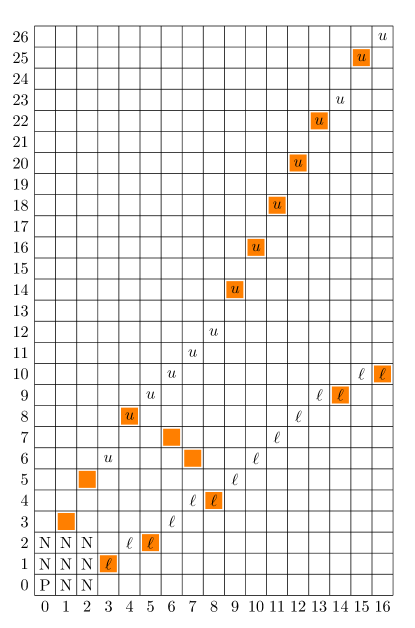
Let and be such that all the altered game states and (described above) are within the box .
We will be computing the game’s P-positions left to right, column by column. By the time we’ve finished a column, we will have computed a finite number of P-positions in that column. All the other positions in that column are N-positions. We compute a column (given that all the ones to its left have been computed) as follows:
We work our way up, starting from row 0. For each cell, if it’s in or we label it as such, and continue. If it’s not, then we compute its label as follows: It’s P if all those in the same column below it are N positions, AND all those in the same row to the left of it are N positions, AND all those diagonally down and to the left are N positions. Otherwise it’s an N position.
The process terminates when we reach row or above AND at least one P position has been found in this column. The process is guaranteed to terminate because for a column the maximum height of a P-position in that column is bounded by .
Let’s consider the simpler case of computing a column (so all of and are strictly to the left of ). A column is called natural if . We know that the column must contain exactly one P-position. The problem is to find it. We work our way up from row 0, looking for that P-position as follows:
If the row we’re in contains only N-positions, and the diagonal of slope 1 down and to the left also contains only N-positions, then this point is the P-position in column .
Say we’re testing a row , using the above method. The only information (about what has been computed so far) needed to do the test is (1) does row already contain a P-position? And also does the diagonal through already contain a P-position?
This information can be captured by two boolean arrays, which we call rowt-1[] and diagt-1[]. rowt-1[] is TRUE if and only if one of the columns to the left of contains a P-position in row . And diagt-1[] is TRUE if and only if the diagonal of slope 1 ending at ) contains a P-position. Once the P-position in column has been computed, the two arrays can be updated to reflect this change going forward. (diagt[] is obtainied by shifting diagt-1[] up by 1, then editing it for the result of the P-position found in column . rowt[] is the same as rowt-1[] except at the position where the new P-position was found.)
We’re going to need to keep track of another thing about these arrays. The variables and are functions of the diagt[]. Specifically is the minimim row such that diagt[] is TRUE, and is the maximum row such that diagt[] is TRUE.
3 Convergence Toward the Natural Wythoff Game
Lemma 1.
After a natural column is computed we know that for all that row is TRUE. And we know that for all that row is FALSE.
Proof.
Consider the first part – for that we must have row TRUE. If the statement is vacuously true. So suppose . Let be the P-position picked in column . We know , because the diagonal through is used, and represents the lowest diagonal used. When searching for the P-position the algorithm rejected . None of those are on a used diagonal. The only explanation for why they were rejected is because those rows are used.
For the second part, for the sake of contradiction, suppose there is a row with and row TRUE. Let be the column containing that P-position, i.e. is a P-position. It immediately follows that the diagonal through is used. But , contradicting the requirement that represent the highest used diagonal. ∎
A column is said to be saturated if diag[] TRUE iff . In this situation the values of and completely characterize the set of diagonals that are used.
Lemma 2 (Saturation Lemma).
There exists a natural column such that and all subsequent columns are saturated.
Proof.
For a column , let be the number of unused diagonals ending at , where . The column is not saturated iff .
Let be a natural column for which we’re about to compute its P-position. Suppose that is unsaturated. There are three cases to consider based on where the P-position in column can reside.
- Case 1:
-
The P-position is at . In this case .
- Case 2:
-
The P-position is at . In this case .
- Case 3:
-
The P-position is at where . In this case .
In Cases 1 or 2 the number of unused diagonals does not change, i.e. . In Case 3 we have . We will show that Case 3 must happen after a finite number of steps. It follows by induction that at some time in the future that . This will prove the lemma.
So our remaining task is to prove that Case 3 must happen eventually. So let’s assume the contrary and try to imagine a scenario where only Cases 1 and 2 occur.
- Observation 1:
-
Case 1 cannot happen twice in a row. Because when it happens row is used and . If it happened twice in a row that row would be used twice.
- Observation 2:
-
When Case 2 happens it creates two unused neighboring rows in the range , because in this case increases by two, introducing the two unused rows in that range.
- Observation 3:
-
Any diagonal that is strictly between and will always remain strictly between them as increases.
Let’s just say for a second that there is exacly one unused diagonal between and . And using observation 2, we have two unused rows between and . We can now compute where these meet. There will a point where the lower of the two unused rows meets the diagonal. And another point where the upper of the two unused rows meets the diagonal.
As we run forward computing column after column, and only Case 1 and Case 2 occur, eventually we get to a time . The point is on an unused diagonal between and . Also, row is not used. So the only thing preventing selection of as the next P-position is the possibility that Case 1 occurs. Okay, so say that happens. Now for the next column Case 1 cannot happen (Observaton 1). So the search for a P-position continues up and before it reaches it will find . Selecting this P-position fills in the previously unused diagonal.
Now we can remove the assumption that there is just one unused diagonal. Because the only thing that can go wrong with the proof above is that the P-position covers some other unused diagonal and fills it in. But this still reduces and makes progress towards the goal.
This completes the proof. ∎
Definition: For any altered Wythoff’s Nim game at time let be the binary string defined by starting with and replacing each FALSE by and each TRUE by .
Definition: The Wythoff Update of a non-empty binary string is obtained from as as follows:
If the first character of is then change that character to a and append to the right end of . Alternatively, if the first character of is then remove it from , and append to the right end of .
Note that the update increases the length of the string by one.

Lemma 3 (String Update Lemma).
Consider and at any time after saturation has occurred. Then the Wythoff Update applied to gives .
Proof.
After saturation, only Cases 1 and 2 occur. So we consider these two cases. The context is that we’ve computed column and have and are now computing column and .
If the leftmost bit of is then Case 1 in the proof holds. Thus . The new P-position is at . Translating these changes to strings, you can see that is obtained from by replacing its leftmost 0 bit with a 1, and adding a 0 to the right end. (This occurs when computing column in Figure 3.)
If the leftmost bit of is this corresponds to Case 2 in the proof. In this case . The fact that causes the leftmost bit of (a 1) to be removed. And the fact that means that two bits are added to the right end of . And a 0 is added to row . And also the new P-position is added to row . So is obtained from by removing the leftmost 1 and appending 01 on the right. (This occurs when computing column in Figure 3.) ∎
4 Properties of the Wythoff String Update Rule
Definition: Let and be bitstrings. We say that and are balanced if they have the same length and the same number of ones.
Lemma 4.
Starting with two arbitrary bitstrings and of the same length, Wythoff updates are applied to both of them producing two sequences of strings and . Then there exists a time when and become balanced.
Proof.
Since the Wythoff update increases the length of a string by one, it follows that for all . For convenience, let and denote the number of zeros and ones in before applying any updates. Define and similarly.
If , the lemma is trivially true. Otherwise, without loss of generality, assume that . Since both strings have the same length, this implies that . Let . We can induct on the value of . Assume that for all , the lemma is true.
By applying the Wythoff update to a string, the number of ones in the string increases by if the first bit is a , and stays the same otherwise. So after applying Wythoff updates, the number of ones in will increase by exactly . Furthermore, since and , there must exist some prefix of with exactly zeros and strictly less than ones. Let the number of ones in be . (Note that the last character of must be a 0.)
Consider the situation after updates of . (This is one update for each 1 in , and two updates for each 0 in , except the last one, for which only one update is done.) The result of these updates is that the number of ones in will have increased by exactly . And . Since the number of ones never decreases after a Wythoff update, the number of ones in after applying updates is at least , and the value of must strictly decrease after a finite number of updates.
If remains positive after these updates, then we can use the induction hypothesis. Otherwise, becomes negative. The number of ones in a string increases by at most with each Wythoff update. So can change by an absolute value of at most with each Wythoff update, and there must have been some point in time when and had the same length and the same number of ones. ∎
Definition: Let be a function on bitstrings, which simultaneously replaces each 0 with 001, and each 1 with 01. For example, . For repeated application of , we write — for example, . Note that applying is equivalent to applying Wythoff updates to a bitstring .
There are several useful facts about when it is applied to a bitstring , which will be useful later. All of them, listed below, can be easily proved inductively.
-
•
If is nonempty, the last character of is a 1, and the first character is a 0.
-
•
No two consecutive characters of are both ones.
-
•
No three consecutive characters of are all zeros.
-
•
There are zeros and ones in .
-
•
The length of is equal to the number of ones in , or algebraically: .
-
•
From the previous two facts, the number of zeros in satisfies .
-
•
It follows that .
-
•
For any prefix of not ending in a zero, there exists a prefix of satisfying . In particular, if is the empty prefix, then is also the empty prefix.
At this point, it will be helpful to introduce visuals for intuition. We represent a bitstring as a curve on a 2-D grid. A 0 corresponds to moving to the right, and a 1 corresponds to moving up. For example, the curve corresponding to 111001 would be drawn:
![[Uncaptioned image]](/html/2408.02851/assets/figures/111001_drawing.png)
By experimentation with small examples, we can observe that the area between two balanced strings appears to stay invariant under applications of . For example, the evolution of 00100111 (in blue) and 11001100 (in red) under two applications of are pictured below. The area between the curves remains equal to throughout.
![[Uncaptioned image]](/html/2408.02851/assets/figures/area_invariant.png)
This motivates the following definitions, which identify each unit of area with a coordinate:
Definition: A unit of area is described by , an ordered pair of integers. is said to be below a string if there exists a prefix of with at most zeros and at least ones. Similarly, is above if there exists a prefix of with at most ones and at least zeros.
Definition: A unit of area is between two balanced strings and , if it is above one of the strings and below the other.
Definition: For balanced bitstrings, the area between and is the number of units of area between and .
The area between and must be finite, since for a unit of area to be below one string and above the other, it must satisfy and . Also, a unit of area cannot simultaneously above and below a string — since if is below , then the shortest prefix with zeros must have at least ones, and so it cannot also be above .
The following two lemmas provide insight into how units of area are transformed by applications of :
Lemma 5.
Let and be balanced bitstrings. If is between and , then is between and .
Proof.
Without loss of generality, suppose that is above and below . First, we show that is below :
-
•
Let be a prefix of with zeros and ones, for some and . Such a prefix must exist by the definition of being below .
will have zeros and ones. Consider the shortest suffix of with zeros. Since there are no two consecutive ones, and the since suffix must have a zero at its end, this suffix can have at most ones. So, removing this suffix from results in a string with zeros and at least ones. So is below .
And a proof that is above :
-
•
The proof is similar to the one above. Let be a prefix of with ones and zeros, for some and .
will have zeros and ones. Consider the shortest suffix of with ones. Since there are no three consecutive zeros, and since the suffix must have ones at both ends, the suffix can have at most zeros. So, removing this suffix from results in a string with at least zeros and ones. So is above .
So is between and .
∎
Lemma 6.
Let and be balanced bitstrings. If is between and , then is between and .
Proof.
Without loss of generality, suppose that is above and below .
Since it is above , there exists a prefix of with ones and zeros, for some , and . If the last character of is not a one, extend its length until its last character is a one. This is possible because the last character of must be a one. By performing this extension, we now have the inequalities and . Now consider — the prefix of satisfying .
The number of ones in is
And the number of zeros in is
So is the prefix we are looking for to prove that is above .
The proof that is below proceeds similarly. Let be a prefix of with zeros and ones, for some , and . Reduce the length of while it ends in a zero. Note that after this modification, the number of ones does not change. Since the number of ones is strictly positive, and cannot start with a 1, the number of zeros must also be positive. And we have and . Let . We can then derive:
And,
So is below , and thus between and .
∎
It’s easy to verify that and are inverses of each other. It follows that is between and if and only if is between and .
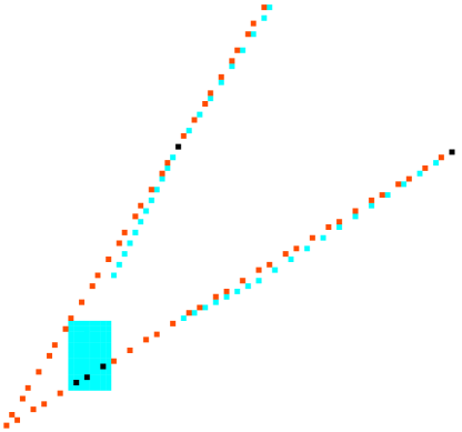
On closer inspection of the pictures, we can see that the area not only remains constant, but that the units of area get more and more separated with each application of .
![[Uncaptioned image]](/html/2408.02851/assets/figures/large_example.png)
A larger example, with more steps of evolution. The curves approach two lines,
differing only by single disjoint units of area.
We make this intuition precise with the notion of a defect:
Definition: For balanced bitstrings and , a defect is an index such that:
-
•
The prefixes of and with length are balanced.
-
•
-
•
-
•
Definition: Two bitstrings and differ by defects if they are balanced, and for every index where , there is a defect either at index or . In other words, every difference between and is a part of a defect.
Visually, a defect is a single isolated unit of area between the two strings. And the strings differ by defects if no two units of area touch each other. We use this visual intuition to motivate the following lemmas:
Lemma 7.
Let and be balanced. Then the following are equivalent:
-
•
For all units of area and between and , and .
-
•
and differ by defects.
And, if they differ by defects, the number of defects is equal to the area between and .
Proof.
Suppose and satisfy the first condition, we prove that they differ by defects. Let be the indices where differs from . The number of such indices must be even, otherwise the number of zeros in one string would be odd while the number of zeros in the other would be even, contradicting the definition of balanced.
If , and trivially differ by defects. Otherwise consider and . The prefix of length is balanced, since that prefix is the same between the two strings. Let and be the number of zeros and ones in this prefix repsectively.
If , then both and would be between and , contradicting the condition above. Similarly, if , then both and would be between and .
So . And if , then , , and would be between and . So all the conditions for index to be a defect hold.
Finally, note that since is a defect, the prefixes of and with length must be balanced. So the prefix with length is balanced, and we can apply the same logic to indices and , and so on, for each and () to show that all indices where and differ are either defects, or come directly after a defect.
Now suppose and differ by defects. We will first show that there is a unit of area between and at if and only if there is a defect at index . One direction is easy — given a defect at index , where there are zeros and ones in the prefix of length , then will be between and .
Now consider any unit of area between and . Without loss of generality, say it is above and below . Since and differ by defects, any time they differ, causing those prefixes to become unbalanced, it gets corrected at the next index. So in any prefix of , and of where , the number of ones in differs from the number of ones in by at most . So must correspond to a prefix of with ones and zeros, and a prefix of with ones and zeros. and only become unbalanced at their defects, so there must be a defect at index .
Now consider the first defect at position , let and be the number of zeros and ones respectively in the prefix of length . There will be a unit of area at . The prefixes of length are unbalanced, and become balanced again at . So the earliest that the next defect can appear is at index , which has strictly more zeros and ones. So the next unit of area must have a strictly greater and coordinate. And extending this reasoning, no two distinct units of area can share a or coordinate.
∎
Lemma 8.
Let as above. Let for be the -th Fibonacci number. Then for , .
Proof.
The proof is by induction, and follows easily from the statement of the lemma. We use .
-
•
For , we can verify that .
-
•
Let , and assume the lemma holds for all . Then, we just need some dense but straightforward computation:
∎
Lemma 9.
Let and be balanced. Then there exists an integer , such that and differ by defects.
Proof.
Let . We will show that for any two distinct units of area and between and , at least one of and is true.
Let and be between and . Assume for sake of contradiction that , and let . From Lemma 6, and are between and iff and are between and . And using the result from Lemma 8, this means that the -coordinates of and differ by
Since , this means that there must be two units of area between and , whose -coordinates differ by at least . But a unit of area can only be between and if its -coordinate ranges from . So these two units of area cannot exist, and no two distinct units of area between and have the same -coordinate.
Similarly, we can assume for sake of contradiction that , and now let . Using the same argument, the corresponding units of area between and would have to have -coordinates differing by
Meaning the -coordinates would have to differ by at least , again a contradiction.
So , and we can apply Lemma 7 to see that and differ by defects.
As a side note, is a very loose bound. Since the difference in coordinates grows on the order of the Fibonacci numbers, the actual number of applications of needed is asymptotically .
∎
Corollary 1 (Convergence).
Given any two bitstrings and of equal length, after applying a finite number of Wythoff updates, they will differ by defects.
Proof.
Apply Wythoff updates until the strings are balanced. Then repeatedly apply (which is equivalent to applying a finite number of Wythoff updates) as prescribed in Lemma 9 until the strings differ by defects. ∎
Corollary 2 (Defect Preservation).
Let and differ by defects. Then and also differ by the same number of defects.
Proof.
From Lemma 7, we know that for any two units of area , either and , or and . Suppose that , then we can see that and . So no two units of area in and share the same or coordinate, and we apply lemma 7 again to see that they differ by defects.
And the number of defects is equal to the area between and . Since the area is preserved, the number of defects is preserved. ∎
5 Asymptotic Equality and Offset
We will now connect the results of the previous section about the evolution of bitstrings under the Wythoff Update to the set of P-positions of the two games.
Given a set of P-positions of a game, let be the same set offset by . That is
Let and be two infinite sets of points in . Let We say that and are asymptotically equal if
It’s not hard to see that asymptotic equivalence defines an equivalence relation on subsets of , which we will denote as .
Theorem 1 (Unique Offset Theorem).
Let be the set of P-positions of an altered Wythoff’s Nim game. Let be the set of P-positions of the natural Wythoff’s Nim game. Then there exists a unique offset such that is asymptotically equal to .
Proof.
By Lemma 2 we know that there is a column in the altered game that is saturated, and all subsequent columns are saturated. The length of the corresponding bitstring at time is , and this increases by one on each step.
For the natural Wythoff’s Nim game at time the length of the bitstring is . So is the amount of “head start” we are going to give the natural game so that the two games align. So we have to define such that
So . (Note that this is not a function of because both and increase by on one each time step.)
As for the value of , Corollary 1 tells us that there is a time when the two games will have bitstrings that just differ by defects. Let in the altered game A. We also need to look at what is happening in the natural game at time . It has a corresponding (where indicates that it is taken from the natural game). So we define . And shifting the altered game up by puts the altered game and the natural game into alignment.
Now as we run both of the games forward, the only points in time when different P-positions are generated for the two games is when a defect is being processed. A defect will cause one of the games to generate a P-position in the lower beam (Case 1 in the proof of Lemma 2), and the other game to generate a P-position in the higher beam (Case 2 in the proof of Lemma 2). Then in the next step, the other bit of the defect is processed, and the roles are reversed.
The bitstrings get longer and longer over time, but the number of defects remains the same. Therefore the density of the defects in the bitstrings goes to zero. It immediately follows that the two sets of P-positions (the translated altered game and the natural game) are asymptotically equal.
We also need to show the uniqueness of the offset . Asymptotic equivalence is is an equivalence relation, and thus satisfies transitivity. So if there are three sets , , and , then and implies .
Suppose that , and also that for two distinct offsets. It follows that . From which we infer by transitivity that:
where is a non-zero integer vector. This implies we can keep moving the elements of the set by , over and over again and continue to have asymptotically equality. It’s clearly impossible because all of the P-positions of lie very close two lines of different slopes. One of the lines must eventually have no overlap with its counterpart in the other set. So the limit in the definition of asymptotic equality will have a value of at most . ∎
5.1 How to Compute the Offset
After experimenting with various types of altered games, we were able to make the following conjecture, which turned out to be true. It will be proven below. Let denote a box of width and height whose lower left corner is .
Theorem 2 (Offset of a Box).
Considered the altered game where and . Then , where is the set of P-positions of the unaltered game of Wythoff’s Nim.
Consider a general altered game . Let be the column that is the last one containing any elements of the altered sets. For this altered game, we can run the algorithm for computing the P-positions described in section 2 of this paper. We run it for each column from to . After we’re done with this process we can examine the situation. We compute three quantities from it.
| The number of rows that have P-positions in them | ||||
| The number of diagonals that have P-positions in them | ||||
With these definitions in mind, we can now state the following theorem.
Theorem 3 (General Offset Theorem).
Let be the P-positions of an altered game of Wythoff’s Nim, where , , and are computed as described above. And let be the P-positions of Wythoff’s Nim. Then .
Proof.
For columns and beyond, one P-position is added. And this P-position has the property that it increases by one the number of diagonals covered, the number of rows covered and the number of colums covered. The same holds for the natural game starting from column .
If we start running the two games at the same time, after computing column the altered game will have diagonals, and the natural game will have diagonals. We want these to be equal, but the number of excess diagonals in the altered game is . Therefore we want to “delay” the start of the altered game (by shifting it to the right) by . With this shift the two games will eventually have exactly the same number of diagonals used. (Note that this offset could be positive or negative.)
To compute the offset required we consider the number of rows covered by the two games. After computing column of the altered game we know that it has used rows. After computing the corresponding column for the natural game (column ) we know that it has used rows. But . This means that going forward the altered game will always have used more rows than the natural game. (This of course could be positive or negative.)
So let’s skip ahead in time to a moment when the two games bitstrings differ by defects. We’re going to consider the two values of from section 3 of the paper. Let be its value in the altered game at this time and let be its value in the natural game at this time. All the rows of each game below their respective s are used. And as for the rows above and respectively, there are the same number of rows used in both games. Therefore we know that . Therefore , and this is how much we have to shift up the altered game to align them. ∎
6 Final Remarks
Linear Nimhoff is a class of two-pile Nim games defined by listing a set of rules. Each rule is described by a pair of non-negative integers . Such a rule allows the player to move by converting a pair of pile sizes to , where is a positive integer, so long as the latter vector is non-negative. Linear Nimhoff was defined by Friedman et. al. [2], extending the work of Larsson [4]. Using this notation Wythoff’s Nim is Linear Nimhoff with this rule set: .
It is natural to ask how other games in this class behave when altered. That is, will the phenomena that we observe in Wythoff’s Nim also occur in other Linear Nimhoff games? We can summarize our experimental results as follows:
-
1.
We were unable to observe the phenomenon of defects in any other game. That is, we looked for another game where the pattern of P-positions in the altered game gets closer and closer to the un-altered game as we move to larger and larger coordinates. But we never found this in any game other than Wythoff’s Nim.
-
2.
On the other hand, the overall geometrical structure of the game does not seem to be changed when alterations are applied. So for example if the original game has beams along roughly straight lines (these are the strict class of games as defined in [2]) then any finite alteration asymptotically preserves the same lines.
To illustrate the first point, consider the Linear Nimhoff game defined by this set of rules, which differs very slightly from those of Wythoff’s Nim: . We have proven [3] that the P-positions are comprised of two linear beams defined by the sets and . Where
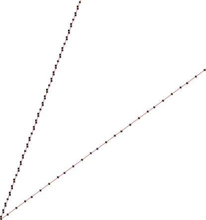
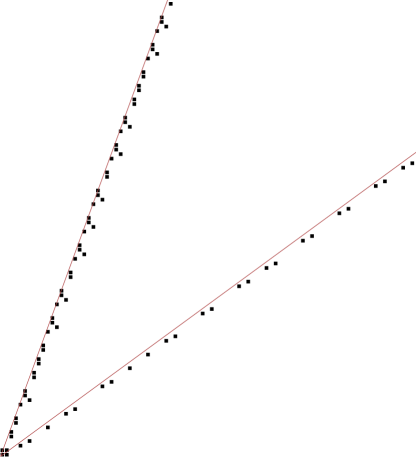
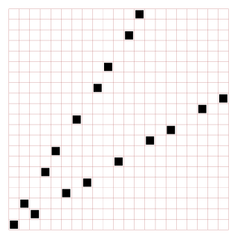
Figure 6 shows the behavior of this game with a small alteration. The structure of the upper beam of the altered game remains entirely different from that of the unaltered game, as far as we’ve computed it.
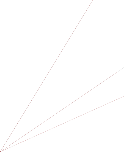
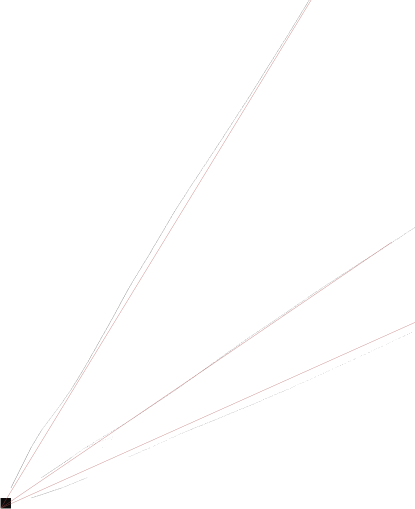
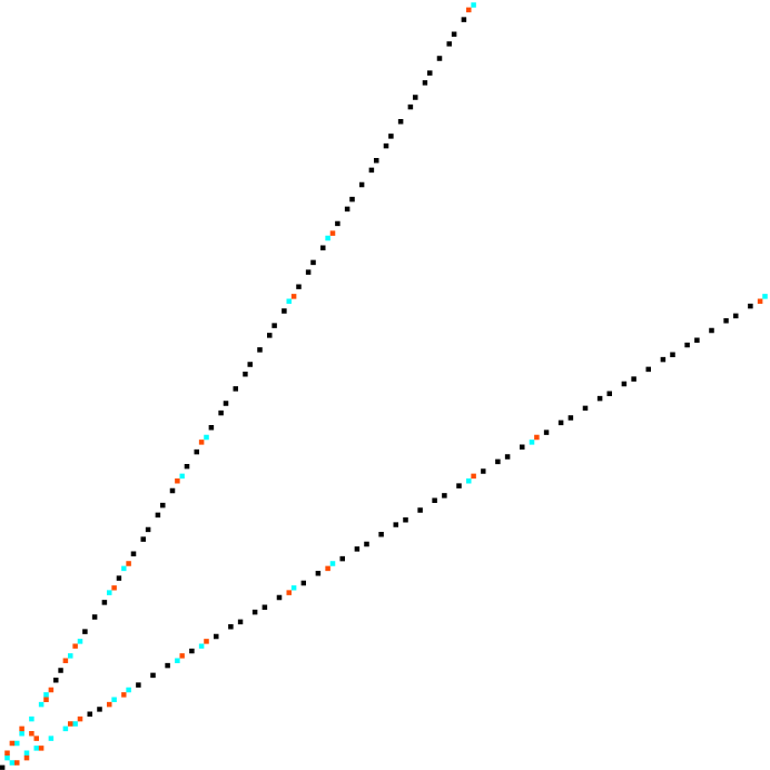
The second point is illustrated in Figure 7. Although initially different, eventually the three beams of P-positions in the altered game conform to the slopes of the corresponding beams in the un-altered game.
References
- [1] E. Duchêne, A. S. Fraenkel, V. Gurvich, N. B. Ho, C. Kimberling, and U. Larsson, Wythoff visions, in Games of No Chance 5, U. Larson, ed., Cambridge University Press, Cambridge, UK, 2017, pp. 35–87.
- [2] E. Friedman, S. M. Garrabrant, I. K. Phipps-Morgan, A. S. Landsbereg, and U. Larsson, Geometric analysis of a generaiized wythoff game, in Games of No Chance 5, U. Larson, ed., Cambridge University Press, Cambridge, UK, 2017, pp. 343–372.
- [3] M. Hu, Exploring variations of wythoff nim, Tech. Rep. CMU-CS-24-119, Carnegie Mellon University, Department of Computer Science, May 2024.
- [4] U. Larsson, A generalized diagonal wythoff nim. https://arxiv.org/abs/1005.1555, 2010.
- [5] W. A. Wythoff, A modification of the game of nim, Nieuw Arch. Wisk, 7 (1907), pp. 199–202.