Randomized quasi-Monte Carlo methods for risk-averse stochastic optimization

Abstract

We establish epigraphical and uniform laws of large numbers for sample-based approximations of law invariant risk functionals. These sample-based approximation schemes include Monte Carlo (MC) and certain randomized quasi-Monte Carlo integration (RQMC) methods, such as scrambled net integration. Our results can be applied to the approximation of risk-averse stochastic programs and risk-averse stochastic variational inequalities. Our numerical simulations empirically demonstrate that RQMC approaches based on scrambled Sobol’ sequences can yield smaller bias and root mean square error than MC methods for risk-averse optimization.

AMS subject classifications. 90C15, 90C59, 65C05

1 Introduction

We consider the risk-averse stochastic optimization problem

$$\min_{x\in X}\rho(F(x,\xi)),$$ (1)

where $X$ is a potentially infinite dimensional decision space, $\Omega$ and $\Xi$ are sample spaces, and $\xi:\Omega\to\Xi$ is a random element. The real-valued function $F$ is defined on $X\times\Xi$ and the real-valued, law invariant risk measure $\rho$ is defined on the Lebesgue space $\mathcal{L}^{p}(\Omega)$ with $p\in[1,+\infty)$.

Two common challenges arise when trying to solve (1) in practice. First, knowledge of the distribution of $\xi$ may be incomplete. For instance, only samples of $\xi$ may be available. Second, the approximation of high-dimensional integrals is computationally intractable. One way to address these issues is to construct sample-based approximations of (1) and solve them instead. Sample average approximation—a Monte Carlo (MC) sample-based approach—is a common approach used to generate consistent approximations to (1) [11, 25]. However, randomized quasi-Monte Carlo (RQMC) can have superior performance in terms of accuracy and variance reduction. Consequently, there is interest in analyzing the effectiveness of methods such as RQMC sampling in the context of stochastic programming.

For the risk-neutral case, the epiconsistency of RQMC-based approximations of (1) is demonstrated in [12]. The numerical experiments in [12] suggest favorable performance of the RQMC sample-based approach compared to MC sampling when applied to risk-neutral stochastic programs. A similar analysis has been conducted for approximation schemes based on quasi-Monte Carlo (QMC) sampling in [22]. Furthermore, [8] provides consistency results for a general class of approximation schemes in the risk-neutral case. These schemes approximate the distribution of $\xi$ using auxiliary distributions. The auxiliary distributions are required to meaningfully approximate the distribution of $\xi$ with respect to specific integrals. The authors of [8] demonstrate that these schemes yield epiconsistent approximations.

Some problems cannot be appropriately modeled with risk-neutral formulations. For instance, portfolio optimization often requires a risk-averse model to avoid potentially detrimental losses. For the risk-averse case, the epiconsistency the MC sample-based approach has been demonstrated in [25]. Moreover, a central limit theorem for MC sample-based composite risk functionals is established in [5].

Our main contribution lies in demonstrating the almost sure epiconvergence and uniform convergence of a class of sample-based approximation schemes for composite risk functionals beyond MC sample-based approaches. In more detail, let $\Theta$ be a sample space and for each $x\in X$, let $F_{x}(\cdot)$ denote the measurable map $\xi\mapsto F(x,\xi)$ on $\Xi$. For a random variable $Z:\Xi\to\mathbb{R}$ and a probability measure $\nu$ on $\Xi$, let $\nu\circ Z^{-1}$ denote the corresponding pushforward measure. Roughly speaking and omitting technical considerations, for suitable random sequences of probability measures $(\nu_{N,\theta})_{N\in\mathbb{N}}$ indexed by $\theta\in\Theta$, we demonstrate the epiconvergence and uniform convergence of

$$x\mapsto\rho(\nu_{N,\theta}\circ F_{x}^{-1})$$ (2)

towards

$$x\mapsto\rho(F_{x}(\xi)).$$ (3)

In the spirit of a strong law of large numbers (SLLN), we require the sequence of probability measures $(\nu_{N,\theta})_{N\in\mathbb{N}}$ to yield consistent approximations of risk functionals as $N\to\infty$. More specifically, we demonstrate that as long as for all random variables $Z\colon\Xi\to\mathbb{R}$ such that $Z\circ\xi\in\mathcal{L}^{q}(\Omega)$ with $q\geq p$, and

$$\rho(\nu_{N,\theta}\circ Z^{-1})\to\rho(Z(\xi))\quad\quad\text{as}\quad N\to\infty\quad\text{for almost all}\quad\theta\in\Theta,$$ (4)

the sample-based composite risk functions (2) yield epiconsistent approximations to (3). The condition (4) is canonically satisfied for MC sample-based approximations. For these approximations, our epiconsistency results coincide with those in [25]. We further demonstrate that (4) is satisfied for certain RQMC-based schemes, notably those given by scrambled digital nets. Our verification leverages the SLLN recently established in [21]. When combined with standard properties of epiconvergence and compactness of the decision space $X$, our epigraphical law of large numbers provides conditions sufficient for almost sure consistency of the optimal value of

$$\min_{x\in X}\,\rho(\nu_{N,\theta}\circ F_{x}^{-1})$$

towards that of (1).

Furthermore, we provide conditions sufficient for the uniform convergence of (2) towards (3). These sufficient conditions are also based on a SLLN, but are more stringent than (4). For MC sample-based approximations, this uniform law of large numbers coincides with the standard one for real-valued Carathéodory functions. We use this uniform SLLN to demonstrate consistency of the sample-based approximations to risk-averse stochastic variational inequalities of the form

$$0\in\Big{[}\rho_{1}(F^{1}_{x}(\xi)),\ldots,\rho_{r}(F^{r}_{x}(\xi))\Big{]}+{\partial\psi(x)},$$ (5)

where $\psi\colon\mathbb{R}^{r}\to(-\infty,+\infty]$ is proper, closed, and convex with compact domain $X$, and $\rho_{j}$, $j=1,\ldots,r$, are real-valued, law invariant risk measures and $F_{x}^{j}$, $j=1,\ldots,r$, are maps with properties related to those of $F_{x}$. Here $\partial\psi(x)$ is the subdifferential of $\psi$ at $x\in\mathbb{R}^{r}$. An instance of (5) is considered in [4], where all $\rho_{j}$ equal the conditional value-at-risk, and $\psi$ is the indicator function of a nonempty, convex, compact set $X$. The variational inequality in (5) is an instance of the distributionally robust stochastic variational inequalities considered in [27].

Overview

After introducing notation in Section 2, we discuss conditions sufficient for consistent approximations of law invariant risk functionals and provide examples in Section 3. In Section 4, we establish conditions sufficient for the almost sure epiconvergence of composite risk functionals. Subsequently, we give conditions sufficient for a uniform law of large numbers. We apply this result to risk-averse stochastic variational inequalities. Finally, we provide numerical experiments comparing MC and RQMC sample-based methods for risk-averse stochastic programs in terms of the root mean square error (RMSE) and bias in Section 6.

2 Notation and Preliminaries

Throughout the text, let $(\Omega,\mathcal{F},P)$ be a probability space, let $\Xi$ be a separable metric space equipped with its Borel $\sigma$-algebra, let $\xi\colon\Omega\to\Xi$ be a random element, let $p\in[1,+\infty)$ and $\varepsilon\geq 0$ be scalars. We impose additional assumptions on these objects as needed. Moreover, let $\lambda$ denote the Lebesgue measure on $[0,1]^{d}$. With a slight abuse of notation, we use $\xi$ to denote both the random element introduced above and deterministic elements in $\Xi$.

Next, we introduce basic terminology and notation. We denote the uniform distribution on a set $C\subset\mathbb{R}^{d}$ by $\text{Uniform}(C)$. We call $(\Omega,\mathcal{F},P)$ nonatomic if there exists a random variable $U:(\Omega,\mathcal{F},P)\to(0,1)$ such that $U\sim\text{Uniform}(0,1)$. We denote the space of $p$-integrable random variables on $(\Omega,\mathcal{F},P)$ by $\mathcal{L}^{p}(\Omega,\mathcal{F},P)$, or simply by $\mathcal{L}^{p}(\Omega)$. A functional $\rho:\mathcal{L}^{p}(\Omega,\mathcal{F},P)\to(-\infty,+\infty]$ is called law invariant (with respect to $P$) if for each $Y,Z\in\mathcal{L}^{p}(\Omega,\mathcal{F},P)$ with the same distribution, we have $\rho(Y)=\rho(Z)$ [26, Def. 6.26]. A risk measure $\rho\colon\mathcal{L}^{p}(\Omega,\mathcal{F},P)\to(-\infty,+\infty]$ is said to be convex if it is a convex, monotone, and translation equivariant function [26, Def. 6.4]. Let $V$ be a nonempty set. The indicator function $\mathbb{1}_{V_{0}}\colon V\to\mathbb{R}$ of a subset $V_{0}\subset V$ is defined by $\mathbb{1}_{V_{0}}(v)=1$ if $v\in V_{0}$ and $\mathbb{1}_{V_{0}}(v)=0$ otherwise. Let $\mu,\mu_{1},\mu_{2},\ldots$ be probability measures, and $Z,Z_{1},Z_{2},\ldots$ be random variables. We denote the weak convergence of the sequence $(\mu_{n})_{n\in\mathbb{N}}$ to $\mu$, and respectively, $(Z_{n})_{n\in\mathbb{N}}$ to $Z$, by $\mu_{n}\xrightarrow{w}\mu$ and $Z_{n}\xrightarrow{w}Z$ as $n\to\infty$. If not specified otherwise, metric spaces $\Upsilon$ are equipped with their Borel $\sigma$-algebra $\mathcal{B}(\Upsilon)$. For a metric space $X$, a function $G\colon X\times\Upsilon\to\mathbb{R}$ is called a Carathéodory function if $G(x,\cdot)$ is $\mathcal{B}(\Upsilon)$-$\mathcal{B}(\mathbb{R})$-measurable for each $x\in X$, and $G(\cdot,\upsilon)$ is continuous for every $\upsilon\in\Upsilon$. A function $G\colon X\times\Upsilon\to(-\infty,+\infty]$ is called random lower semicontinuous if the epigraphical multifunction $\upsilon\mapsto\{(x,t)\in X\times\mathbb{R}\colon t\geq G(x,\upsilon)\}$ is closed-valued and measurable. For functions $f$, $f_{n}\colon X\to(-\infty,+\infty]$ epiconvergence of $(f_{n})_{n\in\mathbb{N}}$ to $f$ as $n\to\infty$ means that (i) for all sequences $(x_{n})_{n\in\mathbb{N}}$ and points $x\in X$ with $x_{n}\to x$ as $n\to\infty$, $\liminf_{n\to\infty}\,f_{n}(x_{n})\geq f(x)$, and (ii) for each $x\in X$, there exists a sequence $(x_{n})_{n\in\mathbb{N}}$ with $x_{n}\to x$ as $n\to\infty$ such that $\limsup_{n\to\infty}\,f_{n}(x_{n})\leq f(x)$. For a real-valued random variable $Z$, let $H[Z]:(0,1)\to\mathbb{R}$ denote the quantile function associated with the distribution of $Z$. For a probability distribution $Q$ on $\mathbb{R}$, let $H_{Q}(\cdot)$ indicate the corresponding quantile function.

Remark 1.

If $(\Omega,\mathcal{F},P)$ is nonatomic, then for each probability distribution $Q$ on $\mathbb{R}$ there exists a random variable defined on $(\Omega,\mathcal{F},P)$ with distribution $Q$. Indeed, by definition, nonatomicness guarantees the existence of a random variable $U$ defined on $(\Omega,\mathcal{F},P)$ with $U\sim\text{Uniform}(0,1)$. Since $H_{Q}$ has distribution $Q$, we obtain

$$H_{Q}(U)\sim Q.$$

The above remark justifies viewing law invariant risk measures defined on $\mathcal{L}^{p}(\Omega,\mathcal{F},P)$ as functions of probability distributions on $\mathbb{R}$ with finite $p$th moment, provided that $(\Omega,\mathcal{F},P)$ is nonatomic.

3 Consistent Approximations of Law Invariant Functionals

Empirical distributions have been shown to yield consistent approximations of risk functionals [2, 23, 25]. The main result of this section, Theorem 1 presented below, generalizes this result to a broader class of distributions. Notably, we use Theorem 1 to demonstrate that MC and scrambled net integration consistently approximate risk functionals defined on Lebesgue spaces.

Theorem 1 (Consistent Approximations of Law Invariant Functionals).

Let $(\Omega,\mathcal{F},P)$ be nonatomic. Consider a law invariant, continuous functional $\rho:\mathcal{L}^{p}(\Omega,\mathcal{F},P)\to\mathbb{R}$. Let $\mu,\mu_{1},\mu_{2},\ldots$ be probability measures on $\mathbb{R}$, and let $\int_{\mathbb{R}}\lvert t\rvert^{p}\,\,\mathrm{d}\mu(t)<\infty$. Further, suppose that

$$\mu_{N}\xrightarrow{w}\mu\quad\text{and}\quad\int_{\mathbb{R}}\lvert t\rvert^{p}\,\mathrm{d}\mu_{N}(t)\to\int_{\mathbb{R}}\lvert t\rvert^{p}\,\mathrm{d}\mu(t)$$ (6)

as $N\to\infty$. Then

$$\rho(\mu_{N})\to\rho(\mu)\;\;\textnormal{as}\;\;N\to\infty.$$

Proof.

Theorem 1.4.1 in [23] yields

$$\int_{(0,1)}\lvert H_{\mu_{N}}(t)-H_{\mu}(t)\rvert^{p}\,\mathrm{d}t\to 0\;\;\textnormal{as}\;\;N\to\infty.$$

Thus, for $U\sim\text{Uniform}(0,1)$ defined on $(\Omega,\mathcal{F},P)$, $H_{\mu_{N}}(U)$ converges to $H_{\mu}(U)$ in $\mathcal{L}^{p}(\Omega)$. Law invariance and continuity of $\rho$ yield the result (see Remark 1). ∎

Empirical means defined by standard MC sampling satisfy a SLLN and the corresponding empirical distributions converge weakly, under mild assumptions. These facts can be used to verify the convergence statements in (6) for MC sampling. More generally, the conditions in (6) hold for all measures generated by a sampling method that satisfies a SLLN-type condition. We formulate this SLLN-type condition in the assumption below and demonstrate how it can be used to verify (6) in the next lemma.

Assumption 1.

Let $(\xi^{i})_{i\in\mathbb{N}}$ be a sequence of $\Xi$-valued random elements defined on a probability space $(\Theta,\mathcal{A},\mathbb{P})$. For each random variable $\vartheta:\Xi\to\mathbb{R}$ with $\vartheta\circ\xi\in\mathcal{L}^{1+\varepsilon/p}(\Omega)$, we have

$$\frac{1}{N}\sum_{i=1}^{N}\vartheta(\xi^{i}(\theta))\to\int_{\Omega}\vartheta\circ\xi\,\mathrm{d}P\;\;\textnormal{as}\;\;N\to\infty\quad\text{for }\mathbb{P}\text{-almost all }\theta\in\Theta.$$

Let Assumption 1 hold. For $\theta\in\Theta$ and $N\in\mathbb{N}$, let us define the probability measure $\nu_{N,\theta}$ on $\Xi$ by

$$\nu_{N,\theta}(B)\coloneqq\frac{1}{N}\sum_{i=1}^{N}\mathbb{1}_{\xi^{i}(\theta)}(B)$$ (7)

for each $B\in\mathcal{B}(\Xi)$. We show that Assumption 1 allows us to verify the conditions in (6). In a later section, we also reuse Assumption 1 to formulate our uniform law of large numbers.

Lemma 1.

Let Assumption 1 hold, and let $Z\colon\Xi\to\mathbb{R}$ be a random variable with $Z\circ\xi\in\mathcal{L}^{p+\varepsilon}(\Omega)$. Let $\mu_{N,\theta}\coloneqq\nu_{N,\theta}\circ Z^{-1}$ and let $\mu$ be the distribution of $Z\circ\xi$. Then $\mu_{N,\theta}\xrightarrow{w}\mu$ and $\int_{\mathbb{R}}\lvert t\rvert^{p}\,\mathrm{d}\mu_{N,\theta}(t)\to\int_{\mathbb{R}}\lvert t\rvert^{p}\,\mathrm{d}\mu(t)$ for $\mathbb{P}$-almost all $\theta\in\Theta$.

Proof.

First, we show that $\mu_{N,\theta}\xrightarrow{w}\mu$ as $N\to\infty$ for $\mathbb{P}$-almost all $\theta\in\Theta$. We denote the countable set of continuous, bounded functions $W:\mathbb{R}\to\mathbb{R}$ given in Corollary 2.2.6 in [3] by $\mathcal{W}$. For each $W\in\mathcal{W}$, $(W\circ Z)\circ\xi\in\mathcal{L}^{\infty}(\Omega)$. Thus, for each $W\in\mathcal{W}$, Assumption 1 yields the existence of a $\mathbb{P}$-full set $\Theta_{W}$ such that

$$\int_{\Xi}W\circ Z\,\mathrm{d}\nu_{N,\theta}=\frac{1}{N}\sum_{i=1}^{N}W(Z(\xi^{i}(\theta))\to\int_{\Omega}(W\circ Z)\circ\xi\,\mathrm{d}P\;\;\textnormal{as}\;\;N\to\infty$$ (8)

for each $\theta\in\Theta_{W}$. The set $\Theta_{1}\coloneqq\bigcap_{W\in\mathcal{W}}\Theta_{W}$ is $\mathbb{P}$-full since it is a countable intersection of $\mathbb{P}$-full sets. Now, for each $\theta\in\Theta_{1}$ and $W\in\mathcal{W}$, a change of variables on both sides of (8) yields

$$\int_{\mathbb{R}}W\,\mathrm{d}\mu_{N,\theta}(t)\to\int_{\mathbb{R}}W\,\mathrm{d}\mu(t)\;\;\textnormal{as}\;\;N\to\infty.$$

Combined with Corollary 2.2.6 in [3], we have $\mu_{N,\theta}\xrightarrow{w}\mu$ as $N\to\infty$ for all $\theta\in\Theta_{1}$. Since $Z\circ\xi\in\mathcal{L}^{p+\varepsilon}(\Omega)$, we have $|Z(\xi)|^{p}\in\mathcal{L}^{1+\varepsilon/p}(\Omega)$. Using Assumption 1, we also obtain the existence of a $\mathbb{P}$-full set $\Theta_{2}$ such that

$$\int_{\mathbb{R}}\lvert t\rvert^{p}\,\mathrm{d}\mu_{N,\theta}(t)=\int_{\Xi}\lvert Z\rvert^{p}\,\mathrm{d}\nu_{N,\theta}\to\int_{\Xi}\lvert Z(\xi)\rvert^{p}\,\mathrm{d}P=\int_{\mathbb{R}}\lvert t\rvert^{p}\,\mathrm{d}\mu(t)\;\;\textnormal{as}\;\;N\to\infty$$

for all $\theta\in\Theta_{2}$. ∎

3.1 Examples

We use Theorem 1 to derive consistency results for approximations of risk functionals generated by MC and QMC sampling, scrambled net integration, and Latin hypercube sampling. Importantly, these examples serve as justification for a pivotal assumption, Assumption 4, used to formulate our epigraphical law of large numbers in later sections.

For the examples below we require the following assumption.

Assumption 2.

The probability space $(\Omega,\mathcal{F},P)$ is nonatomic, and the risk measure $\rho:\mathcal{L}^{p}(\Omega,\mathcal{F},P)\to\mathbb{R}$ is law invariant and continuous.

First, we demonstrate that Theorem 1 is compatible with classical MC sampling.

Example 1 (MC-based measures).

Let $Y\in\mathcal{L}^{p}(\Omega,\mathcal{F},P)$. Let $Y_{1},Y_{2},\ldots$ be independent, identically distributed (iid) random variables defined on a probability space $(\Theta,\mathcal{A},\mathbb{P})$ with $Y_{1}\sim Y$. We define the empirical distribution corresponding to $Y_{1},Y_{2},\ldots,Y_{N}$ by

$$\pi_{N,\theta}(B)\coloneqq\frac{1}{N}\sum_{i=1}^{N}\mathbb{1}_{Y_{i}(\theta)}(B)$$

for each $B\in\mathcal{B}(\mathbb{R})$ and $\theta\in\Theta$. Let Assumption 2 be satisfied. Using the SLLN and the almost sure weak convergence of empirical distributions, we find that

$$\rho(\pi_{N,\theta})\to\rho(Y)\;\;\textnormal{as}\;\;N\to\infty\quad\text{for }\mathbb{P}\text{-almost all }\theta\in\Theta.$$

This convergence statement has already been established in [23, pp. 32–33], Theorem 2.1 in [25], and Theorem 9.65 in [26].

It is worth noting that MC sampling can also be examined using Lemma 1. The resulting formulation is consistent with that of Assumption 4 in the next section.

Example 2 (MC-based measures, continued).

Let $(\xi^{i})_{i\in\mathbb{N}}$ be a sequence of iid random elements on $(\Theta,\mathcal{A},\mathbb{P})$ with $\xi^{1}\sim\xi$. Let Assumption 2 be satisfied. Owing to the SLLN, Assumption 1 is met for $\varepsilon=0$. Now, Lemmas 1 and 1 ensure that for each random variable $Z\colon\Xi\to\mathbb{R}$ with $Z\circ\xi\in\mathcal{L}^{p}(\Omega)$, we have

$$\rho(\nu_{N,\theta}\circ Z^{-1})\to\rho(Z(\xi))\;\;\textnormal{as}\;\;N\to\infty\quad\text{for }\mathbb{P}\text{-almost all }\theta\in\Theta,$$

where $\nu_{N,\theta}$ as in (7) with iid $(\xi^{i})_{i\in\mathbb{N}}$.

The next example is in the spirit of QMC methods. QMC methods typically approximate the Lebesgue measure on the unit cube using discrete measures defined by deterministically generated points, also referred to as low-discrepancy sequences. Roughly speaking, low-discrepancy sequences are designed to cover the integration domain evenly. As a consequence, these deterministic measures weakly converge to the Lebesgue measure. While QMC methods avoid the potentially unfavorable clustering of points that can occur with the vanilla MC method, they typically require some smoothness assumptions on the integrand. We demonstrate a consistency result for weakly convergent measures in the context of risk measures, provided that a smoothness condition is satisfied.

Example 3 (Weakly convergent measures).

Let $\nu$ be a probability measure on $(\Xi,\mathcal{B}(\Xi))$. Suppose $Z$ is a real, $\nu$-almost surely continuous, and bounded random variable defined on $(\Xi,\mathcal{B}(\Xi),\nu)$. Let $\nu_{1},\nu_{2},\ldots$ be probability measures with

$$\nu_{N}\xrightarrow{w}\nu\;\;\textnormal{as}\;\;N\to\infty.$$

We have

$$\rho(\nu_{N}\circ Z^{-1})\to\rho(\nu\circ Z^{-1})\;\;\textnormal{as}\;\;N\to\infty.$$

Let us verify this assertion. Owing to the Continuous Mapping Theorem (see Theorem 13.25 in [10]), we have

$$\nu_{N}\circ Z^{-1}\xrightarrow{w}\nu\circ Z^{-1}\;\;\textnormal{as}\;\;N\to\infty.$$

Since $\lvert Z\rvert^{p}$ is $\nu$-almost surely continuous and bounded, we obtain

$$\lim_{N\to\infty}\int_{\Xi}\lvert Z_{N}\rvert^{p}\,\mathrm{d}\nu_{N}=\int_{\Xi}\lvert Z\rvert^{p}\,\mathrm{d}\nu$$

(see Corollary 2.2.10 in [3]). Now, Theorem 1 implies the assertion.

Many RQMC methods randomize deterministic, low-discrepancy points in a way that guarantees uniform distribution of the randomized points while maintaining their low-discrepancy property. In the next example, we consider measures that are obtained by randomizing digital nets on $[0,1]^{d}$ with a uniform nested scramble [21]. Notably, the uniform nested scramble can be used to randomize Sobol’ sequences, which are $(t,d)$-sequences in base $2$ (see Definition 3.2 in [21]).

Example 4 (Scrambled Net Integration).

Let us give details on the RQMC methods considered in this example. Let $(y^{i})_{i\in\mathbb{N}}\subset[0,1]^{d}$ be a $(t,d)$-sequence in integer base $b\geq 2$ (see Definition 3.2 in [21]), where $t\geq 0$ is an integer. Moreover, suppose that the maximum gain coefficient of the sequence is bounded by a finite constant. Let the sequence $(\xi^{i})_{i\in\mathbb{N}}$ of random vectors be obtained through randomization of the sequence $(y^{i})_{i\in\mathbb{N}}$ using the method described in [20]. The random vectors $\xi^{1},\xi^{2},\ldots$ are defined on a probability space $(\Theta,\mathcal{A},\mathbb{P})$, and uniformly distributed on $[0,1]^{d}$, but are not independent. Let $q\in(1,+\infty]$. Theorem 5.3 in [21] ensures that for each $\vartheta\in\mathcal{L}^{q}[0,1]^{d}$, we have

$$\frac{1}{N}\sum_{i=1}^{N}\vartheta(\xi^{i}(\theta))\to\int_{[0,1]^{d}}\vartheta\,\mathrm{d}\lambda\;\;\textnormal{as}\;\;N\to\infty\quad\text{for }\mathbb{P}\text{-almost all }\theta\in\Theta.$$

Let the probability measure $\nu_{N,\theta}$ be as in (7), with the sequence $(\xi^{i})_{i\in\mathbb{N}}$ as described above. We consider $\varepsilon>0$ and $q=1+\varepsilon/p$. Let $Z\in\mathcal{L}^{p+\varepsilon}[0,1]^{d}$ and let $\xi\sim\text{Uniform}[0,1]^{d}$. Then, the above SLLN, and Lemmas 1 and 1 with $\Xi=[0,1]^{d}$ yield

$$\rho(\nu_{N,\theta}\circ Z^{-1})\to\rho(Z(\xi))\;\;\textnormal{as}\;\;N\to\infty\quad\text{for }\mathbb{P}\text{-almost all }\theta\in\Theta.$$

Next, we demonstrate consistent estimation of risk functionals via Latin hypercube sampling, which is a popular variance reduction scheme used in stochastic programming.

Example 5 (Latin hypercube sampling).

Let the sequence $(\xi^{i})_{i\in\mathbb{N}}d$ of random vectors be obtained through Latin hypercube sampling as described in Section 1 in [14] (see also Section 5.5.1 in [26]). The random vectors $\xi^{1},\xi^{2},\ldots$ are defined on a probability space $(\Theta,\mathcal{A},\mathbb{P})$, and uniformly distributed on $[0,1]^{d}$, but are not independent. Then, Theorem 3 in [14] ensures that for each $\vartheta\in\mathcal{L}^{2}[0,1]^{d}$, we have

$$\frac{1}{N}\sum_{i=1}^{N}\vartheta(\xi^{i}(\theta))\to\int_{[0,1]^{d}}\vartheta\,\mathrm{d}\lambda\;\;\textnormal{as}\;\;N\to\infty\quad\text{for }\mathbb{P}\text{-almost all }\theta\in\Theta.$$

Let Assumption 2 be satisfied. Moreover, let the probability measure $\nu_{N,\theta}$ be as in (7), where $(\xi^{i})_{i\in\mathbb{N}}$ is generated using Latin hypercube sampling. Suppose that $\xi\sim\text{Uniform}[0,1]^{d}$. Then, the above SLLN and Lemmas 1 and 1 with $\Xi=[0,1]^{d}$ ensure that for each random variable $Z\colon[0,1]^{d}\to\mathbb{R}$ with $Z\circ\xi\in\mathcal{L}^{2p}(\Omega)$, we have

$$\rho(\nu_{N,\theta}\circ Z^{-1})\to\rho(Z(\xi))\;\;\textnormal{as}\;\;N\to\infty\quad\text{for }\mathbb{P}\text{-almost all }\theta\in\Theta.$$

4 Epiconvergence of Approximations to Composite Risk Functionals

In this section, we establish our main result, an almost sure epiconvergence result for composite risk functionals under consistent pointwise approximations. Our epiconvergence result is based on two technical assumptions. The first assumption is based on the consistency framework developed in [25]. The second assumption can be viewed as a SLLN, which is satisfied for probability measures generated by MC sampling or scrambled net integration.

Assumption 3.

1. The metric space $X$ is separable, and $(\Omega,\mathcal{F},P)$ is complete and nonatomic.

2. The map $F:X\times\Xi\to[0,+\infty)$ is random lower semicontinuous.

3. For every $x\in X$, the random variable $F_{x}(\xi)\coloneqq F(x,\xi)$ is in $\mathcal{L}^{p+\varepsilon}(\Omega,\mathcal{F},P)$.

4. The risk measure $\rho\colon\mathcal{L}^{p}(\Omega,\mathcal{F},P)\to\mathbb{R}$ is convex, and law invariant.

The next assumption formulates a SLLN-type consistency condition, inspired by the examples considered in Section 3.1.

Assumption 4.

Let $(\Theta,\mathcal{A},\mathbb{P})$ be a probability space. For each $\theta\in\Theta$, $(\nu_{N,\theta})_{N\in\mathbb{N}}$ is a sequence of probability measures on $(\Xi,\mathcal{B}(\Xi))$. For each random variable $Z:\Xi\to\mathbb{R}$ with $Z\circ\xi\in\mathcal{L}^{p+\varepsilon}(\Omega,\mathcal{F},P)$, we have

$$\lim_{N\to\infty}\rho(\nu_{N,\theta}\circ Z^{-1})=\rho(Z(\xi))\quad\text{for }\mathbb{P}\text{-almost all }\theta\in\Theta.$$ (9)

Probability measures obtained through MC sampling satisfy Assumption 4 with $\varepsilon=0$ (see Example 1). Moreover, measures derived from scrambled net integration satisfy Assumption 4 with $\varepsilon>0$ (see Example 4).

We now formulate the main result of this section.

Theorem 2 (Epiconvergence of Approximations to Risk Functionals).

Let Assumptions 4 and 3 be satisfied. Then, the sequence of functions

$$x\mapsto\rho(\nu_{N,\theta}\circ F_{x}^{-1})$$

epiconverges to

$$x\mapsto\rho(F_{x}(\xi))$$

for $\mathbb{P}$-almost every $\theta\in\Theta$.

Before we present our proof of Theorem 2, we state some useful facts and introduce notation. For two random variables $V$ and $W$ defined on the same probability space, we have

$$V\geq W\quad\text{almost surely}\quad\text{implies}\quad H[V](t)\geq H[W](t)\quad\text{for all }\quad t\in(0,1).$$ (10)

Moreover, for each $\alpha\in\mathbb{R}$ we have

$$H[V+\alpha](t)=H[V](t)+\alpha\quad\text{for all}\quad t\in(0,1).$$ (11)

For each $x\in X$, let $H_{N,\theta}[F_{x}]:(0,1)\to\mathbb{R}$ denote the quantile function corresponding to the distribution $\nu_{N,\theta}\circ F_{x}^{-1}$. By the reasoning given in Remark 1, we have

$$\rho(\nu_{N,\theta}\circ F_{x}^{-1})=\rho(H_{N,\theta}[F_{x}](U))\quad\text{for each $x\in X$},$$

where $U$ is a random variable on $\Omega$ with $U\sim\text{Uniform}(0,1)$. For the sake of brevity, in the proof below, we denote the random variable $H_{N,\theta}[F_{x}](U(\cdot)):\Omega\to\mathbb{R}$ by $H_{N,\theta}[F_{x}]$ for each $x\in X$.

Finally, we use Lipschitz regularizations to establish epiconvergence. Let $d_{X}$ be the metric on $X$. For $k\in\mathbb{N}$ and a function $g:X\to(-\infty,+\infty]$, we define its $k$-Lipschitz regularization on $X$ by

$$x\mapsto\inf_{x^{\prime}\in X}\{g(x^{\prime})+kd_{X}(x,x^{\prime})\}.$$

The $k$-Lipschitz regularization of $g$ is Lipschitz continuous with constant $k$ if $g$ is proper, lower semicontinuous, conically minorized, and $k$ is sufficiently large (see Proposition 3.3 in [7]).

Proof of Theorem 2.

We begin by proving the liminf part of epiconvergence. As in [8], we establish this part using a standard liminf characterization of epiconvergence based on $k$-Lipschitz regularizations (see, e.g., Proposition 12.1.1 in [1]). Let $X^{\prime}$ be a dense, countable subset of $X$. Let $x,x^{\prime}\in X$. Using translation equivariance of convex risk measures, and (11), we obtain

$$\rho(H_{N,\theta}[F_{x^{\prime}}])+kd_{X}(x,x^{\prime})=\rho(H_{N,\theta}[F_{x^{\prime}}+kd_{X}(x,x^{\prime})]),$$

for each $k\in\mathbb{N}$. The function $\xi\mapsto\inf_{x^{\prime}\in X}\{F_{x}(\xi)+kd_{X}(x,x^{\prime})\}$ is measurable owing to the random lower semicontinuity of $F\colon X\times\Xi\to[0,+\infty)$. Therefore, monotonicity of $\rho$ and (10) yield

$$\inf_{x^{\prime}\in X}\rho(H_{N,\theta}[F_{x^{\prime}}+kd_{X}(x,x^{\prime})])\geq\rho(H_{N,\theta}[\inf_{x^{\prime}\in X}\{F_{x^{\prime}}+kd_{X}(x,x^{\prime})\}]).$$

Now fix $x\in X$ and $k\in\mathbb{N}$. Since for each $x\in X$, the map $F_{x}(\xi(\cdot))$ is in $\mathcal{L}^{p+\varepsilon}(\Omega)$, and $F$ is nonnegative, $\inf_{x^{\prime}\in X}\{F_{x^{\prime}}(\xi(\cdot))+kd_{X}(x,x^{\prime})\}$ is also in $\mathcal{L}^{p+\varepsilon}(\Omega)$. We can therefore apply (9) to obtain the existence of a $\mathbb{P}$-negligible set $\Delta_{x,k}\subseteq\Theta$ such that for all $\theta\in\Theta\setminus\Delta_{x,k}$,

$$\lim_{N\to\infty}\rho(H_{N,\theta}[\inf_{x^{\prime}\in X}\{F_{x^{\prime}}+kd_{X}(x,x^{\prime})\}])=\rho(\inf_{x^{\prime}\in X}\{F_{x^{\prime}}(\xi)+kd_{X}(x,x^{\prime})\}).$$

We denote the set $\bigcup_{k\geq 1}\bigcup_{x\in X^{\prime}}\Delta_{x,k}$ by $\Delta$. Combining the above derivations yields

$$\liminf_{N\to\infty}\inf_{x^{\prime}\in X}\big{\{}\rho(H_{N,\theta}[F_{x^{\prime}}])+kd_{X}(x,x^{\prime})\big{\}}\geq\rho(\inf_{x^{\prime}\in X}\{F_{x^{\prime}}(\xi)+kd_{X}(x,x^{\prime})\})$$ (12)

for each $x\in X^{\prime}$ and $\theta\in\Theta\setminus\Delta$.

Now we extend the convergence statement in (12) to all $x\in X$. Since $\rho$ is real-valued and convex, it is continuous (see Proposition 6.7 in [26]). Furthermore, for fixed $\xi\in\Xi$, the $k$-Lipschitz regularization of $x\mapsto F_{x}(\xi)$ is Lipschitz continuous. Thus, owing to the dominated convergence theorem, the right-hand side of (12) viewed as a function of $x$ is continuous. Moreover, we show that the left-hand side of (12) viewed as a function of $x$ is upper semicontinuous. For each $N\in\mathbb{N}$, $\theta\in\Theta$, define $h_{N,\theta}(x)\coloneqq\inf_{x^{\prime}\in X}\{\rho(H_{N,\theta}[F_{x^{\prime}}])+kd_{X}(x,x^{\prime})\}$. Fix a sequence $(x_{\ell})_{\ell\in\mathbb{N}}$ converging to $x$ in $X$. Applying Theorem 9.13 in [16] yields $h_{N,\theta}(x_{\ell})\leq h_{N,\theta}(x)+kd_{X}(x,x_{\ell})$ for each $N\in\mathbb{N}$, $\theta\in\Theta$, and $\ell\in\mathbb{N}$. Consequently,

$$\limsup_{\ell\to\infty}\liminf_{N\to\infty}h_{N,\theta}(x_{\ell})\leq\liminf_{N\to\infty}h_{N,\theta}(x).$$

Hence, $x\mapsto\liminf_{N\to\infty}h_{N,\theta}$ is upper semicontinuous. Therefore, (12) holds for each $x\in X$ and $\theta\in\Theta\setminus\Delta$.

We proceed by demonstrating the identity

$$\sup_{k\geq 1}\rho(\inf_{x^{\prime}\in X}\{F_{x^{\prime}}(\xi)+kd_{X}(x,x^{\prime})\})=\rho(F_{x}(\xi))$$ (13)

for each $x\in X$. Fix $x\in X$ and for each $k\in\mathbb{N}$, define the random variable $Y^{k}_{x}(\omega)\coloneqq\inf_{x^{\prime}\in X}\{F_{x^{\prime}}(\xi(\omega))+kd_{X}(x,x^{\prime})\}$. Nonnegativity and lower semicontinuity of $F(\cdot,\xi)$ combined with Proposition 3.3 in [7] ensure $0\leq Y^{k}_{x}(\omega)\leq\sup_{k\geq 1}Y^{k}_{x}(\omega)=F_{x}(\xi(\omega))$ for each $\omega\in\Omega$ and $k\in\mathbb{N}$. Since $F_{x}(\xi(\cdot))\in\mathcal{L}^{p+\varepsilon}(\Omega)$, the dominated convergence theorem in conjunction with the continuity of $\rho$ yields (13).

Putting together the pieces, we obtain

$$\sup_{k\geq 1}\liminf_{N\to\infty}\inf_{x^{\prime}\in X}\big{\{}\rho(\nu_{N,\theta}\circ F_{x^{\prime}}^{-1})+kd_{X}(x,x^{\prime})\big{\}}\geq\rho(F_{x}(\xi)).$$ (14)

for all $\theta\in\Theta\setminus\Delta$ and $x\in X$. The set $\Delta$ defined above is $\mathbb{P}$-negligible since it is the countable union of $\mathbb{P}$-negligible sets. Therefore, we obtain the liminf part of $\mathbb{P}$-almost sure epiconvergence by combining (14) with the liminf characterization of epiconvergence provided in Proposition 12.1.1 in [1].

Next, we establish the limsup part of almost sure epiconvergence, following the arguments from the proof of Theorem A.1 in [18]. The space $X$ is separable, and the map $x\mapsto\rho(F_{x}(\xi))$ is finite-valued and lower semicontinuous [25, Thm. 3.1]. Thus, we can apply Lemma 3 in [28] to obtain the existence of countable set $\mathcal{Y}\subset X$ such that for each $x\in X$ there exists a sequence $(x_{\ell})_{\ell\in\mathbb{N}}\subset\mathcal{Y}$ with $x_{\ell}\to x$ and $\rho(F_{x_{\ell}}(\xi))\to\rho(F_{x}(\xi))$ as $\ell\to\infty$. Now, for each $x\in X$, Assumption 4 guarantees the existence of a $\mathbb{P}$-full set $\Theta_{x}$ such that for each $\theta\in\Theta_{x}$, $\rho(H_{N,\theta}[F_{x}])\to\rho(F_{x}(\xi))$ as $N\to\infty$. Since $\mathcal{Y}$ is countable, the set $\Theta^{\prime}\coloneqq\bigcap_{x\in\mathcal{Y}}\Theta_{x}$ is $\mathbb{P}$-full. Fix $x\in X$, $\theta\in\Theta^{\prime}$, and a sequence $(x_{\ell})_{\ell\in\mathbb{N}}\subset\mathcal{Y}$ such that $x_{\ell}\to x$ as $\ell\to\infty$. For each $\ell\in\mathbb{N}$, we have $\rho(H_{N,\theta}[F_{x_{\ell}}])\to\rho(F_{x_{\ell}}(\xi))$ as $N\to\infty$. Next, let $(\delta_{\ell})_{\ell\in\mathbb{N}}$ be a positive sequence with $\delta_{\ell}\to 0$ as $\ell\to\infty$. For each $\ell\in\mathbb{N}$, we obtain the existence of $k_{\ell}\in\mathbb{N}$, dependent on $\theta$ and $x_{\ell}$, such that $|\rho(H_{N,\theta}[F_{x_{\ell}}])-\rho(F_{x_{\ell}})|\leq\delta_{\ell}$ for all $N\geq k_{\ell}$. We define the sequence $(K_{\ell})_{\ell\in\mathbb{N}}$ by $K_{1}\coloneqq k_{1}$ and $K_{\ell+1}\coloneqq\max\{K_{\ell}+1,k_{\ell+1}\}$ for $\ell>1$. By construction, we have $K_{\ell}\to\infty$ as $\ell\to\infty$, and thus $x_{K_{\ell}}\to x$ as $\ell\to\infty$. Consequently, $\rho(H_{K_{\ell},\theta}[F_{x_{K_{\ell}}}])\to\rho(F_{x}(\xi))$ as $\ell\to\infty$. Since we can construct such a sequence $(x_{K_{\ell}})_{\ell\in\mathbb{N}}$ for arbitrary $x\in X$ and $\theta\in\Theta^{\prime}$, we obtain the almost sure limsup part of epiconvergence. ∎

5 Uniform Law of Large Numbers for Composite Risk Functionals

We establish a uniform law of large numbers. Unlike the epigraphical law of large numbers, it requires additional assumptions on the decision space, the integrand, and the probability measures $(\nu_{N,\theta})_{N\in\mathbb{N}}$ in Assumption 4. In the context of uniform convergence, the additional hypotheses on the decision space and integrand are standard. We require the probability measures $(\nu_{N,\theta})_{N\in\mathbb{N}}$ on $\Xi$ be as in (7) and satisfy the SLLN formulated in Assumption 1, conditions met by MC and scrambled net integration. Subsequently, we apply the uniform law of large numbers to demonstrate the consistency of sample-based approximations of risk-averse stochastic variational inequalities.

The following assumption builds on Assumption 3.

Assumption 5.

1. The metric space $X$ is compact, and $(\Omega,\mathcal{F},P)$ is complete and nonatomic.

2. The function $F:X\times\Xi\to\mathbb{R}$ is Carathéodory mapping.

3. The map $x\mapsto F_{x}(\xi)\coloneqq F(x,\xi)$ from $X$ to $\mathcal{L}^{p}(\Omega,\mathcal{F},P)$ is continuous.

4. The random variable $\kappa\colon\Xi\to\mathbb{R}$ satisfies $\kappa\circ\xi\in\mathcal{L}^{p+\varepsilon}(\Omega,\mathcal{F},P)$, and $\lvert F(x,\xi)\rvert\leq\kappa(\xi)$ for each $x\in X$ and $\xi\in\Xi$.

5. The risk measure $\rho\colon\mathcal{L}^{p}(\Omega,\mathcal{F},P)\to\mathbb{R}$ is convex, law invariant, and Lipschitz continuous.

Now, we formulate and establish a uniform law of large numbers. We recall the definition of the probability measures $(\nu_{N,\theta})_{N\in\mathbb{N}}$ from (7).

Theorem 3 (Uniform Convergence of Sample-based Risk Functionals).

If Assumptions 5 and 1 hold, then

$$\sup_{x\in X}\;\lvert\rho(\nu_{N,\theta}\circ F_{x}^{-1})-\rho(F_{x}(\xi))\rvert\to 0\;\;\textnormal{as}\;\;N\to\infty$$

for $\mathbb{P}$-almost all $\theta\in\Theta$.

Proof.

We adapt the proof of Theorem 9.60 in [26] which establishes the standard uniform law of large numbers. We note that $\theta\mapsto\sup_{x\in X}\;\lvert\rho(\nu_{N,\theta}\circ F_{x}^{-1})-\rho(F_{x}(\xi))\rvert$ is measurable because $X$ is separable, and $(\theta,x)\mapsto\rho(\nu_{N,\theta}\circ F_{x}^{-1})-\rho(F_{x}(\xi))$ is Carathéodory.

Fix $y\in X$ and $\delta>0$. We demonstrate that there exists a neighborhood $V_{\delta}(y)$ of $y$ such that for $\mathbb{P}$-almost every $\theta\in\Theta$, there exists $N_{1}^{y,\delta}(\theta)\in\mathbb{N}$ such that for all $N\geq N_{1}^{y,\delta}(\theta)$,

$$\sup_{x\in V_{\delta}(y)}\lvert\rho(H_{N,\theta}[F_{x}])-\rho(H_{N,\theta}[F_{y}])\rvert<\delta.$$ (15)

First, we choose a sequence $(\gamma_{k})_{k\in\mathbb{N}}$ with $\gamma_{k}>0$ and $\gamma_{k}\to 0$ as $k\to\infty$. We define the neighbourhoods $V_{k}(y)\coloneqq\{x\in X\,|\,d(x,y)<\gamma_{k}\}$. Let

$$\Delta_{k}(\xi)\coloneqq\sup_{x\in V_{k}(y)}\,|F(x,\xi)-F(y,\xi)|^{p}.$$

Since $F$ is Carathéodory and $X$ is separable, $\Delta_{k}$ is measurable. Further, $\Delta_{k}(\xi)\to 0$ as $k\to\infty$ for every $\xi\in\Xi$. Hence the dominated convergence theorem when combined with $\Delta_{k}(\xi)\leq 2^{p}\kappa(\xi)^{p}$ ensures $\mathbb{E}[\Delta_{k}(\xi)]\to 0$ as $k\to\infty$. Second, we define the random variable

$$S^{\theta}_{y,N}(\omega)\coloneqq\sum_{i=1}^{N}F(y,\xi^{i}(\theta))\mathbb{1}_{\mathcal{I}_{i}}(U(\omega)),$$

where $\mathcal{I}_{j}\coloneqq((j-1)/N,j/N]$. Since $S_{y,N}^{\theta}$ and $H_{N,\theta}[F_{y}]$ have the same distribution and $\rho$ is law invariant, we have $\rho(H_{N,\theta}[F_{x}])=\rho(S_{x,N}^{\theta})$ and $\rho(H_{N,\theta}[F_{y}])=\rho(S_{y,N}^{\theta})$. Let $L\geq 0$ be the Lipschitz constant of $\rho$. We obtain

$$\sup_{x\in V_{k}(y)}\,|\rho(S_{x,N}^{\theta})-\rho(S_{y,N}^{\theta})|^{p}\leq\sup_{x\in V_{k}(y)}\frac{L^{p}}{N}\sum_{i=1}^{N}|F(x,\xi^{i}(\theta))-F(y,\xi^{i}(\theta))|^{p}\leq\frac{L^{p}}{N}\sum_{i=1}^{N}\Delta_{k}(\xi^{i}(\theta)).$$

We have $\Delta_{k}(\xi)\in\mathcal{L}^{1+\varepsilon/p}(\Omega)$ owing to $\lvert F(x,\xi)\rvert\leq\kappa(\xi)$ for each $x\in X$, $\xi\in\Xi$, and $\kappa\circ\xi\in\mathcal{L}^{p+\varepsilon}(\Omega)$. Hence, the SLLN in Assumption 1 guarantees the existence of a $\mathbb{P}$-full set $\Theta_{1}^{y,k}$ such that

$$\frac{1}{N}\sum_{i=1}^{N}\Delta_{k}(\xi^{i}(\theta))\to\mathbb{E}[\Delta_{k}(\xi)]\;\;\textnormal{as}\;\;N\to\infty\quad\text{for each}\quad\theta\in\Theta_{1}^{y,k}.$$ (16)

Since $\mathbb{E}[\Delta_{k}(\xi)]\to 0$ as $k\to\infty$, we obtain the existence of $K_{\delta}\in\mathbb{N}$ such that for all $k\geq K_{\delta}$, we have $L^{p}\mathbb{E}[\Delta_{k}(\xi)]<\delta^{p}/2$. Combined with (16), we obtain for each $\theta\in\Theta_{1}^{y,K_{\delta}}$, the existence of $N_{1}^{y,{\delta}}(\theta)\in\mathbb{N}$ such that for all $N\geq N_{1}^{y,\delta}(\theta)$, $(L^{p}/N)\sum_{i=1}^{N}\Delta_{K_{\delta}}({\xi^{i}(\theta)})\leq\delta^{p}.$ This concludes the verification of (15).

Next, owing to Assumptions 1 and 1, and $F_{y}(\xi)\in\mathcal{L}^{p+\varepsilon}(\Omega)$, we obtain the existence of a $\mathbb{P}$-full set $\Theta^{y}_{2}$ such that for each $\theta\in\Theta^{y}_{2}$, there exists $N_{2}^{y,\delta}(\theta)\in\mathbb{N}$ with

$$\lvert\rho(H_{N,\theta}[F_{y}])-\rho(F_{y}(\xi))\rvert<\delta$$

for all $N\geq N_{2}^{y,\delta}(\theta)$. Furthermore, the continuity of the map $x\mapsto\rho(F_{x}(\xi))$ guarantees the existence of a neighborhood $W_{\delta}(y)$ of $y$ such that

$$\sup_{x\in W_{\delta}(y)}\lvert\rho(F_{x}(\xi))-\rho(F_{y}(\xi))\rvert<\delta.$$

We define $\Lambda_{\delta}(y)\coloneqq W_{\delta}(y)\cap V_{K_{\delta}}(y)$, and $N^{y,\delta}_{*}(\theta)\coloneqq\max\{N^{y,\delta}_{1}(\theta),N_{2}^{y,{\delta}}(\theta)\}$.

Since $X$ is compact, the cover $\bigcup_{y\in X}\Lambda_{\delta}(y)$ has a finite subcover with finitely many centers $y_{1},\ldots,y_{m_{\delta}}$. For each $x\in X$, we choose $j\in\{1,\ldots,m_{\delta}\}$ such that $x\in\Lambda_{\delta}(y_{j})$. Then

$$\lvert\rho(H_{N,\theta}[F_{x}])-\rho(F_{x}(\xi))\rvert \leq\lvert\rho(H_{N,\theta}[F_{x}])-\rho(H_{N,\theta}[F_{y_{j}}])\rvert$$

$$\quad+\lvert\rho(H_{N,\theta}[F_{y_{j}}])-\rho(F_{y_{j}}(\xi))\rvert+\lvert\rho(F_{y_{j}}(\xi))-\rho(F_{x}(\xi))\rvert\leq 3\delta,$$

for all $N\geq\max\{N^{y_{1},\delta}_{*}(\theta),\ldots,N^{y_{m},\delta}_{*}(\theta)\}$ and $\theta\in\bigcap_{1\leq j\leq m_{\delta}}(\Theta^{y_{j},K_{\delta}}_{1}\cap\Theta^{y_{j}}_{2})$. Since the intersection of the latter set over$\delta\in\mathbb{Q}_{>0}$ is a countable intersection of $\mathbb{P}$-full sets, we obtain the convergence statement. ∎

5.1 Risk-Averse Stochastic Variational Inequalities

We use our uniform law of large numbers, Theorem 3, to demonstrate the consistency of sample-based approximations to risk-averse stochastic variational inequalities. Let $r\in\mathbb{N}$ and let $\psi:\mathbb{R}^{r}\to(-\infty,+\infty]$ be a proper, closed, and convex function with domain $X$. For each $j\in\{1,\ldots,r\}$, let $\rho_{j}:\mathcal{L}^{p}(\Omega,\mathcal{F},P)\to\mathbb{R}$ be a law invariant risk measure and $F^{j}:\mathbb{R}^{r}\times\Xi\to\mathbb{R}$ are maps. We consider the risk-averse stochastic variational inequality

$$0\in\Big{[}\rho_{1}(F^{1}_{x}(\xi)),\ldots,\rho_{r}(F^{r}_{x}(\xi))\Big{]}+{\partial\psi(x)}.$$ (17)

For fixed $\theta\in\Theta$ and $N\in\mathbb{N}$, we define an empirical estimate of (17) by

$$0\in\Big{[}\rho_{1}(\nu_{N,\theta}\circ(F_{x}^{1})^{-1}),\ldots,\rho_{r}(\nu_{N,\theta}\circ(F_{x}^{r})^{-1})\Big{]}+{\partial\psi(x)}.$$ (18)

If a Uniform Law of Large Numbers in the sense of Theorem 3 holds for each $j\in\{1,\ldots,r\}$, then solutions to (18) consistently approximate solutions of (17) as we demonstrate next.

Lemma 2 (Risk-Averse Stochastic Variational Inequalities).

Let $\psi:\mathbb{R}^{r}\to(-\infty,+\infty]$ be a proper, closed, and convex function with compact domain $X$. Let Assumption 1 hold. Suppose that for each pair $(\rho_{j},F^{j})$, $j\in\{1,\ldots,r\}$, Assumption 5 is satisfied. If for $\mathbb{P}$-almost all $\theta\in\Theta$ there exists $(x_{N,\theta})_{N\in\mathbb{N}}\subset X$ such that $x_{N,\theta}$ solves (18) for all $N\in\mathbb{N}$, then for $\mathbb{P}$-almost all $\theta\in\Theta$, each accumulation point of $(x_{N,\theta})_{N\in\mathbb{N}}$ solves (17).

Proof.

For $\mathbb{P}$-almost all $\theta\in\Theta$, let $x_{\theta}$ be an accumulation point of $(x_{N,\theta})_{N\in\mathbb{N}}$, and let us denote the subsequence converging to $x$ by $(x_{N,\theta})_{N\in\mathbb{N}}$ again. Because $x\mapsto\rho(F^{j}_{x}(\xi))$ is continuous, Theorem 3 yields $\rho_{1}(\nu_{N,\theta}\circ(F_{x_{N,\theta}}^{j})^{-1})\to\rho(F_{x_{\theta}}^{j}(\xi))$ as $N\to\infty$ for all $j\in\{1,\ldots,r\}$ and $\mathbb{P}$-almost all $\theta\in\Theta$. Hence $x_{\theta}$ solves (17). ∎

6 Numerical Experiments

This section’s objective is to numerically demonstrate that RQMC sample-based approximations of risk-averse stochastic programs potentially reduce RMSE and bias when compared with the MC sample-based scheme. We approximate the optimal values of

$$\min_{x\in X}\rho(F_{x}(\xi))$$ (19)

using its sample-based counterparts

$$\min_{x\in X}\rho(\nu_{N,\theta}\circ F_{x}^{-1}),$$ (20)

where the sequences $(\nu_{N,\theta})_{N\in\mathbb{N}}$ satisfy Assumption 4. Throughout the section, $X$ is a compact subset in $\mathbb{R}^{d}$. In this case, our epigraphical law of large number when combined with standard properties of epiconvergence (see, e.g., Theorem 12.1.1 in [1]) provides conditions sufficient for almost sure consistency of the optimal value of (20) towards that of (19). We refer to (20) as sample-based problem or approximation problem. The samples $\xi^{1},\xi^{2},\ldots$ are generated using (RQ)MC methods. We solve problems of the form (20) for increasing sample sizes $N$ and compute the RMSE and bias. We run simulations for MC, scrambled Sobol’, Halton, and Latin Hypercube samples. For one instance of (19), $\xi$ is a Gaussian random vector. In addition to the aforementioned sample-based schemes, we employ Sobol’ sequences combined with principal component analysis (PCA) as outlined in [6, p. 594].

For our experiments, we use Julia along with the library JuMP [15] to model problems of type (20), SCS [19] to solve conic problems, HiGHS [9] to solve linear programs, and scipy’s QMC engine [24] to generate scrambled samples. Besides the simulation output, our graphical illustrations contain further simulation details. Specifically, $M$ denotes the number of replications, and $d$ is the dimension of the decision variable $x$. The parameter, ref, indicates that the optimal value of (22) was estimated by averaging those of $M$ approximation problems, each based on $2^{\text{ref}}$ samples of scrambled Sobol’ sequences. The computer code and simulation output is archived at [17].

6.1 Portfolio Optimization

We consider Problem 4.11 in [13], which is given by

$$\min_{x\in\mathbb{R}^{d}}\;\mathrm{CVaR}_{\beta}[-\xi^{T}x]\quad\text{s.t.}\quad\sum_{i=1}^{d}x_{i}=1,\;\mu^{T}x\geq R,\;x\geq 0,$$ (21)

where

$$\mathrm{CVaR}_{\beta}[V]\coloneqq\inf_{t\in\mathbb{R}}\,\{t+(1/(1-\beta))\mathbb{E}[\max\{V-t,0\}]\}$$

is the conditional value-at-risk with level $\beta\in(0,1)$ for an integrable random variable $V$. Moreover, $\mu\in\mathbb{R}^{d}$, and $R\in\mathbb{R}$. We perform experiments for two different distributions of $\xi$, as specified in the following two sections.

6.1.1 Normally Distributed Samples

First, we choose a normally distributed random vector $\xi$ with mean $\mu$ and covariance matrix $\Sigma$. In this case, (21) reduces to a quadratic conic problem (for details, see [13]). Hence, we can compare the SAA optimal values with the exact ones. We generate $\mu$ and $\Sigma$ as in [13]. Specifically, we generate $\mu$ from $\text{Uniform}[0.9,1.2]^{d}$ and $Q$ from $\text{Uniform}[0,0.1]^{d\times d}$, and set $\Sigma=QQ^{T}$. The simulation output and parameter choices for Problem (21) with normally distributed $\xi$ are depicted in Figure 1.

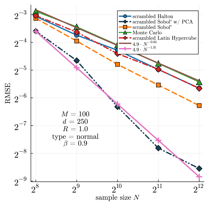
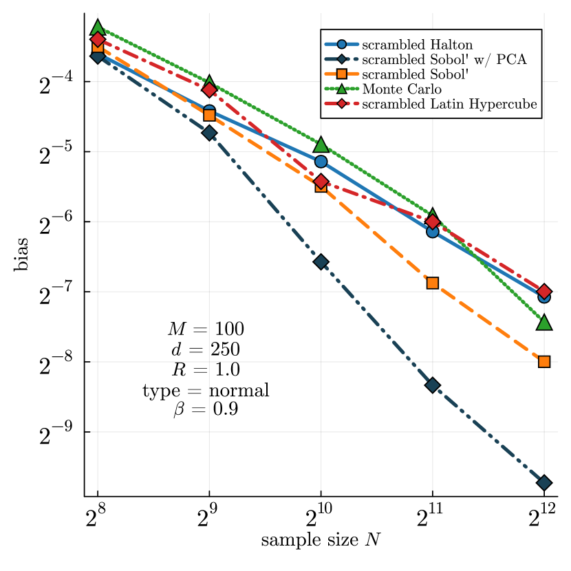
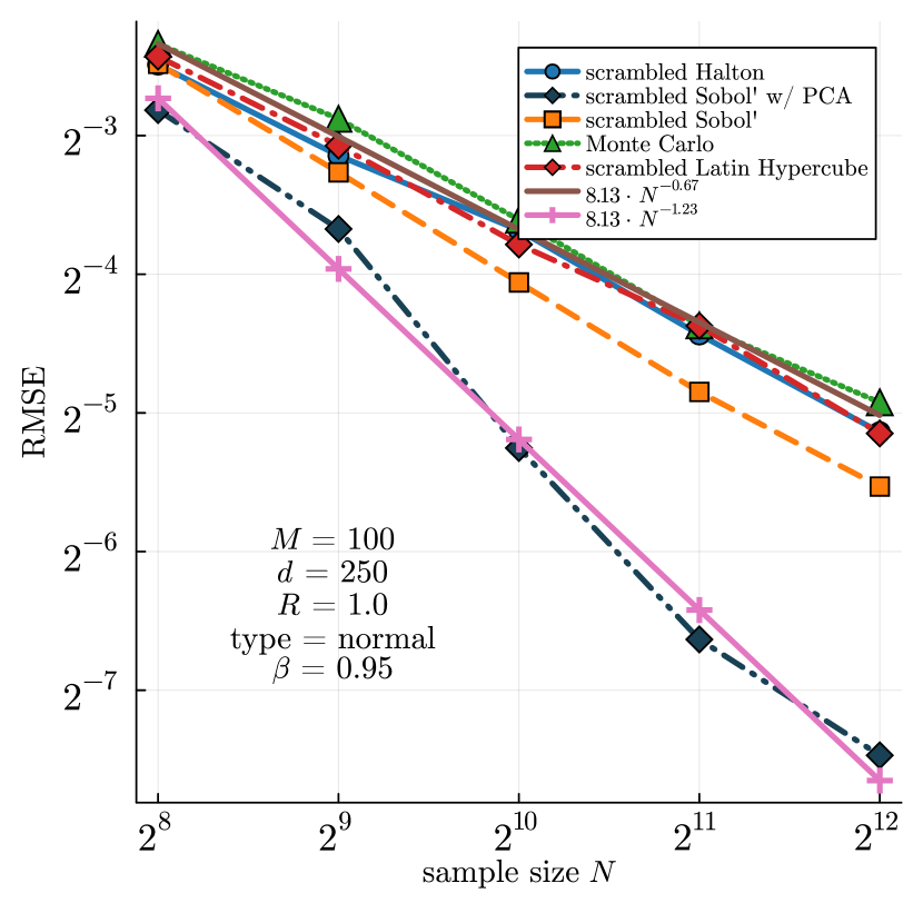
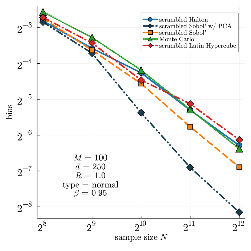
Figure 1: RMSE and bias for the sample-based approximation of Problem (21). The experiments were conducted for a normally distributed random vector $\xi$ as described in Section 6.1.1, indicated by ”type=normal.” The top two panels correspond to $\beta=0.9$, and the bottom two panels correspond to $\beta=0.95$. The value $R$ is the constraint parameter given in (21). The plots depicting the RMSE also include the least squares fit for the MC and scrambled Sobol’ experiments.

6.1.2 Linearly Transformed Uniform Samples

For our second instance, we consider a distribution of $\xi$ defined in [12, p. 471]. Specifically, we define the random vector $\xi$ by $\xi\coloneqq\mu+\sqrt{12}Q\zeta$, where $\zeta\sim\text{Uniform}[-1/2,1/2]^{d}$, and $Q$ and $\mu$ are generated as in Section 6.1.1. Unlike the case for normally distributed $\xi$, the problem does not reduce to a deterministic problem. Thus, we approximate the optimal value of (21) using its sample-based counterparts. Specifically, we solve $100$ sample-based approximations of (21) and average their optimal values. Each of these approximations is based on a realization of a scrambled Sobol’ sequence with a sufficiently large sample size. The experiment outcomes and parameter choices for Problem (21) with $\xi$ defined as in this section are shown in Figure 2.

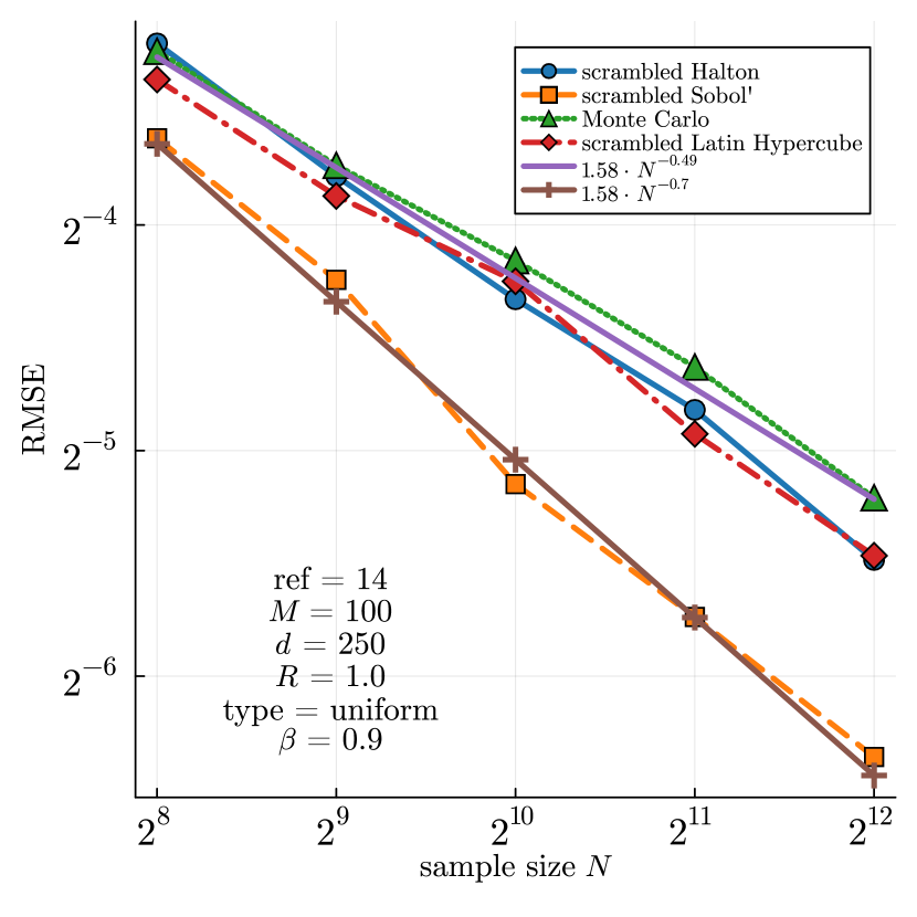
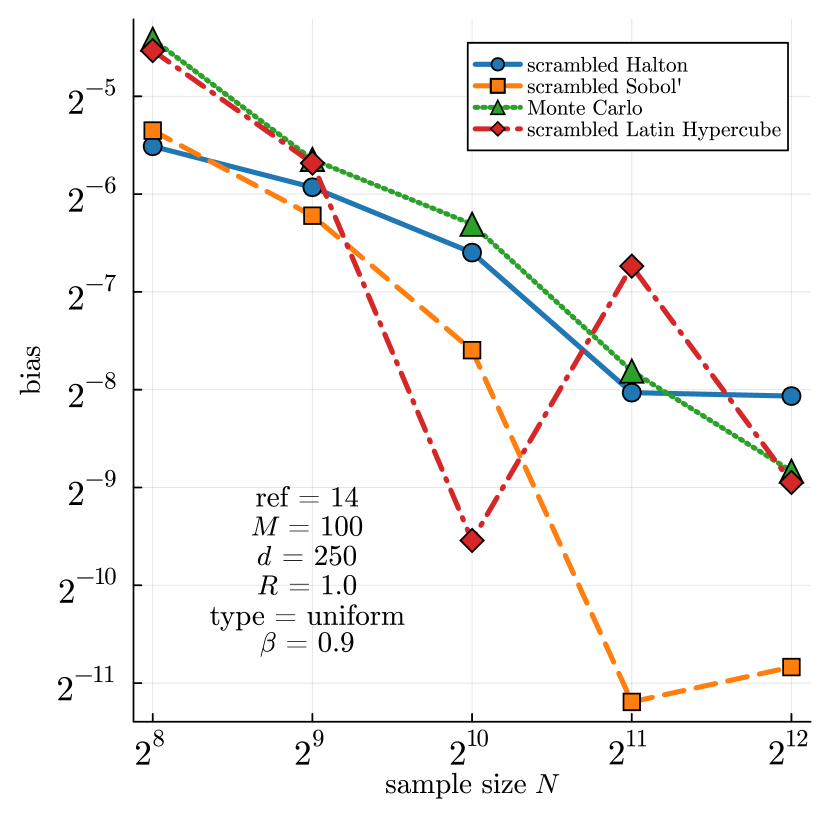
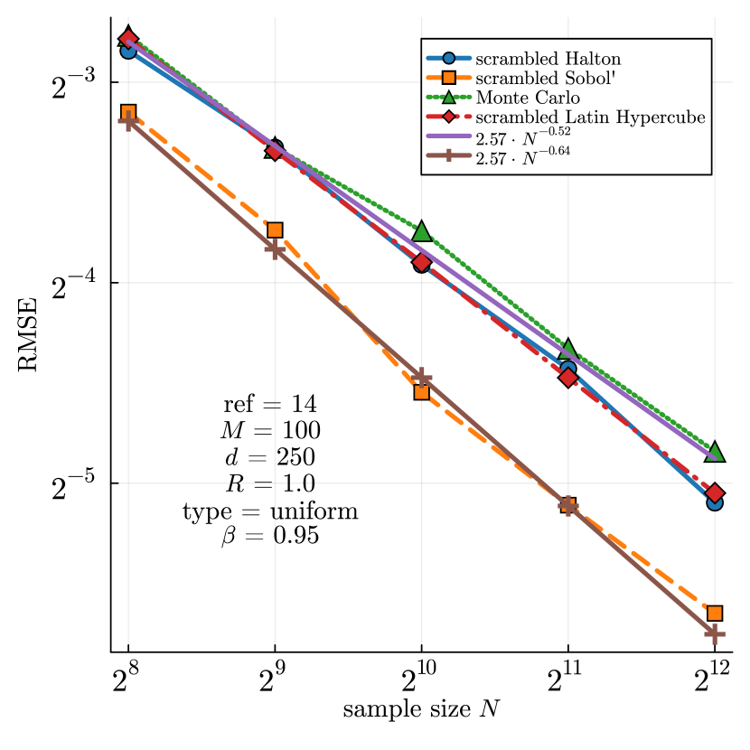
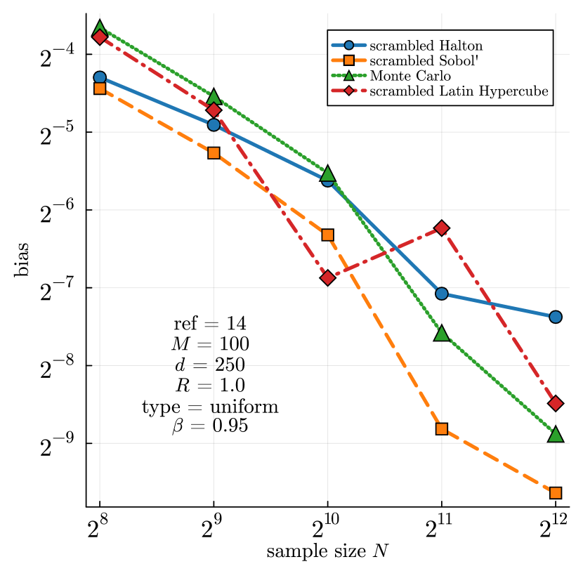
Figure 2: RMSE and bias for the sample-based approximation of Problem (21). The experiments were conducted for $\xi$ distributed as described in Section 6.1.2, indicated by ”type=uniform.” The value $R$ is the constraint parameter given in (21). The top two panels correspond to $\beta=0.9$, and the bottom two panels correspond to $\beta=0.95$. The plots depicting the RMSE also include the least squares fit for the MC and scrambled Sobol’ experiments.

6.2 A Utility Problem

The second test problem is a slight alteration of a problem in [29]. Let $(T,v,e)$ be a random vector supported on $\mathbb{R}^{md+2m}$, and let $c\in\mathbb{R}^{d}$. We consider

$$\min_{x\in\mathbb{R}^{d}}\;c^{T}x+\mathrm{CVaR}_{\beta}[Q(x,(T,v,e))] \quad\text{s.t.}\quad 0\leq x_{i}\leq 1,\quad i=1,\ldots,d,$$ (22)

where

$$Q(x,(T,v,e))\coloneqq\min_{y\in\mathbb{R}^{m}_{+}}\{y^{T}e\,\colon\quad y\geq v-Tx\}.$$

The triple $(T,v,e)$ is a reshaped and transformed random vector $\xi\sim\text{Uniform}[0,1]^{md+2m}$. In more detail, we generate samples $(T_{1},v_{1},e_{1}),(T_{2},v_{2},e_{2}),\ldots$ from random vectors $\xi^{i}\sim\text{Uniform}[0,1]^{md+2m}$ and $c$ as follows. We choose $c\sim\text{Uniform}[0,1]^{d}$. We generate the random vectors $\xi^{1},\xi^{2},\ldots,\xi^{N}\in\mathbb{R}^{md+2m}$ using (RQ)MC methods. We reshape each $\xi^{i}$ into a tuple $(T_{i},v_{i},e_{i})$ and transform the tuple such that for each $i\in\{1,\ldots,N\}$, the entries of $T_{i}$ are in $[0.5,1.0]$, those of $v_{i}$ are in $[50,100]$, and those of $e_{i}$ are in $[2,4]$. As in Section 6.1.2, we cannot solve (22) exactly. Thus, we will approximate the optimal value of (22) as in Section 6.1.2. The experiment outcomes and parameter choices for Problem (22) are depicted in Figure 3.

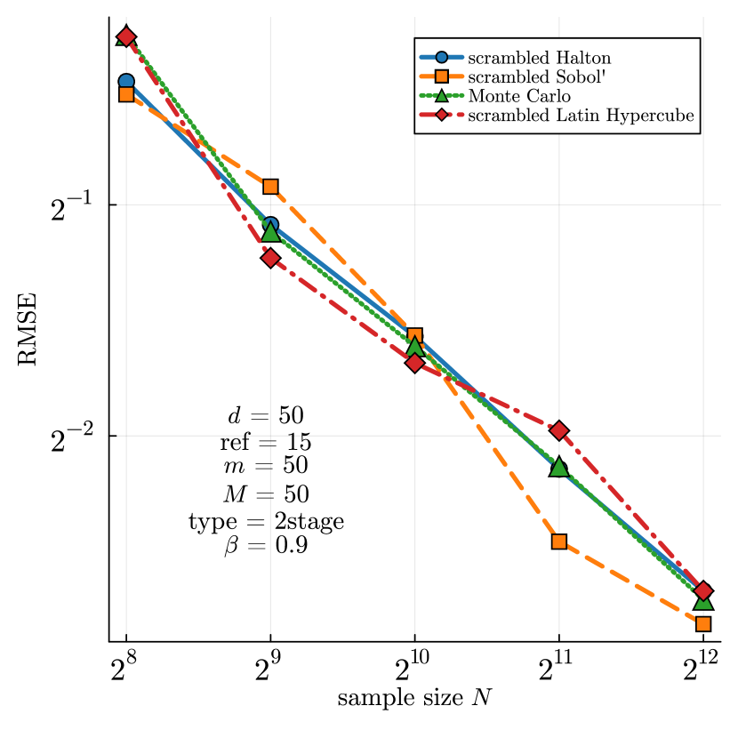
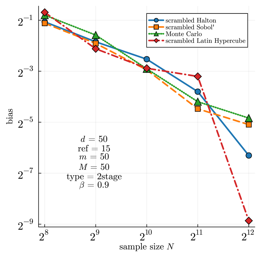
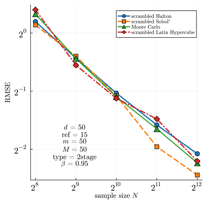
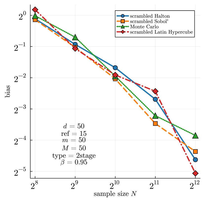
Figure 3: RMSE and bias for the sample-based approximation of Problem (22), indicated by ”type=2stage.” The top two panels correspond to $\beta=0.9$, and the bottom two panels correspond to $\beta=0.95$. The number $m$ is the dimension of $v$ and $e$ in the random element $(T,v,e)\in\mathbb{R}^{(m\times d)+m+m}$.

7 Discussion

Motivated by a SLLN for scrambled net integration [21], we have demonstrated the epiconvergence and uniform convergence for sample-based approximations of composite risk functionals, provided that the sample-based approximations satisfy a pointwise SLLN. Besides MC sampling and scrambled net integration, Latin hypercube sampling yields epiconvergent and uniform approximations.

For normally distributed random inputs, our numerical simulations show that scrambled Sobol’ integration can significantly reduce bias and RMSE when combined with dimension reduction via PCA. For the two-stage problem considered in Section 6.2, the simulation output indicates that the MC sampling and the scrambled Sobol sequences have similar RQMC and bias. In light of the theoretical considerations, discussions, and numerical simulations in [6], this could be a result of the potentially high effective dimension. Considering all of our numerical simulations and performance metrics, scrambled Sobol’ integration is always at least as good as MC sampling.

Data Availability Statement

The computer code and the simulation output is archived at https://doi.org/10.5281/zenodo.13227277.

References

- [1] H. Attouch, G. Buttazzo, and G. Michaille. Variational Analysis in Sobolev and BV spaces, volume 17 of MOS-SIAM Series on Optimization. SIAM, Philadelphia, PA, 2nd edition, 2014. doi:10.1137/1.9781611973488.
- [2] D. Bartl and L. Tangpi. Nonasymptotic convergence rates for the plug-in estimation of risk measures. Math. Oper. Res., 48(4):2129–2155, 2023. doi:10.1287/moor.2022.1333.
- [3] V. I. Bogachev. Weak convergence of measures, volume 234 of Mathematical Surveys and Monographs. American Mathematical Society, Providence, RI, 2018. doi:10.1090/surv/234.
- [4] A. Cherukuri. Sample average approximation of conditional value-at-risk based variational inequalities. Optim. Lett., 18(2):471–496, 2024. doi:10.1007/s11590-023-01996-9.
- [5] D. Dentcheva, S. Penev, and A. Ruszczyński. Statistical estimation of composite risk functionals and risk optimization problems. Ann. Inst. Statist. Math., 69(4):737–760, 2017. doi:10.1007/s10463-016-0559-8.
- [6] H. Heitsch, H. Leövey, and W. Römisch. Are quasi-Monte Carlo algorithms efficient for two-stage stochastic programs? Comput. Optim. Appl., 65(3):567–603, 2016. doi:10.1007/s10589-016-9843-z.
- [7] C. Hess. Epi-convergence of sequences of normal integrands and strong consistency of the maximum likelihood estimator. Ann. Statist., 24(3):1298–1315, 1996. doi:10.1214/aos/1032526970.
- [8] C. Hess and R. Seri. Generic consistency for approximate stochastic programming and statistical problems. SIAM J. Optim., 29(1):290–317, 2019. doi:10.1137/17M1156769.
- [9] Q. Huangfu and J. A. J. Hall. Parallelizing the dual revised simplex method. Math. Program. Comput., 10(1):119–142, 2018. doi:10.1007/s12532-017-0130-5.
- [10] A. Klenke. Probability Theory. Universitext. Springer, London, 2nd edition, 2014. doi:10.1007/978-1-4471-5361-0.
- [11] A. J. Kleywegt, A. Shapiro, and T. Homem-de Mello. The sample average approximation method for stochastic discrete optimization. SIAM J. Optim., 12(2):479–502, 2001/02. doi:10.1137/S1052623499363220.
- [12] M. Koivu. Variance reduction in sample approximations of stochastic programs. Math. Program., 103(3):463–485, 2005. doi:10.1007/s10107-004-0557-0.
- [13] G. Lan, A. Nemirovski, and A. Shapiro. Validation analysis of mirror descent stochastic approximation method. Math. Program., 134(2):425–458, 2012. doi:10.1007/s10107-011-0442-6.
- [14] W.-L. Loh. On Latin hypercube sampling. Ann. Statist., 24(5):2058–2080, 1996. doi:10.1214/aos/1069362310.
- [15] M. Lubin, O. Dowson, J. Dias Garcia, J. Huchette, B. Legat, and J. P. Vielma. JuMP 1.0: Recent improvements to a modeling language for mathematical optimization. Math. Program. Comput., 15(3):581–589, 2023. doi:10.1007/s12532-023-00239-3.
- [16] G. D. Maso. An Introduction to -Convergence, volume 8 of Progress in Nonlinear Differential Equations and Their Applications. Birkhäuser, Boston, MA, 1993. doi:10.1007/978-1-4612-0327-8.
- [17] O. Melnikov and J. Milz. Supplementary code for the manuscript: Randomized quasi-Monte Carlo methods for risk-averse stochastic optimization, August 2024. doi:10.5281/zenodo.13227277.
- [18] J. Milz and T. M. Surowiec. Asymptotic consistency for nonconvex risk-averse stochastic optimization with infinite-dimensional decision spaces. Mathematics of Operations Research, 2023. doi:10.1287/moor.2022.0200.
- [19] B. O’Donoghue. Operator splitting for a homogeneous embedding of the linear complementarity problem. SIAM J. Optim., 31(3):1999–2023, 2021. doi:10.1137/20M1366307.
- [20] A. B. Owen. Randomly permuted -nets and -sequences. In Monte Carlo and quasi-Monte Carlo methods in scientific computing (Las Vegas, NV, 1994), volume 106 of Lect. Notes Stat., pages 299–317. Springer, New York, 1995. doi:10.1007/978-1-4612-2552-2\_19.
- [21] A. B. Owen and D. Rudolf. A strong law of large numbers for scrambled net integration. SIAM Rev., 63(2):360–372, 2021. doi:10.1137/20M1320535.
- [22] T. Pennanen and M. Koivu. Epi-convergent discretizations of stochastic programs via integration quadratures. Numer. Math., 100(1):141–163, 2005. doi:10.1007/s00211-004-0571-4.
- [23] S. T. Rachev and L. Rüschendorf. Mass Transportation Problems: Vol. I: Theory. Probability and its Applications. Springer, New York, 1998. doi:10.1007/b98893.
- [24] P. T. Roy, A. B. Owen, M. Balandat, and M. Haberland. Quasi-Monte Carlo methods in Python. Journal of Open Source Software, 8(84):5309, 2023. doi:10.21105/joss.05309.
- [25] A. Shapiro. Consistency of sample estimates of risk averse stochastic programs. J. Appl. Probab., 50(2):533–541, 2013. doi:10.1239/jap/1371648959.
- [26] A. Shapiro, D. Dentcheva, and A. Ruszczyński. Lectures on Stochastic Programming: Modeling and Theory. MOS-SIAM Ser. Optim. SIAM, Philadelphia, PA, 3rd edition, 2021. doi:10.1137/1.9781611976595.
- [27] H. Sun, A. Shapiro, and X. Chen. Distributionally robust stochastic variational inequalities. Math. Program., 200(1):279–317, 2023. doi:10.1007/s10107-022-01889-2.
- [28] M. Zervos. On the epiconvergence of stochastic optimization problems. Math. Oper. Res., 24(2):495–508, 1999. doi:10.1287/moor.24.2.495.
- [29] Z. Zhang, S. Ahmed, and G. Lan. Efficient algorithms for distributionally robust stochastic optimization with discrete scenario support. SIAM J. Optim., 31(3):1690–1721, 2021. doi:10.1137/19M1290115.