Optimizing Cox Models with Stochastic Gradient Descent:
Theoretical Foundations and Practical Guidances
Abstract
Optimizing Cox regression and its neural network variants poses substantial computational challenges in large-scale studies. Stochastic gradient descent (SGD), known for its scalability in model optimization, has recently been adapted to optimize Cox models. Unlike its conventional application, which typically targets a sum of independent individual loss, SGD for Cox models updates parameters based on the partial likelihood of a subset of data. Despite its empirical success, the theoretical foundation for optimizing Cox partial likelihood with SGD is largely underexplored. In this work, we demonstrate that the SGD estimator targets an objective function that is batch-size-dependent. We establish that the SGD estimator for the Cox neural network (Cox-NN) is consistent and achieves the optimal minimax convergence rate up to a polylogarithmic factor. For Cox regression, we further prove the -consistency and asymptotic normality of the SGD estimator, with variance depending on the batch size.
Furthermore, we quantify the impact of batch size on Cox-NN training and its effect on the SGD estimator’s asymptotic efficiency in Cox regression. These findings are validated by extensive numerical experiments and provide guidance for selecting batch sizes in SGD applications. Finally, we demonstrate the effectiveness of SGD in a real-world application where GD is unfeasible due to the large scale of data.
keywords:
Cox model; linear scaling rule; minimax rate of convergence; neural network; stochastic gradient descent.1 Introduction
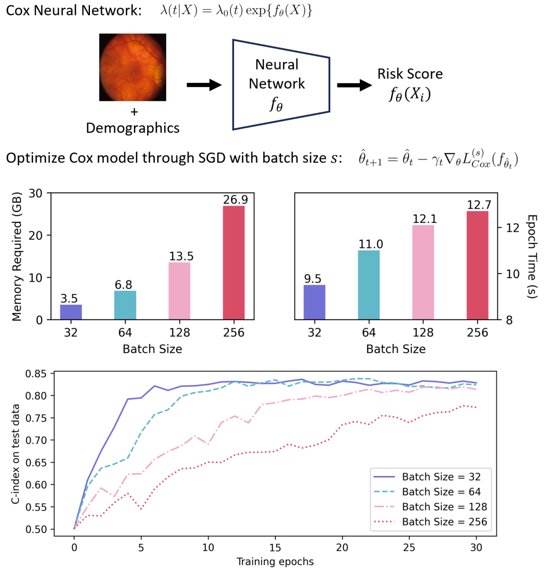
Cox proportional-hazard regression (Cox 1972) is one of the most commonly used approaches in survival analysis, where the primary outcome of interest is the time to a certain event. It assumes that the covariates have a linear effect on the log-hazard function. With the development of deep learning, Cox proportional-hazard-based neural networks (Cox-NN) have been proposed to model the potential nonlinear relationship between covariates and survival outcomes and improve survival prediction accuracy (Faraggi and Simon 1995; Katzman et al. 2018; Ching et al. 2018; Zhong et al. 2022). Despite the success of Cox models in survival analysis, they face a significant optimization challenge when applied to large-scale survival data. In particular, the Cox models are typically trained by maximizing the partial likelihood (Cox 1975) through the gradient descent (GD) algorithm, which requires the entire dataset to compute the gradient. This can be slow and computationally extensive for large datasets. For example, as shown in Figure 1, performing GD in Cox-NN training requires more than 500 GB of memory, which makes GD impractical due to hardware memory limitations. Besides Cox-NN, the large-scale data also challenges the optimization of Cox regression. Tarkhan and Simon (2024) reported that the GD algorithm for Cox regression is vulnerable to round-off errors when dealing with large sample sizes. Consequently, GD optimization constrains Cox models’ scalability in large-scale data applications.
Stochastic gradient descent algorithm (SGD) is a scalable solution for optimization in applications with large-scale data and has been widely used for NN training (Amari 1993; Hinton et al. 2012; Bottou 2012). It avoids the calculation and memory burdens by using a randomly selected subset of the dataset, which is called a mini-batch, to calculate the gradient and update parameters in each recursion. In NN optimization, SGD also accelerates the convergence process, as the inherent noise from the stochastic nature of mini-batches helps escape from the local minimizer (Kleinberg et al. 2018). Unfortunately, SGD cannot be directly used to optimize the partial likelihood of all samples because calculating the individual partial likelihood requires access to all data that survived longer (at risk). This makes it unclear how to optimize the Cox model through SGD.
Several attempts have been made to enable parameter updates of the Cox model using the mini-batch data. Kvamme et al. (2019) followed the idea of nested case-control Cox regression from Goldstein and Langholz (1992), proposing an approximation of the gradient of partial likelihood from the case-control pairs instead of using all at-risk samples. This strategy worked well in practice, making it possible to fit the Cox model with SGD. Sun et al. (2020) fitted a Cox-NN to establish a prediction for eye disease progression through SGD where the recursion was based on the partial likelihood of a subset of data. Recently, Tarkhan and Simon (2024) studied the SGD for Cox regression in online learning and demonstrated that the maximizer of the expected partial likelihood of any subset is the true parameter under the Cox regression model. This observation and the practical successes imply that the Cox models can be optimized through the SGD, but lack the theoretical guarantee.
Motivated by the knowledge gap, in this work, we establish theoretical foundations for employing SGD in Cox models, where the gradient is calculated only on a subset of data and is, therefore, scalable for large-scale applications. Specifically, our contributions come from the following three folds:
-
•
Firstly, the SGD estimator of the Cox models does not optimize the partial likelihood of all samples (Cox 1975) but optimizes a different function. Therefore, it is unclear whether the SGD estimator is valid. We establish the asymptotic properties of the SGD estimators for Cox models. For Cox-NN, we show that the SGD estimator is consistent with the unknown true function and able to circumvent the curse of dimensionality. It achieves the minimax optimal convergence rate up to a polylogarithmic factor. For Cox regression, we prove the SGD estimator is -consistent, asymptotically normal. These results justify the application of SGD algorithm in the Cox model.
-
•
Secondly, the target function optimized by SGD for the Cox model is batch-size dependent. We present the properties of this function and demonstrate how its curvature changes with the batch size. We further investigate the impact of batch size in Cox-NN training and provide both theoretical and numerical evidence that (the ratio of the learning rate to the batch size) is a key determinant of SGD dynamics in Cox-NN training. Keeping the ratio constant makes the Cox-NN training process almost unchanged (linear scaling rule). Additionally, for Cox regression, we demonstrate the improvement in statistical efficiency when batch size doubles. This phenomenon is not seen in SGD optimizations such as minimizing the mean squared error where the estimators’ statistical efficiency is independent of the SGD batch size.
-
•
Lastly, we study the convergence of the SGD algorithm in terms of iteration for Cox regression. We note that the target loss function optimized by SGD is not strongly convex and an additional projection step is needed in the SGD recursion (projected SGD). We perform the non-asymptotic analysis of the projected SGD algorithm and demonstrate the algorithm converges to the global minimizer with large enough iterations.
The rest of the paper is organized as follows. We introduce the Cox models and SGD with necessary notations in Section 2. We establish the theoretical properties of SGD estimators for Cox-NN and investigate the impact of batch size in Cox-NN training in Section 3. The theoretical properties of SGD estimators for Cox regression as well as the convergence of SGD algorithm over iterations are studied in Section 4. Section 5 presents simulation studies and a real-world data example.
2 Background and Problem Setup
Let denote observed independent and identical distributed (i.i.d.) samples. Survival analysis is to understand the effect of covariate on the time-to-event variable (e.g., time-to-death). Let denote the true censoring time. Due to the right censoring, the observed time-to-event data is the triplet set , where is the observed time and is the event indicator.
2.1 Cox Model and Deep Neural Network
Cox model assumes that the hazard function takes the form
| (2.1) |
where is an unspecified baseline hazard function. The covariate influences the hazard through the unknown relative risk function . When , the model (2.1) is the Cox regression model where the effect of is linear. When the form is unspecified and is approximated through a neural network with parameter , we refer to it as Cox-NN. We briefly review the NN structure:
Let be a positive integer and be a positive integer sequence. A -layer NN with layer-width , i.e. number of neurons, is a composite function recursively defined as
| (2.2) |
where the matrices and vectors (for ) are the parameters of the NN. The pre-specified activation function is a nonlinear transformation that operates componentwise on a vector, that is, , which thus gives for . Among the activation functions that have been widely considered in deep learning, we focus on the most popular one named Rectified Linear Units (ReLU) in Nair and Hinton (2010) throughout this paper:
which is also considered in Schmidt-Hieber (2020) and Zhong et al. (2022). For NN in (2.2), denotes the depth of the network. The vector lists the width of each layer with the first element as the dimension of the input variable, are the dimensions of the hidden layers, and is the dimension of the output layer. The matrix entries are the weight linking the th neuron in layer to the th neuron in layer , and the vector entries represent a shift term associated with the th neuron in layer . In Cox-NN, the output dimension as the output of the is a real value.
The standard optimization of the Cox model is through minimizing the negative log-partial likelihood function defined as
| (2.3) |
where sample who has experienced the event () is compared against all samples that have not yet experienced the event up to time (i.e., “at risk” set). The minimizer of (2.3) is typically found using gradient-descent-based algorithms where the gradient is calculated using samples in each iteration (Therneau et al. 2015; Katzman et al. 2018; Zhong et al. 2022). The statistical properties of the minimizer have been well-studied by Cox (1972); Andersen and Gill (1982) for Cox regression and by Zhong et al. (2022) for Cox-NN.
Note that all the above studies optimize the Cox model through GD. However, when optimizing the Cox model through the SGD algorithm using a subset of samples, it does not minimize (2.3), which will be further explained in the next section.
2.2 Stochastic Gradient Descent for Cox Model
We start this section with a brief review of the general SGD algorithm. In the SGD iterations, the gradient is estimated on a subset of data . The subset is called a mini-batch with batch size . Throughout this paper, we consider the batch size is fixed and does not depend on the sample size . Let be an empirical loss function of samples. To find the minimizer of , at the th iteration step of SGD, the parameter is updated through
| (2.4) |
where is a pre-scheduled learning rate for the th iteration. is the gradient calculated from the mini-batch data at th iterations. To ensure converges to over the iterations, SGD requires that
| (2.5) |
for all , where the expectation is over the randomness of generating from . The equality (2.5) indicates that the gradient based on should be an unbiased estimator of at any given . Throughout the paper, we consider is randomly sampled from at each iteration, therefore the distribution does not depend on . To simplify the notation, for any , we omit the input data and drop the subscript and let , , if no confusion arises.
The requirement (2.5) is satisfied in the SGD optimizations for the mean squared error, where the gradient function is the average of individual gradient, that is . Let and is generated by randomly sampling subjects without replacement from , we have
| (2.6) |
For Cox models, the SGD implementation (Kvamme et al. 2019; Tarkhan and Simon 2024) requires at least two samples to calculate the gradient, which restricts . The parameters are updated through
| (2.7) |
where the gradient from is calculated by
| (2.8) |
and the at-risk set is constructed on . Note that (2.8) can not be written as the average of i.i.d. gradients. Follow the requirement (2.5), and suppose is generated by randomly sampling subjects without replacement from , the SGD recursion (2.7) is to solve the root of
| (2.9) |
Note that the right side of (2.9) is different from in Cox model, which indicates the target function solved by SGD differs from the one solved by GD. Therefore, the theoretical results for the GD estimator can not be applied to the SGD estimator. This motivates us to investigate the statistical properties of the root of , or equivalently the minimizer of .
We make the following standard assumptions for the time-to-event data with right-censoring:
-
(A1)
The true failure time and true right-censoring time are independent given the covariates .
-
(A2)
The study ends at time and there exists a small constant such that and almost surely with respect to the probability measure of .
-
(A3)
takes value in a bounded subset of with probability function bounded away from zero. Without loss of generality, we assume that the domain of is taken to be .
Assumptions (A1)-(A3) are common regularity assumptions in survival analysis.
3 SGD Estimator for Cox Neural Network
Zhong et al. (2022) studied the asymptotic properties of the NN estimator which minimizes (2.3) by GD. They showed that the NN estimator achieves the minimax optimal convergence rate up to a polylogarithmic factor. Our work is inspired by the theoretical developments in Zhong et al. (2022) but has major differences. First, Zhong et al. (2022) shows the at-risk term converges to a fixed function . However, in SGD with a fixed , the at-risk term in always consists of samples. Thus both the empirical loss and the population loss are different from Zhong et al. (2022) and depend on . Second, when is generated by randomly sampling subjects without replacement from in each iteration, is an average over combinations of the mini-batch, where different batches may share the same samples. Hence the correlation between the batches needs to be handled when deriving the asymptotic properties of the minimizer of .
3.1 Consistency and Convergence Rate of SGD Estimator
Following Schmidt-Hieber (2020) and Zhong et al. (2022), we consider a class of NN with sparsity constraints defined as
| (3.1) |
where and denotes the sup-norm of matrix or vector, is the number of nonzero entries of matrix or vector, and is the sup-norm of the function . and the sparsity is a positive integer. The sparsity assumption is employed due to the widespread application of techniques such as weight pruning (Srinivas et al. 2017) or dropout (Srivastava et al. 2014). These methods effectively reduce the total number of nonzero parameters, preventing neural networks from overfitting, which results in sparsely connected NN. We approximate in (2.1) using a NN parameterized by . More precisely, is estimated by minimizing through SGD procedure (2.7) and is generated by randomly sampling subjects without replacement from . To simplify the notation, we omit and denote the estimator by
| (3.2) |
where . We use the superscript to indicate its dependency on the batch size .
Some restrictions on the unknown function are needed to study the asymptotic properties of . We assume belongs to a composite smoothness function class, which is broad and also adopted by Schmidt-Hieber (2020) and Zhong et al. (2022). Specifically, let be a Hø̈lder class of smooth functions with parameters and domain defined by
where is the largest integer strictly smaller than , with , and .
Let , and , with , where is the set of all positive real numbers. The composite smoothness function class is
| (3.3) |
where is the intrinsic dimension of the function. For example, if
and are twice continuously differentiable, then smoothness , dimensions and . We assume that
-
(N1)
The unknown function is an element of
The mean zero constraint in (N1) is for the identifiability of since the presence of two unknown functions in (2.1).
We denote and with notation . Furthermore, we denote as for some and any . means and . We assume the following structure of the NN:
-
(N2)
, and .
A large neural network leads to a smaller approximation error and a larger estimation error. Assumption (N2) determines the structure of the NN family in (3.1) and has been adopted in Zhong et al. (2022) as a trade-off between the approximation error and the estimation error.
We first present a lemma which is critical to study the asymptotic properties of :
Lemma 3.1
Let . Under the Cox model, with assumption (A1)-(A3), (N1) and for any integer and constant , we have
for all , where .
Remark 3.2
Suppose and by definition . On the other hand, we have from Lemma 3.1. Hence, and it implies . That is for any integer , the minimizer of on a neighborhood of is and does not depend on . It is a generalization of the result in Tarkhan and Simon (2024) where they consider a parametric function with the truth and demonstrate that for any integer .
Then we obtain the result regarding the asymptotic properties of the SGD estimator for Cox-NN:
Theorem 3.3
Under the Cox model, with assumptions (A1)-(A3), (N1), (N2) and for any integer , there exists an estimator in (3.2) satisfying , such that
Remark 3.4
Remark 3.5
Theorem 3.3 demonstrates that the convergence rate is determined by the smoothness and the intrinsic dimension of the function , rather than the dimension . Therefore, the estimator can circumvent the curse of dimensionality (Bauer and Kohler 2019). It has a fast convergence rate when the intrinsic dimension is relatively low.
Remark 3.6
The minimax lower bound for estimating can be derived following the proof of Theorem 3.2 in Zhong et al. (2022) as their Lemma 4 and derivations still hold without the parametric linear term. Specifically, let . Under the Cox model with assumptions (A1)-(A3) and (N1), there exists a constant , such that , where the infimum is taken over all possible estimators based on the observed data. Therefore, the NN-estimator in Theorem 3.3 is rate optimal since it attains the minimax lower bound up to a polylogarithm factor.
Remark 3.7
Note that the smallest batch size that can be chosen is and is nonzero only when one subject experiences the event while another remains at risk at that time. Kvamme et al. (2019) proposes first sampling subjects experiencing the event and then sampling one subject from the corresponding at-risk set for each event in each SGD iteration, thus forming case-control pairs. They observed that utilizing the average gradient of over the pairs in SGD updates results in an effective estimator for . This can be attributed to the fact that is a valid loss function for , as demonstrated in Lemma 3.1 and Theorem 3.3.
3.2 Impact of Mini-batch Size on Cox-NN Optimization
Section 3.1 presents the statistical properties of the global minimizer . Whether can be reached by SGD is affacted by many factors since the NN training is a highly non-convex optimization problem (see the visualization by Li et al. (2018)). When applying SGD in NN training, the learning rate and batch size and greatly influence the behavior of SGD. It has been noticed that the ratio of the learning rate to the batch size is a key determinant of the SGD dynamics (Goyal et al. 2017; Jastrzebski et al. 2017, 2018; Xie et al. 2020). A lower value of leads to a smaller size of the step. Goyal et al. (2017) demonstrates a phenomenon that keeping constant makes the SGD training process almost unchanged on a broad range of minibatch sizes, which is known as the linear scaling rule. This rule guides the tuning of hyper-parameters in NN such that we can fix either or and only tune the other parameter to optimize the behavior of SGD.
Whether the linear scaling rule can be applied to Cox-NN training is questionable since the population loss in Cox-NN depends on the batch size. Previous theoretical works focused on the population loss whose convexity is invariant to different batch sizes and assumed that the Hessian equals the covariance of gradient at the truth, that is (Jastrzebski et al. 2017, 2018; Xie et al. 2020). For example, the population loss for MSE satisfies both assumptions and hence the linear scaling rule holds in this case. However, these key assumptions are violated as shown in the following theorem for the population loss under the Cox model.
Theorem 3.8
Under the Cox model with parameterized by , with assumption (A1)-(A3) and suppose , exist and ,, are bounded for all on a neighborhood of , then for any integer we have
| (3.4) |
and
| (3.5) |
where is second-order derivative operator with respect to and denotes is semi-positive definite.
Remark 3.9
With Theorem 3.8, we demonstrate the linear scaling rule in Cox-NN training still holds, especially when the batch size is large. Following the derivation in Section 2.2 of Jastrzebski et al. (2017), is the key determinant of the dynamics of SGD in Cox-NN, where and Tr() is the trace. When doubles, the difference of Hessian trace is at most and negligible for large (see Supplementary Materials for more discussion). Therefore, the linear scaling rule still holds for Cox-NN when batch size is large. In Section 5, we numerically demonstrate that the increase of is small for and the linear scaling rule holds in Cox-NN training for large batch size.
4 SGD Estimator for Cox Regression
In this section, we consider the Cox regression model with where the effect of is linear and estimate through the SGD procedure (2.7) with
| (4.1) |
We adopt the following assumptions for the regression setting:
-
(R1)
The true relative risk with parameter .
-
(R2)
There exist constants such that the subdensities of satisfies for all .
-
(R3)
For some and , the th partial derivative of the subdensity of with respect to exists and is bounded.
The subdensity is defined as
Assumption (R2) ensures the information bound for exists. Assumption (R3) is used to establish the asymptotic normality of the SGD estimator. Moreover, assumption (R1) and (R2) are necessary to demonstrate the strong convexity of , i.e., for all .
Depending on the nature of the dataset, we study the SGD estimator for Cox regression under the offline scenario (unstreaming data) and the online scenario (streaming data). In the first scenario, the dataset of i.i.d. samples has been collected. In the second scenario, the observations arrive in a continual stream of strata, and the model is continuously updated as new data arrives without storing the entire dataset.
4.1 SGD for Offline Cox Regression
To study the statistical properties of , we consider two sampling strategy of which determines the form of . The first strategy has been considered in Theorem 3.3 where is generated by randomly sampling subjects from without replacement. We refer to it as stochastic batch (SB) with the estimator
| (4.2) |
Another strategy is to randomly split the whole samples into non-overlapping batches. Once the mini-batches are established, they are fixed and then repeatedly used throughout the rest of the algorithm (Qi et al. 2023). We refer to it as fixed batch (FB) with the estimator
| (4.3) |
where we use to denote that has been partitioned into fixed disjoint batches. The element of is a mini-batch containing i.i.d. samples and is generated by randomly picking one element from . We consider the second sampling strategy because it is a popular choice in the SGD application and the impact of batch size on the asymptotic variance of can be well-established.
We present the asymptotic properties of and in the following theorem:
Theorem 4.1
Under the Cox model, with assumptions (A1)-(A3), (R1)-(R3) and for any integer , we have
| (4.4) | ||||
| (4.5) |
when , where , , and
which is the covariance of on two mini-batches sharing the same sample but different rest samples (denoted by ).
Remark 4.2
Theorem 4.1 states that, for any choice of batch size , both and converge to at speed. Additionally, they are asymptotically normal with a sandwich-type variance while the middle part of the asymptotic variance differs. By the theory of the U-statistics (Hoeffding 1992), we have and the equality holds only if can be written as the average of i.i.d. gradients, such as the mean squared error in (2.6). Because this condition does not hold for presented in (2.8), it implies that and therefore is asymptotically more efficient than . This is not typically observed in SGD optimizations. Take (2.6) for instance, one can verify that and is therefore as efficient as for mean squared error.
Remark 4.3
The convergence rate established in Theorem 3.3 still holds if we consider the FB strategy for NN training and replace the empirical loss in (3.2) by . The proof is even simpler because there are no correlations between the batches and the empirical loss is the average of i.i.d. tuples. Hence, the convergence rate is , which is equivalent to as with being a fixed constant.
The impact of batch size on the asymptotic variances can be explicitly described by the following Corollary from Theorem 3.8:
Corollary 4.4
Under the Cox model, suppose the assumptions in Theorem 4.1 holds, then for any integer , we have
| (4.6) |
and
| (4.7) |
Remark 4.5
Equality (4.6) indicates that the asymptotic variance of is . Then by (4.7), we have , i.e., the asymptotic efficiency of improves when the doubles. The asymptotic variance of can not be further simplified to directly evaluate the impact of batch size. Nevertheless, the decrease of its upper bound implies the efficiency improvement when batch size doubles. Moreover, such an impact of batch size on the asymptotic variance is not typically observed in SGD optimizations. Take the minimization of mean square error in (2.6) for instance, one can verify that degenerates to which is not depending on .
Remark 4.6
To the best of our awareness, the equivalence of and has not been studied. Theorem 4.1 shows that these two quantities determine the asymptotic variance of SGD estimators in Cox regression. Moreover, one can verify that
when where is the information matrix of . This demonstrates that decreases towards its lower bound as continues doubling, suggesting that the SGD estimator is less efficient than the GD estimator, whose asymptotic variance is . Moreover, when batch size is large and is approaching , the efficiency gain from doubling the batch size would diminish, which has been empirically reported in Goldstein and Langholz (1992); Tarkhan and Simon (2024).
4.2 SGD for Online Cox Regression
In contrast to the offline Cox regression where the target is to minimize the empirical loss , the online Cox regression minimizes the population loss by directly sampling the mini-batch from the population. For online learning, it is of interest to study the convergence of to as well as its asymptotic behavior when the iteration step , where is the estimator at th recursion in (2.4). Note that this is an optimization problem of whether an algorithm can reach the global minimizer over the iterations. It differs from our previous investigation of an estimator’s asymptotic properties with large sample size, where the estimator is the global minimizer of empirical loss.
Strong convexity of the target function is critical to establish the convergence of SGD algorithm to the global minimizer (Ruppert 1988; Polyak and Juditsky 1992; Toulis and Airoldi 2017). It requires the function to grow as fast as a quadratic function. Specifically, function is strongly convex if and only if there exists a constant and for all where is an identity matrix. Unfortunately, the population loss of online Cox regression
is not strongly convex over . It can be easily verified when and when . Nonetheless, we notice that is strongly convex on any compact set covering the true parameter :
Lemma 4.7
Suppose the integer and . Then under Cox model, with assumptions (A1)-(A3), (R1), (R2), there exist a constant such that for any
The radius can be arbitrarily large so that covers the true parameter to guarantee is strongly convex on . Therefore, a modification of (2.7) could be applied to restrict the domain of and establish the convergence of SGD algorithm for Cox regression, which is called projected SGD. That is,
| (4.8) |
where is the orthogonal projection operator on the ball (Moulines and Bach 2011). The projection step ensures the iterations are restricted to the area where is strongly convex. Then we have the following non-asymptotic result for the projected SGD algorithm by confirming the conditions of Theorem 2 in Moulines and Bach (2011):
Theorem 4.8
Remark 4.9
This result demonstrates the convergence of projected SGD to the global minimizer of with large enough iterations. When , the convergence is at rate . When , we have if , if , and if . Therefore, when , the choice of is critical. If is too small, the convergence is at an arbitrarily small rate . While a large leads to the optimal convergence rate , the term would be large and result in an increasing bound when is small so that the orthogonal projection should be repeatedly operated in the early phase of the training, which leads to additional calculation cost. The optimal convergence rate can be achieved regardless of by averaging. Lacoste-Julien et al. (2012) showed that, for projected SGD recursion (4.8) and if the target loss is strongly convex on , then with learning rate for any , where .
Remark 4.10
The convergence of SGD for offline Cox regression can be similarly established. If is sampled from the using either method considered in Section 4.1, and if is finite, then will converge to over the iterations (2.7). This justifies our previous investigation of the statistical properties of , as it can be reached by SGD algorithm. The sufficient condition on a given for the finiteness of can be derived following Chen et al. (2009). Please refer to the Supplementary Materials for more details.
5 Numerical Implementation and Results
5.1 Impact of Batch Size on the Convexity
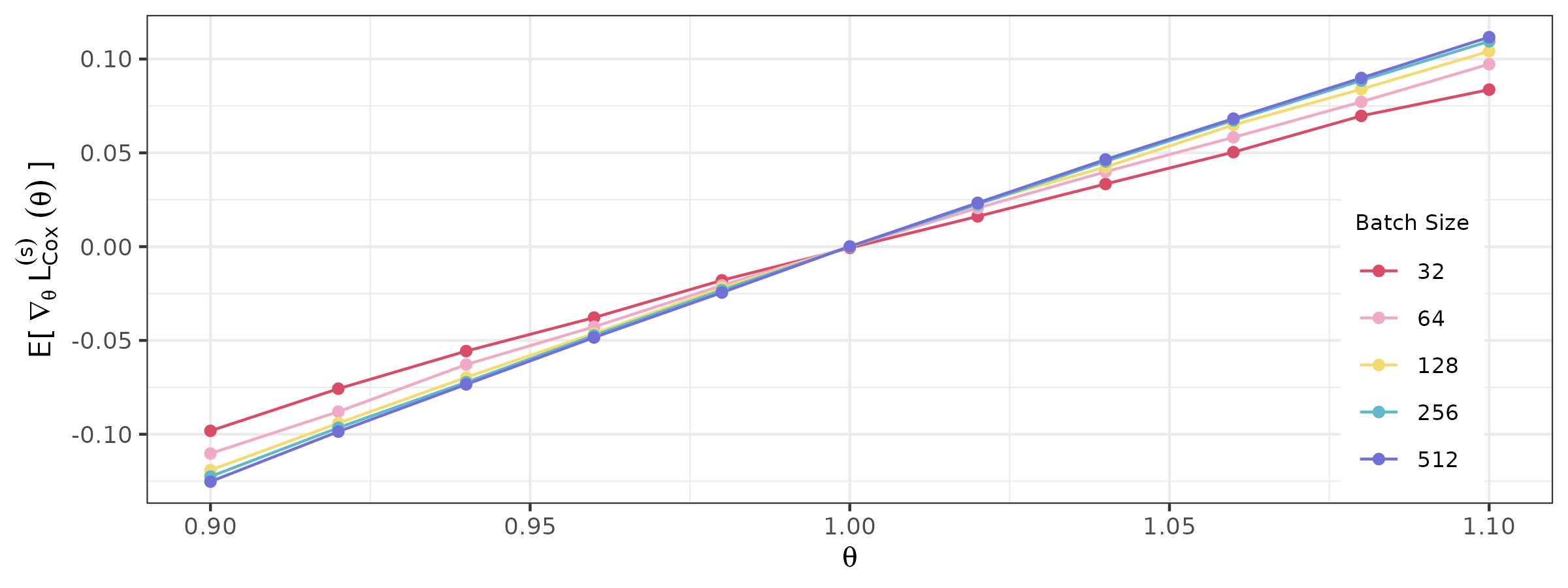
We performed numerical experiments to evaluate the relation between and in Cox-regression with . We set and follows a uniform distribution . For each , we estimated on a neighborhood of from the average of 20,000 realizations of , where each realization consists of i.i.d. time-to-event data from a Cox model with and an independent censoring distribution.
Figure (2(a)) presents at a neighborhood of with different batch size . It verifies as we observe the slope increment of at the truth when batch size doubles. The increment is negligible for a large as discussed in Remark 4.6. Moreover, is always the root of regardless the choice of .
5.2 Linear Scaling Rule for Cox Neural Network
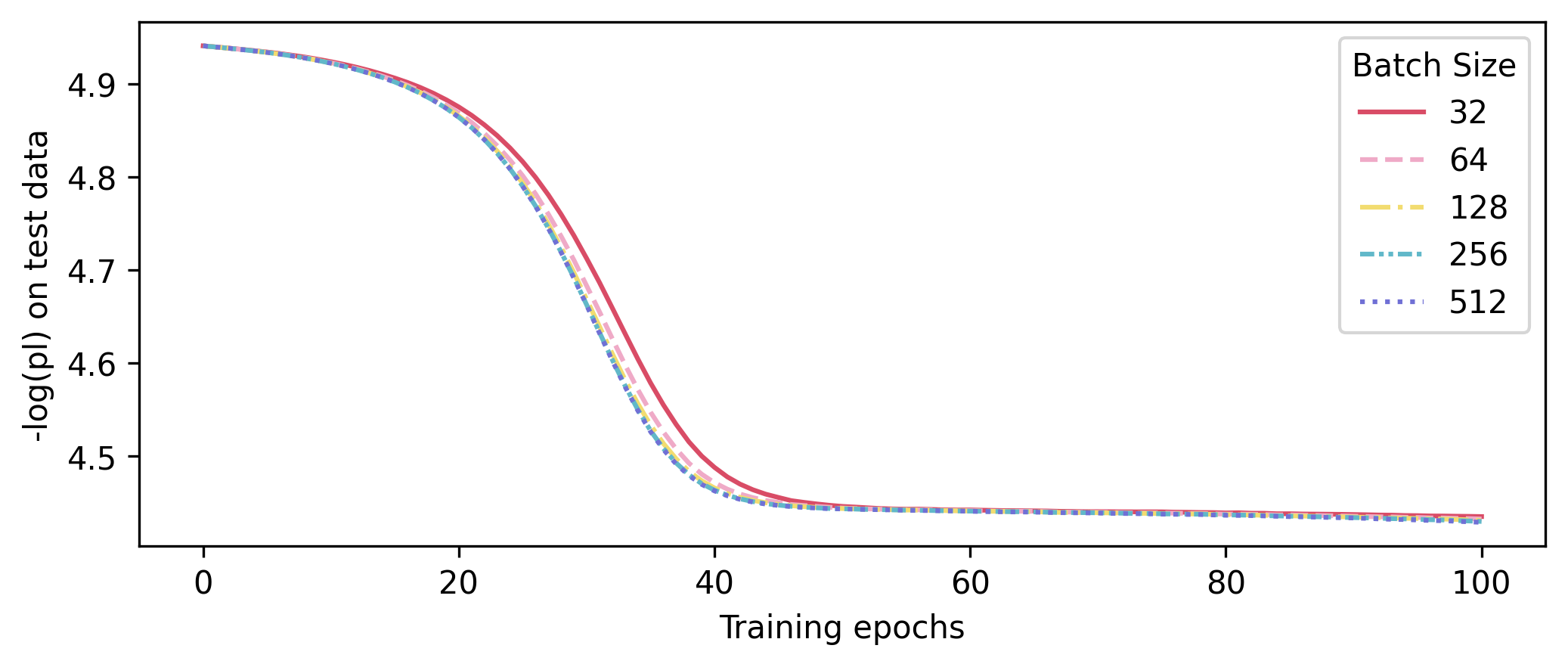
We conducted a numerical experiment to evaluate whether keeping (learning rate/ batch size) constant makes the SGD training process unchanged in Cox-NN. The true event time is generated from a distribution with true hazard function where and
where is to center towards zero. The observed data is where is generated from an independent exponential distribution. We adjust the parameter of the exponential distribution to make the censoring rate . Cox-NN is fitted on the survival data and the full negative log-partial likelihood is calculated on the test data to make a fair comparison when choosing different batch sizes. Identical to the spirit of Goyal et al. (2017), our goal is to match the test errors across minibatch sizes by only adjusting the learning rate, even better results for any particular minibatch size could be obtained by optimizing hyper-parameters for that case. Figure (2) shows that the linear scaling rule still holds in Cox-NN while the slight differences between the training trajectories are due to the convexity change of the loss function with different choice of batch size.
5.3 Impact of Batch-size in Cox Regression
We carried out the simulations to empirically assess the impact of batch size in Cox regression. The survival data generating mechanism is identical to Section 5.2 except for the true event time is from where , and Uniform(0,1) for . We performed projected SGD (4.8) with and initial point to estimate based on samples. The SGD batch size is set as where . The total number of epochs (training the model with all the training data for one cycle) is fixed as and the learning rate is set as which decreases after each epoch. Besides SGD-SB and SGD-FB, we also fit a stratified Cox model (CoxPH-strata) by treating the fixed batches from FB strategy as strata. Note that CoxPH-strata directly solves Eq. (4.3) and gives from GD algorithm. The convergence of SGD to can be evaluated by comparing the estimators from SGD-FB and CoxPH-strata. CoxPH is fitted under the standard function using all samples. The simulation is repeated for 200 runs.
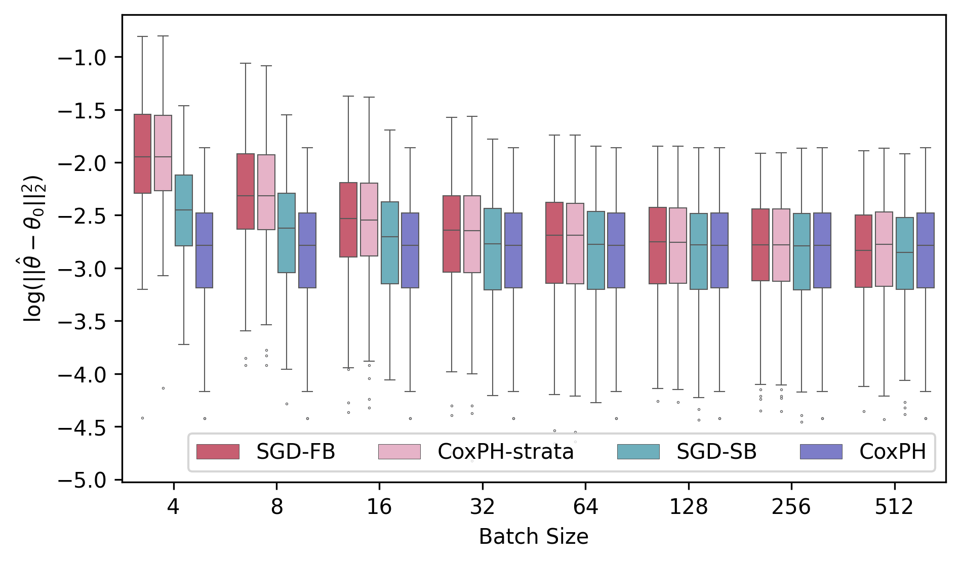
We note that stays inside of throughout the iterations. Hence the projection step is redundant in the simulation and (4.8) degenerates to (2.7). Simulation results are presented in Figure 3. The convergence of SGD is validated by confirming the loss curve’s stability over epochs as well as the small difference between the SGD estimator and the estimator from CoxPH-strata . Actually for all throughout the simulations. As expected, SGD-SB is more efficient than SGD-FB. For both SGD-SB and SGD-FB, there is efficiency loss when batch size is small. The efficiency loss is negligible when the batch size is larger than 128 in our simulation.
5.4 Real Data Analysis
We applied the Cox-NN on Age-Related Eye Disease Study (AREDS) data and built a prediction model for time-to-progress to the late stage of AMD (late-AMD) using the fundus images. The analysis data set includes 7,865 eyes of 4,335 subjects with their follow-up time and the disease status at the end of their follow-up. Our predictors include three demographic variables (age at enrollment, educational level, and smoking status) and the fundus image. The size of the raw fundus image is . We cropped out the middle part of fundus image and resized it to . In this application, the Cox-NN employs ResNet50 structure (He et al. 2016) to take fundus image as input. Cox-NN is optimized through SGD on a training set (7,087 samples) using Nvidia L40s GPU with 48 GB memory and then evaluated in a separate test set (778 samples). In Figure 1, we list the memory required to perform SGD and epoch time with different choices of batch size in SGD. The size of 7,087 fundus images in training data is 3.97 GB. Besides loading the batch data, additional memories are needed to store the model parameters and the intermediate values for the gradient computation. Therefore, less memory is required to perform SGD with a smaller batch size. The GD is equivalent to set batch size as 7,087 and can not be performed in this application. In addition to the lower memory requirement, the time to process the training data for one cycle (one epoch) is shorter for the SGD with a smaller batch size.
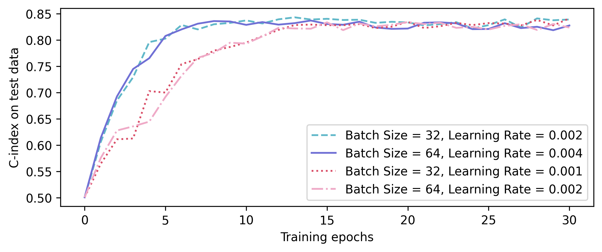
From the trajectories of C-index over the training epochs in Figure 4, it justifies our discussion in Section 3.2 that the ratio of learning rate to batch size determines the dynamics of SGD in Cox-NN training. The SGD training history would be similar when is the same and doubling the batch size is equivalent to half the learning rate. For a fixed learning rate, SGD with a smaller batch size converges faster than with a larger batch size.
6 Discussion
This paper investigates the statistical properties of SGD estimator for Cox models. The consistency as well as the optimal convergence rate of the SGD estimators are established. These results justify the application of the SGD algorithm in the Cox model for large-scale time-to-event data. Moreover, SGD optimizes a function that depends on batch size and differs from the all-sample partial likelihood. We further investigate the properties of the batch-size-dependent function and present the impact of batch size in Cox-NN and Cox regression.
To improve the interpretability of Cox-NN, Zhong et al. (2022) proposed the partially linear Cox model with the nonlinear component of the model implemented using NN and demonstrated the statistical properties of the GD estimator. We expect the SGD estimator for the partially linear Cox model to have the same properties shown in this work: the NN estimator achieves the minimax optimal rate of convergence while the corresponding finite-dimensional estimator for the covariate effect is -consistent and asymptotically normal with variance depending on the batch size.
The partial likelihood in the Cox model essentially models the rank of event times through a Plackett-Luce (PL) model (Plackett 1975; Luce 1959) with missing outcome data. PL model has been widely used in deep learning for various tasks, such as learning-to-rank (LTR) (Cao et al. 2007) and contrastive learning (Chen et al. 2020). These applications can be seen as analogous to applying Cox-NN to time-to-event data without right-censoring. Therefore, our results and discussions could be extended to these tasks as well.
Besides the standard SGD considered in this work, the variants of SGD such as Adam (Kingma and Ba 2014) have been widely used in NN training. We expect those variants can also effectively optimize the Cox-NN. Recently, it has been noticed that the sharpness (convexity) of the loss function around the minima is closely related to the generalization ability of the NN, and the sharpness-aware optimization algorithm has been proposed (Andriushchenko and Flammarion 2022). It would be interesting to evaluate the relation between the sharpness at the minima found by SGD and generalization ability in Cox-NN as we observe the sharpness of the Cox-NN depends on the batch size choice.
References
- Amari (1993) Amari, S.-i. (1993). Backpropagation and stochastic gradient descent method. Neurocomputing 5, 185–196.
- Andersen and Gill (1982) Andersen, P. K. and Gill, R. D. (1982). Cox’s regression model for counting processes: a large sample study. The annals of statistics pages 1100–1120.
- Andriushchenko and Flammarion (2022) Andriushchenko, M. and Flammarion, N. (2022). Towards understanding sharpness-aware minimization. In International Conference on Machine Learning, pages 639–668. PMLR.
- Bauer and Kohler (2019) Bauer, B. and Kohler, M. (2019). On deep learning as a remedy for the curse of dimensionality in nonparametric regression. The annals of statistics .
- Bottou (2012) Bottou, L. (2012). Stochastic gradient descent tricks. In Neural Networks: Tricks of the Trade: Second Edition, pages 421–436. Springer.
- Cao et al. (2007) Cao, Z., Qin, T., Liu, T.-Y., Tsai, M.-F., and Li, H. (2007). Learning to rank: from pairwise approach to listwise approach. In Proceedings of the 24th international conference on Machine learning, pages 129–136.
- Chen et al. (2009) Chen, M.-H., Ibrahim, J. G., and Shao, Q.-M. (2009). Maximum likelihood inference for the cox regression model with applications to missing covariates. Journal of multivariate analysis 100, 2018–2030.
- Chen et al. (2020) Chen, T., Kornblith, S., Norouzi, M., and Hinton, G. (2020). A simple framework for contrastive learning of visual representations. In International conference on machine learning, pages 1597–1607. PMLR.
- Ching et al. (2018) Ching, T., Zhu, X., and Garmire, L. X. (2018). Cox-nnet: an artificial neural network method for prognosis prediction of high-throughput omics data. PLoS computational biology 14, e1006076.
- Cox (1972) Cox, D. R. (1972). Regression models and life-tables. Journal of the Royal Statistical Society: Series B (Methodological) 34, 187–202.
- Cox (1975) Cox, D. R. (1975). Partial likelihood. Biometrika 62, 269–276.
- Faraggi and Simon (1995) Faraggi, D. and Simon, R. (1995). A neural network model for survival data. Statistics in medicine 14, 73–82.
- Goldstein and Langholz (1992) Goldstein, L. and Langholz, B. (1992). Asymptotic theory for nested case-control sampling in the cox regression model. The Annals of Statistics pages 1903–1928.
- Goyal et al. (2017) Goyal, P., Dollár, P., Girshick, R., Noordhuis, P., Wesolowski, L., Kyrola, A., Tulloch, A., Jia, Y., and He, K. (2017). Accurate, large minibatch sgd: Training imagenet in 1 hour. arXiv preprint arXiv:1706.02677 .
- He et al. (2016) He, K., Zhang, X., Ren, S., and Sun, J. (2016). Deep residual learning for image recognition. In Proceedings of the IEEE conference on computer vision and pattern recognition, pages 770–778.
- Hinton et al. (2012) Hinton, G., Srivastava, N., and Swersky, K. (2012). Neural networks for machine learning lecture 6a overview of mini-batch gradient descent. Cited on 14, 2.
- Hoeffding (1992) Hoeffding, W. (1992). A class of statistics with asymptotically normal distribution. Breakthroughs in Statistics: Foundations and Basic Theory pages 308–334.
- Jastrzebski et al. (2017) Jastrzebski, S., Kenton, Z., Arpit, D., Ballas, N., Fischer, A., Bengio, Y., and Storkey, A. (2017). Three factors influencing minima in sgd. arXiv preprint arXiv:1711.04623 .
- Jastrzebski et al. (2018) Jastrzebski, S., Kenton, Z., Arpit, D., Ballas, N., Fischer, A., Bengio, Y., and Storkey, A. (2018). Width of minima reached by stochastic gradient descent is influenced by learning rate to batch size ratio. Artificial Neural Networks and Machine Learning–ICANN 2018: 27th International Conference on Artificial Neural Networks, Rhodes, Greece, October 4-7, 2018, Proceedings, Part III 27 pages 392–402.
- Katzman et al. (2018) Katzman, J. L., Shaham, U., Cloninger, A., Bates, J., Jiang, T., and Kluger, Y. (2018). Deepsurv: personalized treatment recommender system using a cox proportional hazards deep neural network. BMC medical research methodology 18, 1–12.
- Kingma and Ba (2014) Kingma, D. P. and Ba, J. (2014). Adam: A method for stochastic optimization. arXiv preprint arXiv:1412.6980 .
- Kleinberg et al. (2018) Kleinberg, B., Li, Y., and Yuan, Y. (2018). An alternative view: When does sgd escape local minima? In International conference on machine learning, pages 2698–2707. PMLR.
- Kvamme et al. (2019) Kvamme, H., Borgan, Ø., and Scheel, I. (2019). Time-to-event prediction with neural networks and cox regression. Journal of Machine Learning Research 20, 1–30.
- Lacoste-Julien et al. (2012) Lacoste-Julien, S., Schmidt, M., and Bach, F. (2012). A simpler approach to obtaining an O(1/t) convergence rate for the projected stochastic subgradient method. arXiv preprint arXiv:1212.2002 .
- Li et al. (2018) Li, H., Xu, Z., Taylor, G., Studer, C., and Goldstein, T. (2018). Visualizing the loss landscape of neural nets. Advances in neural information processing systems 31,.
- Luce (1959) Luce, R. D. (1959). Individual choice behavior, volume 4. Wiley New York.
- Moulines and Bach (2011) Moulines, E. and Bach, F. (2011). Non-asymptotic analysis of stochastic approximation algorithms for machine learning. Advances in neural information processing systems 24,.
- Nair and Hinton (2010) Nair, V. and Hinton, G. E. (2010). Rectified linear units improve restricted boltzmann machines. In Proceedings of the 27th international conference on machine learning (ICML-10), pages 807–814.
- Plackett (1975) Plackett, R. L. (1975). The analysis of permutations. Journal of the Royal Statistical Society Series C: Applied Statistics 24, 193–202.
- Polyak and Juditsky (1992) Polyak, B. T. and Juditsky, A. B. (1992). Acceleration of stochastic approximation by averaging. SIAM journal on control and optimization 30, 838–855.
- Qi et al. (2023) Qi, H., Wang, F., and Wang, H. (2023). Statistical analysis of fixed mini-batch gradient descent estimator. Journal of Computational and Graphical Statistics pages 1–24.
- Ruppert (1988) Ruppert, D. (1988). Efficient estimations from a slowly convergent robbins-monro process. Technical report, Cornell University Operations Research and Industrial Engineering.
- Schmidt-Hieber (2020) Schmidt-Hieber, J. (2020). Nonparametric regression using deep neural networks with relu activation function. The Annals of Statistics .
- Srinivas et al. (2017) Srinivas, S., Subramanya, A., and Venkatesh Babu, R. (2017). Training sparse neural networks. In Proceedings of the IEEE conference on computer vision and pattern recognition workshops, pages 138–145.
- Srivastava et al. (2014) Srivastava, N., Hinton, G., Krizhevsky, A., Sutskever, I., and Salakhutdinov, R. (2014). Dropout: a simple way to prevent neural networks from overfitting. The journal of machine learning research 15, 1929–1958.
- Sun et al. (2020) Sun, T., Wei, Y., Chen, W., and Ding, Y. (2020). Genome-wide association study-based deep learning for survival prediction. Statistics in medicine 39, 4605–4620.
- Tarkhan and Simon (2024) Tarkhan, A. and Simon, N. (2024). An online framework for survival analysis: reframing cox proportional hazards model for large data sets and neural networks. Biostatistics 25, 134–153.
- Therneau et al. (2015) Therneau, T. et al. (2015). A package for survival analysis in s. R package version 2, 2014.
- Toulis and Airoldi (2017) Toulis, P. and Airoldi, E. M. (2017). Asymptotic and finite-sample properties of estimators based on stochastic gradients. The Annals of Statistics .
- Xie et al. (2020) Xie, Z., Sato, I., and Sugiyama, M. (2020). A diffusion theory for deep learning dynamics: Stochastic gradient descent exponentially favors flat minima. In International Conference on Learning Representations.
- Zhong et al. (2022) Zhong, Q., Mueller, J., and Wang, J.-L. (2022). Deep learning for the partially linear cox model. The Annals of Statistics 50, 1348–1375.