An asymptotic-preserving semi-Lagrangian algorithm for the anisotropic heat transport equation with arbitrary magnetic fields

Abstract

We extend the recently proposed semi-Lagrangian algorithm for the extremely anisotropic heat transport equation [Chacón et al., J. Comput. Phys., 272 (2014)] to deal with arbitrary magnetic field topologies. The original scheme (which showed remarkable numerical properties) was valid for the so-called tokamak-ordering regime, in which the magnetic field magnitude was not allowed to vary much along field lines. The proposed extension maintains the attractive features of the original scheme (including the analytical Green’s function, which is critical for tractability) with minor modifications, while allowing for completely general magnetic fields. The accuracy and generality of the approach are demonstrated by numerical experiment with an analytical manufactured solution.

1 Introduction

Recently, an asymptotic-preserving (AP) semi-Lagrangian scheme has been proposed [1, 2] for the strongly anisotropic transport equation in magnetized plasmas able to deal with arbitrary (including infinite [3, 4]) thermal-conductivity anisotropy ratios $\chi_{\parallel}/\chi_{\perp}$ (where $\chi_{\parallel}$ and $\chi_{\perp}$ are thermal conductivities along and perpendicular to the magnetic field $\mathbf{B}$, respectively) with numerical error independent of $\chi_{\parallel}/\chi_{\perp}$. The approach is based on a Green’s function reformulation of the parallel transport operator along magnetic field lines, which renders the problem well conditioned with respect to the anisotropy ratio, but at the expense of the formulation becoming integro-differential. Operator-split [1] and fully implicit [2] solvers have been proposed to deal with the resulting formulation, both unconditionally stable with respect to the timestep, and with algorithmic performance independent of the anisotropy ratio. However, these formulations were proposed for the so-called “tokamak-ordering” regime, in which the magnetic field compressibility [which we define as $\nabla\cdot(\mathbf{B}/B)$] is negligible.

In this study, we propose a practical generalization of the semi-Lagrangian formulation for arbitrary magnetic-field compressibility that introduces minimal changes to the tokamak-ordering one while retaining its attractive features. Crucially, the new formulation is able to leverage the analytical Green’s functions that made the earlier approach tractable. Numerical results with a manufactured solution [11] demonstrate the ability of the method to converge to the analytical solution for arbitrary magnetic fields.

The rest of the paper is organized as follows. We review the tokamak-ordering formulation in Sec. 2. The generalization of the method to arbitrary magnetic fields is introduced in Sec. 3, along with its favorable asymptotic properties. Details of the numerical implementation are given in Sec. 4. Numerical results demonstrating the properties of the scheme with a manufactured solution are provided in Sec. 5, and we conclude in Sec. 6.

2 Semi-Lagrangian algorithm in the tokamak-ordering regime

We review briefly the large guide-field limit (“tokamak-ordering”) semi-Lagrangian formulation. The anisotropic transport equation, normalized to the perpendicular transport time and length scales ($L_{\perp}$, $\tau_{\perp}=L_{\perp}^{2}/\chi_{\perp}$), reads:

$$\partial_{t}T-\frac{1}{\epsilon}\nabla_{\parallel}^{2}T=\nabla_{\perp}^{2}T+S\equiv S_{*},$$ (1)

where $T=T(t,\mathbf{x})$ is a temperature profile, $S=S(t,\mathbf{x})$ is a heat source, $S_{*}=\nabla_{\perp}^{2}T+S$ is a formal source to the purely parallel transport equation, $\epsilon=\tau_{\parallel}/\tau_{\perp}=(L_{\parallel}^{2}/\chi_{\parallel})/(L_{\perp}^{2}/\chi_{\perp})$ is the ratio between parallel and perpendicular (to the magnetic field) transport time scales, with $L_{\parallel},L_{\perp}$ being parallel and perpendicular length scales, respectively. The thermal conductivity along and perpendicular to the magnetic field ($\chi_{\parallel}$ and $\chi_{\perp}$) are assumed to be constants and uniform. The differential operators along and perpendicular to the magnetic field $\mathbf{B}=\mathbf{b}B$ are defined as:

$$\nabla_{\parallel}^{2}=\nabla\cdot(\mathbf{b}\mathbf{b}\cdot\nabla),\quad\nabla_{\perp}^{2}=\nabla^{2}-\nabla_{\parallel}^{2}.$$

The asymptotic limit equation (independent of $\epsilon$) of Eq. 1 is found by field-line averaging it as [1]:

$$\partial_{t}T_{\mathcal{N}}=\left\langle\nabla_{\perp}^{2}T+S\right\rangle=\left\langle\nabla^{2}T+S\right\rangle,$$ (2)

where $T_{\mathcal{N}}=\left\langle T\right\rangle\in\mathcal{N}(\nabla_{\parallel})$ is in the null space of the parallel derivative operator, spanned by constants along field lines. Here, $\left\langle A\right\rangle$ is the standard field-line-averaging operator, defined as:

$$\left\langle A\right\rangle=\frac{\int\frac{ds}{B(\hat{\mathbf{x}}(s;\mathbf{x}))}A(\hat{\mathbf{x}}(s;\mathbf{x}))}{\int ds/B(\hat{\mathbf{x}}(s;\mathbf{x}))}.$$ (3)

The field-line integration is performed along the magnetic field line that passes through $\mathbf{x}$ and is parameterized by the arc length $s$,

$$\frac{d\mathbf{\hat{x}}(s)}{ds}=\mathbf{b},\quad\mathbf{\hat{x}}(0)=\mathbf{x}.$$ (4)

The integral limits in Eq. 3 can be finite or infinite, depending on whether the field line is closed or open. The asymptotic temperature field is given by:

$$T=T_{\mathcal{N}}+\mathcal{O}(\epsilon).$$ (5)

In the tokamak-ordering regime (e.g., with a large toroidal field $\mathbf{B}_{t}$ along which gradients are negligible), we assume $\mathbf{B}=\mathbf{B}_{p}+\mathbf{B}_{t}$, $B_{t}\gg B_{p}$ , and therefore:

$$\nabla\cdot\mathbf{b}=\mathbf{B}\cdot\nabla\frac{1}{B}\approx-\mathbf{B}_{p}\cdot\frac{\nabla B}{B_{t}^{2}}\ll 1.$$

Therefore, we can write:

$$\nabla\cdot(\mathbf{b}\mathbf{b}\cdot\nabla)=\left(\cancelto{\approx 0}{(\nabla\cdot\mathbf{b})}+(\mathbf{b}\cdot\nabla)\right)(\mathbf{b}\cdot\nabla)\approx(\mathbf{b}\cdot\nabla)^{2}=\frac{\partial^{2}}{\partial s^{2}}.$$

The Green’s function solution of the anisotropic transport equation in the tokamak-ordering regime is given by [1]:

$$T(t,\mathbf{x})=\mathcal{G}\left(T_{0};\mathbf{x},\frac{t}{\epsilon}\right)+\int_{0}^{t}dt^{\prime}\mathcal{G}\left(S_{*};\mathbf{x},\frac{t-t^{\prime}}{\epsilon}\right),$$ (6)

where

$$\mathcal{G}\left(T_{0};\mathbf{x},t\right)=\int dsG(s,t)T_{0}\left(\mathbf{\hat{x}}(s,\mathbf{x})\right)$$ (7)

is the propagator of the homogeneous transport equation, $T(0,\mathbf{x})=T_{0}(\mathbf{x})=T_{0}$ is the initial condition, and $G(s,t)$ is the Green’s function of the diffusion equation, which in the case of infinite (perfectly confined) magnetic field lines reads:

$$G(s,t)=\frac{1}{\sqrt{4\pi t}}\exp\left(-\frac{s^{2}}{4t}\right).$$ (8)

The integration in Eq. 7 is performed along the magnetic field line, Eq. 4. The semi-Lagrangian formulation (Eq. 6) features important properties, namely, that $\mathcal{G}$ is the identity on $\mathcal{N}(\nabla_{\parallel})$, and that $\lim_{t\to\infty}\mathcal{G}$ is the projector onto $\mathcal{N}(\nabla_{\parallel})$. These play a central role in controlling numerical pollution, and ensuring the asymptotic preserving properties of any numerical method constructed based on Eq. 6 when $\epsilon\rightarrow 0$ [1].

Equation 6 can be effectively discretized in time by approximating $S_{*}$ as a constant in time [1, 2]. For first-order implicit Backward Euler (or Backward Differentiation Formula of order unity, BDF1), Eq. 6 gives:

$$T(\mathbf{x})^{n+1}=\mathcal{G}\left(T^{n};\mathbf{x},\frac{\Delta t}{\epsilon}\right)+\Delta t\mathcal{P}\left(S_{*}^{n+1};\mathbf{x},\frac{\Delta t}{\epsilon}\right)+\mathcal{O}(\Delta t^{2}),$$ (9)

where

$$\mathcal{P}\left(S_{*}^{n+1};\mathbf{x},\frac{\Delta t}{\epsilon}\right)=\int_{-\infty}^{+\infty}ds\mathcal{U}\left(s,\frac{\Delta t}{\epsilon}\right)S_{*}^{n+1}\left(\mathbf{\hat{x}}(s,\mathbf{x})\right),$$ (10)

and

$$\mathcal{U}\left(s,\tau\right) =\frac{1}{\sqrt{\tau}}\left(\frac{e^{-s^{2}/4\tau}}{\sqrt{\pi}}-\frac{|s|}{2\sqrt{\tau}}\mathrm{erfc}\left(\frac{|s|}{2\sqrt{\tau}}\right)\right).$$ (11)

Equation 9 can be used to construct higher-order BDF formulas [1, 2]. It automatically yields the correct asymptotic limit when taking the $\epsilon\rightarrow 0$ limit by using the projection property of the propagators $\mathcal{G}$ and $\mathcal{P}$ [1], to find the time-discrete limit equation:

$$T_{\mathcal{N}}^{n+1}=T_{\mathcal{N}}^{n}+\Delta t\left\langle\nabla_{\perp}^{2}T+S\right\rangle_{s}=T_{\mathcal{N}}^{n}+\Delta t\left\langle\nabla^{2}T+S\right\rangle_{s},$$ (12)

where $\left\langle A\right\rangle_{s}$ is the tokamak-ordering field-line-averaging operator:

$$\left\langle A\right\rangle_{s}=\frac{\int dsA(\hat{\mathbf{x}}(s;\mathbf{x}))}{\int ds}.$$ (13)

3 Generalization to arbitrary magnetic fields

We generalize next the semi-Lagrangian transport approach to $\nabla\cdot\mathbf{b}\neq 0$. For arbitrary magnetic fields, $\nabla\cdot(\mathbf{b}\mathbf{b}\cdot\nabla T)=B\partial_{s}(1/B\,\partial_{s}T)$, and hence Eq. 1 reads:

$$\partial_{t}T-\frac{B}{\epsilon}\partial_{s}\left(\frac{1}{B}\partial_{s}T\right)=\nabla_{\perp}^{2}T+S,$$ (14)

with $B=B[\mathbf{x}(s)]$ the magnitude of the magnetic field along the field line. At magnetic nulls (where $B=0$), Eq. 14 becomes isotropic:

$$\partial_{t}T=\nabla^{2}T+S.$$ (15)

An analytical expression for the Green’s function of the parallel transport term in Eq. 14 does not exist for arbitrary $B(s)$ profiles. However, analytical progress is possible by rewriting Eq. 14 in terms of a new variable $\lambda$, related to the arc-length by:

$$\frac{d\lambda}{ds}=B(s).$$ (16)

There results:

$$\frac{1}{B^{2}}\partial_{t}T-\frac{1}{\epsilon}\partial_{\lambda}^{2}T=\frac{\nabla_{\perp}^{2}T+S}{B^{2}}.$$ (17)

This equation is in principle ill-posed for $B$ strictly equal to zero, but this is never the case along a given magnetic field line. It can only occur at magnetic nulls, and there is a simple prescription within our framework to deal with this special case, which we outline later in this section.

Adding and subtracting $\beta\partial_{t}T$, with $\beta(\mathbf{x})>0$ a field to be defined precisely later, but considered for the time being a constant along the field line passing through $\mathbf{x}$ over the kernel integration domain, there results:

$$\beta\partial_{t}T-\frac{1}{\epsilon}\partial_{\lambda}^{2}T=\frac{\nabla_{\perp}^{2}T+S-\partial_{t}T}{B^{2}}+\beta\partial_{t}T.$$ (18)

This equation admits a formal Lagrangian treatment by considering a new formal source:

$$S^{*}=\frac{\nabla_{\perp}^{2}T+S-\partial_{t}T}{B^{2}}+\beta\partial_{t}T,$$ (19)

which leads to the following first-order BDF1 scheme (assuming $\Delta t\,\partial_{t}T\ll T$ and $\Delta t\,\partial_{t}S\ll S$ for accuracy purposes):

$$T^{n+1}(\mathbf{x})=\mathcal{G}_{{\color[rgb]{0,0,0}\lambda}}\left(T^{n};\mathbf{x},\frac{\Delta t}{\beta\epsilon}\right)+\frac{\Delta t}{\beta}\,\mathcal{P}_{\lambda}\left(\left.\frac{\nabla_{\perp}^{2}T+S}{B^{2}}\right|^{n+1}+\left(\beta-\frac{1}{B^{2}}\right){\color[rgb]{0,0,0}\frac{T^{n+1}-T^{n}}{\Delta t}};\mathbf{x},\frac{\Delta t}{\beta\epsilon}\right)+\mathcal{O}(\Delta t^{2}).$$ (20)

We comment on the numerical implications of the presence of the temporal derivative of the temperature field in the argument of the kernel integral $\mathcal{P}_{\lambda}$ in Eq. 20 due to the formal source in Eq. 19 later in this study. Note that a second-order BDF scheme can be formulated as well, following the prescription provided in Ref. [1]. The subscript $\lambda$ indicates that the field-line integrals are now performed in the variable $\lambda$ instead of the arc-length $s$, i.e.:

$$\mathcal{G}_{\lambda}(A;\mathbf{x},\tau) = \int_{-\infty}^{+\infty}d\lambda^{\prime}\,A[\mathbf{x}_{\lambda}(\lambda^{\prime};\mathbf{x})]G(\lambda-\lambda^{\prime},\tau),$$

$$\mathcal{P}_{\lambda}(A;\mathbf{x},\tau) = \int_{-\infty}^{\infty}d\lambda^{\prime}\,A[\mathbf{x}_{\lambda}(\lambda^{\prime};\mathbf{x})]\,\mathcal{U}(\lambda-\lambda^{\prime},\tau).$$

Here, $\mathbf{x}_{\lambda}(\lambda^{\prime};\mathbf{x})$ solves the modified magnetic field ODE:

$$\frac{d\mathbf{x}_{\lambda}}{d\lambda^{\prime}}=\frac{\mathbf{b}}{B}\,\,,\,\,\mathbf{x}_{\lambda}(\lambda^{\prime}=\lambda;\mathbf{x})=\mathbf{x}.$$ (21)

As with the arc-length integrals, one can define a field-line average in terms of the variable $\lambda,$ which annihilates the $\partial_{\lambda}^{2}$ in Eq. 17, as:

$$\left\langle A\right\rangle_{\lambda}=\frac{\int d\lambda A(\mathbf{x}_{\lambda}(\lambda;\mathbf{x}))}{\int d\lambda}=\frac{\int A(\hat{\mathbf{x}}(s;\mathbf{x}))\,B(\hat{\mathbf{x}}(s;\mathbf{x}))ds}{\int B(\hat{\mathbf{x}}(s;\mathbf{x}))ds},$$ (22)

where we have used Eq. 16. The propagators $\mathcal{G}_{\lambda}$ and $\mathcal{P}_{\lambda}$ and the $\lambda$-averaging operator $\left\langle\cdots\right\rangle_{\lambda}$ satisfy several important properties (see Ref. [1] for proofs):

1. As stated above, $\left\langle\partial_{\lambda}^{2}A\right\rangle_{\lambda}=0$, i.e., the $\lambda$-average annihilates the parallel transport operator in Eq. 17.

2. $\left\langle A_{\mathcal{N}}\right\rangle_{\lambda}=A_{\mathcal{N}}$, i.e., the $\lambda$-averaging operator is the identity on $\mathcal{N}(\nabla_{\parallel})$. This property simply states that the average of a constant is the same constant.

3. $\left\langle\mathcal{P}_{\lambda}(A;\mathbf{x},\tau)\right\rangle_{\lambda}=\left\langle A\right\rangle_{\lambda}$ and $\left\langle\mathcal{G}(A;\mathbf{x},\tau)\right\rangle_{\lambda}=\left\langle A\right\rangle_{\lambda}$.

4. $\mathcal{G}_{\lambda}(A;\mathbf{x},\tau\rightarrow\infty)\rightarrow\left\langle A\right\rangle_{\lambda}=A_{\mathcal{N}}\in\mathcal{N}(\nabla_{\parallel})$, $\mathcal{P}_{\lambda}(A;\mathbf{x},\tau\rightarrow\infty)\rightarrow\left\langle A\right\rangle_{\lambda}=A_{\mathcal{N}}\in\mathcal{N}(\nabla_{\parallel})$, i.e., the propagators become projectors to the null space when $\tau\rightarrow\infty$.

5. The $\mathcal{P}_{\lambda}$-propagator satisfies the following asymptotic properties:

   $$\mathcal{P}_{\lambda}(A;\mathbf{x},\tau)=\begin{cases}\left\langle A\right\rangle_{\lambda}+\mathcal{O}(\tau^{-1}),&\tau\gg 1\\ A(\mathbf{x})[1+\mathcal{O}(\tau)],&\tau\ll 1\end{cases}.$$ (23)

6. $\left\langle\frac{A}{B^{2}}\right\rangle_{\lambda}=\frac{\int A/Bds}{\int Bds}=\left\langle A\right\rangle\frac{\int ds/B}{\int Bds}=\frac{\left\langle A\right\rangle}{\left\langle B^{2}\right\rangle}$, with $\left\langle A\right\rangle$ defined in Eq. 3. This property is crucial to ensure that Eq. 17 features the same limit equation as Eq. 14 when $\epsilon\rightarrow 0$.

7. $\left\langle T\right\rangle_{\lambda}\rightarrow\left\langle T\right\rangle=T_{\mathcal{N}}$ as $\epsilon\rightarrow 0$, i.e., both averaging operators give the same null space component of the solution. This follows from $\left\langle T\right\rangle_{\lambda}=\left\langle\left\langle T\right\rangle+\mathcal{O}\left(\epsilon\right)\right\rangle_{\lambda}=T_{\mathcal{N}}+\mathcal{O}\left(\epsilon\right)$.

It can be readily shown that the correct limit equation (Eq. 12) follows in the $\epsilon\rightarrow 0$ limit when taking the $\lambda$-average of Eq. 20. Using properties (iii) and (vi) of the $\lambda$-average, and that $\beta$ becomes a field-line constant when $\epsilon\rightarrow 0$ as shown below, we find from Eq. 20 that:

$$\left\langle T^{n+1}\right\rangle_{\lambda}=\left\langle T^{n}\right\rangle_{\lambda}+\frac{\Delta t}{\beta}\left[\left.\frac{\left\langle\nabla_{\perp}^{2}T+S\right\rangle}{\left\langle B^{2}\right\rangle}\right|^{n+1}+\left(\beta-\frac{1}{\left\langle B^{2}\right\rangle}\right)\left\langle\frac{T^{n+1}-T^{n}}{\Delta t}\right\rangle_{\lambda}\right],$$

which immediately leads to Eq. 12.

We motivate next the particular choice of $\beta$ used in this work to produce a robust, AP, and convergent numerical scheme.

3.1 Definition of $\beta(\mathbf{x})$

To guide the choice of $\beta(\mathbf{x})$, we reformulate Eq. 20 in terms of $\Delta T=T^{n+1}-T^{n}$ as:

$$\Delta T-\mathcal{P}_{\lambda}\left(\left[1-\frac{1}{\beta B^{2}}\right]\Delta T;\mathbf{x},\frac{\Delta t}{\beta\epsilon}\right)=\mathcal{G}_{\lambda}\left(T^{n};\mathbf{x},\frac{\Delta t}{\beta\epsilon}\right)-T^{n}+\frac{\Delta t}{\beta}\,\mathcal{P}_{\lambda}\left(\left.\frac{\nabla_{\perp}^{2}T+S}{B^{2}}\right|^{n+1};\mathbf{x},\frac{\Delta t}{\beta\epsilon}\right).$$ (24)

The right-hand side of this equation is similar to the tokamak-ordering one (except for the presence of $\beta$ and $1/B^{2}$ terms), and could in principle be computed with an operator-split approach as proposed in Ref. [1]. However, the left-hand side of Eq. 24 contains an integral operator on $\Delta T$, which cannot be operator-split in the same fashion because, as our analysis in B shows, the resulting scheme is not convergent with either $\Delta t$ or $\epsilon$. This is nor surprising, since a strict numerical balance must be struck between the temporal derivative terms in the reformulated temperature equation (Eq. 18) for the formulation to be equivalent to the original one. It therefore needs to be iterated for accuracy. Consequently, we do not consider the operator-split formulation further in this study, and we focus on the fully implicit discretization of Eq. 20 (i.e., Eq. 24).

The conditioning of the integral operator of the left-hand side of Eq. 24 can be improved by choosing $\beta$ appropriately. In this study, we choose $\beta$ such that the contribution of the $\mathcal{P}_{\lambda}$ integral in the left hand side is zero for the null space component of $\Delta T$, $\left\langle\Delta T\right\rangle$, i.e., we require:

$$\mathcal{P}_{\lambda}\left(1-\frac{1}{\beta B^{2}};\mathbf{x},\frac{\Delta t}{\beta\epsilon}\right)=0\Rightarrow\beta(\mathbf{x})=\mathcal{P}_{\lambda}\left(\frac{1}{B^{2}};\mathbf{x},\frac{\Delta t}{\beta\epsilon}\right),$$ (25)

where in the last step we have used that $\beta$ is by assumption a constant along the field line on the integration domain of the kernel integral. This choice restricts the contribution of $\mathcal{P}_{\lambda}$ in the left hand side of Eq. 24 to be of $\mathcal{O}(\epsilon)$ (very small except at boundary layers such as island separatrices) and therefore generally small vs. $\Delta T$, facilitating a faster convergence of Eq. 24 in an iterative context. Equation 25 is a nonlinear definition of $\beta$ that is only a function of the magnetic field topology (and not of the temperature field), and also requires iteration. We discuss a practical way of finding $\beta$ in Sec. 4.

We show next that the choice for $\beta$ in Eq. 25 enforces the correct asymptotic limits. From Eq. 25, and the asymptotic properties of the $\mathcal{P}$ propagator (Eq. 23 in property (v) of the $\mathcal{P}_{\lambda}$-propagator), $\beta$ at a given spatial point $\mathbf{x}$ has the following asymptotic properties:

$$\beta(\mathbf{x})=\begin{cases}\left\langle\frac{1}{B^{2}}\right\rangle_{\lambda}+\mathcal{O}\left(\frac{\beta\epsilon}{\Delta t}\right),&\Delta t\gg\beta\epsilon\\ \frac{1}{B^{2}(\mathbf{x})}\left[1+\mathcal{O}\left(\frac{\Delta t}{\beta\epsilon}\right)\right],&\Delta t\ll\beta\epsilon\end{cases}.$$

By property (vi) of the $\lambda$-averaging operator, we have:

$$\left\langle\frac{1}{B^{2}}\right\rangle_{\lambda}=\frac{1}{\left\langle B^{2}\right\rangle},$$

and therefore:

$$\beta(\mathbf{x})=\begin{cases}\frac{1}{\left\langle B^{2}\right\rangle}\left[1+\mathcal{O}\left(\frac{\epsilon}{\Delta t}\right)\right],&\left\langle B^{2}\right\rangle\Delta t\gg\epsilon\\ \frac{1}{B^{2}(\mathbf{x})}\left[1+\mathcal{O}\left(\frac{B^{2}\Delta t}{\epsilon}\right)\right],&B^{2}\Delta t\ll\epsilon\end{cases}.$$ (26)

It is noteworthy that $\beta(\mathbf{x})\rightarrow 1/B^{2}(\mathbf{x})$ (or, alternatively, $\beta B^{2}\rightarrow 1$) when $B\rightarrow 0$ for arbitrary $\epsilon>0$. This ensures that Eq. 24 is well posed when $B$ becomes arbitrarily small, as we shall see. An additional advantage of the definition of $\beta$ in Eq. 25 is that it automatically gives $\beta=1/B_{0}^{2}$ when $B=B_{0}$ is a constant along magnetic fields. This, in turn, ensures that the time-discrete Eq. 24 reverts back to Eq. 9.

In the next section, we investigate the asymptotic properties of Eq. 24.

3.2 Asymptotic properties of Eq. 20

We are interested in studying three distinct limits: $\Delta t\rightarrow 0$ (consistency), $\epsilon\rightarrow 0$ (asymptotic preservation), and $B\rightarrow 0$ (regularity at magnetic nulls). Consistency can be readily demonstrated by taking the $\Delta t\rightarrow 0$ limit in Eq. 24, and using the asymptotic properties of $\mathcal{P}_{\lambda}$, $\mathcal{G}_{\lambda}$, and of $\beta\rightarrow 1/B^{2}$, to find:

$$\Delta T=\frac{B^{2}\Delta t}{\epsilon}\partial_{\lambda}^{2}T^{n}+\Delta t\left[\nabla_{\perp}^{2}T+S\right]^{n+1}+\mathcal{O}(\Delta t^{2})\stackrel{{\scriptstyle\Delta t\rightarrow 0}}{{\longrightarrow}}\partial_{t}T-\frac{B}{\epsilon}\partial_{s}\left(\frac{1}{B}\partial_{s}T\right)=\nabla_{\perp}^{2}T+S.$$

Similarly, regularity at magnetic nulls can be demonstrated from Eq. 24 by using that, for arbitrary $\Delta t$ and $\epsilon$, as $B\rightarrow 0$, $\Delta t/\beta\epsilon\sim B^{2}\rightarrow 0$ and $\beta B^{2}\rightarrow 1$, and therefore:

$$\Delta T=\Delta t\left[\nabla_{\perp}^{2}T+S\right]^{n+1}+\mathcal{O}(B^{2}\Delta t/\epsilon)\stackrel{{\scriptstyle B\rightarrow 0}}{{\longrightarrow}}\Delta t\left[\nabla^{2}T+S\right]^{n+1}.$$

We have already shown in Sec. 3 that Eq. 24 leads to the correct limit problem when $\lambda$-averaging it. Here, we show that it is AP by taking its $\epsilon\rightarrow 0$ limit. Using the asymptotic property (iv) of $\mathcal{G}_{\lambda}$, $\mathcal{P}_{\lambda}$, we find:

$$\Delta T-\left\langle\left[1-\frac{1}{\beta B^{2}}\right]\Delta T\right\rangle_{\lambda}-\left\langle T^{n}\right\rangle_{\lambda}+T^{n}-\Delta t\left\langle\frac{\left[\nabla_{\perp}^{2}T+S\right]^{n+1}}{\beta B^{2}}\right\rangle_{\lambda}=0.$$

Introducing $\Delta T=T^{n+1}-T^{n}$, and using properties (vi) and (vii) of the $\lambda$-average and the asymptotic properties of $\beta$ (Eq. 26), we find:

$$T^{n+1}=\left\langle T^{n}\right\rangle+\Delta t\left\langle\left[\nabla^{2}T+S\right]^{n+1}\right\rangle,$$

which is the time-discrete formulation of the limit equation. Therefore, $T^{n+1}\rightarrow\left\langle T^{n+1}\right\rangle$ as $\epsilon\rightarrow 0$, and the formulation in Eq. 24 is AP.

Therefore, we conclude that Eq. 24 (and therefore Eq. 20) satisfies the following limits:

$$\mathrm{Eq.\,(\ref{eq:general-B-delta-form})}\rightarrow\begin{cases}\partial_{t}T-\frac{B}{\epsilon}\partial_{s}\left(\frac{1}{B}\partial_{s}T\right)=\nabla_{\perp}^{2}T+S,&\Delta t\rightarrow 0,\,\forall\epsilon,B\neq 0\\ \left\langle T^{n+1}\right\rangle=\left\langle T^{n}\right\rangle+\Delta t\left\langle\left[\nabla^{2}T+S\right]^{n+1}\right\rangle,&\epsilon\rightarrow 0,\,\forall\Delta t,B\neq 0\\ T^{n+1}=T^{n}+\Delta t\left[\nabla^{2}T+S\right]^{n+1},&B\rightarrow 0,\,\forall\Delta t,\epsilon\end{cases}.$$

The first limit establishes consistency, the second its AP nature, and the third ensures regularity of the formulation at magnetic nulls.

4 Numerical implementation details

The discrete fields $T^{n+1}$, $T^{n}$, $S^{n+1}$, $\beta$ and the magnetic field are collocated on a computational grid. We employ the same fourth-order discretization for all spatial operators as used in Refs. [1, 2]. The Lagrangian integrals in the operators $\mathcal{G}_{\lambda}$ and $\mathcal{P}_{\lambda}$ require the reconstruction (by interpolation) of these discrete fields over the whole domain to evaluate them at arbitrary points along magnetic field orbits. This is done in this study with global, arbitrary-order splines, but we have also implemented and tested second-order B-spline-based positivity-preserving local-stencil interpolations [12]. Additional numerical implementation details for the field-line integrals are provided in Refs. [1, 2].

We employ the GMRES-based implicit algorithm of Ref. [2] as the basis for all the simulations presented here. This straightforwardly deals with the iteration needed to solve Eq. 24, which is well conditioned by construction by the choice of $\beta$.

For the tests presented here, the magnetic field is static in time, and therefore we only need to solve for $\beta$ once at the beginning of the simulation. The field $\beta$ must be determined at every mesh cell from the nonlinear equation Eq. 25. We use a Picard iteration for this. We begin the iteration by providing an initial value of $\beta$, $\beta^{0}$, at every mesh point as:

$$\beta^{0}=\frac{1}{B^{2}},$$

where $B$ is the cell magnetic field magnitude. This choice ensures that $\beta B^{2}\rightarrow 1$ when $B\rightarrow 0$, which is important to control numerical errors in this limit. In subsequent iterations, we update $\beta$ according to a simple Picard iterative prescription:

$$\beta^{k+1}(\mathbf{x})=\mathcal{P}_{\lambda}\left(\frac{1}{B^{2}};\mathbf{x},\frac{\Delta t}{\beta^{k}\epsilon}\right).$$ (27)

When $\Delta t\gg\beta\epsilon$, this iteration is expected to be contractive (and therefore convergent) due to the strongly smoothing property of the integral propagator. In the opposite limit, $\Delta t\ll\beta\epsilon$, we have (Eq. 23):

$$\mathcal{P}_{\lambda}\left(\frac{1}{B^{2}};\mathbf{x},\frac{\Delta t}{\beta\epsilon}\right)=\frac{1}{B(\mathbf{x})^{2}}\left[1+\mathcal{O}\left(\frac{\Delta t}{\beta\epsilon}\right)\right],$$

and therefore our initial guess is almost exact. We converge this iteration to a relative tolerance of $10^{-5}$. In practice, we find $\beta$ converges in at most four or five iterations. In a time-varying magnetic-field context, we plan to use a single iteration of Eq. 27 to update $\beta$ in time, i.e., we will prescribe $k=n$ and $n+1=k+1$.

5 Numerical tests

We consider a manufactured solution in two dimensions for our numerical tests with homogeneous Dirichlet boundary conditions in $x$ and periodic boundary conditions in $y$, with $x,y\in[0,1]^{2}$ and $L_{\parallel}=L_{\perp}$. The magnetic field is of the form:

$${\bf B}=\mathbf{z}\times\nabla\psi+B_{0}\mathbf{z},$$ (28)

with $B_{0}$ a constant. The magnetic topology is determined by $\psi$ and the b-compressibility by $B_{0}$, since for this choice $\nabla\cdot\mathbf{b}=\mathcal{O}\left(\frac{B_{p}}{L_{\perp}B_{0}}\right)^{3}$. Increasing $B_{0}$ will result in convergence to the tokamak-ordering solution. We consider a flux function $\psi$ of the form:

$$\psi=x+\delta\sin(2\pi x)\cos(2\pi y).$$ (29)

The corresponding magnetic field components are $B_{x}=-\frac{\partial\psi}{\partial y}=2\pi\delta\sin(2\pi x)\sin(2\pi y)$, $B_{y}=\frac{\partial\psi}{\partial x}=1+2\pi\delta\cos(2\pi x)\cos(2\pi y)$ and $B_{z}=B_{0}$. Note that $B_{p}=\sqrt{B_{x}^{2}+B_{y}^{2}}\sim\mathcal{O}(1)$ on average.

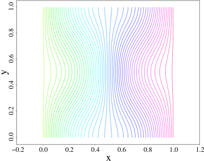
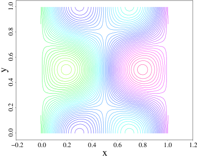
Figure 1: Left panel: flux function with $\delta=0.1$. Right panel: flux function with $\delta=0.5$.

As shown in Fig. 1, $\delta$ controls the magnetic field topology: for $\delta=0.1$ the magnetic field is simply connected, whereas for $\delta=0.5$ it features magnetic islands with separatrices, X-points, and O-points. The latter are special points satisfying $\nabla\psi=\mathbf{0}$, and are magnetic nulls when $B_{0}=0$.

We consider a steady-state temperature field of the form:

$$T_{\infty}(x,y)=T_{\mathcal{N}}(\psi)+\epsilon\>\tilde{T}(x,y).$$ (30)

Here, $\epsilon$ is the dimensionless anisotropy ratio, as defined above. This ansatz is consistent with the asymptotic properties of the temperature field as $\epsilon\rightarrow 0$, Eq. 5. In particular, we choose $T_{\mathcal{N}}(\psi)=\psi$ and $\tilde{T}=\cos(4\pi y)\sin(4\psi x)$. This choice is consistent with the boundary conditions, and guarantees that $\nabla_{\parallel}^{2}\tilde{T}\not=0$.

The manufactured solution source is found by inserting the prescribed steady-state temperature (Eq. 30) into the steady-state transport equation, to find:

$$S=-(1-\epsilon)\nabla_{\parallel}^{2}\tilde{T}-\epsilon\nabla^{2}\tilde{T}-\nabla^{2}T_{\mathcal{N}}(\psi).$$ (31)

The explicit evaluation of the source is given in A. We note that this particular source is singular when magnetic nulls with $B=0$ are present (e.g., for $B_{0}=0$ and $\delta=0.5$). This will have implications for spatial convergence, as we shall see.

We have performed tests for $\epsilon=10^{-2},10^{-4},10^{-6}$, $\delta=0.1,0.5$, and various choices for $B_{0}$. Simulations are initialized using the analytical steady-state solution, and are run to numerical steady state to assess spatial accuracy (note that the temporal convergence properties of the semi-Lagrangian scheme have been assessed elsewhere [1, 2]). For all simulations, we use a BDF1 timestep $\Delta t=10^{-3}$ (normalized to $\chi_{\perp}$, which is comparable or larger to what would be typical in an evolving B-field context, e.g., magnetohydrodynamics) and run them until the error saturates, usually for 100 to 200 steps. Absolute errors are computed as an $\ell_{2}$-norm of the difference between the numerical solution and the analytical one, Eq. 30,

$$\mathrm{Error}=\sum_{i,j}\Delta x_{i}\Delta y_{j}(T_{ij}-T_{\infty}(x_{i},y_{j}))^{2}.$$ (32)

5.1 Convergence study of the tokamak-ordering formulation

We begin with a mesh convergence study of the tokamak-ordering formulation with the null-space solution, i.e., $\tilde{T}=0$, which is insensitive to the magnetic-field topology (since the $\nabla_{\parallel}$ operator is annihilated). This test is intended to confirm the expected spatial discretization accuracy (fourth-order), and has been performed with $\delta=0.1,0.5$ and with $B_{0}=0$ (i.e., no guide field). The results are shown in Fig 2, and confirm the expected fourth-order accuracy scaling.

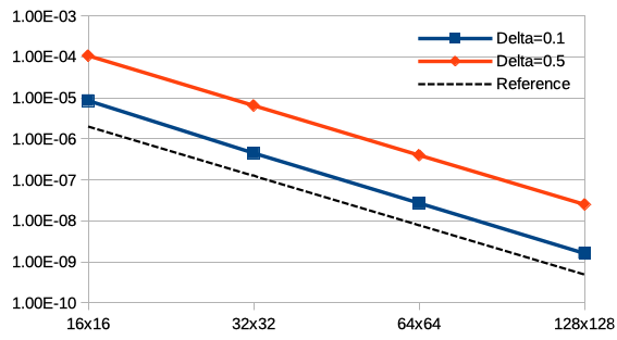
Figure 2: Mesh convergence study for the tokamak-ordering formulation with a null-space solution ($\tilde{T}=0$) for $\epsilon=10^{-2}$ with $B_{0}=0$ and $\delta=0.1,0.5$. Fourth-order spatial convergence is achieved, as expected.

Next, we confirm that the tokamak-ordering formulation converges to the true analytical solution as the guide field $B_{0}$ is increased. We consider the case of $\delta=0.1$ and $\epsilon=10^{-2}$. The results are shown in Fig. 3-left.

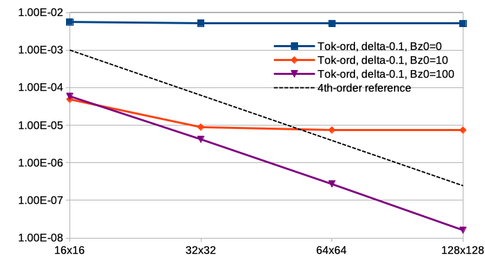
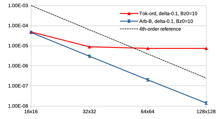
Figure 3: Mesh convergence study for the full solution with $\epsilon=10^{-2}$ and $\delta=0.1$. Left: tokamak-ordering formulation for three different guide fields, $B_{0}=0,10,100$, demonstrating convergence of the tokamak-ordering solution to the analytical one as the guide-field $B_{0}$ increases. Right: Comparison of errors between tokamak-ordering and arbitrary-B formulation for $B_{0}=10$, demonstrating the ability of the arbitrary-B formulation to converge where the tokamak-ordering one fails.

As expected, with $B_{0}=0$ there is a strong b-compressibility and the tokamak ordering approximation is unable to reproduce the temperature analytical solution regardless of mesh resolution. For a guide field of $B_{0}=10\gg B_{p}$, the error decreases as the mesh is refined for sufficiently coarse meshes, but it saturates for finer meshes when the spatial discretization error becomes smaller than that introduced by the tokamak-ordering approximation, which for the magnetic field in Eq. 28 is of $\mathcal{O}(B_{0}^{-3})$ (as is evident from the figure by inspecting the error saturation levels for different $B_{0}$). Increasing the guide field further to $B_{0}=100\ggg B_{p}$ results in fourth-order-accurate convergence for all meshes considered, although the scaling is expected to break at some point for further refined meshes.

5.2 Convergence study of the arbitrary-B formulation

In contrast, the new arbitrary-B formulation is able to recover convergence with the analytical solution for arbitrary guide-field strength $B_{0}$ and mesh resolution. For sufficiently large guide fields compared to $B_{p}$, $B_{0}=10$, Fig. 3-right shows (for $\epsilon=10^{-2}$) that, unlike the tokamak-ordering formulation, the new arbitrary-B formulation produces the expected fourth-order asymptotic convergence rate for all meshes considered.

Convergence results for guide fields $B_{0}\lesssim B_{p}$ (i.e., more compressible magnetic field topologies) are more nuanced. This is so because special magnetic-field topological surfaces such as separatrices (which separate closed and open field lines) become more relevant, impacting the accuracy of the simulation more.

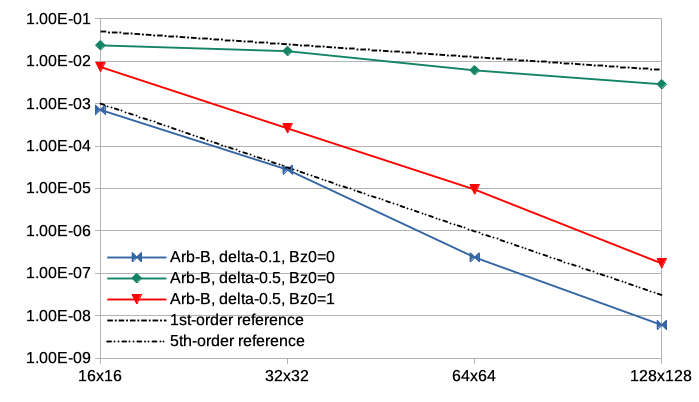
(a) $\epsilon=10^{-2}$

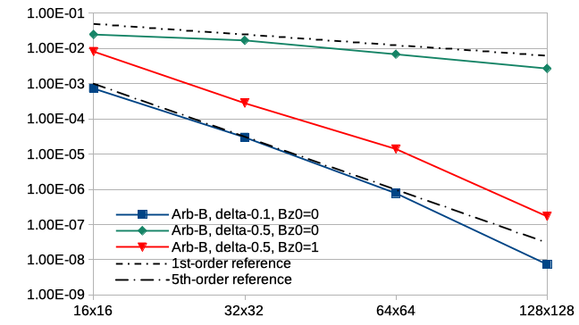
(b) $\epsilon=10^{-4}$

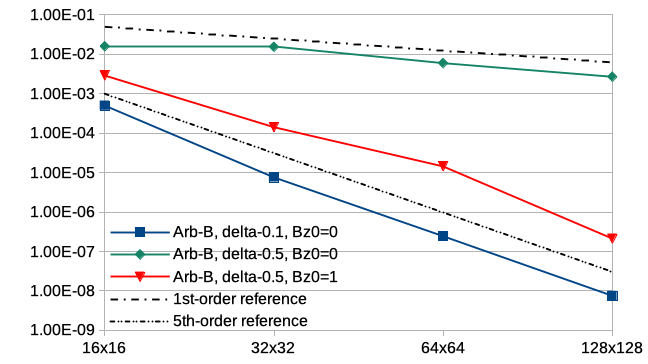
(c) $\epsilon=10^{-6}$

Figure 4: Mesh convergence study with the arbitrary-B formulation for small or zero magnetic guide fields.

Fig. 4 depicts convergence results for $\epsilon=10^{-2},10^{-4},10^{-6}$ and various combinations of $B_{0}=0,1$ and $\delta=0.1,0.5$. The first thing to notice is that error levels are largely independent of the anisotropy ratio $\epsilon$, as expected from an AP formulation [1, 2]. Secondly, we see order reduction of our numerical discretization to first-order accuracy for the $B_{0}=0$, $\delta=0.5$ case, for which the verification source is singular by construction due to the presence of magnetic nulls. This is a consequence of the particular choice of verification solution, and not a property of the method, which is otherwise able to deal with it seamlessly in a convergent manner.

In the cases where the verification source is regular but still with $B_{0}\lesssim B_{p}$ (e.g., $\delta=0.1$, $B_{0}=0$ or $\delta=0.5$, $B_{0}=1$), we actually find super-convergence with mesh refinement, of fifth-order instead of the expected fourth-order. Further inspection of the numerical errors for these cases (see Figs. 5a and 5b for $\epsilon=10^{-4}$) reveals that the errors for $B_{0}\lesssim B_{p}$ concentrate along one-dimensional manifolds, e.g. along the boundary for $\delta=0.1$ and around magnetic-island separatrices for $\delta=0.5$, which explains the super-convergence (since the $\ell_{2}$-norm accounts for volume elements in the computation of the errors, Eq. 32). These 1D manifolds are locations where boundary layers form, and where the numerical error is expected (and found) to be largest [1, 2]. The 1D error manifolds disappear as one increases the guide field sufficiently, as evidenced by Figs. 5c and 5d, which are obtained for $\epsilon=10^{-4}$ and $B_{0}=10\gg B_{p}$.

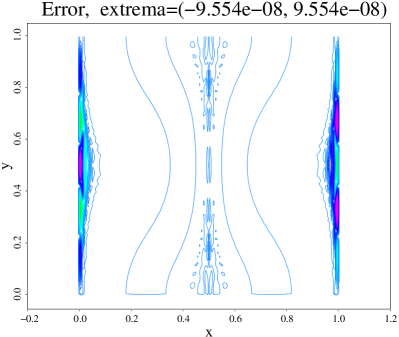
(a) $\delta=0.1$ and $B_{0}=0$

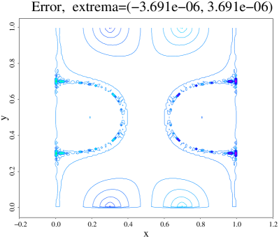
(b) $\delta=0.5$ and $B_{0}=1$

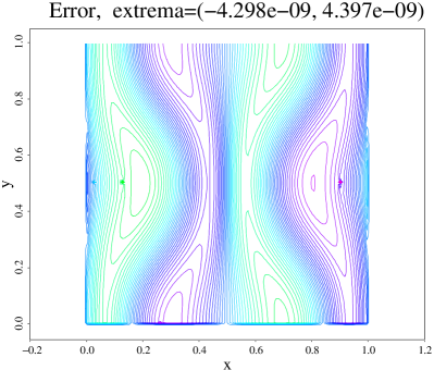
(c) $\delta=0.1$ and $B_{0}=10$

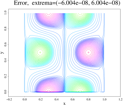
(d) $\delta=0.5$ and $B_{0}=10$

Figure 5: Steady-state errors vs the analytical solution for $\epsilon=10^{-4}$ on the $128\times 128$ mesh for various choices of $\delta$ and $B_{0}$.

6 Discussion and conclusions

We have proposed an extension of the recently proposed semi-Lagrangian formulation [1, 2] for the highly anisotropic heat transport equation to deal with arbitrary magnetic field configurations by lifting the so-called tokamak-ordering approximation, which required $\nabla\cdot(\mathbf{B}/B)\sim 0$. The new approach still leverages analytical Green’s functions for field-line integrals (which is critical to make the method tractable) by employing a suitable change of variables and introducing a suitable positive-definite field $\beta(\mathbf{x})$. A prescription for $\beta(\mathbf{x})$ is proposed that renders the discrete formulation consistent, AP, and able to deal with magnetic nulls seamlessly. The method has been verified with a manufactured solution for arbitrary guide fields and anisotropy ratios, and has been demonstrated to achieve at least fourth-order design spatial accuracy in all cases without magnetic field nulls. Magnetic field nulls render the verification solution source singular, resulting in order reduction to first order, but does not break the method. This order reduction is a consequence of the particular choice of verification solution rather than a feature of the method. Future extensions of this work will consider nonlinear heat transport coefficients and finite magnetic field lines, e.g. when magnetic field lines intersect the domain boundary.

Appendix A Manufactured solution source

The manufactured solution source is found from:

$$S=-(1-\epsilon)\nabla_{\parallel}^{2}\tilde{T}-\epsilon\nabla^{2}\tilde{T}-\nabla^{2}T_{\mathcal{N}}(\psi).$$ (33)

Using (per the main text) $T_{0}(\psi)=x+\delta\sin(2\pi x)\cos(2\pi y)$ and $\tilde{T}=\cos(4\pi y)\sin(4\psi x)$, we find:

$$\nabla^{2}\tilde{T} = -32\pi^{2}\sin(4\pi x)\cos(4\pi y)$$

$$\nabla^{2}T_{\mathcal{N}}(\psi) = -8\pi^{2}\delta\sin(2\pi x)\cos(2\pi y)$$

$$\nabla_{\parallel}^{2}\tilde{T} = 4\pi\Biggl{\{}-\frac{4\pi^{2}}{B^{2}}\biggl{(}\Bigl{(}B_{x}^{2}+B_{y}^{2}\Bigr{)}\cos(4\pi y)\sin(4\pi x)$$

$$+2B_{x}B_{y}\cos(4\pi x)\sin(4\pi y)\biggr{)}$$

$$+\;\cos(4\pi x)\cos(4\pi y)\left(\partial_{y}\left(\frac{B_{x}B_{y}}{B^{2}}\right)+\partial_{x}\left(\frac{B_{x}^{2}}{B^{2}}\right)\right)$$

$$-\;\sin(4\pi x)\sin(4\pi y)\left(\partial_{x}\left(\frac{B_{x}B_{y}}{B^{2}}\right)+\partial_{y}\left(\frac{B_{y}^{2}}{B^{2}}\right)\right)\Biggr{\}}.$$

The derivative terms read:

$$\partial_{x}\left(\frac{B_{x}^{2}}{B^{2}}\right) = 2\mathcal{A}B_{x}\biggl{\{}\cos(2\pi x)\sin(2\pi y)\left(1-\frac{B_{x}}{B^{2}}\right)$$

$$+\sin(2\pi x)\cos(2\pi y)\frac{B_{x}B_{y}}{B^{2}}\biggr{\}}$$

$$\partial_{x}\left(\frac{B_{x}B_{y}}{B^{2}}\right) = \mathcal{A}\Biggl{\{}B_{y}\cos(2\pi x)\sin(2\pi y)\left(1-2\frac{B_{x}^{2}}{B^{2}}\right)$$

$$-B_{x}\cos(2\pi y)\sin(2\pi x)\left(1-2\frac{B_{y}^{2}}{B^{2}}\right)\Biggr{\}}$$

$$\partial_{y}\left(\frac{B_{y}^{2}}{B^{2}}\right) = 2\mathcal{A}B_{y}\biggl{\{}\sin(2\pi y)\cos(2\pi x)\left(\frac{B_{y}^{2}}{B^{2}}-1\right)$$

$$-\cos(2\pi y)\sin(2\pi x)\frac{B_{x}B_{y}}{B^{2}}\biggr{\}}$$

$$\partial_{y}\left(\frac{B_{x}B_{y}}{B^{2}}\right) = \mathcal{A}\Biggl{\{}B_{y}\cos(2\pi y)\sin(2\pi x)\left(1-\frac{2B_{x}^{2}}{B^{2}}\right)$$

$$-B_{x}\cos(2\pi x)\sin(2\pi y)\left(1-\frac{2B_{y}^{2}}{B^{2}}\right)\Biggr{\}},$$

with $\mathcal{A}=\frac{4\pi^{2}\delta}{B^{2}}$ . Note that the source is singular for magnetic nulls, $B=0$.

Appendix B Error of the operator-split arbitrary-B Lagrangian formulation

An operator-split algorithm can be formulated from the formal result in Eq. 20 as suggested in Ref. [1] by considering first an update of the slow dynamics (which exactly respects the null space [1]):

$$\frac{T^{*}-T^{n}}{\Delta t}=\nabla_{\perp}^{2}T^{*}+S,$$ (34)

followed by a Lagrangian step in which the new-time temperature in the source $S^{*}$ (Eq. 19) is approximated by $T^{*}$. It follows that $S^{*}=\beta\frac{T^{*}-T^{n}}{\Delta t},$ and hence the Lagrangian splitting stage simply reads:

$$T_{OS}^{n+1}(\mathbf{x}) = \mathcal{G}_{\lambda}\left(T^{n};\mathbf{x},\frac{\Delta t}{\beta\epsilon}\right)+\mathcal{P}_{\lambda}\left(T^{*}-T^{n};\mathbf{x},\frac{\Delta t}{\beta\epsilon}\right)+\mathcal{E}_{split},$$ (35)

which is otherwise identical to the one proposed in Ref. [1] except for the parameter $\beta$, and the fact that the Lagrangian integrals are performed in the variable $\lambda$.

However, as formulated, this operator-split algorithm is not convergent with either small $\Delta t$ or small $\epsilon$. This can be readily shown by computing the operator-splitting local-truncation error (LTE) by subtracting Eqs. 35 and 20, which can be written after some manipulation as:

$$\mathcal{E}_{split}=T^{n+1}-T_{OS}^{n+1}\approx\mathcal{P}_{\lambda}\left((T^{n+1}-T^{*})-\frac{T^{n+1}-T^{n}-\Delta t(\nabla_{\perp}^{2}T^{n+1}+S)}{\beta B^{2}};\mathbf{x},\frac{\Delta t}{\beta\epsilon}\right).$$

Using the BDF1 semi-discretization of the original transport PDE, we can write this result as:

$$\mathcal{E}_{split}=T^{n+1}-T_{OS}^{n+1}\approx\mathcal{P}_{\lambda}\left((T^{n+1}-T^{*})-\frac{\Delta t}{\epsilon\beta}\partial_{\lambda}^{2}T^{n+1};\mathbf{x},\frac{\Delta t}{\beta\epsilon}\right).$$

For the first splitting-error contribution, $\mathcal{P}_{\lambda}\left(T^{n+1}-T^{*};\mathbf{x},\frac{\Delta t}{\beta\epsilon}\right)$, a Fourier analysis yields (following Ref. [1]):

$$\hat{\mathcal{E}}_{split,I}^{k_{\parallel}}\sim\hat{T}_{k_{\parallel}}\Delta t\min\left[1,\frac{k_{\parallel}^{2}\Delta t}{\epsilon}\right],$$

which is convergent in all regimes of $\Delta t/\epsilon$. However, for the second contribution, we have:

$$\mathcal{E}_{split,II}=\frac{\Delta t}{\epsilon\beta}\mathcal{P}_{\lambda}\left(\partial_{\lambda}^{2}T^{n+1};\mathbf{x},\frac{\Delta t}{\beta\epsilon}\right)=\mathcal{G}_{\lambda}\left(T^{n+1};\mathbf{x},\frac{\Delta t}{\beta\epsilon}\right),$$

which follows by integration by parts of the kernel integral and using that $\partial_{s}^{2}\mathcal{U}(s,t)=\frac{1}{t}G(s,t)$. Therefore, we find:

$$\mathcal{E}_{split,II}=\mathcal{G}_{\lambda}\left(T^{n+1};\mathbf{x},\frac{\Delta t}{\beta\epsilon}\right)\rightarrow\begin{cases}T^{n+1}(\mathbf{x}),&\Delta t\ll\beta\epsilon\\ \left\langle T^{n+1}\right\rangle,&\Delta t\gg\beta\epsilon\end{cases},$$

which does not vanish with either arbitrarily small $\Delta t$ or $\epsilon$, and is therefore not convergent.

References

- [1] L. Chacón, D. del Castillo-Negrete, and C. D. Hauck, “An asymptotic-preserving semi-lagrangian algorithm for the time-dependent anisotropic heat transport equation,” Journal of Computational Physics, vol. 272, pp. 719–746, 2014.
- [2] O. Koshkarov and L. Chacón, “A fully implicit, asymptotic-preserving, semi-lagrangian algorithm for the time dependent anisotropic heat transport equation,” Journal of Computational Physics, 2024. submitted.
- [3] D. del Castillo-Negrete and L. Chacón, “Local and nonlocal parallel heat transport in general magnetic fields,” Physical review letters, vol. 106, no. 19, p. 195004, 2011.
- [4] D. del Castillo-Negrete and L. Chacón, “Parallel heat transport in integrable and chaotic magnetic fields,” Physics of Plasmas, vol. 19, no. 5, p. 056112, 2012.
- [5] S. Braginskii, “Transport phenomena in plasma,” Reviews of plasma physics, vol. 1, p. 205, 1963.
- [6] M. Hölzl, S. Günter, I. Classen, Q. Yu, E. Delabie, T. Team, et al., “Determination of the heat diffusion anisotropy by comparing measured and simulated electron temperature profiles across magnetic islands,” Nuclear fusion, vol. 49, no. 11, p. 115009, 2009.
- [7] C. Ren, J. D. Callen, T. A. Gianakon, C. C. Hegna, Z. Chang, E. D. Fredrickson, K. M. McGuire, G. Taylor, and M. C. Zarnstorff, “Measuring ’ from electron temperature fluctuations in the Tokamak Fusion Test Reactor,” Physics of Plasmas, vol. 5, no. 2, pp. 450–454, 1998.
- [8] J. Meskat, H. Zohm, G. Gantenbein, S. Günter, M. Maraschek, W. Suttrop, Q. Yu, and A. U. Team, “Analysis of the structure of neoclassical tearing modes in ASDEX Upgrade,” Plasma Physics and Controlled Fusion, vol. 43, no. 10, p. 1325, 2001.
- [9] J. Snape, K. Gibson, T. O’gorman, N. Barratt, K. Imada, H. Wilson, G. Tallents, I. Chapman, et al., “The influence of finite radial transport on the structure and evolution of m/n= 2/1 neoclassical tearing modes on MAST,” Plasma Physics and Controlled Fusion, vol. 54, no. 8, p. 085001, 2012.
- [10] M. J. Choi, G. S. Yun, W. Lee, H. K. Park, Y.-S. Park, S. A. Sabbagh, K. J. Gibson, C. Bowman, C. W. Domier, N. C. Luhmann Jr, et al., “Improved accuracy in the estimation of the tearing mode stability parameters (’ and ) using 2D ECEI data in KSTAR,” Nuclear Fusion, vol. 54, no. 8, p. 083010, 2014.
- [11] K. Salari and P. Knupp, “Code verification by the method of manufactured solutions,” tech. rep., Sandia National Lab.(SNL-NM), Albuquerque, NM (United States), 2000.
- [12] L. Chacon, D. Daniel, and W. T. Taitano, “An asymptotic-preserving 2d-2p relativistic drift-kinetic-equation solver for runaway electron simulations in axisymmetric tokamaks,” Journal of Computational Physics, vol. 449, p. 110772, 2022.