Charge transport in a junction with a precessing anisotropic molecular spin - negative shot noise at zero-bias voltage

Abstract

Anisotropic molecular magnets can be employed to manipulate charge transport in molecular nanojunctions. The charge transport through an electronic level connected to source and drain contacts and exchange-coupled with a precessing anisotropic molecular spin in an external magnetic field is studied here. Both the magnetic field and the uniaxial magnetic anisotropy parameter of the molecular spin control the total precession frequency. The Keldysh nonequilibrium Green’s functions method is used to derive expressions for charge current and current noise. The precessing molecular magnetization drives inelastic tunnelling processes between electronic quasienergy levels. The dc-bias voltages allow to unveil the quasienergy levels, Larmor frequency and the anisotropy parameter, through characteristics of charge-transport measurements involving steps and peak-dip features. Under zero-bias voltage conditions, negative correlations of opposite-spin currents lead to negative shot noise for a sufficiently large anisotropy parameter that enables the change of the precession direction with respect to Larmor precession. Furthermore, it is possible to adjust the magnetic anisotropy parameter to suppress the precession frequency, leading to the suppression of shot noise. The results show that in the given setup, the charge current and shot noise can be controlled by the uniaxial magnetic anisotropy of the molecular magnet.

I Introduction

Single-molecule magnets have gained much attention since the beginning of the new century due to the possibility to be used as constituent elements in spintronic devices for high-density information storage and quantum information processing.m1 ; m2 ; m3 ; m4 ; m5 ; m6 The key role in these applications plays the uniaxial magnetic anisotropy, characterized by parameter $D$, which leads to the bistability of the molecular spin states, with two degenerate ground states $\pm S$, separated by an energy barrier to spin reversal $DS^{2}$ (for integer spins) at low temperatures.m2 ; m3 ; m7 ; m8 Depending on the sign of the anisotropy parameter, there are two types of uniaxial anisotropy: easy-axis ($D>0$), and easy-plane ($D<0$) anisotropy.m2 For successful applications in magnetic storage, the energy barrier needs to be enhanced,m9 but its increase cannot be accomplished by a simultaneous increase of the anisotropy parameter $D$ and the ground state spin $S$, and the only way to control the barrier height it to modulate the value of $D$.m10 ; m11 ; m12 ; m13 On the other hand, in-plane and small magnetic anisotropy is desirable for applications in quantum information processing.m14 In order to design magnetic molecules with desired characteristics, learning to control and manipulate the magnetic anisotropy parameter $D$ is essential.

Charge transport through magnetic molecules has been studied both theoreticallyt1 ; t2 ; we2013 ; t3 ; t31 ; t4 ; t5 ; t6 ; t7 ; t8 and experimentally.e1 ; e2 ; e3 ; manipulation1 ; e4 ; e5 ; e6 ; e7 The studies have addressed various phenomena, such as e.g., Kondo effect,kondo1 ; kondo2 ; kondo3 ; kondo4 Pauly spin blockade,spinblockade1 ; spinblockade2 ; spinblockade3 Coulomb blockade,e1 ; coulombblockade1 ; coulombblockade2 ; coulombblockade3 molecular magnetization switching induced by electric currentbodecurrentinduced or in contact with a superconducting lead,superconductor and spin-dependent Seebeck and Peltier effect.seebeck1 ; seebeck2 ; seebeck3 ; seebeck4 The possibility to manipulate molecular magnetization by charge current has already been demonstrated experimentally.e2 ; e3 ; manipulation1 ; e4 ; e5 ; manipulation2 It has been theoretically predicted that exchange interactions between molecular magnets can be electrically controlled.t3 ; t31 Magnetic anisotropy can be varied and controlled by various means such as, electrical current,t1 ; coulombblockade2 ; an1 ; an2 ; an3 ; an4 electric field,coulombblockade2 ; ele1 ; ele2 ; ele3 ; ele4 molecular mechanical stretching,stretching and by ligand substitution.ligsub High anisotropy barriers for spin reversal were observed in some isolated metal complexes, but due to their reactivity and instability, they are not suitable candidates to be exploited in magnetic storage.metal1 ; metal2 ; metal3 ; metal4 Also, new optical techniques of spin readout in single-molecule magnets have been investigated recently.opt1 ; opt2 ; opt3

The nonequilibrium Green’s functions techniqueJauho1993 ; Jauho1994 ; JauhoBook has been used to derive various characteristics of quantum transport through single molecules and molecular magnets, such as charge current, current-current correlations, spin current, inelastic transport, heat current, etc.t2 ; t3 ; t31 ; t4 ; seebeck4 ; innoiz1 ; neg1 ; neg2 ; t41 ; neg3 Charge-current noise in transport junctions arising from the discreteness of charge of conducting electrons is an exciting topic in nanophysics, since it can give us additional information about charge transport which is hidden from the current measurements.Blanter2024 Within the framework of nonequilibrium Green’s functions technique, the effect of inelastic transport on shot noise has been studied,innoiz1 ; innoiz2 ; innoiz3 ; innoiz4 ; we2018 as well as current fluctuations in the transient regime.transient It has been shown previously that spin-flip can lead to suppressioninnoiz2 ; noises or enhancementnoisee1 ; noisee2 of the shot noise. The shot noise has been employed to give information on the e.g., energy of transmission channels,Blanter2024 fractional charges,fractional2024 and Cooper pairs.Cooper2024 Recently, the nonequilibrium noise due to temperature gradient at zero-bias voltage has become an active research topic.grad1 ; grad2 ; grad3 ; grad4 ; grad5 Moreover, it has been demonstrated that negative values of this noise are a sign of spin-flip scattering due to temperature bias.grad6

The goal of this article is to theoretically study the charge transport through a single electronic energy level that may be an orbital of a molecular magnet or belong to a nearby quantum dot, in the presence of a precessing anisotropic molecular spin in a constant external magnetic field, connected to electric contacts. The precession frequency is contributed by the Larmor precession frequency and the uniaxial magnetic anisotropy parameter of the molecular spin, and kept undamped by external means. The spin of the itinerant electron in the electronic level and the molecular spin are coupled via exchange interaction. The charge current and current noise are calculated by means of the Keldysh nonequilibrium Green’s functions technique.Jauho1993 ; Jauho1994 ; JauhoBook The shot noise of charge current is a result of the competition between correlations of currents with the same spins and correlations of currents with the opposite spins. Both elastic tunnelling, driven by the dc-bias voltage, and inelastic tunnelling, driven by the precessional motion of the anisotropic molecular spin, contribute to the charge transport. It is shown that by proper tuning of the uniaxial magnetic anisotropy parameter, the charge-current shot noise can be manipulated and reduced. The energies of the channels available for electron transport are Floquet quasienergies, which are obtained by the Floquet theorem.Floquet1 ; Floquet2 ; Floquet3 ; Floquet4 They are dependent on the magnetic anisotropy of the molecular spin and can be varied accordingly. Both charge current and shot noise are saturated for sufficiently large magnetic anisotropy parameter. Similarly to our previous work where the precessing molecular spin was isotropic,we2018 the peak-dip features in the shot noise are manifestations of the destructive quantum interferenceinterf2024 between the states connected with inelastic tunnelling, here involving absorption(emission) of an energy which is linearly dependent on the uniaxial anisotropy parameter. Finally, the negative shot noise at zero-bias conditions and zero temperature, as a key result of this work, is a manifestation of the dominance of the negative correlations between currents with opposite spins, for chemical potentials that enable inelastic tunnelling processes accompanied with spin-flips of itinerant electrons, only if the anisotropy parameter is sufficiently large to change the direction of the molecular spin precession with respect to the external magnetic field. Moreover, the uniaxial magnetic anisotropy parameter can suppress the precession frequency of the molecular magnetization, leading to zero shot noise.

The rest of the article is arranged in the following way. The model setup of the system is described in Sec. II. Theoretical formalism used to derive the results is given in Sec. III. The expressions for the charge current and the current noise are calculated by means of the Keldysh nonequilibrium Green’s functions method.Jauho1993 ; Jauho1994 ; JauhoBook The results are shown and discussed in Sec. IV, where the effects of the uniaxial magnetic anisotropy of the molecular spin on the charge-transport properties at zero temperture are analysed. This section is followed by Sec. V in which the conclusions are presented.

II Model Setup

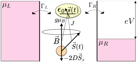
Figure 1: (Color online) Tunneling through a single molecular orbital with energy $\epsilon_{0}$ coupled to the anisotropic spin $\vec{S}(t)$ of a molecular magnet via exchange interaction with the coupling constant $J$, in the presence of a magnetic field $\vec{B}$, connected to two metallic leads with chemical potentials $\mu_{L}$ and $\mu_{R}$. The applied bias voltage $eV=\mu_{L}-\mu_{R}$, with tunnel rates $\Gamma_{L}$ and $\Gamma_{R}$, and the uniaxial anisotropy constant of the molecular magnet $D$. The spin of the molecule precesses around the magnetic field axis with modified frequency $\omega=\omega_{L}-2DS_{z}$.

The junction under consideration consists of a single molecular orbital of a molecular magnet, in the presence of a constant external magnetic field along $z$-axis, $\vec{B}=B\vec{e}_{z}$, coupled to two noninteracting metallic leads (see Fig. 1). The leads with chemical potentials $\mu_{L}$ (left) and $\mu_{R}$ (right) are unaffected by the magnetic field. The Hamiltonian describing the junction is given by $\hat{H}=\hat{H}_{L}+\hat{H}_{R}+\hat{H}_{T}+\hat{H}_{MO}+\hat{H}_{S}$. Here, the Hamiltonian of lead $\xi=L,R$ can be written as $\hat{H}_{\xi}=\sum_{k,\sigma}\epsilon_{k\xi}\hat{c}^{\dagger}_{k\sigma\xi}\hat{c}_{k\sigma\xi}$. The subscript $\sigma=\uparrow,\downarrow=1,2=\pm 1$ denotes the spin-up or spin-down state of the electrons. The tunnel coupling between the molecular orbital and the leads is introduced by $\hat{H}_{T}=\sum_{k,\sigma,\xi}[V_{k\xi}\hat{c}^{\dagger}_{k\sigma\xi}\hat{d}_{\sigma}+V^{\ast}_{k\xi}\hat{d}^{\dagger}_{\sigma}\hat{c}_{k\sigma\xi}]$, with matrix element $V_{k\xi}$. Here, $\hat{c}^{\dagger}_{k\sigma\xi}(\hat{c}_{k\sigma\xi})$ and $\hat{d}^{\dagger}_{\sigma}(\hat{d}_{\sigma})$ denote the creation (annihilation) operators of the electrons in the leads and the molecular orbital. The Hamiltonian of the molecular orbital is given by $\hat{H}_{MO}=\sum_{{\sigma}}\epsilon_{0}\hat{d}^{\dagger}_{\sigma}\hat{d}_{\sigma}+(g\mu_{B}/\hbar)\hat{\vec{s}}\vec{B}+J\hat{\vec{s}}\hat{\vec{S}}$, where the first term is the Hamiltonian of the noninteracting molecular orbital with energy $\epsilon_{0}$. The second term describes the electronic spin in the molecular orbital, $\hat{\vec{s}}=(\hbar/2)\sum_{\sigma\sigma^{\prime}}(\hat{\vec{\sigma}})_{\sigma\sigma^{\prime}}\hat{d}^{\dagger}_{\sigma}\hat{d}_{\sigma^{\prime}}$, in the presence of the magnetic field $\vec{B}$. The vector of the Pauli matrices is given by $\hat{\vec{\sigma}}=(\hat{\sigma}_{x},\hat{\sigma}_{y},\hat{\sigma}_{z})^{T}$, while $g$ and $\mu_{B}$ are the gyromagnetic ratio of the electron and the Bohr magneton. The third term in the Hamiltonian of the orbital represents the exchange interaction between the electronic spin and the spin of the magnetic molecule, where $J$ is the constant of the exchange coupling. The term $\hat{H}_{S}=g\mu_{B}{\hat{\vec{S}}}{\vec{B}}-D\hat{S^{2}_{z}}$ represents the Hamiltonian of the anisotropic molecular spin $\hat{\vec{S}}=\hat{S_{x}}\vec{e}_{x}+\hat{S_{y}}\vec{e}_{y}+\hat{S_{z}}\vec{e}_{z}$, where $D$ is the uniaxial magnetic anisotropy constant. We assume for simplicity, that $g$ factor of the molecular spin equals that of a free electron.

Assuming that the spin of the molecular magnet is large and that it can be considered as a classical variable $\vec{S}$, with constant length $S=\textbar{\vec{S}}\textbar\gg\hbar$, where $\vec{S}=\langle\hat{\vec{S}}\rangle$ is the expectation value of the molecular spin operator, its dynamics is given by the Heisenberg equation of motion $\dot{\vec{S}}=\big{\langle}\dot{\hat{\vec{S}}}\big{\rangle}\ =(i/\hbar)\big{\langle}\big{[}\hat{H},\hat{\vec{S}}\big{]}\big{\rangle}$. Neglecting the quantum fluctuations and using external means, such as radiofrequency fields,Kittel to compensate for the loss of the molecular magnetic energy due to its interaction with the itinerant electrons, so that the molecular spin dynamics remains unaffected by the exchange interaction, the equation $\dot{\vec{S}}=g\mu_{B}\vec{B}\times\vec{S}-2D\vec{S}_{z}\times\vec{S}$ is obtained. The molecular spin precesses around $z$-axis, with frequency $\omega=\omega_{L}-2DS_{z}$, where $\omega_{L}=g\mu_{B}B$ is the Larmor precession frequency in the external magnetic field $\vec{B}$, while $-2DS_{z}$ is the contribution of the uniaxial anisotropy to the precession frequency $\omega$. The motion of the molecular spin is then given by $\vec{S}(t)=S_{\bot}\cos(\omega t)\vec{e}_{x}+S_{\bot}\sin(\omega t)\vec{e}_{y}+S_{z}\vec{e}_{z}$, where $\theta$ is the tilt angle between $z$-axis and $\vec{S}$, $S_{\bot}=S\sin(\theta)$ and $S_{z}=S\cos(\theta)$. Although the motion of the molecular spin is kept precessional externally,Kittel the molecular magnet itself pumps charge current into the leads, thus affecting the transport properties of the junction.

III Theoretical Formalism

III.1 Charge Current

The charge-current operator of the contact $\xi$ is given by the Heisenberg equation JauhoBook ; Jauho1994

$$\hat{I}_{\xi}(t)=-e\frac{d\hat{N}_{\xi}}{dt}=-e\frac{i}{\hbar}[\hat{H},\hat{N}_{\xi}],$$ (1)

where $\hat{N}_{\xi}=\sum_{{k,\sigma}}\hat{c}^{\dagger}_{k\sigma\xi}\hat{c}_{k\sigma\xi}$ represents the charge occupation number operator of the contact $\xi$, while $[\ ,\ ]$ denotes the commutator. The average charge current from the lead $\xi$ to the molecular orbital is then given by

$$I_{\xi}(t)=-e\bigg{\langle}\frac{d}{dt}\hat{N}_{\xi}\bigg{\rangle}\ =-e\frac{i}{\hbar}\big{\langle}\big{[}\hat{H},\hat{N}_{\xi}\big{]}\big{\rangle}.$$ (2)

Using the Keldysh nonequilibrium Green’s functions technique, the charge current can be calculated as Jauho1994 ; JauhoBook

$$I_{\xi}{(t)}= {2e}\ {\rm Re}\int dt^{\prime}{\rm Tr}\big{\{}{\hat{G}}^{r}{(t,t^{\prime})}{\hat{\Sigma}}^{<}_{\xi}(t^{\prime},t)$$

$$\quad\quad\quad\quad\quad\quad+{\hat{G}}^{<}{(t,t^{\prime})}{\hat{\Sigma}}^{a}_{\xi}(t^{\prime},t)\big{\}},$$ (3)

in units in which $\hbar=e=1$. The retarded, advanced, lesser and greater self-energies from the tunnel coupling between the molecular orbital and contact $\xi$ are denoted by $\hat{\Sigma}^{r,a,<,>}_{\xi}(t,t^{\prime})$. Their matrix elements are diagonal in the electron spin space with respect to the basis of the eigenstates of $\hat{s}_{z}$, with nonzero matrix elements given by $\Sigma^{r,a,<}_{\xi}(t,t^{\prime})=\sum_{{k}}V_{k\xi}^{\phantom{\ast}}g^{r,a,<,>}_{k\xi}{(t,t^{\prime})}V^{\ast}_{k\xi}$, where $g^{r,a,<,>}_{k\xi}{(t,t^{\prime})}$ represent the retarded, advanced, lesser and greater Green’s functions of the electrons in the lead $\xi$. The Green’s functions of the electrons in the molecular orbital are given by $\hat{G}^{r,a,<,>}(t,t^{\prime})$, with matrix elements $G^{r,a}_{\sigma\sigma^{\prime}}{(t,t^{\prime})}=\mp i\theta(\pm t\mp t^{\prime})\langle\{\hat{d}_{\sigma}{(t)},\hat{d}^{\dagger}_{\sigma^{\prime}}{(t^{\prime})}\}\rangle$, while $G^{<}_{\sigma\sigma^{\prime}}(t,t^{\prime})=i\langle\hat{d}^{\dagger}_{\sigma^{\prime}}(t^{\prime})\hat{d}_{\sigma}(t)\rangle$ and $G^{>}_{\sigma\sigma^{\prime}}(t,t^{\prime})=-i\langle\hat{d}_{\sigma}(t)\hat{d}^{\dagger}_{\sigma^{\prime}}(t^{\prime})\rangle$, where $\{\cdot,\cdot\}$ denotes the anticommutator. Applying the double Fourier transformations in Eq. (3), one obtains

$$I_{\xi}{(t)}= \,-2e\Gamma_{\xi}{\rm Im}\int\frac{d\epsilon}{2\pi}\int\frac{d\epsilon^{\prime}}{2\pi}e^{-i(\epsilon-\epsilon^{\prime})t}$$

$$\times{\rm Tr}\bigg{\{}f_{\xi}(\epsilon^{\prime}){\hat{G}}^{r}{(\epsilon,\epsilon^{\prime})+{\frac{1}{2}{\hat{G}}^{<}}{(\epsilon,\epsilon^{\prime})}}\bigg{\}},$$ (4)

where the tunnel coupling between the molecular orbital and contact $\xi$, $\Gamma_{\xi}(\epsilon)=2\pi\sum_{{k}}\lvert V_{k\xi}\rvert^{2}\delta(\epsilon-\epsilon_{k\xi})$, is energy independent in the wide-band limit and considered constant. The Fermi-Dirac distribution of the electrons in the lead $\xi$ is given by $f_{\xi}(\epsilon)=[e^{(\epsilon-\mu_{\xi})/k_{B}T}+1]^{-1}$, with $k_{B}$ the Boltzmann constant and $T$ the temperature.

The matrix components of the retarded Green’s function $\hat{G}^{r}$ of the electrons in the molecular orbital, can be obtained by applying Dyson’s expansion and analytic continuation rules.JauhoBook Their double Fourier transforms readGuo ; we2016

$$G^{r}_{\sigma\sigma}(\epsilon,\epsilon^{\prime}) =\frac{2\pi\delta(\epsilon-\epsilon^{\prime})G^{0r}_{\sigma\sigma}(\epsilon)}{1-\gamma^{2}G^{0r}_{\sigma\sigma}(\epsilon){G^{0r}_{-\sigma-\sigma}(\epsilon_{\sigma})}},$$ (5)

$$G^{r}_{\sigma-\sigma}(\epsilon,\epsilon^{\prime}) =\frac{2\pi\gamma\delta(\epsilon_{\sigma}-\epsilon^{\prime})G^{0r}_{\sigma\sigma}(\epsilon)G^{0r}_{-\sigma-\sigma}(\epsilon_{\sigma})}{1-\gamma^{2}G^{0r}_{\sigma\sigma}(\epsilon)G^{0r}_{-\sigma-\sigma}(\epsilon_{\sigma})},$$ (6)

where the abbreviation $\epsilon_{\sigma}=\epsilon-\sigma\omega=\epsilon-\sigma(\omega_{L}-2DS_{z})$ is used, and $\gamma=JS\sin(\theta)/2$. Applying the double Fourier transformations to the Keldysh equation, the lesser and greater Green’s functions can be calculated as $\hat{G}^{<,>}(\epsilon,\epsilon^{\prime})=\int d\epsilon^{\prime\prime}\hat{G}^{r}(\epsilon,\epsilon^{\prime\prime})\hat{\Sigma}^{<,>}(\epsilon^{\prime\prime})\hat{G}^{a}(\epsilon^{\prime\prime},\epsilon^{\prime})/2\pi$.JauhoBook , where ${\Sigma}^{<}(\epsilon)=i\sum_{\xi}\Gamma_{\xi}f_{\xi}(\epsilon)$, ${\Sigma}^{>}(\epsilon)=i\sum_{\xi}\Gamma_{\xi}(f_{\xi}(\epsilon)-1)$ and $\hat{G}^{a}(\epsilon,\epsilon^{\prime})=[\hat{G}^{r}(\epsilon^{\prime},\epsilon)]^{\dagger}$. The retarded Green’s function $\hat{G}^{0r}$ of the electrons in the orbital in the presence of only the static spin component $S_{z}$ along the axis of the external magnetic field can be found using the equation of motion technique,Bruus and after applying the Fourier transformations, one writes $\hat{G}^{0r}(\epsilon)=[\epsilon-\epsilon_{0}-\Sigma^{r}-\hat{\sigma}_{z}(g\mu_{B}B+JS_{z})/2]^{-1}$,Guo ; bodecurrentinduced where $\Sigma^{r,a}=\mp i\Gamma/2$ and $\Gamma=\sum_{\xi}\Gamma_{\xi}$. Finally, using Eqs. (4)-(6), and obtaining $\hat{G}^{<}(\epsilon,\epsilon^{\prime})$ from the Keldysh equation, the average charge current from the contact $\xi$ can be written as

$$I_{\xi} =\frac{e\Gamma_{\xi}\Gamma_{\zeta}}{\hbar}\int\frac{d\epsilon}{2\pi}[f_{\xi}(\epsilon)-f_{\zeta}(\epsilon)]$$

$$\times\sum_{\begin{subarray}{c}\sigma\sigma^{\prime}\\ \sigma\neq\sigma^{\prime}\end{subarray}}\frac{\lvert G^{0r}_{\sigma\sigma}(\epsilon)\rvert^{2}[1+\gamma^{2}\lvert G^{0r}_{\sigma^{\prime}\sigma^{\prime}}(\epsilon+\sigma^{\prime}\omega_{L}-2\sigma^{\prime}DS_{z})\rvert^{2}]}{\lvert 1-\gamma^{2}G^{0r}_{\sigma\sigma}(\epsilon)G^{0r}_{\sigma^{\prime}\sigma^{\prime}}(\epsilon+\sigma^{\prime}\omega_{L}-2\sigma^{\prime}DS_{z})\rvert^{2}},$$ (7)

with $\xi\neq\zeta$. In the limit $DS_{z}\ll\omega_{L}$, Eq. (7) reduces to the previously calculated expression for the charge current.we2018

III.2 Density of States in the Molecular Orbital

The positions of the resonant transmission channels available for electron transport in the molecular orbital can be obtained from the density of states in the molecular orbital

$$\rho(\epsilon)=-\frac{1}{\pi}\sum_{\sigma=\pm 1}{\rm Im}\bigg{\{}\frac{G^{0r}_{\sigma\sigma}(\epsilon)}{1-\gamma^{2}G^{0r}_{\sigma\sigma}(\epsilon)G^{0r}_{-\sigma-\sigma}(\epsilon_{\sigma})}\bigg{\}}.$$ (8)

Taking into account that the Hamiltonian of the molecular orbital is a periodic function of time $\hat{H}_{MO}(t)=\hat{H}_{MO}(t+\mathcal{T})$, with $\mathcal{T}=2\pi/\omega$, the Floquet quasienergy levels $\epsilon_{i}$, $i=1,2,3,4$, at which the resonant transmission channels are located, can be calculated using the Floquet theorem.Floquet1 ; Floquet2 ; Floquet3 ; Floquet4 As the Floquet Hamiltonian matrix is block diagonal, for quasienergies within the interval $[0,\omega)$ a block is given by

$$\left(\begin{array}[]{cc}\lambda_{1}-\omega&JS_{\bot}/2\\ \vspace*{-0.1cm}\hfil\\ JS_{\bot}/2&\lambda_{2}\end{array}\right),$$ (9)

where $\lambda_{1,2}=\epsilon_{0}\pm(\omega_{L}+JS_{z})/2$. The eigenvalues of the matrix (9) are quasienergy levels $\epsilon_{1}$ and $\epsilon_{3}$, while $\epsilon_{2}=\epsilon_{1}+\omega$ and $\epsilon_{4}=\epsilon_{3}+\omega$. They are given by

$$\epsilon_{1,3}=\epsilon_{0}-\frac{\omega_{L}}{2}+ DS_{z}\pm\sqrt{D(D+J)S^{2}_{z}+\bigg{(}\frac{JS}{2}\bigg{)}^{2}},$$ (10)

$$\epsilon_{2,4}=\epsilon_{0}+\frac{\omega_{L}}{2}- DS_{z}\pm\sqrt{D(D+J)S^{2}_{z}+\bigg{(}\frac{JS}{2}\bigg{)}^{2}}.$$ (11)

In the molecular orbital, an electron with energy $\epsilon_{1}(\epsilon_{2})$ or $\epsilon_{3}(\epsilon_{4})$ can absorb (emit) energy equal to one energy quantum $\omega$ due to the precessional motion of the anisotropic molecular spin, ending up in the quasienergy level with energy $\epsilon_{2}(\epsilon_{1})$ or $\epsilon_{4}(\epsilon_{3})$ , so that the state with quasienergy $\epsilon_{1}(\epsilon_{3})$ is coupled with the state with quasienergy $\epsilon_{2}(\epsilon_{4})$.

III.3 Noise of Charge Current

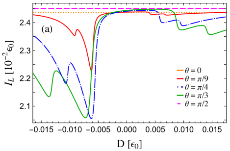
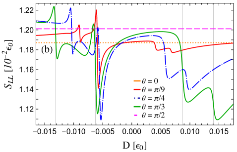
Figure 2: (Color online) (a) Charge current $I_{L}$ and (b) autocorrelation shot noise $S_{LL}$ as functions of the uniaxial magnetic anisotropy parameter $D$ for different tilt angles $\theta$, at zero temperature, with $\vec{B}=B\vec{e}_{z}$. The chemical potentials of the leads are equal to: $\mu_{L}=\nobreak 2.5\,\epsilon_{0}$ and $\mu_{R}=0$. The other parameters are set to: $\Gamma=\nobreak 0.05\,\epsilon{0},\,\Gamma_{L}=\Gamma_{R}=\Gamma/2,\,\omega_{L}=\nobreak 0.5\,\epsilon_{0},\,J=\nobreak 0.01\,\epsilon_{0},\,S=100$. Grid lines related to the noise function $S_{LL}$ for $\theta=\pi/3$ (green line), are positioned at $D=-0.01312\,\epsilon_{0}$ ($\mu_{L}=\epsilon_{2}$), $D=-0.00625\,\epsilon_{0}$ ($\mu_{R}=\epsilon_{3}$), $D=0.00875\,\epsilon_{0}$ ($\mu_{R}=\epsilon_{4}$), and $D=0.01406\,\epsilon_{0}$ ($\mu_{L}=\epsilon_{1}$).

Additional properties of the charge transport in the junction can be obtained by analysing the charge-current noise. In view of the fact that the nonzero commutator in Eq. (1) is generated by the tunnelling Hamiltonian $\hat{H}_{T}$, the charge current operator $\hat{I}_{\xi}(t)$ can be written as

$$\hat{I}_{\xi}(t)=e\frac{i}{\hbar}\sum_{\sigma}\hat{I}_{\xi\sigma}(t),$$ (12)

with the operator component $\hat{I}_{\xi\sigma}(t)$ given by

$$\hat{I}_{\xi\sigma}(t)=\sum_{k}[V_{k\xi}\hat{c}^{{\dagger}}_{k\sigma\xi}(t)\hat{d}_{\sigma}(t)-V^{*}_{k\xi}\hat{d}^{{\dagger}}_{\sigma}(t)\hat{c}_{k\sigma\xi}(t)].$$ (13)

The fluctuation operator of the charge current in contact $\xi$ is given by

$$\delta\hat{I}_{\xi}(t)=\hat{I}_{\xi}(t)-\langle\hat{I}_{\xi}(t)\rangle.$$ (14)

The correlation between fluctuations of currents in leads ${\xi}$ and ${\zeta}$, known as nonsymmetrized charge-current noise is written asJauhoBook ; Blanter2024

$$S_{\xi\zeta}(t,t^{\prime})=\langle\delta\hat{I}_{\xi}(t)\delta\hat{I}_{\zeta}(t^{\prime})\rangle.$$ (15)

With the help of Eqs. (12)-(14), one obtains the noise as

$$S_{\xi\zeta}(t,t^{\prime})=-\frac{e^{2}}{\hbar^{2}}\sum_{\sigma\sigma^{\prime}}S^{\sigma\sigma^{\prime}}_{\xi\zeta}(t,t^{\prime}),$$ (16)

with $S^{\sigma\sigma^{\prime}}_{\xi\zeta}(t,t^{\prime})=\langle\delta\hat{I}_{\xi\sigma}(t)\delta\hat{I}_{\zeta\sigma^{\prime}}(t^{\prime})\rangle$. Applying Wick’s theoremWick2024 and Langreth analytical continuation rules,Langreth2024 the correlation functions $S^{\sigma\sigma^{\prime}}_{\xi\zeta}(t,t^{\prime})$ introduced in Eq. (16) can be calculated.JauhoBook ; transient Using the Fourier transforms of Green’s functions $G^{r,a,<,>}_{\sigma\sigma^{\prime}}(\epsilon,\epsilon^{\prime})$ and self-energies $\Sigma^{r,a,<,>}_{\xi}(\epsilon)$, the charge-current noise becomes

$$S_{\xi\zeta}(t,t^{\prime})=-\frac{e^{2}}{\hbar^{2}}\sum_{\sigma\sigma^{\prime}}\bigg{\{}\int \frac{d\epsilon_{1}}{2\pi}\int\frac{d\epsilon_{2}}{2\pi}\int\frac{d\epsilon_{3}}{2\pi}\int\frac{d\epsilon_{4}}{2\pi}e^{-i(\epsilon_{1}-\epsilon_{2})t}e^{i(\epsilon_{3}-\epsilon_{4})t^{\prime}}$$

$$\times \big{\{}[G^{r}_{\sigma\sigma^{\prime}}(\epsilon_{1},\epsilon_{3})\Sigma^{>}_{\zeta}(\epsilon_{3})+2G^{>}_{\sigma\sigma^{\prime}}(\epsilon_{1},\epsilon_{3})\Sigma^{a}_{\zeta}][G^{r}_{\sigma^{\prime}\sigma}(\epsilon_{4},\epsilon_{2})\Sigma^{<}_{\xi}(\epsilon_{2})+2G^{<}_{\sigma^{\prime}\sigma}(\epsilon_{4},\epsilon_{2})\Sigma^{a}_{\xi}]$$

$$+[\Sigma^{>}_{\xi}(\epsilon_{1})G^{a}_{\sigma\sigma^{\prime}}(\epsilon_{1},\epsilon_{3})+2G^{>}_{\sigma\sigma^{\prime}}(\epsilon_{1},\epsilon_{3})\Sigma^{r}_{\xi}][\Sigma^{<}_{\zeta}(\epsilon_{4})G^{a}_{\sigma^{\prime}\sigma}(\epsilon_{4},\epsilon_{2})+2G^{<}_{\sigma^{\prime}\sigma}(\epsilon_{4},\epsilon_{2})\Sigma^{r}_{\zeta}]$$

$$+4\Sigma^{r}_{\xi}\Sigma^{a}_{\zeta}G^{>}_{\sigma\sigma^{\prime}}(\epsilon_{1},\epsilon_{3})G^{<}_{\sigma^{\prime}\sigma}(\epsilon_{4},\epsilon_{2})\big{\}}$$

$$-\delta_{\xi\zeta}\delta_{\sigma\sigma^{\prime}}\int\frac{d\epsilon_{1}}{2\pi}\int\frac{d\epsilon_{2}}{2\pi}\int\frac{d\epsilon_{3}}{2\pi}$$

$$\hskip 11.38092pt\times\big{\{}e^{-i(\epsilon_{1}-\epsilon_{3})t}e^{i(\epsilon_{2}-\epsilon_{3})t^{\prime}}G^{>}_{\sigma\sigma^{\prime}}(\epsilon_{1},\epsilon_{2})\Sigma^{<}_{\xi}(\epsilon_{3})$$

$$\hskip 11.38092pt+e^{-i(\epsilon_{1}-\epsilon_{3})t}e^{i(\epsilon_{1}-\epsilon_{2})t^{\prime}}\Sigma^{>}_{\xi}(\epsilon_{1})G^{<}_{\sigma^{\prime}\sigma}(\epsilon_{2},\epsilon_{3})\big{\}}\bigg{\}}.$$ (17)

The resulting noise depends only on the time difference $\tau=t-t^{\prime}$, and its power spectrum is given by

$$S_{\xi\zeta}(\Omega)=\int d\tau e^{i\Omega\tau}S_{\xi\zeta}(\tau).$$ (18)

The charge current given by Eq. (7) is conserved, implying that the zero-frequency ($\Omega=0$) noise power satisfies the relations $S_{LL}(0)=S_{RR}(0)=-S_{LR}(0)=-S_{RL}(0)$. In experimental configurations zero-frequency noise power spectrum is standardly measured. In the remainder of this article, the zero-frequency noise power $S_{LL}=S_{LL}(0)$ at zero temperature will be discussed, as in this particular case it is contributed only by the shot noise, while thermal noise vanishes.

IV Results

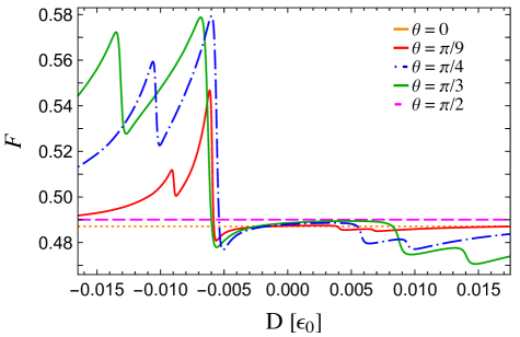
Figure 3: (Color online) Fano factor $F$ as a function of the uniaxial anisotropy parameter $D$. The plots are obtained for different tilt angles $\theta$ at zero temperature, with $\vec{B}=B\vec{e}_{z}$. The chemical potentials of the leads are equal to: $\mu_{L}=\nobreak 2.5\,\epsilon_{0}$ and $\mu_{R}=0$. The other parameters are set to: $\Gamma=\nobreak 0.05\,\epsilon{0},\,\Gamma_{L}=\Gamma_{R}=\Gamma/2,\,\omega_{L}=\nobreak 0.5\,\epsilon_{0},\,J=\nobreak 0.01\,\epsilon_{0},\,S=100$.

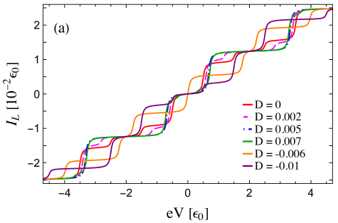
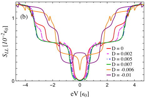
Figure 4: (Color online) (a) Charge current $I_{L}$ and (b) autocorrelation shot noise $S_{LL}$ as functions of the applied bias voltage $eV=\mu_{L}-\mu_{R}$ with $\mu_{L,R}=\pm eV/2$ and $\vec{B}=B\vec{e}_{z}$, for different uniaxial magnetic anisotropy parameters $D$ at zero temperature. The other parameters are set to: $\Gamma=\nobreak 0.05\,\epsilon{0},\,\Gamma_{L}=\Gamma_{R}=\Gamma/2,\,\omega_{L}=\nobreak 0.5\,\epsilon_{0},\,J=\nobreak 0.01\,\epsilon_{0},\,S=100$, and $\theta=\pi/3$. All energies are given in the units of $\epsilon_{0}$. The steps in the noise function $S_{LL}$ correspond to resonances $\mu_{\xi}=\epsilon_{1,3}$, with $\xi=L,R$. As manifestations of the quantum interference effect, the dip-peak characteristics for $eV<0$ correspond to $\mu_{R}=\epsilon_{2,4}$, while the peak-dip characteristics for $eV>0$ correspond to $\mu_{L}=\epsilon_{2,4}$.

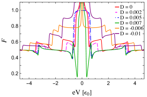
Figure 5: (Color online) Fano factor $F$ as a function of the applied bias voltage $eV=\mu_{L}-\mu_{R}$ with $\mu_{L,R}=\pm eV/2$ and $\vec{B}=B\vec{e}_{z}$, for different uniaxial magnetic anisotropy parameters $D$ at zero temperature. The other parameters are set to: $\Gamma=\nobreak 0.05\,\epsilon{0},\,\Gamma_{L}=\Gamma_{R}=\Gamma/2,\,\omega_{L}=\nobreak 0.5\,\epsilon_{0},\,J=\nobreak 0.01\,\epsilon_{0},\,S=100$, and $\theta=\pi/3$. All energies are given in the units of $\epsilon_{0}$.

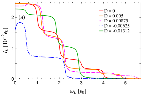
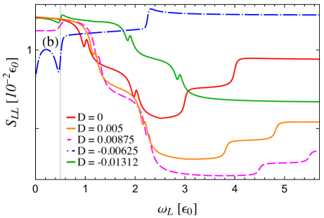
Figure 6: (Color online) (a) Charge current $I_{L}$ and (b) autocorrelation shot noise $S_{LL}$ as functions of the Larmor frequency $\omega_{L}$ for different uniaxial magnetic anisotropy parameters $D$. All plots are obtained at zero temperature with $\vec{B}=B\vec{e}_{z}$. The chemical potentials of the leads are equal to: $\mu_{R}=0$ and $\mu_{L}=\nobreak 2.5\,\epsilon_{0}$, except for $D=-0.00625\,\epsilon_{0}$, where $\mu_{L}=1.125\,\epsilon_{0}$. The other parameters are set to: $\Gamma=\nobreak 0.05\,\epsilon{0},\,\Gamma_{L}=\Gamma_{R}=\Gamma/2,\,J=\nobreak 0.01\,\epsilon_{0},\,S=100$, and $\theta=\pi/3$. All energies are given in the units of $\epsilon_{0}$. All steps in the current $I_{L}$, and the corresponding steps and dip-peak features in the noise $S_{LL}$, denote a resonance $\mu_{\xi}=\epsilon_{i}$, with $\xi=L,R$. A distinct dip in the noise $S_{LL}$ appears for $D=-0.00625\,\epsilon_{0}$ (blue dot-dashed line) around $\omega_{L}=0.5\,\epsilon_{0}$ (grid line), and a significant drop of the corresponding current due to the double resonance: $\mu_{R}=\epsilon_{3}$ and $\mu_{L}=\epsilon_{4}$.

Now we analyse the behaviour of the charge current $I_{L}$, noise power $S_{LL}$, and Fano factor $F=S_{LL}/e|I_{L}|$ as functions of the uniaxial magnetic anisotropy parameter $D$, bias voltage $eV=\mu_{L}-\mu_{R}$, and Larmor frequency $\omega_{L}$ (magnetic field $B$), focusing on the influence of the tuning anisotropy parameter $D$ on the transport properties of the system. In particular, it will be shown that the anisotropy parameter $D$ can contribute to the controlling and reducing the noise power. One should emphasize that the shot noise is the result of the competition between the predominantly positive contribution coming from the correlations of currents with the same spins, and predominantly negative contribution of correlations between charge currents with opposite spins.

In Fig. 2 the average charge current from the left lead $I_{L}$ and autocorrelation shot noise $S_{LL}$ are presented as functions of the uniaxial anisotropy parameter $D$, for five different tilt angles $\theta$, while the corresponding Fano factor $F$ is shown in Fig. 3. The fano factor $F<1$, so the noise is sub-Poissonian. Immediately, we see that the current, shot noise and consequently the Fano factor are constant for $\theta=0$ (orange, dotted lines) and $\theta=\pi/2$ (pink, dashed lines). If we look at the expression for the current, given by Eq. (7), we notice that for $\theta=0$, $\gamma=0$ as well and the charge current dependence on $D$ vanishes. On the other hand, for $\theta=\pi/2$, the $z$-component of the molecular spin $S_{z}=0$, and hence the current does not depend on the anisotropy parameter $D$ either. For the tilt angle $\theta=\pi/3$ (green line) and $D=-0.01312\,\epsilon_{0}$ [grid line in Fig. 2(b)], corresponding to $\mu_{L}=\epsilon_{2}=2.5\,\epsilon_{0}$, there is a dip-peak feature in the current and a peak-dip feature in the shot noise and Fano factor. Similarly as in the Fano effect,Fano2024 the peak-dip characteristics are a manifestation of the destructive quantum interference between the states connected with inelastic tunneling processes involving absorption(emission) of an energy quantum $\omega$. Namely, there are two tunnelling processes, one elastic through quasienergy level with energy e.g. $\epsilon_{1}$, and the other inelastic through the quasienergy level $\epsilon_{2}=\epsilon_{1}+\omega$, involving the emission of the amount energy $\omega$ and ending up in the same level $\epsilon_{1}$. The two tunnelling pathways destructively interfere and negatively contribute to the shot noise. For this set of parameters, only quasienergy level with energy $\epsilon_{3}=-0.5\,\epsilon_{0}$ lies out of the bias-voltage window. However, as the anisotropy parameter $D$ increases, the quasienergy level $\epsilon_{3}$ moves up the energy scale and enters the bias-voltage window for $D=-0.00625$ [another grid line in Fig. 2(b)], with $\mu_{R}=\epsilon_{3}=0$. In this case, all four levels lie within the bias-voltage window, leading to the enhancement of the current after its minimum value, and the most prominent peak-dip feature in the noise and Fano factor. With further increase of the anisotropy parameter $D$, the current and noise approach constant values, and $F\approx 0.49$, but since the quasienergy level $\epsilon_{4}$ moves down the energy scale, for $D=0.00875$ [the third grid line in Fig. 2(b)], it reaches the resonance with $\mu_{R}$, i.e., $\mu_{R}=\epsilon_{4}=0$, leading to the decrease of current and shot noise when 3 quasienergy levels remain within the bias-voltage window. For $D=0.01406$ [the remaining grid line in Fig. 2(b)], the quasienergy level $\epsilon_{1}$ which increases with the increase of $D$, is in resonance with $\mu_{L}$, i.e., $\mu_{L}=\epsilon_{1}$, before it leaves the bias-voltage window with further increase of $D$, resulting in the final peak-dip feature in the charge current and shot noise, where the dip in the noise represents its minimum value. For $\theta=\pi/4$ [blue dot-dashed lines in Fig. 2] one notices that both charge current and shot noise have minimum values around the value of anisotropy parameter $D$ that corresponds to the entrance of all four quasienergy levels into the bias-voltage window. Both charge current and shot noise are saturated for large values of $\lvert D\rvert$.

The average charge current $I_{L}$ as a function of the applied bias-voltage $eV$ at zero temperature is plotted for six different values of anisotropy parameter $D$ in Fig. 4(a), where the bias voltage is varied such that $\mu_{L,R}=\pm eV/2$. As the bias voltage increases, a new channel available for electron transport, with an energy $\epsilon_{i}$, $i\in\{1,2,3,4\}$, enters the bias-voltage window, resulting in a step increase in the current. Since the positions of the quasienergy levels $\epsilon_{i}$ depend on molecular spin anisotropy, for different values of $D$, the staircase current function will show steps at different values of $eV$. The shot noise of charge current $S_{LL}$ is shown in Fig.4(b). The step-like characteristics in the noise power correspond to resonances $\mu_{\xi}=\pm eV/2=\epsilon_{1,3}$, while peak-dip characteristics for $eV>0$ and dip-peak characteristics for $eV<0$ as manifestations of the quantum interference effect, correspond to resonances $\mu_{\xi}=\pm eV/2=\epsilon_{2,4}$, with $\xi=L,R$. Hence, they change their positions with the change of the anisotropy parameter $D$. For the given set of parameters: $\omega_{L}=0.5\epsilon_{0}$, $\theta=\pi/3$, and $D=0.005\epsilon_{0}$ in Fig. 4 (blue, dot-dashed line), one obtains $\omega=\omega_{L}-DS=0$ and there are only two transport channels in this case, with energies $\epsilon=0.34\epsilon_{0}$ and $\epsilon\prime=1.66\epsilon_{0}$, available for the elastic tunnelling, denoted by the steps at $\pm eV/2=\epsilon$ and $\pm eV/2=\epsilon\prime$. The current is equal to zero for $eV=0$, but the noise power is contributed by the inelastic processes in which an electron absorbs an energy $\omega$, leading to the divergence of the Fano factor [see Fig. 5]. The noise becomes sub-Poissonian ($F<1$) as soon as one of the levels $\epsilon_{i}$ enters the bias-voltage window, since the transmission probability increases. After all the levels $\epsilon_{i}$ enter the bias-voltage window, the Fano factor becomes constant $F=1/2$.fanohalf In the case of only elastic tunnelling ($D=0.005$, $\omega=0$, blue dot-dashed line), the Fano factor $F=1$ for $0<eV<\epsilon$, since the transmission probability is very low and the currents remain uncorrelated until the first channel available for transport appears. For $D=0.007$ (green line), one notices sharp dips in the Fano factor at $eV=0.32\epsilon_{0}$, while in the relevant noise plot a small peak-dip feature can be noticed. This corresponds to the level $\epsilon_{4}$ entering the bias-voltage window, i.e., $\mu_{L}=\epsilon_{4}$, leading to the destructive quantum interference. We notice another peak-dip feature due to the quantum interference effect on the same line at $eV=3.28\epsilon_{0}$, corresponding to $\mu_{L}=\epsilon_{2}$. The other step-like and peak-dip features in Fig. 5 denote energies of the available transport channels $\epsilon_{i}=\pm eV/2$.

The average charge current $I_{L}$ and noise $S_{LL}$ as functions of $\omega_{L}$ at zero temperature, for several different values of the magnetic anisotropy parameter $D$, are shown in Figs. 6(a) and 6(b). Here, the bias voltage is varied as $eV=\mu_{L}-\mu_{R}$, with $\mu_{R}=0$, while $\mu_{L}=2.5\epsilon_{0}$, except for the blue dot-dashed lines where $\mu_{L}=1.125\epsilon_{0}$. All steps in the current $I_{L}$, as well as steps and dip-peak features in the noise $S_{LL}$, correspond to a resonance $\mu_{\xi}=\epsilon_{i}$. The dip-peak features are a result of the competition between positive correlations of the currents with the same spin, and negative correlations of the currents with the opposite spins, with an impact of the quantum interference effect for the interfering tunnelling pathways. For $\omega_{L}=0$, $D=-0.00625\epsilon_{0}$ and $\mu_{L}=1.25\epsilon_{0}$ [Fig. 6 (blue dot-dashed lines)], both current and noise increase, since quasienergy level $\epsilon_{1}$ enters the bias-voltage window, $\mu_{L}=\epsilon_{1}$, while $\epsilon_{2}=1.75\epsilon_{0}$, $\epsilon_{3}=0.25\epsilon_{0}$ and $\epsilon_{4}=0.875\epsilon_{0}$. In Fig. 6(b), around $\omega_{L}=0.5\epsilon_{0}$ (grid line), one observes a step-like increase for $D=0.00875$ (pink line), due to the fact that $\epsilon_{4}=\mu_{R}$, while for $D=-0.01312$ there is a dip-peak structure, as $\mu_{L}=\epsilon_{2}$, showing the impact of the destructive quantum interference effect (green line), and for $D=-0.00625$, the two chemical potentials $\mu_{R}$ and $\mu_{L}$ are in resonance with two levels connected with spin-flip events, $\epsilon_{3}$ and $\epsilon_{4}$, resulting in a dip with higher magnitude (blue dot-dashed line). Here, due to the destructive interference effect, the negative contribution of the correlations between the currents with opposite spins shows a dip-peak structure, while the positive correlations of the charge currents with the electrons spin-up shows a positive dip, resulting in the higher dip in the noise $S_{LL}$ around $\omega_{L}=0.5\epsilon_{0}$. In all the plots in Fig. 6, for $\omega_{L}$ and $D$ such that one remaining quasienergy level $\epsilon_{i}$ within the bias-voltage window is in resonance with the chemical potential of one of the leads, one notices the final step decrease in the current $I_{L}$, and the final step increase in $S_{LL}$ (red, orange, pink dashed, and blue dot-dashed line) or a dip-peak structure (green line). For $D=-0.0625\epsilon_{0}$ and $\omega_{L}=2.25\epsilon_{0}$ (blue dot-dashed line) the remaining level within the bias-voltage window $\epsilon_{1}$ is in resonance with $\mu_{R}$, $\epsilon_{1}=\mu_{R}$, whereas, e.g., for $D=-0.01312\epsilon_{0}$ and $\omega_{L}=2.87\epsilon_{0}$ (green line), the energy of the only level within the bias-voltage window equals $\epsilon_{4}=\mu_{L}$. With further increase of $\omega_{L}$, all for levels $\epsilon_{i}$ lie out of the bias-voltage window and the current $I_{L}\rightarrow 0$, while the noise power becomes a constant due to the inelastic processes, and the Fano factor $F$ presented in Fig. 7 indicates the super-Poissonian noise, $F>1$. Again, one can see that $F\rightarrow 1/2$ if all the quasienergy levels lie within the bias voltage window,fanohalf e.g., for $D=0.005\epsilon_{0}$ and $\omega\leq 1.18\epsilon_{0}$ (orange line), while the Fano factor $F$ slightly increases with the increase of $\omega_{L}$, since three levels remain within the bias voltage window, and the noise is sub-Poissonian. With further increase of $\omega_{L}$ the two levels $\epsilon_{1}$ and $\epsilon_{4}$ remain within the bias-voltage window, and the uncorrelated currents lead to $F\rightarrow 1$. Finally, with only one quasienergy level within the bias-voltage window, the current decreases and the noise becomes super-Poissonian. For $D=-0.00625\epsilon_{0}$ (blue dot-dashed line) the noise becomes super-Poissonian already around $\omega_{L}=0.5\epsilon_{0}$, since for $0.5\epsilon_{0}<\omega_{L}\leq 2.25\epsilon_{0}$ only level $\epsilon_{1}$ lies within the bias-voltage window.

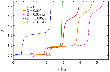
Figure 7: (Color online) Fano factor $F$ as a function of the Larmor frequency $\omega_{L}$ for different uniaxial magnetic anisotropy parameters $D$. All plots are obtained at zero temperature with $\vec{B}=B\vec{e}_{z}$. The chemical potentials of the leads are equal to: $\mu_{R}=0$ and $\mu_{L}=\nobreak 2.5\,\epsilon_{0}$, except for $D=-0.00625$ (blue dot-dashed line), where $\mu_{L}=1.125\,\epsilon_{0}$. The other parameters are set to: $\Gamma=\nobreak 0.05\,\epsilon{0},\,\Gamma_{L}=\Gamma_{R}=\Gamma/2,\,J=\nobreak 0.01\,\epsilon_{0},\,S=100$, and $\theta=\pi/3$. All energies are given in the units of $\epsilon_{0}$.

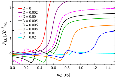
Figure 8: (Color online) Shot noise of charge current $S_{LL}$ as a function of the Larmor frequency $\omega_{L}$ for different uniaxial magnetic anisotropy parameters $D$ at zero-bias voltage. All plots are obtained at zero temperature with $\vec{B}=B\vec{e}_{z}$. The chemical potentials of the leads are equal and set to: $\mu_{L}=\mu_{R}=0.25\,\epsilon_{0}$. The other parameters are set to: $\Gamma=\nobreak 0.05\,\epsilon{0},\,\Gamma_{L}=\Gamma_{R}=\Gamma/2,\,J=\nobreak 0.01\,\epsilon_{0},\,S=100$, and $\theta=\pi/3$. All energies are given in the units of $\epsilon_{0}$. The noise $S_{LL}$ is negative in regions with dominant negative correlations of currents with opposite spins.

In Fig. 8 the dependence of the charge current noise $S_{LL}$ on frequency $\omega_{L}$ is plotted for several values of the uniaxial magnetic anisotropy parameter $D$ and equal chemical potentials of the leads, $\mu_{L}=\mu_{R}=\mu=0.25\epsilon_{0}$, at zero temperature. The correlations of charge currents with the same spin contribute positively to the noise $S_{LL}$. However, due to the dominantly negative contribution of correlations between currents with opposite spins, the charge current noise $S_{LL}$, as a result of the competition between these two influences, is negative at some values of $\omega_{L}$ only for nonzero anisotropy $D\neq 0$. The negative shot noise has not been found previously,we2018 since in the case of the isotropic molecular spin with $D=0$ (red line in Fig. 8), noise $S_{LL}$ is an even, positive function of $\omega_{L}$ for $eV=0$, $S_{LL}(\omega_{L})=S_{LL}(-\omega_{L})$. In all the plots each step-like increase correspond to a resonance between chemical potential of the leads and one of the levels available for electron transport (some are not shown). For instance, if we take $\omega_{L}=0.5\epsilon_{0}$ (marked by a vertical grid line), there is a step-like increase for $D=0$ (red line) since the chemical potential $\mu$ is in resonance with level $\epsilon_{3}$, $\mu=\epsilon_{3}$. Similar step for $D=0.002\epsilon_{0}$ occurs around $\omega_{L}=0.586\epsilon_{0}$, where $\mu=\epsilon_{3}$ (purple line). For $\omega_{L}=0.5\epsilon_{0}$ and $D=0.005\epsilon_{0}$, the resulting $\omega=0$, with only two levels available for charge transport since $\epsilon_{1}=\epsilon_{2}$, $\epsilon_{3}=\epsilon_{4}$, and the charge current noise monotonically decreases around $\omega_{L}=0.5\epsilon_{0}$, drops to zero at $\omega_{L}=0.5\epsilon_{0}$, then monotonically increases (intersection between grid line and black line). Similarly, the charge current noise $S_{LL}$ is equal to zero for $\omega_{L}=0.8$, $D=0.008\epsilon_{0}$ (orange line) and for $\omega_{L}=\epsilon_{0}$, $D=0.01\epsilon_{0}$ (blue dot-dashed line). For $D=0.006\epsilon_{0}$, one observes negative noise if $\omega_{L}<0.5\epsilon_{0}$ , contributed by the correlations of charge currents with opposite spins. Here, $\mu=\epsilon_{4}$ at $\omega_{L}=0.5\epsilon_{0}$ and the destructive quantum interference takes place between levels $\epsilon_{3}$ and $\epsilon_{4}$, leading to the dip-peak feature around $\omega_{L}=0.5\epsilon_{0}$ (intersection between grid line and green line). Similarly, the destructive quantum interference effect can be observed e.g. around $\omega_{L}=0.322\epsilon_{0}$ (black line), or $\omega_{L}=0.149\epsilon_{0}$ (pink dashed line), where $\mu=\epsilon_{4}$. With further increase of the anisotropy parameter $D$, the noise $S_{LL}$ approaches zero (cyan line).

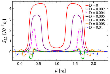
Figure 9: (Color online) Shot noise of charge current $S_{LL}$ at zero-current conditions, as a function of the chemical potential of the leads $\mu=\mu_{L}=\mu_{R}$, for different axial magnetic anisotropy parameters $D$. All plots are obtained at zero temperature with $\vec{B}=B\vec{e}_{z}$. The other parameters are set to: $\Gamma=\nobreak 0.05\,\epsilon{0},\,\Gamma_{L}=\Gamma_{R}=\Gamma/2,\,J=\nobreak 0.01\,\epsilon_{0},\,S=100$, Larmor frequency $\omega_{L}=0.5\,\epsilon_{0}$, and $\theta=\pi/3$. All energies are given in the units of $\epsilon_{0}$. The shot noise $S_{LL}$ is negative between levels connected with spin-flips for $\omega<0$, i.e., $D>\omega_{L}/S$.

The shot noise of charge current $S_{LL}$ as a function of chemical potential of the leads $\mu=\mu_{L}=\mu_{R}$ for several values of $D$ and $\omega_{L}=0.5\epsilon_{0}$ at zero temperature is shown in Fig. 9. The noise $S_{LL}$ takes positive values for $\omega=\omega_{L}-DS>0$, i.e., for $D<\omega_{L}/S$ in the regions between quasienergy levels connected with spin-flip events, taking into account the level broadening $\Gamma$ (see red, purple and pink dashed lines). The grid line in Fig. 9 at $\mu=0.25\epsilon_{0}$, corresponding to the grid line in Fig. 8 at $\omega_{L}=0.5\epsilon_{0}$, intersects with all the plots showing the suppression of the positive charge current noise with the increase of the anisotropy parameter $D$. The noise drops to zero for $\omega=0$, when the anisotropy constant $D=\omega_{L}/S=0.005\epsilon_{0}$ (black line in Fig. 9). With further increase of the anisotropy parameter $D$, the frequency $\omega<0$, the anisotropy parameter $D>\omega_{L}/S$, and the noise becomes negative between levels connected with spin-flip events (green, orange and blue dot-dashed lines). This is a pure contribution of correlations between charge currents with the opposite spins, since correlations of currents with the same spins drop to zero for $\omega\leq 0$. With further increase of the anisotropy, for a sufficiently large parameter $D$, the noise $S_{LL}$ becomes entirely suppressed and drops to zero.

V Conclusions

In this article, the characteristics of charge transport through a single molecular orbital in the presence of a precessing anisotropic molecular spin in a magnetic field, connected to two noninteracting metallic leads, was theoretically studied. The Larmor frequency is modified by a term with the uniaxial magnetic anisotropy parameter of the molecular spin, and the resulting precession with frequency $\omega=\omega_{L}-2DS_{z}$ is externally kept undamped. The expressions for charge current and current noise were obtained using the Keldysh nonequilibrium Green’s functions method.

The results show rich transport characteristics at zero temperature. The quantum interference between the states connected with precession-assisted inelastic tunnelling, involving absorption(emission) of an energy $\omega$, result in peak-dip (dip-peak) features in the shot noise. Each resonance between a chemical potential and an anisotropy dependent quasienergy level is visible in a transport measurement in the form of a step, peak-dip (dip-peak) or dip feature, and can be varied by tuning the anisotropy. For the most part the correlations between the same-spin (opposite-spin) currents are positive (negative). These negative correlations are particularly interesting at zero-bias conditions since in that case, the resulting shot noise is negative for chemical potentials between couples of quasienergy levels which are connected by the precession-assisted inelastic tunnelling, if the uniaxial anisotropy parameter of the molecular magnet is large enough to change the precession direction of the molecular magnetization with respect to the Larmor precession. Additionally, the magnetic anisotropy parameter can be adjusted to suppress the precession frequency, so that the resulting shot noise vanishes. It was shown that the charge current and shot noise can be controlled by a proper adjustment of the magnetic anisotropy parameter of the molecular magnet and reach their saturation if this parameter takes large values.

Taking into consideration that the charge transport in the given setup with the anisotropic molecular magnet can be manipulated by the uniaxial magnetic anisotropy of the molecular spin, and other parameters, the results of this study may be useful in the field of single-molecule electronics and spintronics. It might be useful for magnetic storage applications to study the charge- and spin-transport properties using a setup with a molecular spin modelled as a quantum object in the future.

- (1) L. Thomas, F. Lionti, R. Ballou, D. Gatteschi, R. Sessoli, and B. Barbara, Nature 383, 145-147 (1996).
- (2) D. Gatteschi, R. Sessoli, and J. Villain, Molecular Nanomagnets, Oxford University Press, New York (2006).
- (3) L. Bogani and W. Wernsdorfer, Nature Mater. 7, 179-186 (2008).
- (4) C. Timm and M. Di Ventra, Phys. Rev B 86, 104427 (2012).
- (5) M. N. Leuenberger and D. Loss, Nature 410, 789-793 (2001).
- (6) R. E. P. Winpenny, Angew. Chem. Int. Ed., 47, 7992-7994 (2008).
- (7) R. Sessoli, D. Gatteschi, A. Caneschi, and M. A. Novak, Nature 365 141-143 (1993).
- (8) M. Misiorny and J. Barnaś, Phys. Rev. B 77, 172414 (2008).
- (9) M. Mannini, F. Pineider, P. Sainctavit, C. Danieli, E. Otero, C. Sciancalepore, A. M. Talarico, M-A. Arrio, A. Cornia, D. Gatteschi, and R. Sessoli, Nature Mater. 8, 194-197 (2009)
- (10) O. Waldmann, Inorg. Chem. 46, 10035-10037 (2007).
- (11) C. J. Milios, R. Inglis, R. Bogai, W. Wernsdorfer, A. Collins, S. Moggach, S. Parsons, S. P. Perlepes, G. Christou and E. K. Brechin, Chem. Commun., 3476-3478 (2007).
- (12) F. Neese and D. A. Pantazis, Faraday Discussions 148, 229-238 (2011).
- (13) Y.-S. Meng, S.-D. Jiang, B.-W. Wang, and S. Gao, Acc. Chem. Res. 49, 11, 2381-2389 (2016).
- (14) A. Chiesa, P. Santini, E. Garlatti, F. Luis, and S. Carreta, Rep. Prog. Phys. 87, 034501 (2024).
- (15) M. Misiorny, M. Hell, and M. R. Wegewijs, Nature Physics 9, 801-805 (2013).
- (16) P. Stadler, C. Holmqvist, and W. Belzig, Phys. Rev. B 88, 104512 (2013).
- (17) M. Filipović, C. Holmqvist, F. Haupt, and W. Belzig, Phys. Rev. B 87, 045426 (2013); 88, 119901 (2013).
- (18) J. Fransson, J. Ren, and J.-X. Zhy, Phys. Rev. Lett. 113, 257201 (2014).
- (19) T. Saygun, J. Bylin, H. Hammar, and J. Fransson, Nano Lett. 16, 2824-2829 (2016).
- (20) H. Hammar and J. Fransson, Phys. Rev. B 94, 054311 (2016).
- (21) A. Płomińska, M. Misiorny, and I. Weymann, EPL 121, 38006 (2018).
- (22) U. Bajpai and B. Nikolić, Phys. Rev. B 99, 134409 (2019).
- (23) Z. Zhang, Y. Wang, H. Wang, H. Liu, and L. Dong, Nanoscale. Res. Lett. 16, 77 (2021).
- (24) R. Smorka, M. Thoss, and M. Žonda, New. J. Phys. 26, 013056 (2024).
- (25) H. B. Heersche, Z. de Groot, J. A. Folk, H. S. J. van der Zant, C. Romeike, M.R. Wegewijs, L. Zobbi, D. Barreca, E. Tondello, and A. Cornia, Phys. Rev. Lett. 96, 206801 (2006).
- (26) J. R. Hauptmann, J. Paaske, and P. E. Lindelof, Nature Phys. 4, 373-376 (2008).
- (27) S. Loth, K. von Bergmann, M. Ternes, A. F. Otte, C. P. Lutz, and A. J. Heinrich, Nature Phys. 6, 340-344 (2010).
- (28) T. Komeda, H. Isshiki, J. Liu, Y.-F. Zhang, N. Lorente, K. Katoh, B. K. Breedlove, and M. Yamashita, Nat. Commun. 2, 217 (2011).
- (29) R. Vincent, S. Klyatskaya, M. Ruben, W. Wernsdorfer, and F. Balestro, Nature 488, 357-360 (2012).
- (30) F. D. Natterer, K. Yang, W. Paul, P. Willke, T. Choi, T. Greber, A. J. Heinrich, and C. P. Lutz, Nature 543, 226-228 (2017).
- (31) G. Czap, P. J. Wagner, F. Xue, L. Gu, J. Li, J. Yao, R. Q. Wu, and W. Ho, Science 364, 670 (2019).
- (32) T. Pei, J. O Thomas, S. Sopp, M.-Y. Tsang, N. Dotti, J. Baugh, N. F. Chilton, S. Cardona-Serra, A. Gaita-Ariño, H. L. Anderson, and L. Bogani, Nat. Commun. 13, 4506 (2022).
- (33) C. Romeike, M. R. Wegewijs, W. Hofstetter, and H. Schoeller, Phys. Rev. Lett 96, 196601 (2006).
- (34) F. Elste and C. Timm, Phys Rev. B 81, 024421 (2010).
- (35) M. Misiorny, I. Weymann, and J. Barnaś, Phys. Rev. B 86, 035417 (2012).
- (36) Y. Li, H. Kan, Y. Miao, S. Qiu, G. Zhang, J. Ren, C. Wang, and G. Hu, Physica E 124, 114327 (2020).
- (37) C. Timm and F. Elste, Phys Rev B 73 235304 (2006).
- (38) A. Płomińska and I. Weymann, Phys. Rev. B 94, 035422 (2016).
- (39) A. Płomińska and I. Weymann, Journal of Magnetism and Magnetic Materials 480, 11-21 (2019).
- (40) M. -H. Jo, J. E. Grose, K Baheti, M. M. Deshumukh, J. J. Sokol, E. M. Rumberger, D. N. Hendrickson, J. R. Long, H. Park, and D. C. Ralph, Nano Lett. 6, 2014 (2006).
- (41) A. S. Zyazin, J. W. G. van den Berg, E. A. Osorio, H. S. J. van der Zant, N. P. Konstantinidis, M. Leijnse, M. R. Wegewijs, F. May, W. Hofstetter, C. Danieli, and A Cornia, Nano Lett. 10, 3307 (2010).
- (42) N. Roch, R. Vincent, F. Elste, W. Harneit, W. Wernsdorfer, C. Timm, and F. Balestro, Phys. Rev. B 83, 081407(R) (2011).
- (43) N. Bode, L. Arrachea, G. S. Lozano, T. S. Nunner, and F. von Oppen, Phys. Rev. B 85, 115440 (2012).
- (44) G. Serrano, L. Poggini, M. Briganti, A. L. Sorentino, G. Cucinotta, L. Malavolti, B. Cortigiani, E. Otero, P. Sainctavit, S. Loth, F. Parenti, A.-L. Barra, A. Vindigni, A. Cornia, F. Totti, M. Mannini, and R. Sessoli, Nature Mater. 19, 546-551 (2020).
- (45) R.-Q. Wang, L. Sheng, R. Shen, B. Wang, and D. Y. Xing, Phys. Rev. Lett. 105, 057202 (2010).
- (46) M. Misiorny and J. Barnaś, Phys. Rev. B 89, 235438 (2014).
- (47) M. Misiorny and J. Barnaś, Phys. Rev. B 91, 155426 (2015).
- (48) H. Hammar, J. D. V. Jaramillo, and J. Fransson, Phys. Rev. B 99, 115416 (2019).
- (49) F. Wang, W. Shen, Y. Shui, J. Chen, H. Wang, R. Wang, Y. Qin, X. Wang, J. Wan, M. Zhang, X. Liu, T. Yang, and F. Song. Nat. Commun. 15, 2450 (2024).
- (50) Y. Shiota, T. Nozaki, F. Bonell, S. Murakami, T. Shinjo, and Y. Suzuki, Nature Mater. 11, 39-43 (2012).
- (51) B. W. Heinrich, L. Braun, J. I. Pascual, K. J. Franke, Nano Lett. 15, 4024-4028 (2015).
- (52) J. D. V. Jaramillo, H. Hammar, and J. Fransson, ACS Omega 3, 6546-6553 (2018).
- (53) B. Rana and Y. Otani, Commun. Phys. 2, 90 (2019).
- (54) E. Burzurí, A. S. Zyazin, A. Cornia, and H. S. J. van der Zant, Phys. Rev. Lett. 109, 147203 (2012).
- (55) R. E. George, J. P. Edwards, and A. Ardavan, Phys. Rev. Lett. 110, 027601 (2013).
- (56) A. Sarkar and G. Rajaraman, Chem. Sci. 11, 10324-10330 (2020).
- (57) Y. Lu, Y. Wang, L. Zhu, L. Yang, and L. Wang, Phys. Rev. B 106, 064405 (2022).
- (58) J. J. Parks, A. R. Champagne, T. A. Costi, W. W. Shum, A. N. Pasupathy, E. Neuscamman, S. Flores-Torres, P. S. Cornaglia, A. A. Aligia, C. A. Balseiro, G. K.-L. Chan, H. D. Abruña, and D. C. Ralph, Science 328, 1370-1373 (2010).
- (59) T. Goswami and A. Misra, J. Phys. Chem. A 116, 5207-5215 (2012).
- (60) J. M. Zadrozny, D. J. Xiao, M. Atanasov, G. J. Long, F. Grandjean, F. Neese, and J. R. Long, Nature Chem. 5, 577-581 (2013).
- (61) X.-N. Yao, J.-Z. Du, Y.-Q. Zhang, X.-B. Leng, M-W. Yang, S.-D. Jiang, Z.-X. Wang, Z.-W. Ouyang, L. Deng, B.-W. Wang, and S. Gao, J. Am. Chem. Soc. 139, 373-380 (2017).
- (62) P. C. Bunting, M. Atanasov, E. Damgaard-Møller, M. Perfetti, I. Crassee, M. Orlita, J. Overgaard, J. van Slageren, F. Neese, and J. R. Long, Science 362, 7319 (2018).
- (63) S. Tripathi, S. Vaidya, N. Ahmed, E. A. Klahn, H. Cao, L. Spillecke, C. Koo, S. Spachmann, R. Klingeler, R. Rajaraman, J. Overgaard, and M. Shanmugam, Cell Reports Physical Science 2, 100404 (2021).
- (64) M. M. Piquette, D. Plaul, A. Kurimoto, B. O. Patrick, and N. L. Frank, J. Am. Chem. Soc. 140, 14990-15000 (2018).
- (65) S. L. Bayliss, D. W. Laorenza, P. J. Mintun, B. D. Kovos, D. E. Freedman, and D. D. Awschalom, Science 370, 1309-1312 (2020).
- (66) K. S. Kumar, D. Serrano, A. M. Nonat, B. Heinrich, L. Karmazin, L. J. Charbonnière, P. Goldner, and M. Ruben, Nat. Commun. 12, 2152 (2021).
- (67) N. S. Wingreen, A.-P. Jauho, and Y. Meir, Phys. Rev. B 48, 8487 (1993).
- (68) A.-P. Jauho, N. S. Wingreen, and Y. Meir, Phys. Rev. B 50, 5528 (1994).
- (69) A.-P. Jauho and H. Haug, Quantum Kinetics in Transport and Optics of Semiconductors (Springer, Berlin, 2008).
- (70) M. Galperin, A. Nitzan, and M. A. Ratner, Phys. Rev. B 74, 075326 (2006).
- (71) M. Galperin, A. Nitzan, and M. A. Ratner, J. Phys.: Condens. Matter 19, 103201 (2007).
- (72) R. Härtle, M. Butzin, O. Rubio-Pons, M. Thoss, Phys. Rev. Lett. 107, 046802 (2011).
- (73) H. Hammar and J. Fransson, Phys. Rev. B 98, 174438 (2018).
- (74) G. Cohen and M. Galperin, J. Chem. Phys. 152, 090901 (2020).
- (75) Y. M. Blanter and M. Büttiker, Phys. Rep. 336, 1 (2000).
- (76) F. M. Souza, A.-P. Jauho, and J. C. Egues, Phys. Rev. B 78, 155303 (2008).
- (77) F. Haupt, T. Novotný, and W. Belzig, Phys. Rev. Lett. 103, 136601 (2009).
- (78) H.-K. Zhao, W.-K. Zou, and Q. Chen, J. Appl. Phys 116, 093702 (2014).
- (79) M. Filipović and W. Belzig, Phys. Rev. B 97, 115441 (2018).
- (80) Z. Feng, J. Maciejko, J. Wang, and H. Guo, Phys. Rev. B 77, 075302 (2008).
- (81) I. Djuric, B. Dong, and H.-L. Cui, IEEE Trans. Nanotechnol. 4, 71-76 (2005).
- (82) W. Belzig and M. Zareyan, Phys. Rev. B 69, 140407(R) (2004).
- (83) H. K. Zhao, J. Zhang, and J. Wang, EPL 109, 18003 (2015).
- (84) R. De-Picciotto, M. Reznikov, M. Heiblum, V. Umansky, G. Bunin, and D. Mahalu, Nature 389, 162 (1997).
- (85) X. Jehl, M. Sanquer, R. Calemczuk, and D. Mailly, Nature 405, 50 (2000).
- (86) E. Sivre, H. Duprez, A. Anthore, A. Assime, F. D. Parmentier, A. Cavanna, A. Ouerghi, U. Gennser, and F. Pierre, Nat. Commun. 10, 5638 (2019).
- (87) S. Larocque, E. Pinsolle, C. Lupien, and B. Reulet, Phys. Rev. Lett. 125, 106801 (2020).
- (88) J. Eriksson, M. Acciai, L. Tesser, and J. Splettstoesser, Phys. Rev. Lett 127, 136801 (2021).
- (89) A. Popoff, J. Rech, T. Jonckheere, L. Raymond, B. Grémaud, S. Malherbe, and T. Martin, J. Phys.: Condens. Matter 34, 185301 (2022).
- (90) M. Hübler and W. Belzig, Phys. Rev. B 107, 155405 (2023).
- (91) T. Mohapatra and C. Benjamin, arXiv:2307.14072 (2024).
- (92) G. Floquet, Ann. Sci. Ecole Normale Supérieure 12, 47 (1883).
- (93) Jon H. Shirley, PhD Thesis, California Institute of Technology, (1963).
- (94) M. Grifoni and P. Hänggi, Phys. Rep. 304, 229 (1998).
- (95) B. H. Wu and C. Timm, Phys. Rev. B 81, 075309 (2010).
- (96) A. E. Miroschnichenko, S. Flach, and Y. S. Kivshar, Rev. Mod. Phys. 82, 2257 (2010).
- (97) C. Kittel, Phys. Rev. 73, 155 (1948).
- (98) B. Wang, J. Wang, and H. Guo, Phys. Rev. B 67, 092408 (2003).
- (99) M. Filipović and W. Belzig, Phys. Rev. B 93, 075402 (2016).
- (100) H. Bruus and K. Flensberg, Many-Body Quantum Theory in Condensed Matter Physics (Oxford University Press, Oxford, UK, 2004).
- (101) A. Fetter and J. D. Walecka, Quantum Theory of Many-Particle Systems (Dover, Mineola, NY, 2003).
- (102) D. C. Langreth, in Linear and Nonlinear Electron Transport in Solids, edited by J. T. Devreese and E. Van Doren (Plenum, New York, 1976).
- (103) U. Fano, Phys. Rev. 124, 1866 (1961).
- (104) A. Thielmann, M. H. Hettler, J. König, and G. Schön, Phys. Rev. B 68, 115105 (2003).