Multi-Scale Cell Decomposition for Path Planning using Restrictive Routing Potential Fields

Abstract

In burgeoning domains, like urban goods distribution, the advent of aerial cargo transportation necessitates the development of routing solutions that prioritize safety. This paper introduces Larp, a novel path planning framework that leverages the concept of restrictive potential fields to forge routes demonstrably safer than those derived from existing methods. The algorithm achieves it by segmenting a potential field into a hierarchy of cells, each with a designated restriction zone determined by obstacle proximity. While the primary impetus behind Larp is to enhance the safety of aerial pathways for cargo-carrying Unmanned Aerial Vehicles (UAVs), its utility extends to a wide array of path planning scenarios. Comparative analyses with both established and contemporary potential field-based methods reveal Larp’s proficiency in maintaining a safe distance from restrictions and its adeptness in circumventing local minima.

I Introduction

As we look to the future, the role of aerial cargo delivery is expected to become central in the domain of urban goods transportation. Given its growing importance, the development of solutions that are both scalable and verifiably safe is crucial [1, 2, 3]. Safety is a paramount concern, and routing solutions are integral to this aspect. The flight paths chosen for unmanned aerial vehicles (UAVs) significantly influence the potential for aerial incidents. Consequently, a route’s function now extends beyond mere connectivity from origin to destination; it must also encompass considerations for safety.

This paper introduces a path planning framework tailored for restrictive routing within potential fields. It decomposes a potential field into multi-scale cells with an estimated maximum potential for their region and utilizes graph path planning algorithms to generate routes that overcome several of the issues with traditional artificial potential field methods. Initially conceived to bolster the safety and scalability of UAV-operated aerial cargo transport within urban air mobility (UAM), the algorithm’s utility extends beyond this scope. It is versatile enough to be implemented in any setting that aligns with the potential field standard to be discussed [4].

I-A Background

A variety of distinct and diverse routing approaches have been proposed for the path planning of UAVs and similar vehicles in complex environments [5]. Two prominent categories are sampling-based and node-based approaches, which involve sampling or deconstructing the environment into networks of nodes or cells for navigation, respectively. Any sector containing an obstacle is excluded from consideration, and the remaining space is searched for optimal routing. Node-based and some sampling-based approaches often employ established graph path planning algorithms to determine routes after decomposing the feasible space. Notable algorithms in these categories include rapidly-exploring random trees (RTTs), artificial potential fields (APFs), A*, and their variants [6, 7, 8, 9, 10, 11, 12].

Another major category gaining popularity is mathematical model-based approaches. These methods formulate and apply mathematical expressions to determine optimal routes either through optimization or by solving numerical equations. A prominent approach in this category is mixed-integer linear programming (MILP) [13, 14].

Bio-inspired algorithms, as the name suggests, leverage intrinsic properties found in nature to design optimal routes. Ant colony optimization (ACO) and particle swarm optimization (PSO) have become standard algorithms within this category [15, 16, 17].

Reinforcement learning-based algorithms are a recent class of algorithms that have emerged from advancements in the field of machine learning. These methods fundamentally optimize a model for sequential decision-making in route search [18, 19, 20]. A subset of these methods has also been trained to work with potential fields for path planning [20]. However, due to the ‘black box‘ nature of data-driven models and their non-deterministic output, machine learning models are not considered for comparison in this research. Routes for cargo UAVs must be reproducible, scalable, and verifiable for practical application.

I-B Contributions

A significant portion of the works reviewed focus on grid-based environments, which may not accurately reflect real-world situations. Moreover, only a handful of these works actively incorporate variable proximity to restrictions as part of their route search. Our work stands out as one of the few to considers the safety of the generated routes and their potential to violate restrictions.

Akin to our work, [12, 21] explore the application of potential fields for path planning, with [12] employing them specifically to quantify safety. These studies also utilize graph-based algorithms such as A* to navigate around local minima, a well-known issue associated with APFs methods. However, the methodology of [12] is confined to grid-based environments, and [21] primarily applies A* within a grid context to overcome local minima, which may lead to routes that are not optimized for distance.

Our work expands upon these concepts by considering both continuous and complex spaces within a unified potential field framework. We examine dynamic proximity to obstacles using multi-resolution cells and assign a safety guideline to routes in both complex and non-complex environments through the concept of potential for restriction violation.

II Preliminaries

II-A Restrictive Routing Potential Fields

In [4], we explore the problem of last-mile UAVs air management and aerial cargo delivery in urban environments, and introduce a standard for restrictive routing based on a repulsive artificial potential field. Assuming a constant operating altitude, physical and virtual restrictions are designated as areas of high potential that diminishes the further an UAV (or agent) is from an obstacle; a behavior dictated by their repulsion matrix.

The standardization facilitates an uniform approach to potential field construction, enabling consistent replication and analysis across different routing algorithms. By leveraging the structured nature of the field, such algorithms can efficiently navigate through complex environments utilizing a common standard, avoiding obstacles, and minimizing the risk of restriction violations. The potential field delineated herein is henceforth denoted as a ‘restrictive routing potential field‘.

II-B Standardized Potential Field Units

Under the proposed standard, a restrictive routing potential field is comprised of multiple building block units, each corresponding to a distinct type of restriction. Upon examining their definitions, a set of intrinsic properties emerges: a repulsion vector $\bar{x}$, a scaled squared distance $\tilde{d}\,^{2}(x)$, and a potential evaluation $\sigma(x)$. The repulsion vector $\bar{x}$ indicates the direction and magnitude of the force repelling from restricted areas. The scaled squared distance $\tilde{d}\,^{2}(x)$ reflects the scaled proximity to a point $x$, modulated by the unit’s repulsion matrix $A$. Finally, the potential $\sigma(x)$ denotes the field’s influence at point $x$, effectively reflecting the potential for restriction violation.

The repulsion vectors for the fundamental units and collection of them are detailed in Table I.

TABLE I: Restrictive Routing Potential Field Units

Unit	Parameters	Repulsion vector $\bar{x}(x)$	Field
Point	Location $\hat{x}$ Repulsion matrix $\mathrm{A}$	$\bar{x}_{p}(x)=x-\hat{x}$
Line	Line start $\hat{x}_{1}$ Line end $\hat{x}_{2}$ Repulsion matrix $\mathrm{A}$	$$\begin{matrix}\rho(x)=\frac{(\hat{x}_{2}-\hat{x}_{1})\cdot(x-\hat{x}_{1})}{\|\hat{x}_{2}-\hat{x}_{1}\|^{2}}\\ \\ \bar{x}_{l}(x)=x-\hat{x}_{1}+\mathop{\rm clamp}\left(\rho(x),0,1\right)(\hat{x}_{2}-\hat{x}_{1})\end{matrix}$$
Rectangle	Corner $\hat{x}_{1}$ Opposite corner $\hat{x}_{2}$ Repulsion matrix $\mathrm{A}$	$$\begin{matrix}g(x)=\frac{1}{2}\left(|x-\hat{x}_{1}|+|x-\hat{x}_{2}|-|\hat{x}_{1}-\hat{x}_{2}|\right)\\ \\ \bar{x}_{r}(x)=\mathop{\rm sign}(x-\hat{x}_{1})\odot g(x)\end{matrix}$$
Ellipse	Location $\hat{x}$ Repulsion matrix $\mathrm{A}$ Ellipse shape matrix $\mathrm{B}$	$\bar{x}_{e}(x)=\mathop{\rm max}\left(1-\frac{1}{\|\mathrm{B}^{-1}\left(x-\hat{x}\right)\|},0\right)\left(x-\hat{x}\right)$
Collection	Parameters of the sub units	Repulsion vector $\bar{x}(x)$ of sub unit with smallest scaled squared distance $\tilde{d}\,^{2}(x)$

Definition 1 (Squared Distance to a Potential Field Unit).

A proxy to the squared distance to a potential field unit $d\,^{2}(x)$ is defined as:

$$d\,^{2}(x)=\bar{x}(x)^{T}\bar{x}(x),$$

where $\bar{x}(x)$ is the repulsion vector detailed in Table I and $x$ is an evaluated point. For a collective of units, $d\,^{2}(x)$ is the smallest squared distance among all sub-units.

Definition 2 (Scaled Squared Distance to a Potential Field Unit).

The scaled squared distance to a potential field unit $\tilde{d}\,^{2}(x)$ is defined as:

$$\tilde{d}\,^{2}(x)=\bar{x}(x)^{T}\mathrm{A}^{-1}\bar{x}(x),$$

where $\bar{x}(x)$ is again the repulsion vector from Table I, $\mathrm{A}$ is the positive definite repulsion matrix of the unit, and $x$ is an evaluated point. In the case of a collection of units, $\tilde{d}\,^{2}(x)$ is the minimum of the scaled squared distances with respect to its sub-units.

Definition 3 (Potential of an Unit).

The potential of a unit $\sigma(x)$ is defined as the exponential of the scaled squared distance to the unit:

$$\sigma(x)=\exp{\left(\tilde{d}\,^{2}(x)\right)},$$

where $\tilde{d}\,^{2}(x)$ is the scaled squared distance, and $x$ is an evaluated point.

III Methodology

Given the properties of the standardized potential field, we introduce Larp (Last-mile restrictive path planning) as a routing framework for safe path planning. It consists of three core stages: first, an primary algorithm that decomposes a field into distinct multi-scale cells; secondly, the formation of a routing network using the cells and an adjacency detection algorithm; lastly, it traverses the graph to determine a suitable route. The stages can be observed in Fig. 1. An official implementation of Larp can also be found on our Github repository at https://github.com/wzjoriv/Larp.

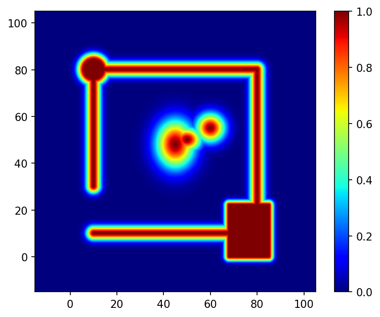
(a) Potential field

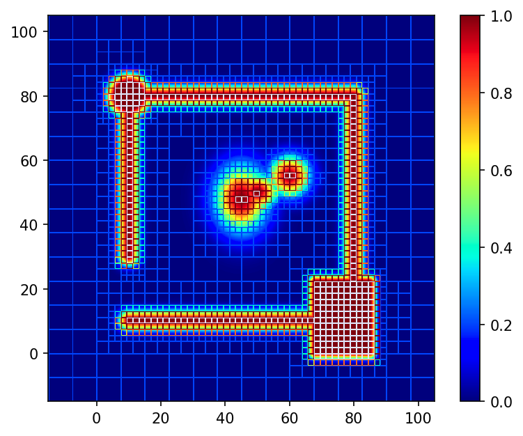
(b) Quad cells

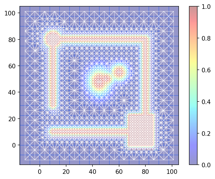
(c) Routing network

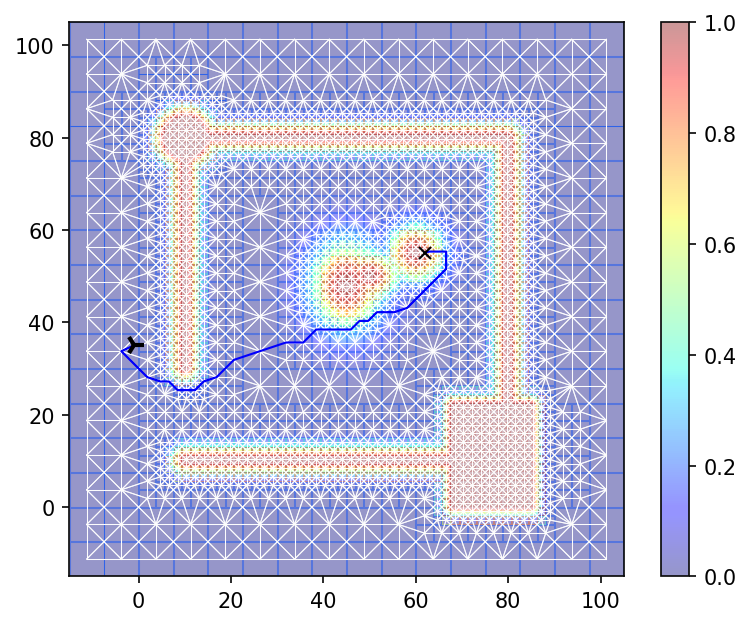
(d) A route in the network

Figure 1: Stages of Larp for a walled room scene

III-A Multi-Scale Cell Decomposition

Drawing inspiration from adaptive quad tree cell decomposition, the first phase consists of partitioning a potential field into a multitude of cells, each varying in size. These cells are then correlated with their respective potential for infringing upon nearby restrictions. The stratagem for cell subdivision is calibrated, ensuring that cells proximal to obstacles are proportionately smaller, thereby augmenting routing precision and safety. Fig. 1(b) illustrates this decomposition for a walled room scene. The methodology behind cell decomposition is expounded in Algorithms 1 and 2.

Algorithm 1 Larp – Quad Tree Cell Decomposition

minimum cell size $n_{min}$; maximum cell size $n_{max}$

Cells containing restriction have highest potential

function Build($x$, $n$, $U$)

     $quad\leftarrow QuadNode(x,n)$

     $zones\leftarrow$ map with default farthest zone

     if $|U|>0$ then

         $zones\leftarrow$ ApproxDistanceZones($x$, $n$, $U$)

     end if

     $quad.zone\leftarrow\min(zones)$ $\triangleright$ Farthest zone if empty

     if $n\leq n_{max}$ then

         if $n\leq n_{min}$ or $quad.zone$ is farthest zone then

              Mark $quad$ as leaf

              return $quad$

         else if $quad.zone>0$ then

              $\bar{U}\leftarrow\{u\in\,$U$\,|\,zones[u]=quad.zone\}$

              $\bar{C}\leftarrow\{c=x+\frac{n}{\sqrt{2}\,|\bar{x}_{u}(x)|}\,\bar{x}_{u}(x)\,|\,u\in\,\bar{U}\}$

              $bd_{l}\leftarrow boundary\_egde[quad.zone]$

              for each point $c$ in $\bar{C}$ do

                  if given any $u\in\bar{U}$, $\tilde{d}_{u}^{2}(x)<bd_{l}$ then

                       Mark $quad$ as leaf

                       return $quad$

                  end if

              end for

         end if

     end if

     $U\leftarrow\{u\in\,$U$\,|\,zones[u]<$ farthest zone$\}$

     for each quad $q$ of a cell do

         $quad.child[q]\leftarrow$ Build($q.center$, $n/2$, $U$)

     end for

     return $quad$

end function

$root\leftarrow$ BUILD(field.center, field.size, all units in field)

Algorithm 2 Larp – Estimate Boundary of Cell

Sorted list of boundaries $bds$ in ascending order

function ApproxDistanceZones($x$, $n$, $U$)

     $zones\leftarrow$ map with default further zone

     for each unit $u$ in $U$ do

         if $d_{u}^{2}(x)\leq\frac{n^{2}}{2}$ then

              $zones[u]\leftarrow 0$

         end if

     end for

     for each unit $u$ in $U$ but not already in $zones$ do

         $dist=\tilde{d}_{u}^{2}(x)$

         Assign $zones[u]$ into bin given $bds$ and $dist$

     end for

     return $zones$

end function

III-B Routing network

To streamline path planning within the designated space, a network graph is constructed subsequent to the potential field’s decomposition. The process employs a divide-and-conquer approach to traverse the quad tree, facilitating the identification of neighboring nodes for any given leaf quad node. The intricacies of the field are distilled into a simplified network, where each graph node correlate with a leaf cell and its upper bound potential for the vicinity. Fig. 1(c) provides a visual representation of this network graph.

In the interest of brevity, we have omitted the detailed adjacency algorithm used to construct the routing network; however, it is available for review in our public repository.

III-C Path Planning

Upon the establishment of the network, the implementation of any graph routing algorithm that simultaneously minimizes route distance and accumulated potential is feasible. For this study, we employ a modified variant of the renowned A* algorithm, wherein the distance function is redefined as:

$$d(q_{a},q_{b})=s(q_{b})\cdot\|q_{a}.\text{center}-q_{b}.\text{center}\|$$ (1)

where $q_{a}$ and $q_{b}$ denote the quadrant being traversed from and to, respectively; $s(q)$ represents a hyper-parameter scale transformation function that modulates the safety distance; and $q_{a}.\text{center}$ signifies the centroid of cell $q_{a}$. A route generated for the walled room scene is depicted in Fig. 1(d). Subsequent to determining a routing solution, line segments are integrated to connect the initial location and the destination with the discovered route within the network.

III-D Safety Validation

Prior to assessing the safety of a route, it is imperative to define what constitutes a route within a potential field.

Definition 4 (Route in a Potential Field).

A route $R$ within a restrictive routing potential field is delineated as a trajectory comprising a line string that interconnects a sequence of points, expressed as:

$$R_{p}=\{x_{1},x_{2},...,x_{N}\}$$

where $x_{i}$ signifies a 2D coordinate in a plane, and $N-1$ represents the count of consecutive line segments that constitute the line string.

With Definition 4 established, several metrics to evaluate the safety of a route can be examined. The primary metric is the cumulative potential under a route’s trajectory, calculated as:

$$R_{A}=\int_{R}\sigma(x_{t})\,dx_{t}=\sum^{N-1}_{i=0}\int_{x_{i}}^{x_{i+1}}\sigma(x_{t})\,dx_{t}$$ (2)

where $\sigma(\cdot)$ denotes the potential field assessment, and $\int_{x_{i}}^{x_{i+1}}\sigma(x_{t})\,dx_{t}$ encapsulates the line integral from point $x_{i}$ to point $x_{i+1}$. This metric gauges the aggregate potential for committing a restriction violation by an agent traversing the route, with higher values indicating increased interaction with restricted regions.

Conversely, a route’s length as a measure of safety is considered:

$$R_{d}=\int_{R}1\,dx_{t}=\sum^{N-1}_{i=0}\int_{x_{i}}^{x_{i+1}}1\,dx_{t}$$ (3)

The extended duration of a route implies a prolonged presence within the field, potentially elevating the risk of violation occurrences.

Ultimately, combining these two metrics yields a composite measure that reflects the average engagement with restrictions along a route

$$R_{avg}=\frac{R_{A}}{R_{d}}$$ (4)

A heightened $R_{avg}$ value suggests a route’s active proximity to restricted areas. Empirical observations indicate that a threshold of 0.35 or below is typically indicative of minimal engagement with restrictions.

IV Experiments and Results

IV-A Potential field-based path planning algorithms

To assess the efficacy of our algorithm, we have compiled a suite of path planning strategies that leverage potential fields to evaluate proximity to obstacles and violating routing restrictions. Detailed implementations and comparisons of these methods are available in our Github repository at https://github.com/wzjoriv/path-planning-pf.

IV-A1 Penalty Method with Gradient Descent (PM)

The penalty method with gradient descent introduces an attractive force that propels an agent towards a goal, defined as:

$$F_{A}(x)=\zeta(x_{g}-x)$$ (5)

where $\zeta$ is a scalar hyper-parameter dictating the strength of the attraction, and $x_{g}$ denotes the goal’s location. Additionally, a repulsive force emerges from a penalty on the potential field value,

$$F_{R}(x)=-\eta\,p^{\prime}(\sigma(x))\,\nabla\sigma(x)$$ (6)

where $\eta$ is a scalar hyper-parameter governing the repulsion, $p^{\prime}(\cdot)$ is the derivative of the penalty function, and $\nabla\sigma(x)$ represents the gradient of the potential field under discussion.

Combining these two forces forms a traversal strategy that steers the agent towards the goal, articulated as:

$$x_{i+1}=x_{i}+\gamma\,\frac{F_{A}(x_{i})+F_{B}(x_{i})}{\|F_{A}(x_{i})+F_{B}(x_{i})\|}$$ (7)

where $\gamma$ signifies the step size, and $x_{0}$ is the agent’s initial location. To circumvent local minima near the goal, our experiments introduce a heuristic: if $\|x_{N}-x_{g}\|\leq 2.5$, a direct line segment to the goal $x_{g}$ is appended to the route’s $R_{p}$.

IV-A2 Artificial Potential Field (APF, APF(*))

The classical APF method supplants the gradient-based approach with a traditional repulsive force as delineated in [10, 22]. Within the scope of the problems addressed, this repulsive force is articulated by:

$$F_{R}(x)=\begin{cases}\eta\left(\frac{1}{d(x)}-\frac{1}{d_{o}}\right)\frac{1}{d\,^{2}(x)}\bar{x}(x),&\text{if }d(x)\leq d_{o}\\ 0,&\text{otherwise}\end{cases}$$ (8)

where $d(x)=\sqrt{d\,^{2}(x)}$, $d_{o}$ is the threshold distance at which the repulsive force becomes active, and $\bar{x}(x)$ is the repulsion vector from the nearest obstacle.

Subsequent enhancements to the APF methodology, not originally included but recommended for improved efficacy, propose an alternative attraction force [22]:

$$F_{A}(x)=\begin{cases}\zeta(x_{g}-x),&\text{if }\|x-x_{g}\|\leq d_{g}\\ \zeta\,d_{g}\frac{x_{g}-x}{\|x-x_{g}\|},&\text{otherwise}\end{cases}$$ (9)

where $d_{g}$ is the critical distance beyond which the attraction force adopts a quadratic profile to ensure a smooth convergence to the target.

For the APF method, a variant denoted as APF (*) is also implemented for which square distance function $\mathbf{\text{d}}\,^{2}(x)$ is substituted with its scaled counterpart $\tilde{d}\,^{2}(x)$.

IV-A3 Modified Artificial Potential Field (M-APF)

M-APF, an advanced iteration of APF introduced by [8, 23], innovates upon the conventional repulsion force to mitigate the issue of local minima. The reformulated force is expressed by:

$$\begin{split}F_{R1}(x)&=\eta\left(\frac{1}{d(x)}-\frac{1}{d_{o}}\right)\|x-x_{g}\|\,^{m-3}\\ F_{R2}(x)&=\eta\,m\left(\frac{1}{d(x)}-\frac{1}{d_{o}}\right)^{2}\|x-x_{g}\|\,^{m}\\ \\ F_{R}(x)&=\begin{cases}F_{R1}(x)+F_{R2}(x)\frac{\bar{x}(x)}{\|\bar{x}(x)\|},&\text{if }d(x)\leq d_{o}\\ 0,&\text{otherwise}\end{cases}\end{split}$$ (10)

where $m$ is a positive scalar hyper-parameter that modulates the repulsion force’s sensitivity to the agent’s proximity to the goal.

IV-B Results

In evaluating these algorithms, we explored three distinct scenarios of path planning.

IV-B1 Scenario 1 (Unobstructed Path)

The first scenario considers a straightforward path planning task where the objective is to travel towards an unobstructed target. Although there are no significant obstacles present, this scenario serves to accentuate the subtle differences between the algorithms. As shown in Table II and Fig. 2, even in an ideal situation where no obstacles impede the path, Larp—placing a premium on safety—may yield routes that are marginally longer if it results in a lower overall potential energy.

TABLE II: Performance metrics for Scenario 1. All algorithms successfully reach the goal. Larp generates a slightly longer path due to its conservative movements and emphasis on safety. A $\checkmark$ under ’Goal Found’ indicates $\|x_{N}-x_{g}\|^{2}\leq 2.5$ where $x_{N}$ is the final position of a route.

Algorithm	Goal Found	Route Distance	Route Area	Average Potential	Highest Potential
PM	✓	62.04	0.4006	0.0065	0.0619
APF	✓	62.06	0.3863	0.0062	0.0594
APF (*)	✓	62.02	0.4020	0.0065	0.0622
M-APF	✓	62.02	0.4020	0.0065	0.0622
Larp (Our)	✓	62.9181	0.1082	0.0017	0.0084

(a) PM

(b) APF

(c) APF (*)

(d) M-APF

(e) Larp (Our)

Figure 2: Comparison of routes in Scenario 1, featuring an unobstructed path. The red marker indicates the initial location of the agent.

IV-B2 Scenario 2 (Obstructed Path and Near-Obstacle Goal)

This scenario examines the algorithms’ performance when an agent must navigate around an obstacle and when the target is in close proximity to one. The results are presented in Table III and Fig. 3. When obstacles are introduced along the route, both PM and APF struggle to maintain a safe distance from the constraints, resulting in higher peak potential values. PM’s dependence on gradients and penalties hinders its ability to significantly deviate from the obstacle’s path. APF’s higher potential can be attributed to its focus on immediate obstacle proximity rather than the overall potential for obstacle avoidance; however, it also contributes to its shorter route distance. Among all the methods evaluated, Larp consistently produced safer routes, albeit at the expense of increased distance. Nevertheless, Larp’s route lengths remain competitive, particularly when compared to methods such as APF (*) and M-APF.

TABLE III: Performance metrics for Scenario 2. The highest potential energy values for APF (*), M-APF, and Larp reflect the goal’s proximity to obstacles.

Algorithm	Goal Found	Route Distance	Route Area	Average Potential	Highest Potential
PM	✓	79.188	23.1432	0.2923	0.9011
APF	✓	77.2863	23.011	0.2977	0.9220
APF (*)	✓	87.8328	29.3081	0.3337	0.8948
M-APF	✓	80.8579	21.0194	0.26	0.8948
Larp (Our)	✓	83.8675	15.8687	0.1892	0.8948

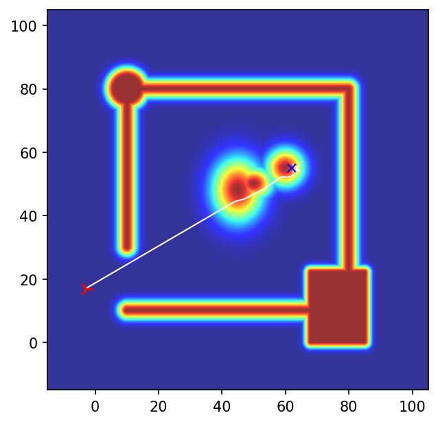
(a) PM

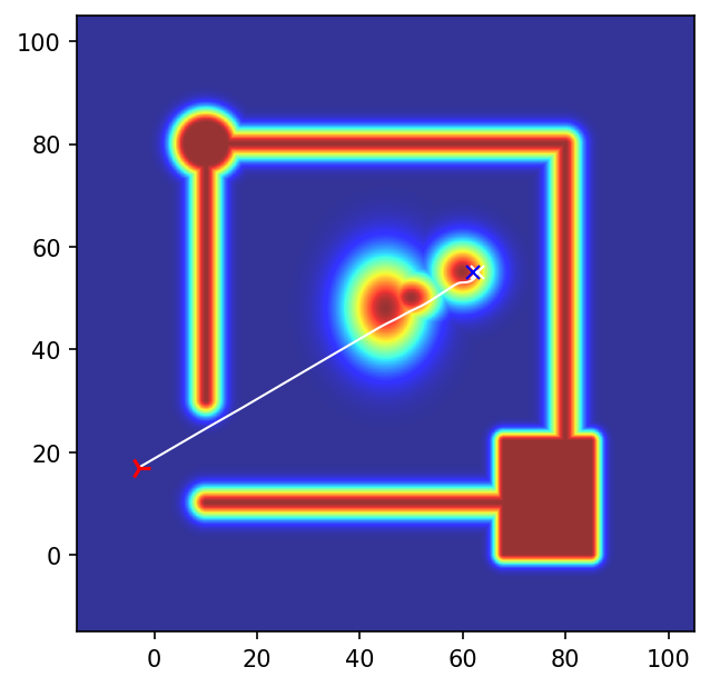
(b) APF

(c) APF (*)

(d) M-APF

(e) Larp (Our)

Figure 3: Scenario 2 of an obstructed path and near-obstacle goal (routes comparison)

IV-B3 Scenario 3 (Walled-Off Path)

The final scenario investigates the behavior of the methods when the direct route to a target is obstructed by a wall. As depicted in Table IV and Fig. 4, all methods, except for Larp, fail to reach the destination. When confronted with non-circular restrictions, both penalty-based and force-based methods may struggle to overcome the local minima created by the opposing forces of attraction and repulsion from the obstacles.

TABLE IV: Performance metrics for Scenario 3. Except for Larp, all other methods are unable to reach the target; therefore, their performance measurements are not valid for comparison but provide insight into their behavior. In this table, an ✗  under ’Goal Found’ indicates $\|x_{N}-x_{g}\|^{2}>2.5$

. Algorithm Goal Found Route Distance Route Area Average Potential Highest Potential PM ✗ 33.32 18.6015 0.5583 0.9529 APF ✗ 42.83 26.3972 0.6163 0.9075 APF (*) ✗ 80.37 53.9457 0.6712 0.8075 M-APF ✗ 38.57 1.8687 0.0485 0.0674 Larp (Our) ✓ 163.8382 14.8769 0.0908 0.3453

(a) PM

(b) APF

(c) APF (*)

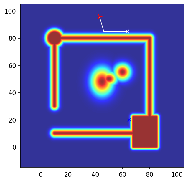
(d) M-APF

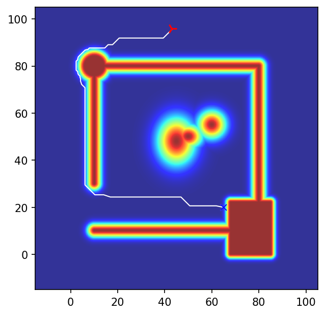
(e) Larp (Our)

Figure 4: Routes comparison for Scenario 3, featuring a walled-off path.

V Conclusion

In this work, we have presented Larp, an innovative path planning framework tailored for restrictive routing within potential fields. Demonstrating superior results, Larp outperforms both traditional and contemporary potential field-based methodologies by reliably crafting safer routes that diminish the risk of restriction violations, all while preserving comparative efficiency in terms of travel distance. This is achieved through an initial segmentation of the potential field into multi-scale cells, with each cell’s restriction zone determined by its proximity to nearby obstacles. For transparency and to facilitate further research, the source code for an official implementation of Larp has been made publicly accessible.

While Larp marks an advancement in route safety, opportunities for improvement remain. The framework’s quad cell decomposition approach and zone classification system are poised for further optimization. The influence of a cell’s dimensions and positioning on the placement of subsequent cells is a critical factor in the pursuit of optimally short and safe routes. Moreover, the current method of zone classification, which relies on an proxy scaled distance to a cell’s periphery to gauge the highest potential across the region, may estimate an higher potential for a region that what it is. Future endeavors will concentrate on refining these elements and developing a dynamic and scalable system capable of storing and updating cells in real-time to adapt to evolving restrictions for unmanned aircraft system traffic management (UTM).

References

- [1] Rakesh Shrestha, Inseon Oh, and Shiho Kim. A survey on operation concept, advancements, and challenging issues of urban air traffic management. Frontiers in Future Transportation, 2:1, 2021.
- [2] Khaled Telli, Okba Kraa, Yassine Himeur, Abdelmalik Ouamane, Mohamed Boumehraz, Shadi Atalla, and Wathiq Mansoor. A comprehensive review of recent research trends on unmanned aerial vehicles (uavs). Systems, 11(8):400, 2023.
- [3] Bhawesh Sah, Rohit Gupta, and Dana Bani-Hani. Analysis of barriers to implement drone logistics. International Journal of Logistics Research and Applications, 24(6):531–550, 2021.
- [4] Josue N Rivera and Dengfeng Sun. Air traffic management for collaborative routing of unmanned aerial vehicles via potential fields, 2024. Submitted to ICRAT 2024.
- [5] Michael Jones, Soufiene Djahel, and Kristopher Welsh. Path-planning for unmanned aerial vehicles with environment complexity considerations: A survey. ACM Computing Surveys, 55(11):1–39, 2023.
- [6] Pengcheng Wu, Junfei Xie, and Jun Chen. Safe path planning for unmanned aerial vehicle under location uncertainty. In 2020 IEEE 16th International Conference on Control & Automation (ICCA), pages 342–347. IEEE, 2020.
- [7] Tai Huang, Kuangang Fan, Wen Sun, Weichao Li, and Haoqi Guo. Potential-field-rrt: A path-planning algorithm for uavs based on potential-field-oriented greedy strategy to extend random tree. Drones, 7(5):331, 2023.
- [8] Seyyed Mohammad Hosseini Rostami, Arun Kumar Sangaiah, Jin Wang, and Xiaozhu Liu. Obstacle avoidance of mobile robots using modified artificial potential field algorithm. EURASIP Journal on Wireless Communications and Networking, 2019(1):1–19, 2019.
- [9] Chunyu Ju, Qinghua Luo, and Xiaozhen Yan. Path planning using an improved a-star algorithm. In 2020 11th International Conference on Prognostics and System Health Management (PHM-2020 Jinan), pages 23–26. IEEE, 2020.
- [10] Yong K Hwang and Narendra Ahuja. A potential field approach to path planning. IEEE transactions on robotics and automation, 8(1):23–32, 1992.
- [11] Jinchao Chen, Mengyuan Li, Zhenyu Yuan, and Qing Gu. An improved a* algorithm for uav path planning problems. In 2020 IEEE 4th Information Technology, Networking, Electronic and Automation Control Conference (ITNEC), volume 1, pages 958–962. IEEE, 2020.
- [12] Jinjun Rao, Chaoyu Xiang, Jinyao Xi, Jinbo Chen, Jingtao Lei, Wojciech Giernacki, and Mei Liu. Path planning for dual uavs cooperative suspension transport based on artificial potential field-a* algorithm. Knowledge-Based Systems, 277:110797, 2023.
- [13] Kaiping Wang, Mingzhu Song, and Meng Li. Cooperative multi-uav conflict avoidance planning in a complex urban environment. Sustainability, 13(12):6807, 2021.
- [14] Mohammadreza Radmanesh, Manish Kumar, Alireza Nemati, and Mohammad Sarim. Dynamic optimal uav trajectory planning in the national airspace system via mixed integer linear programming. Proceedings of the Institution of Mechanical Engineers, Part G: Journal of Aerospace Engineering, 230(9):1668–1682, 2016.
- [15] Yanli Chen, Guiqiang Bai, Yin Zhan, Xinyu Hu, and Jun Liu. Path planning and obstacle avoiding of the usv based on improved aco-apf hybrid algorithm with adaptive early-warning. Ieee Access, 9:40728–40742, 2021.
- [16] Wenbin Hou, Zhihua Xiong, Changsheng Wang, and Howard Chen. Enhanced ant colony algorithm with communication mechanism for mobile robot path planning. Robotics and Autonomous Systems, 148:103949, 2022.
- [17] Chenchen Xu, Xiaohan Liao, Huanyin Yue, Xiaoming Deng, and Xiwang Chen. 3-d path-searching for uavs using geographical spatial information. In IGARSS 2019-2019 IEEE International Geoscience and Remote Sensing Symposium, pages 947–950. IEEE, 2019.
- [18] Jingzhi Hu, Hongliang Zhang, Lingyang Song, Zhu Han, and H Vincent Poor. Reinforcement learning for a cellular internet of uavs: Protocol design, trajectory control, and resource management. IEEE Wireless Communications, 27(1):116–123, 2020.
- [19] Sarthak Bhagat and PB Sujit. Uav target tracking in urban environments using deep reinforcement learning. In 2020 International conference on unmanned aircraft systems (ICUAS), pages 694–701. IEEE, 2020.
- [20] Fuchen Kong, Qi Wang, Shang Gao, and Hualong Yu. B-apfdqn: A uav path planning algorithm based on deep q-network and artificial potential field. IEEE Access, 2023.
- [21] Ahmed S Abdel-Rahman, Shady Zahran, Basem E Elnaghi, and SF Nafea. Enhanced hybrid path planning algorithm based on apf and a-star. The International Archives of the Photogrammetry, Remote Sensing and Spatial Information Sciences, 48:867–873, 2023.
- [22] Howie Choset, Ji Y Lee, G.D. Hager, and Z. Dodds. Lecture notes in robotic motion planning: potential functions, 2010.
- [23] Farid Bounini, Denis Gingras, Herve Pollart, and Dominique Gruyer. Modified artificial potential field method for online path planning applications. In 2017 IEEE Intelligent Vehicles Symposium (IV), pages 180–185. IEEE, 2017.