Early Enrichment Population Theory at High Redshift

Abstract

An Early Enrichment Population (EEP) has been theorized to produce the observed metallicity in the intracluster medium (ICM) of galaxy clusters. This population likely existed at high redshifts (z$\sim$10), relics of which we posit exist today as dwarf galaxies. Previous work argues that the initial mass function (IMF) of the EEP must be flatter than those found at lower redshifts, but with considerable uncertainties. In this work, we present a more quantitative model for the EEP and demonstrate how observational constraints can be applied to the IMF using supernova Type Ia (SNIa) rates, delay time distribution (DTD), and the luminosity function (LF) of galaxy clusters. We determine best-fit values for the slope and mass break of the IMF by comparing IMFs from literature with observed DTDs and the low-luminosity component ($M(R)<-12$) of the Coma LF. We derive two best-fit IMFs: (1) $\alpha_{lo}=-0.13\pm 0.24$ for $0.07<M/M_{\odot}<1.75$ and $\alpha_{hi}=0.53\pm 0.01$ for $1.75<M/M_{\odot}<150$, and (2) $\alpha_{lo}=1.06\pm 0.11$ for $0.07<M/M_{\odot}<6$ and $\alpha_{hi}=0.53\pm 0.01$ for $6<M/M_{\odot}<150$. We also compare these with sl-5 from Loewenstein (2013) with $\alpha=0.5$ for $0.07<M/M_{\odot}<8$ and $\alpha=0.3$ for $8<M/M_{\odot}<150$. This EEP model, along with stars formed at later times, can produce the observed metallicity, is consistent with other observations, and predicts a significant rise in the SNIa rate at increasing redshift.

1 Introduction

Galaxy clusters are the largest gravitationally bound structures in the Universe. Their deep gravitational potential wells allows us to approximate the largest clusters ($10^{13.5}-10^{15}M_{\odot}$) as closed-box systems - all elements produced within the cluster remains there. This makes the hot, X-ray emitting halo the perfect place to study the elemental history of galaxy groups and clusters. The X-ray halo lies within the virial radius of the galaxy cluster and is seen in the energy range $\sim$0.5-12.0 keV - the Intracluster Medium (ICM).

Many have studied the gas phase metallicity of clusters (e.g., Baldi et al., 2012; Mantz et al., 2017; Ghizzardi et al., 2020; Lovisari et al., 2020) and find a universal metallicity $\sim$0.35 $Z_{\odot}$ outside 0.1$R_{500}$ using Asplund et al. (2009) abundances (De Grandi et al., 2004; Mantz et al., 2017; Urban et al., 2017). The ICM metallicity ($Z_{ICM}$) seems to be independent of galaxy cluster mass, or stellar fraction ($M_{*}/M_{gas}$), even over a large range of $M_{*}/M_{gas}$ (0.035-0.43) (Bregman et al., 2010; Blackwell et al., 2022). This is especially confounding when the measured halo metallicity is compared to expectations. A relationship for predicting the halo metallicity from the visible stellar populations ($Z_{*}$) was developed in Loewenstein (2013) as $Z_{*}=1.55(M_{*}/M_{gas})$. For a cluster with $M_{*}/M_{gas}=0.05$, the expected halo metallicty is 0.08$Z_{\odot}$, a factor of $>$4 below $Z_{ICM}$. That is, the visible galaxies and stars in a galaxy cluster cannot have produced the measured ICM metallicity. This discrepancy is the missing metal conundrum and has been discovered and discussed previously (e.g. Elbaz et al., 1995; Mushotzky et al., 1996; Portinari et al., 2004; Renzini & Andreon, 2014; Werner & Mernier, 2020).

Various potential explanations for the missing metal conundrum have been explored with fault found in each. One solution proposes the presence of stars in the ICM which generated sufficient quantities of metals to account for the observed metallicity in high-mass clusters (Renzini & Andreon, 2014). Sivanandam et al. (2009) calculated that intracluster stars with a standard initial mass function (IMF) contribute approximately 25% of the total ICM metallicity within $R_{500}$, but only 20% of the total intracluster light (ICL) (Zibetti et al., 2005; Krick & Bernstein, 2007; Giallongo et al., 2014; Furnell et al., 2021). If these intracluster stars were to supply the missing metals, we would expect to observe a population of intracluster stars at least four times larger than what is detected. A population four times larger, sufficient to explain the absence of metals, would generate at least 80% of the total cluster light, exceeding observations.

Another theory examines the relationship between the IMF of star-forming clouds at redshift $z\sim 2$ and cluster final mass (Renzini & Andreon, 2014). High-mass clusters require an additional source of metals that cannot be accounted for by visible stellar populations. These metals might originate from star-forming clouds at high redshifts prior to the formation of galaxy clusters. High-mass clusters require a larger supply of metals from star-forming clouds compared to low-mass systems (Renzini & Andreon, 2014; Blackwell et al., 2022). In order to compensate for the missing metals, the IMF of star-forming clouds at high redshifts would need to produce more high-mass stars for higher final mass systems and fewer high-mass stars for lower final mass systems. This scenario assumed the star-forming clouds “know” the final cluster mass, which is improbable.

We are left with one theory to consider, a population of stars that existed at high redshifts and supplied high-mass clusters with the missing metals - the early enrichment population (EEP) (Elbaz et al., 1995; Loewenstein, 2001). This theory has emerged from investigations of the evolution of halo metallicity across redshift (Mantz et al., 2017; Flores et al., 2021), and supported by studies of metallicity in relation to the system stellar fraction (Bregman et al., 2010; Blackwell et al., 2022). According to this theory, the EEP would have existed during high redshifts, primarily consisting of early Population II stars. These stars would have played a significant role during the reionization period in protoclusters, $6<z<10$, and would have favored a bottom-light IMF (Fan et al., 2006; Loewenstein, 2013; Planck Collaboration et al., 2016). The EEP would have been present in nascent galaxies, not prominent as $L^{*}$ galaxies, and would not be observable today (Werner & Mernier, 2020).

Currently very little is known about this theory. Few authors have provided calculations of predictions for the contribution of the EEP (Loewenstein 2013, hereafter L13). Recently Blackwell et al. (2022) made calculations of observable and testable quantities for the EEP such as the expected Type Ia supernovae rate. In this paper we examine further aspects about the current state of the EEP theory (Section 2), and provide calculations of predictable and measurable quantities to test this theory such as supernova Type Ia (SNIa) observations (Section 6) and Luminosity Functions (LF, Section 7). These calculations are built off predictions of $Z_{EEP}$, Section 3. The assumptions required to make these calculations and are discussed in Section 4 and Section 5.

2 The Early Enrichment Population

The idea of early chemical enrichment has been discussed for the past three decades (e.g., Renzini et al., 1993; Elbaz et al., 1995; Mushotzky et al., 1996; Loewenstein, 2001; Matteucci & Calura, 2005; Million et al., 2011; Mantz et al., 2017; Blackwell et al., 2022; Sarkar et al., 2022), since the first X-ray spectra of galaxy clusters were studied with an exceptionally prominent Iron (Fe) emission line (e.g., Gursky et al., 1971; Mitchell et al., 1976; Mushotzky et al., 1978). There are small variations, but the general idea between all theories is consistent - the excess abundance of metals in the ICM of high-mass clusters and a seemingly Universal metallicity among galaxy groups and clusters ($\sim$0.35$Z_{\odot}$) is not well explained by standard galaxy cluster enrichment theories. Galaxies within a rich cluster do not have a large enough stellar population to have enriched the ICM to the measured abundance using a fixed IMF. A universal metallicity suggests that an earlier, and external source of metals must exist.

The early enrichment population (EEP) is a theorized population of stars that created most of the metals in high-mass galaxy clusters, and smaller contributions in low-mass galaxy clusters, measured in the ICM today. This population would be primarily early Pop II and late Pop III stars. The exact IMF for Pop III stars remains uncertain; however, it is anticipated to be dominated by medium and high-mass stars ($10-10^{3}M_{\odot}$) (Chantavat et al., 2023, and references therein). Supernovae resulting from the core collapse (SNCC) of high-mass stars primarily yields alpha elements (i.e., carbon, oxygen, nitrogen, magnesium and silicon) and a subset of metal group elements. Pair instability supernovae can occur in stars with masses $\sim$100-260 $M_{\odot}$ but the amount of Fe they produce is negligible, even if they are relatively common (Thielemann et al., 1986, 1996; Ferreras & Silk, 2002; Heger & Woosley, 2005; Woosley & Heger, 2015). The majority of Fe observed in galaxy clusters is generated by SNIa with a typical yield of 0.743 $M_{\odot}$ per Ia and 0.0824 $M_{\odot}$ per CC (Kobayashi et al., 2006; Loewenstein, 2013).

Once Pop III stars pollute their surroundings to a metallicity level exceeding $10^{-6}-10^{-3.5}$ $Z_{\odot}$, the cooling process is primarily governed by fine structure lines (Bromm & Loeb, 2003; Fang & Cen, 2004; Bromm, 2013; Pallottini et al., 2014; Yang et al., 2015; Liu & Bromm, 2020; Corazza et al., 2022). The IMF is then believed to adopt forms similar to those observed during the standard low-redshift regime, marking the transition to the Pop II phase. The Pop II phase overlaps with Pop III but swiftly surpasses it in terms of significance for metal or photoionization production at redshifts z$\sim$11-13 (Yang et al., 2015; Corazza et al., 2022).

Before reionization, the gas remains in a neutral state, enabling easier collapse into stars, particularly dwarf galaxies - dwarf elliptical (dE) galaxies in clusters, a likely host for the EEP. At $z\sim 10$ the $T_{CMB}\sim 30$ K which raises the Jeans mass and potentially modifies the low-mass segment of the IMF. During the reionization period ranging $6<z<9$, it is expected that Pop II stars dominate (Fan et al., 2006; Planck Collaboration et al., 2016; Jaacks et al., 2019). For these reasons, we believe the EEP primarily occurs before reionization reaches completion and is dominated by a bottom-light and/or top-heavy IMF. Few works have investigated the exact shape of the EEP IMF, narrowing possibilities simply on the abundances required (Loewenstein, 2013; Corazza et al., 2022).

Initial studies of the EEP contribution to galaxy groups and clusters suggests that the EEP may have began at different epochs (z=12 vs z=7) (Corazza et al., 2022). Systems with the same value of $M_{*}/M_{gas}$, similar halo masses, and implied EEP metallicity contribution ($Z_{EEP}$) have varying $Z_{ICM}$ around the mean (discussed further in Section 3). This implies differences in the efficiency of the EEP in different galaxy clusters which may be a result of some systems having longer periods of star formation with a flatter IMF.

Two further constraints on the EEP IMF are the observed SNIa and the remaining light from the EEP. A more recent time of formation would result in a higher number of observed SNIa at more recent times. With a time formation at $z\sim 10$, stars with mass $<$1$M_{\odot}$ would still exist today. If the EEP formed pre-reionization, we would expect to see these stars in the dwarf Elliptical (dE) galaxies in groups and clusters. Thus, the number of SNIa and total luminosity of dE galaxies (the theorized hosts of the EEP) within a cluster places a constraint on the high and low-mass end of the EEP IMF respectively, and the time of formation.

3 $Z_{ICM}$ versus $M_{*}/M_{gas}$ Survey

The main objective of this survey was to perform a comprehensive and uniform analysis of a large data set over a range of 0.035-0.43 $M_{*}/M_{gas}$ (Table 1). We obtained values of $M_{*,500}$ and $M_{gas,500}$ for 25 systems from a single source to gain deeper insights into the relationship between $Z_{ICM}$ and $M_{*}/M_{gas}$ (Laganá et al., 2013). Each system was identified to have sufficient counts ($>$40,000 within $R_{500}$) of archival XMM Newton data to derive the average ICM metallicity ($Z_{ICM}$) with an error margin of approximately 10%. All systems have an angular size less than the XMM Newton EPIC camera allowing an on-chip background to be used. Additional systems were reported in Laganá et al. (2013) with suitable $M_{*,500}$ and $M_{gas,500}$ and sufficient archival data, however the systems were not relaxed and therefore not suitable for this survey (i.e., A115 Gutierrez & Krawczynski 2005; Hallman et al. 2018).

Table 1: Summary of galaxy group and cluster $Z_{ICM}$ survey. Values of $M_{*}$ and $M_{gas}$ within $R_{500}$ were obtained from Laganá et al. (2013).

Cluster	RA&DEC	$M_{*}/M_{gas}$	$Z_{ICM}$ (solar)
A2069	15:24:39.8+29:53:26.3	0.035$\pm$0.009	0.44$\pm$0.04
A697	08:42:57.6+36:21:55.8	0.044$\pm$0.013	0.34$\pm$0.04
A665	08:30:57.36+65:50:33.36	0.046$\pm$0.014	0.43$\pm$0.09
MS1455.0+2232	14:57:15.12+22:20:35.52	0.066$\pm$0.020	0.49$\pm$0.03
A1763	13:35:18.24+40:59:59.28	0.069$\pm$0.021	0.40$\pm$0.05
A1914	14:26:99.96+37:39:33.96	0.069$\pm$0.021	0.40$\pm$0.040
A2409	22:00:52.8+20:58:27.84	0.073$\pm$0.022	0.47$\pm$0.03
RXJ1720+2638	17:20:16.8+26:38:06.6	0.077$\pm$0.024	0.56$\pm$0.03
A773	09:17:53.04+51:43:39.72	0.083$\pm$0.025	0.38$\pm$0.05
A1413	11:55:18+23:24:17.28	0.088$\pm$0.026	0.44$\pm$0.01
A781	09:20:26.16+30:30:02.52	0.091$\pm$0.028	0.31$\pm$0.05
A2261	17:22:27.12+32:07:56.28	0.095$\pm$0.029	0.44$\pm$0.04
A1689	13:11:29.52-01:20:29.68	0.098$\pm$0.029	0.38$\pm$0.02
A267	01:52:42.14+01:11:41.29	0.106$\pm$0.032	0.45$\pm$0.06
AWM4	16:04:57+23:55:14	0.111$\pm$0.026	0.49$\pm$0.03
A383	02:48:03.43-03:31:45.87	0.123$\pm$0.038	0.49$\pm$0.04
A1991	14:54:30.2+18:37:51	0.163$\pm$0.045	0.50$\pm$0.04
NGC4325	12:23:06.7+10:37:16	0.193$\pm$0.054	0.36$\pm$0.02
MS0906.5+1110	09:09:12.72+10:58:32.88	0.209$\pm$0.071	0.48$\pm$0.07
A2034	15:10:12.48+33:30:28.08	0.234$\pm$0.069	0.37$\pm$0.05
A2259	17:20:10.08+27:39:03.28	0.273$\pm$0.084	0.40$\pm$0.03
NGC4104	12:06:39+28:10:27	0.337$\pm$0.089	0.45$\pm$0.06
RXCJ2315.7-0222	23:15:44.1-02:22:59	0.376$\pm$0.011	0.41$\pm$0.02
A586	07:32:20.16+31:37:55.92	0.430$\pm$0.134	0.40$\pm$0.03
NGC1132	02:52:51.9-01:16:29	0.484$\pm$0.098	0.31$\pm$0.01

We followed the data reduction and analyses methods outlined in Blackwell et al. (2022). We used CIAO (version 4.12) for all data reduction, and the most recent calibration files, CALDB (version 4.9.3). To analyze the ICM metallicity in these systems, we divided each into five radial bins centered on the X-ray center. The radial bins were defined as: $<0.15$ $R_{500}$, $0.15-0.3$ $R_{500}$, $0.3-0.55$ $R_{500}$, $0.55-0.75$ $R_{500}$ and $0.75-1$ $R_{500}$. During spectral extraction and fitting we took the point spread function into account by generating crossarfs. These redistribute the X-ray photons into the respective annuli where they physically originated but may not be detected. Additionally, we extracted two spectra from the PN chip to improve counting statistics using PATTERN=0 and PATTERN=4 for a low and high-energy spectrum, respectively. We excluded the central annulus when calculating $Z_{ICM}$ and took a weighted average of the fit-determined metallicites from all other annuli. Presentation of results of each cluster will be given in an upcoming paper.

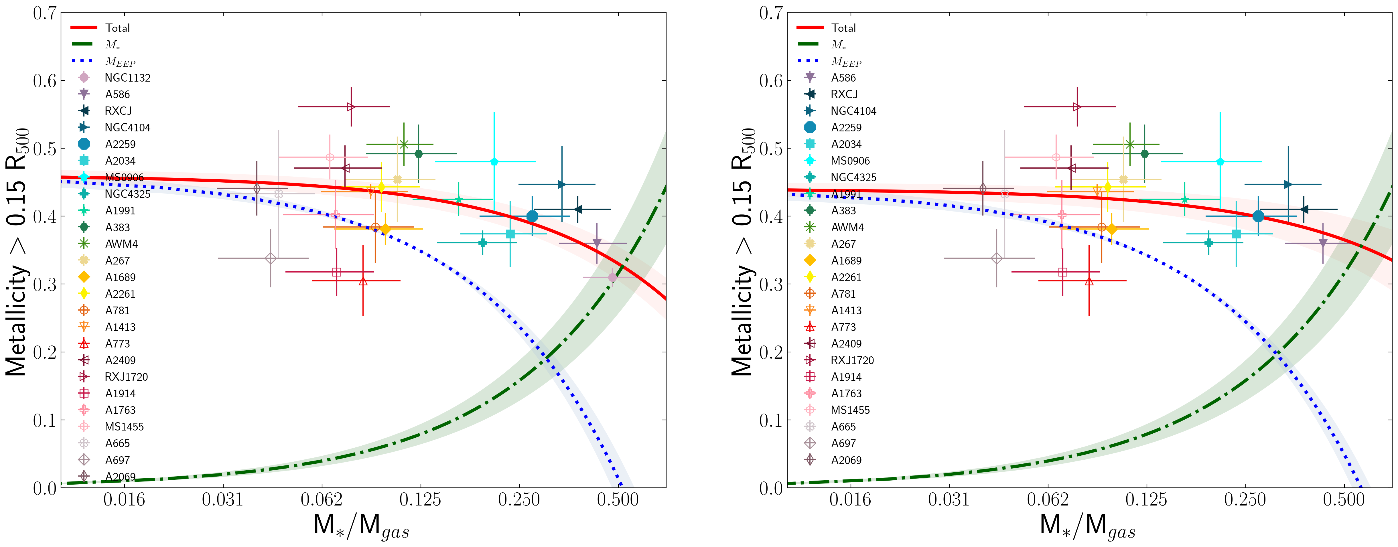
Figure 1: Left: ICM metallicity measurements for 25 galaxy groups and clusters outside of the core of the cluster (defined as $0.15R_{500}$) versus the stellar fraction, $M_{*}/M_{gas}$, of the system. The red solid line shown the total fit of $Z_{ICM}=(-0.26\pm 0.03)\times(M_{*}/M_{gas})+(0.46\pm 0.01)$, done in linear-space. The x-axis is presented in log-scale. The green dash-dot line is the contribution from the stellar population, modeled as $Z_{*}=(0.63\pm 0.12)(M_{*}/M_{gas})$. The trend for $Z_{*}$ is subtracted from the total fit to find $Z_{EEP}=(-0.89\pm 0.12)(M_{*}/M_{gas})+(0.46\pm 0.01)$, shown in the dotted blue line. Shaded regions around each line show the 1$\sigma$ confidence range. Right: The same as the left figure, but excluding NGC1132. This results in $Z_{ICM}=(-0.15\pm 0.05)(M_{*}/M_{gas})+(0.44\pm 0.01)$, and $Z_{EEP}=(-0.78\pm 0.13)(M_{*}/M_{gas})+(0.44\pm 0.01)$. This is the trend adopted for future calculations and is valid over $0.035<M_{*}/M_{gas}<0.43$.

The results of this survey are shown in Figure 1 as a plot of $Z_{ICM}$ versus $M_{*}/M_{gas}$, and Table 1. The overall fit to the trend was done using linear regression and found to be $Z_{ICM}=(-0.26\pm 0.03)(M_{*}/M_{gas})+(0.46\pm 0.01)$ (left plot of Figure 1). This fit indicates a minor dependence of $Z_{ICM}$ on $M_{*}/M_{gas}$, however we note the slope is driven by the data points at high $M_{*}/M_{gas}$. There are only 7 data points with $M_{*}/M_{gas}>0.20$. It is likely that this negative trend is not physical, but rather a result of incompleteness of the sample at high $M_{*}/M_{gas}$. Galaxy cluster NGC1132 has the highest stellar fraction ($0.48\pm 0.09$) with $Z_{ICM}=0.31\pm 0.01$. Excluding this point from our fitting alters $Z_{ICM}=(-0.15\pm 0.05)(M_{*}/M_{gas})+(0.44\pm 0.01)$. We performed Jackknife resampling to ensure that the slope remained constant within $1\sigma$ after removing subsequent highest $M_{*}/M_{gas}$ systems. The fit slope remains constant within $1\sigma$ after NGC1132 and subsequent systems are removed, thus we adopt the most recent fit for $Z_{ICM}$ (right plot of Figure 1).

We also note the dispersion of systems, the largest of which occurring at low $M_{*}/M_{gas}$. We can make a rough estimate of the contribution of the intrinsic variation to the total scatter. The total scatter may be written as $\sigma=\sqrt{\sigma_{met}^{2}+\sigma_{int}^{2}}$, where $\sigma_{met}$ is the average error on $Z_{ICM}$ and $\sigma_{int}$ is the inferred intrinsic scatter. The average error of $Z_{ICM}$ is 0.039 $Z_{\odot}$, and $\sigma$=0.052 $Z_{\odot}$ over all stellar fractions. Solving for $\sigma_{int}$, we find 0.034. Approximately half of the scatter around the expected $Z_{ICM}$ is intrinsic.

The value of $Z_{ICM}$ is the sum of the metals produced by the stars in the system, $Z_{*}$, and the contribution from the EEP, $Z_{EEP}$. Both $Z_{*}$ and $Z_{EEP}$ may be written as their own functions of the stellar fractions of their relative stellar populations multiplied by a constant as seen in Equation 1.

$$Z_{ICM}=Z_{*}+Z_{EEP}=a_{1}(M_{*}/M_{gas})+a_{2}(M_{EEP}/M_{gas})$$ (1)

Loewenstein (2013) developed a relationship for $Z_{*}$ as a function of $M_{*}/M_{gas}$, specifically for Fe return, $Z_{*}=1.55(M_{*}/M_{gas})$. This was determining by considering the metals locked up in stars, mixing of metals with the ICM, and efficiency of star formation. However, this derived trend of $Z_{*}$ over predicts the amount of metals produced in high $M_{*}/M_{gas}$ systems. This drives the derived value of $Z_{EEP}$ to nonphysical negative values. For this reason, we recalculate the expected contribution from $Z_{*}$. We assume two values are known: (1) no metals will be produced for a system with $M_{*}/M_{gas}=0$, (2) the highest stellar fraction system (NGC1132 with $M_{*}/M_{gas}=0.48\pm 0.09$) has $Z_{*}=Z_{ICM}$ (L13). From this we derive $Z_{*}=(0.63\pm 0.12)(M_{*}/M_{gas})$.

The value of $Z_{EEP}$ may be found from subtracting $Z_{*}$ from $Z_{ICM}$ resulting in $Z_{EEP}=(-0.78\pm 0.13)(M_{*}/M_{gas})+(0.44\pm 0.01)$ valid over the range of $0.035<M_{*}/M_{gas}<0.43$. It is this derived trend of $Z_{EEP}$ that we base further calculations on as we are able to calculate the contribution of the EEP population to each system.

We intend to further explore the relationship between $Z_{ICM}$, $Z_{*}$, $M_{*}/M_{gas}$, and other properties of galaxy groups and clusters in a future work.

4 Assumptions

In order to move forward with calculations about the EEP, we must make assumptions about key quantities. We discuss the major assumptions made in the following list:

• We adopt a $\Lambda$CDM cosmology with $H_{0}=70$ km s^-1 Mpc^-1, a baryon density parameter of $\Omega_{b}=0.046$, dark matter density parameter of $\Omega_{DM}=0.24$, and the total baryon density parameter is $\Omega_{m}=0.29$.

• The relative Fe mass yields for SNIa and SNcc adopted are $y_{Ia}=0.734M_{\odot}$ and $y_{CC}=0.0825M_{\odot}$. These values follow from L13 and Kobayashi et al. (2006).

• We adopt an expected $Z_{ICM}$ stellar contribution as $Z_{*}=(0.63\pm 0.12)(M_{*}/M_{gas})$ as derived in Section 3.

• We adopt four IMFs (Figure 3) to proceed with calculations, discussed further in Section 5. Each IMF chosen has been shown to reproduce $Z_{ICM}$ (Loewenstein, 2013; Corazza et al., 2022).

• We adopt a progenitor mass range for SNIa of 3-8 $M_{\odot}$ and SNCC of 8-95 $M_{\odot}$. Both L13 and Maoz & Mannucci (2012) assumed a mass range of 3-8 $M_{\odot}$ for SNIa progenitors. However, recent modeling of Type Ia systems suggests that the lower limit could be $\sim$1.8$M_{\odot}$ (e.g. Antoniadis et al., 2020). With the IMFs adopted, the percentage of stars within the 2-3 $M_{\odot}$ range from 1.36%-12.28%. We proceed with a conservative approach and adopt a lower mass limit of 3 $M_{\odot}$, potentially underestimating the number of expected SNIa. For further discussion and recent on SNIa progenitors, we point the reader to Liu et al. (2023). The upper limit for CC requires consideration of the low-mass cutoff for pair-instability supernovae (PISN), which is 65-140 $M_{\odot}$ (Heger & Woosley, 2002; Chatzopoulos & Wheeler, 2012; Morsony et al., 2014). From Woosley (2017), a star with initial mass 95 $M_{\odot}$ will result in a PISN producing 0.0045 $M_{\odot}$ of Fe. The mass range 95-150 $M_{\odot}$ comprises $3.5\%$ of a diet-Salpeter IMF, contributing only $0.6\%$ of the total Fe to $Z_{ICM}$, a negligible amount. We choose 95 $M_{\odot}$ to be conservative within the uncertainty of CC versus PISN cutoff while accounting for a majority of the stellar population and Fe production.

5 Initial Mass Function

The current initial mass function (IMF) of the EEP is unknown, yet a few constraints are available (described figuratively in Figure 2). The IMF must be bottom-light with a higher low-mass cutoff in order to produce the amount of metals measured in the ICM today without being visible. The formation time period must also align with observations of SNIa as the total number of SNIa would exceed observations if the stellar formation is too close to present day.

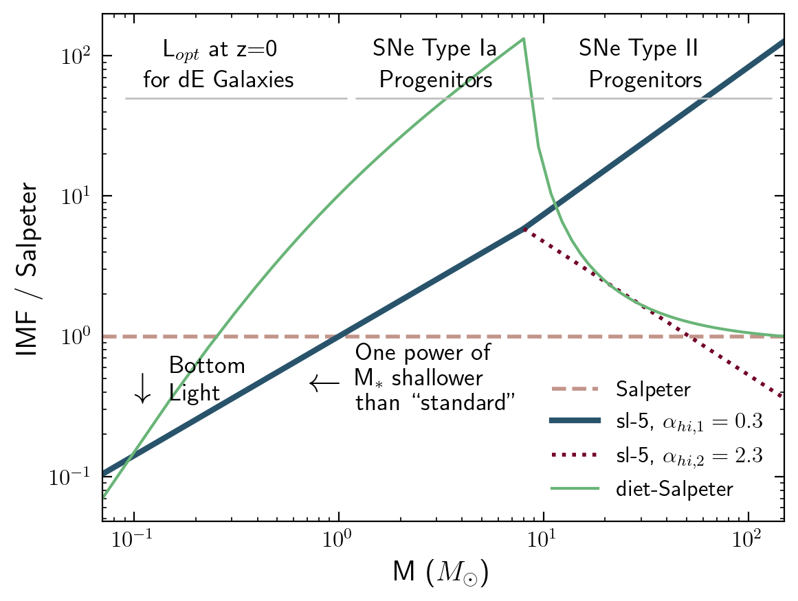
Figure 2: Schematic showing different mass ranges of the IMF that may be constrained through various measurements. The IMFs shown are sl-5 from L13 (solid blue and dotted purple lines), and the diet-Salpeter (as adopted in Blackwell et al. (2022)), divided by Salpeter (dashed light purple line). The IMFs are described in Table 2.

Possible IMFs for the EEP population have been discussed in L13 and Corazza et al. (2022). However, all constraints were placed with the goal of recreating the measured metal abundance only. Here we include other observational constraints such as the SNIa rate as a function of redshift and the observed luminosity function of galaxy groups and clusters to better constraint the EEP IMF and time of formation. SNIa produce a significant amount of iron, so they dominate the metal production of the EEP. Enough high-mass stars must be formed to produce SNIa, but the total number of SNIa required to produce $Z_{EEP}$ must not exceed the rate observed in galaxy groups and clusters. If the EEP formed pre-reionization, we expect dE galaxies to be the primary hosts of the EEP. The luminosity of the remaining low mass ($<$1$M_{\odot}$) stars must not exceed the luminosity of dE galaxies observed in LFs.

There are three observational constrains for the IMF of the EEP: (1) the Fe mass of the EEP, (2) the SNIa rate, (3) the luminosity function (LF) of dEs (remnants of the EEP). We assume various IMFs (Table 2) to make calculations with in order to determine the expected measurable quantities (SNIa rate and dE LFs) which can then be compared to observations. There are a total of 14 IMFs developed in L13 and Corazza et al. (2022) from which we pick 4, shown in Figure 3. These IMFs were chosen as they span the full range of possible IMFs that produce $Z_{ICM}$. IMFs sl-1 and sl-5 have the lowest and highest (respectfully) possible mass breaks and powerlaw-slope values (L13), ultimately containing all values of possible IMFs. The diet-Salpeter IMF was chosen as a continuation from Blackwell et al. (2022), and that from Corazza et al. (2022) is the only determined from simulations and is the highest powerlaw-slope. All IMFs take the functional form $\Phi(m)=m^{-(1+\alpha)}$. We show the four IMFs that are to be adopted for further calculations as well as some more well-known IMFs, such as the Kroupa (Kroupa, 2001), in Figure 3.

Name	$\alpha$	Mass Range ($M_{\odot}$)	Reference
diet-Salpeter	0.35	0.5-1	Blackwell et al. (2022)
	1.35	1-150
C22	1.85	0.1-100	Corazza et al. (2022)
sl-1	-0.7-1.4	0.07-1	L13
	1.3	1-150
sl-5	0.5	0.07 - 8	L13
	0.3-2.3	8-150
Kroupa	1.3	0.08-0.5	Kroupa (2001)
	2.3	0.5-150

Table 2: Initial mass functions adopted for further calculations. Each IMF has been shown to properly recreate the measured ICM abundance, $Z_{ICM}$. Kroupa is included for comparison.

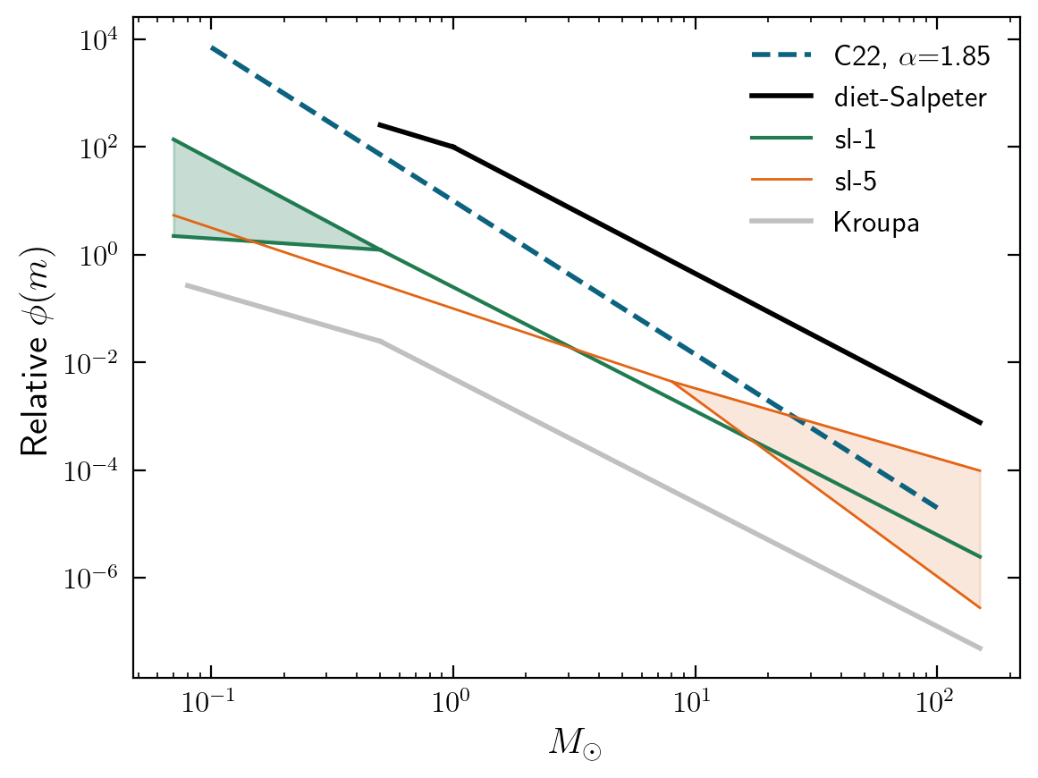
Figure 3: Adopted IMFs for calculations shown compared to a Kroupa IMF (grey line). The normalization of the IMFs have been offset for better visualization. The shaded green and orange regions show the variations in the IMF slope allowed for those mass ranges and derived IMFs from L13.

6 Type Ia Supernovae

Supernovae Type Ia (SNIa) can be seen long after the formation of the initial stellar population. The number and distribution of SNIa observed is heavily influenced by the period and shape of star formation and the number of stars within the progenitor mass range of SNIa formed ($3-8M_{\odot}$). The later is entirely dictated by the IMF of the initial stellar population. That is, the number and distribution of SNIa observed can be used to constrain the IMF. If the IMF slope within the mass range $3-8M_{\odot}$ is more shallow, more SNIa will be produced and subsequently observed compared to an IMF with a steeper slope within the same mass range. In this section we discuss the current constrains of the IMF using the observed distribution of SNIa over cosmic time within galaxy clusters.

6.1 Delay Time Distribution

The number of supernovae Type Ia (SNIa) as a function of redshift since formation can be described by the delay time distribution (DTD) over the redshift range $\sim$10-0 (Gal-Yam & Maoz, 2004). The DTD, Equation 2, has been characterized in galaxy groups and clusters beginning with a starburst assumption and nearby systems then evolving to include various star formation scenarios and observations of SNIa rates in systems out to $z=1.75$ (e.g. Maoz et al., 2010; Freundlich & Maoz, 2021).

$$DTD(t)=R_{1}\big{(}\frac{t}{Gyr}\big{)}^{\alpha}$$ (2)

More recently, the constraint on the star formation history has been relaxed to extended star formation histories deriving an amplitude of $R_{1}=0.41^{+0.12}_{-0.10}\times 10^{-12}$ yr^-1 M${}_{\odot}^{-1}$ and a power-law index $\alpha=-1.09^{+0.15}_{-0.12}$ (Freundlich & Maoz, 2021).

We use this DTD derivation to recreate the expected DTD for the EEP of a single system by first calculating the number of required SNIa to form $Z_{EEP}$, then normalizing the integrated DTD to the total number of EEP SNIa as done in Blackwell et al. (2022). We choose galaxy cluster A2261 for this analysis as it has a stellar fraction of $0.095\pm 0.029$, and fit ICM metallicity= $0.44\pm 0.04$ $Z_{\odot}$, that fall in the middle of the survey systems. We determine the contribution of the EEP to the total ICM metallicity of A2261 using $Z_{*}=(0.63\pm 0.12)(M_{*}/M_{gas})$ and subtracting this from the $Z_{ICM}=0.44\pm 0.03$ $Z_{\odot}$, as described in Section 3. Thus, we find $Z_{EEP}=0.38\pm 0.04$ $Z_{\odot}$. We then multiply $Z_{EEP}$ by the baryonic mass of A2261, $M_{bary}=1.06(\pm 0.034)\times 10^{14}$ $M_{\odot}$, and fractional value of Fe in the sun ($Z_{\odot}^{Fe}=$0.0018) to find the resulting Fe mass from the EEP $M_{Fe,EEP}=7.7(\pm 0.8)\times 10^{10}$ $M_{\odot}$(Grevesse & Sauval, 1999; Asplund et al., 2009; Lodders, 2021).

The total number of SNe (Type Ia + CC) is found by dividing $M_{Fe,EEP}$ by the average Fe yield from the SNe, Equation 3. The relative SNe yields are assumed values of $y_{Ia}=0.743M_{\odot}$ and $y_{CC}=0.0825M_{\odot}$ (Kobayashi et al., 2006). However, the fractional occurrences of each SNe ($f_{ia}$ and $f_{CC}$) are dependent on the type of IMF assumed and can be determined by integrating the IMF over a predefined progenitor mass range for each pathway. We note that using the ratio of $\alpha$/Fe elements within the ICM may also allow for further constraints of the available IMFs, however that is outside the scope of this paper.

$$y_{SNe}=(y_{Ia}\times f_{ia})+(y_{CC}\times f_{CC})$$ (3)

To calculate the number of required SNIa and SNCC, the total number of SNe is multiplied by the fractional amount of SNIa and SNCC. We then use the total number of SNIa to normalize the integrated DTD powerlaw ($R_{1}$) from Friedmann & Maoz (2018).The derived DTD for each of the IMF, shown in Figure 4 also compared SNIa rates in clusters from Freundlich & Maoz (2021) and Maoz et al. (2010). The errors on the DTD are determined by sampling possible $\alpha$ values and normalizations weighted by the respective probability density function.

The predicted DTDs in Figure 4 are within error of observations, and variations within the sl-5 high-mass slope is able to match observations (bottom-right plot). The other three IMF variations are consistently high. For the diet-Salpeter IMF specifically, if the fractional amount of stars is $\sim$0.5 (50% of the total stellar population in the progenitor mass range for SNIa) then we find agreement between the predicted DTD and observed SNIa rates. An assumption in the initial calculation of the total number of SNIa required is that all stars within the mass range 3-8 $M_{\odot}$ end up as a SNIa. This is unlikely and there are a number of uncertainties that go into which stars follow the pathway - and which pathway - of SNIa. Due to this, there is an unknown fractional amount of stars within a progenitor mass range that become SNIa. There are other assumptions that go into this calculation as noted in Section 4 that no doubt play into the likely over-prediction of the total number of SNIa required.

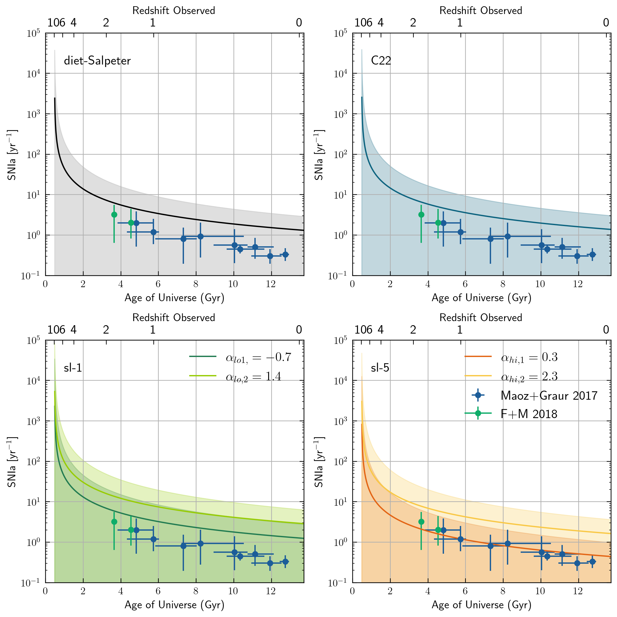
Figure 4: The delay-time-distribution derived for each IMF. The trends are compared with data from Friedmann & Maoz (2018) (F+M 2018) and Maoz & Graur (2017). Three of the DTDs over-predict the rate of SNIa, however they are still within $1\sigma$ (the shaded regions). Only the $\alpha_{hi,1}=0.3$ version of sl-5 (orange line of bottom-right plot) truly recreates the observed SNIa rate.

6.2 Best Fit IMF

IMF	$M_{br}$ ($M_{\odot}$)	$\alpha_{lo}$	$\alpha_{hi}$	$F$	$f^{Ia}$	$f^{CC}$
Low $M_{br}$	1.75	$-0.13\pm 0.24$	$0.53\pm 0.01$		$0.14\pm 0.005$	$0.86\pm 0.005$
	1.75	$0.20^{+0.74}_{-0.61}$	$0.96^{+0.59}_{-0.33}$	$0.47^{+0.22}_{-0.27}$	$0.27\pm 0.10$	$0.73\pm 0.10$
High $M_{br}$	6	$1.06\pm 0.11$	$0.53\pm 0.01$		$0.10\pm 0.01$	$0.90\pm 0.01$
	6	$0.18^{+0.76}_{-0.61}$	$1.15^{+0.74}_{-0.48}$	$0.44^{+0.17}_{-0.27}$	$0.56\pm 0.23$	$0.44\pm 0.23$

Table 3: Derived values for the best-fit IMFs and fractional values of SNIa and SNCC for the MCMC fit IMFs. Where a value of $F$ (fraction of the progenitor mass range $3-8M_{\odot}$ that become SNIa) is not defined it was not used as a free parameter in the MCMC.

Here we investigate the best-fit IMF parameters that derive a DTD which most closely fits the available data. There are three primary variables in the IMF: the low-mass slope ($\alpha_{lo}$), the high-mass slope ($\alpha_{hi}$), and the mass break between the two slopes ($M_{br}$). Ranges of each parameter are determined in L13 as these IMFs are shown to recreate $Z_{ICM}$: $-0.7<\alpha_{lo}<1.4$, $0.5<\alpha_{hi}<2.3$, and $0.5<M_{br}<8$. We ran a Markov Chain Monte Carlo (MCMC) to fit for the best IMF parameters using the listed variable ranges as hard prior limits as any deviation outside may result in non-physical $Z_{ICM}$ (L13). Fitting was done in log-space and the asymmetric errors on observational data from Maoz et al. (2010) and Friedmann & Maoz (2018) were averaged.

During initial fitting we found a degeneracy between $M_{br}$ and $\alpha_{lo}$. We held $M_{br}$ at constant values within the prior mass range and fit for $\alpha_{lo}$ and $\alpha_{hi}$, Figure 5. The value for $\alpha_{hi}$ is consistently fit within $1\sigma$ and we find a weighted average of $0.53\pm 0.01$. There are two $M_{br}$ ranges for consistently fit values of $\alpha_{lo}$. In $0.5<M_{br}/M_{\odot}<3$ we find a weighted average of $\alpha_{lo}=-0.13\pm 0.24$, and in $4<M_{br}/M_{\odot}<8$ the fit value increases to $\alpha_{lo}=1.06\pm 0.11$. Notably, the fit values associated with $M_{br}=6M_{\odot}$ produce an IMF that is closer to the one seen at present day (Salpeter, 1955). There is a transitional value of $\alpha_{lo}$ within the $M_{br}$ mass range $3-4M_{\odot}$ which we exclude from any averages. We proceed with calculations and DTD derivations using the two best-fit IMFs summarized in Table 3, and show the derived DTDs in Figure 6.

Our best constrained IMF parameters can be compared to a final observable value - the fractional amount of SNIa to SNCC ($f^{Ia}$ and $f^{CC}$, respectively) (see also Bulbul et al., 2012). The calculated supernovae ratios are summarized in Table 3. Our determined fractional amount of Ia is lower than what is found in the literature. L13 finds 20% of SNe are Ia using a diet-Salpeter IMF. Bulbul et al. (2012) use the spectral fitting model snapec to determine a fractional amount of SNIa in the range 30($\pm 5.4$)-37($\pm 7.1$)%. This is higher than our derived values, however this model assumes a Salpeter IMF. Observations find a value similar to ours, 8-15% (Mannucci et al., 2005), while studies of the ICM metallicity find 29-45% (Mernier et al., 2016). Our fit values for $M_{br}=1.75M_{\odot}$ most closely fit the literature value, while including an additional factor Notably, the variations in IMF sl-5 from L13 derive a $f^{ia}=7-97\%$ spanning the range of $f^{Ia}$ in the literature, and the best-fit values for $\alpha_{lo}$ and $\alpha_{hi}$.

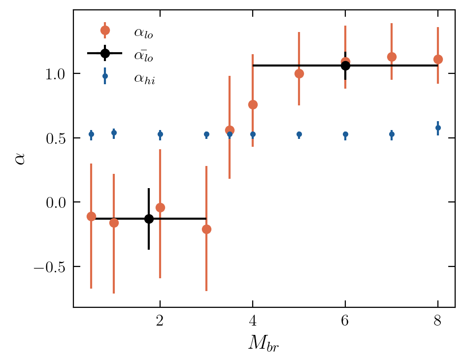
Figure 5: Fit values of $\alpha_{lo}$ (red data points) and $\alpha_{hi}$ (blue data points) with fixed values if $M_{br}$. The value for $\alpha_{hi}$ is consistent at $0.53\pm 0.01$ over the entire mass range. We find a weighted average value of $\alpha_{lo}=-0.13\pm 0.24$ within $0.5<M_{br}/M_{\odot}<3$ and $\alpha_{lo}=1.06\pm 0.11$ within $4<M_{br}/M_{\odot}<8$.

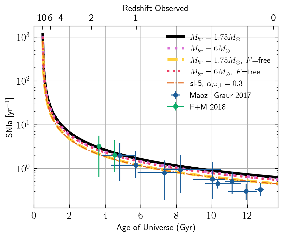
Figure 6: Best fit IMFs determined with an MCMC with $M_{br}=1.75M_{\odot}$ (black line), and $M_{br}=6M_{\odot}$ (purple dotted line). We allowed $F$ to be fit as a free parameter in the MCMC and show the fit results with $M_{br}=1.75M_{\odot}$ fitting $F=0.47^{+0.22}_{-0.27}$ (yellow dashed line), and $M_{br}=6M_{\odot}$ fitting $F=0.44^{+0.17}_{-0.15}$ (red dotted line). For comparison we plot sl-5 with $\alpha_{hi,1}=0.3$ from L13 (orange dash-dot line) which matches the fit with $M_{br}=1.75M_{\odot}$ and $F=0.47^{+0.22}_{-0.27}$. All fit results plotted are summarized in Table 3.

6.3 Fraction of stars that result in SNIa

An additional parameter to consider is the fractional amount of stars withing the progenitor mass range $3-8M_{\odot}$ that produce SNIa, $F$. This value is currently assumed to be 1, a likely incorrect assumption. We introduce $F$ as a free parameter in our MCMC fit and calculate the best-fit values for $F$, $\alpha_{lo}$ and $\alpha_{hi}$ holding $M_{br}=1.75M_{\odot}$ and $M_{br}=6M_{\odot}$.

The resulting MCMC with $M_{br}=1.75M_{\odot}$ gives best fit parameters $\alpha_{lo}=0.20^{+0.74}_{-0.61}$, $\alpha_{lo}=0.96^{+0.59}_{-0.33}$, and $F=0.47^{+0.22}_{-0.27}$. Holding $M_{br}=6M_{\odot}$ we fit for $\alpha_{lo}=0.18^{+0.76}_{-0.61}$, $\alpha_{hi}=1.15^{+0.74}_{-0.48}$, and $F=0.44^{+0.17}_{-0.27}$. These fits are also summarized in Table 3. The fit IMFs recreate the number of SNIa required and a DTD that is in agreement with those without allowing $F$ to be a free parameter, Figure 6. However, the errorbars on the fit parameters are larger by a factor of $\sim 2$ than any single MCMC fit excluding $F$ as a free parameter. This indicates that we have an insufficient amount of data available to confidently constrain the three IMF parameters and do not consider these IMFs as the best fit.

It is worth comparing the fit value of $F$ with a theoretical and more physically motivated calculation. Here we present an estimate calculation but recommend a full stellar evolutionary calculation be carried out to make sense of the true fraction.

There are three primary values needed for this estimation: fractional amount of stars in binary systems, fractional amount of binary systems with a period small enough to allow for mass transfer, fractional amount of binary systems within a mass range to form the binary without destroying the companion and allow for mass transfer. Multiplying each of these three fractional amount together results in the fractional amount of stars within the progenitor mass range that result in an SNIa.

Approximately 54%$\pm$3% of solar-type stars are single (assumed from a study of the Milky Way, Raghavan et al., 2010), therefore, we assume the remaining 46% of the stars to be in binary systems. The orbital period distribution can be described as Equation 4 where $P$ is the orbital period in days, $\overline{logP}$=4.8, $\sigma_{logP}$=2.3, and $Cst$ is a normalization constant that cancels out (Duquennoy & Mayor, 1991). Figure 1 in Moe & Di Stefano (2017) shows the expected period for binary systems that may turn into SNIa, $2<logP<3.7$. We integrate Equation 4 over the total binary population range, $0<logP<10$, and that expected for SNIa, finding the fractional amount of binary systems with $2<logP<3.7$ is 0.21 (21%).

$$f(logP)=Cst\>\text{exp}\Big{[}\frac{-(logP-\overline{logP})^{2}}{2\sigma^{2}_{logP}}\Big{]}$$ (4)

We use Equation 5 to determine the fractional number of binaries within a defined range of mass fractions, $q=M_{2}/M_{1}$, where $\mu=0.23$, and $\sigma_{q}=0.42$ (Duquennoy & Mayor, 1991). Figure 1 from Moe & Di Stefano (2017) presents $q$ that may result in SNIa as $0.1<q<0.3$. With this assumption we determine the fractional number of binaries with $0.1<q<0.3$ as 0.28 (28%).

$$f(q)=k\>\text{exp}\Big{[}\frac{-(q-\mu)^{2}}{2\sigma^{2}_{q}}\Big{]}$$ (5)

The resulting fractional amount of stars within the progenitor mass range to result in SNIa is $0.44\times 0.21\times 0.28=0.03$ (3%).

This is smaller than our previously determined $F$ of $\sim 0.45$ to match predictions with observations of SNIa. Maoz (2008) and Mannucci et al. (2008) both provide similar estimates of 2-40% of stars within the progenitor mass range 3-8$M_{\odot}$ and various IMF assumptions, with Maoz (2008) concluding 15% to be consistent with all assumptions. The difference in our higher, fit $F$ and lower, calculated values of $F$ may indicate that, for the EEP, the IMF and binary separation distribution was different than at low redshifts.

We conclude that our findings of $F$ are very unconstrained. Adding $F$ as a free parameter does not improve our derived IMF values, but the number of SNIa produced and DTD are properly derived. A lot is still unknown about SNIa pathways within nearby star systems, let alone at high-redshift as the EEP must have been.

7 Luminosity Functions

The hosts of the EEP are currently unknown, but are likely to be an early stellar population dominated by lower mass galaxies. Low optical luminosity dwarfs around the Milky Way present with an IMF (really a present-day mass function) that is flatter at masses $<$1 $M_{\odot}$ (Geha et al., 2015; Gennaro et al., 2018; Hansen et al., 2020), similar to a diet-Salpeter like is suggested for the EEP. A similar, shallow IMF is found in globular clusters (Cadelano et al., 2020), and low-mass, low-metallicity systems (Prgomet et al., 2022). In large systems such as galaxy clusters, these low- mass, luminosity, and metallicity systems are dwarf Elliptical (dE) galaxies, of which we see a large population (e.g., Blanton et al., 2005; Popesso et al., 2005; Trentham et al., 2005; Yamanoi et al., 2012). Here we posit these systems to be the original hosts of the EEP and investigate the consequences of different IMFs on the current state (remaining light) of the dE galaxies.

The luminosity function (LF) of galaxy clusters describes the number of galaxies at a given magnitude and is best described by a double Schechter function, each with a form described by Equation 6. Here $L_{*}$ is the turnover luminosity for a component, $\alpha$ is the slope, and $n_{*}$ is the space density normalization.

$$\Phi(L)dL=n_{*}(L/L_{*})^{\alpha}exp(-L/L_{*})d(L/L_{*})$$ (6)

The LF for galaxy clusters is unique as the LF for field galaxies, the Local Group and nearby groups can be described by a single Schechter component with a slope of $\alpha\approx 1.2$ over M(R)=-20 to M(R)=-10 (Lin et al., 1996; Phillipps et al., 1998; Trentham & Tully, 2002; Blanton et al., 2003).

The low-luminosity component in galaxy groups and clusters is dominated by dE galaxies. If one posits that these dE galaxies are some of the original hosts of the EEP, additional constraints may be placed on the IMF of the EEP. That is, for an assumed IMF, does the remaining light of the low-mass EEP stars exceed observations of dE galaxies in LFs? We investigate the importance of the dE galaxies and remnants of the EEP population by studying the LF of the Coma cluster.

7.1 Observed Luminosity

The Coma cluster luminosity function has been studied extensively over the past several decades in multiple filters and fields (i.e., Bernstein et al., 1995; Trentham, 1998; Adami et al., 2000; Andreon & Cuillandre, 2002; Mobasher et al., 2003; Milne et al., 2007; Yamanoi et al., 2012). Despite the many studies, there is still disagreement about the slope of the luminosity function for Coma, and indication for a steeper low-luminosity slope (de Propris et al., 1995). Differences between the studies may account for the inconsistencies. Some studies use spectroscopic redshift to identify cluster members, limiting the number of identifiable low-luminosity systems (Adami et al., 2000; Mobasher et al., 2003). Mobasher et al. (2003) covers $-23<M_{R}<-16$ and derives $\alpha=-1.18^{+0.04}_{-0.02}$ while Milne et al. (2007) finds $\alpha=-2.29\pm 0.33$ over $-14.58<M_{R}<-9.08$. The differences among these two magnitude ranges indicates two different powerlaw slopes for the high- and low-luminosity regimes.

We identify three works to analyze measurements, average, and fit a total LF of the Coma cluster for, Bernstein et al. (1995); Trentham (1998) and Milne et al. (2007). These papers cover a large range of magnitude in the R band ($-22<M_{R}<-9$), provide the apparent magnitude, and publish galaxy counts in comparable magnitude bins. The absolute magnitude is calculated by adopting a distance modulus of 34.83 (Trentham, 1998; Milne et al., 2007). Figure 7 shows the three LFs normalized to a 1^∘ field. We group the published counts into 0.5 magnitude bins, propagating errors, to determine an average LF for Coma, Figure 7.

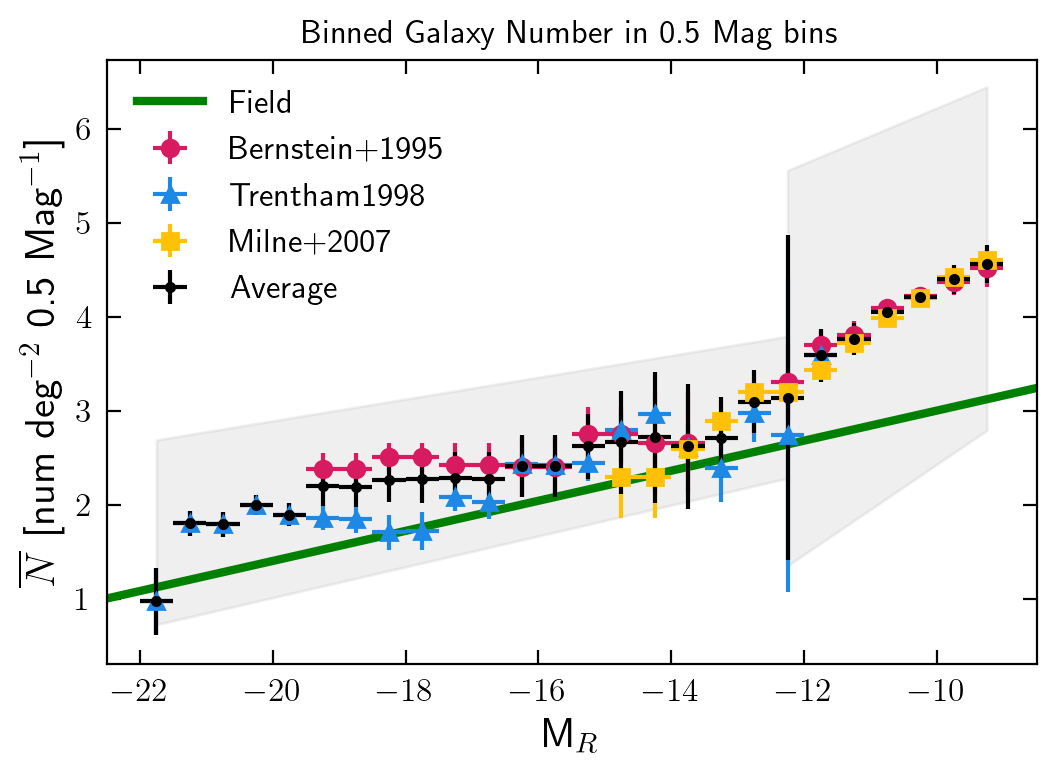
Figure 7: Luminosity function of Coma cluster from Bernstein et al. (1995); Trentham (1998); Milne et al. (2007) (red, blue, and yellow data points respectively). The averaged Coma LF is shown as the black points with $1\sigma$ errors (grey shaded region). We derive a powerlaw slope of $\alpha=-1.35\pm 0.06$ for $-22<M(R)<-12$ and $\alpha=-1.97\pm 0.23$ for $-12<M_{R}<-9$. There is a break in slope at $M_{R}\sim-12$. We plot the fit LF function trend for field galaxies with $\alpha=-1.4$ (solid green line) for comparison (Blanton et al., 2005). There is an excess of low-luminosity galaxies in the Coma LF compared to the field. All counts have been normalized to a 1^∘ field.

We follow the fitting method outlined in Yamanoi et al. (2012) to find the slope of the LF for the bright and faint components for Coma. The logarithmic slope of the luminosity function can be fit using linear regression as Equation 7 (Andreon & Cuillandre, 2002; Yamanoi et al., 2012).

$$log\phi=-0.4(\alpha+1)M+C$$ (7)

We use an MCMC to fit the logged luminosity function for $\alpha$ and the constant. Bootstrapping was used to determine the magnitude break between the high- and low-luminosity components as $M_{R}\sim-12$. The fit values were found to be $\alpha=-1.35\pm 0.06$ and $C=4.75\pm 0.46$ for $-22<M_{R}<-12$ and $\alpha=-1.97\pm 0.23$ and $C=8.20^{+0.98}_{-0.97}$ for $-12<M_{R}<-9$.

Absolute magnitude was converted to luminosity using a solar R-band absolute magnitude of 4.42. We then re-scale the 1^∘ normalized field as if it were observed within $R_{500}=47$ arcmin of Coma (Planck Collaboration et al., 2013). This radius was chosen to match our study of $Z_{ICM}$ versus $M_{*}/M_{gas}$ as the radius within which we calculate the expected luminosity from the remaining EEP. A Reimann sum was used to determine the cumulative luminosity for Coma in R-band within $R_{500}$, $9.14(\pm 1.94)\times 10^{12}$ $L_{\odot}$. For the bright galaxies ($M_{R}<-12$) the cumulative luminosity was calculated to be $8.98(\pm 1.93)\times 10^{12}$ $L_{\odot}$, and $1.63(\pm 0.62)\times 10^{11}$ $L_{\odot}$ for dim galaxies ($M_{R}>-12$).

7.2 Expected EEP Luminosity

The primary question to answer here is, does the light remaining by the EEP required to produce the missing metals exceed that seen in the dE galaxies of galaxy clusters? We test the four IMFs described in Table 2 and the best-fit IMFs in Table 3 (excliding $F$ as a free parameter) to see if they would create an excess light in the low-luminosity end of the Coma LF.

The following steps outline how we determine the cumulative luminosity for each :

1. Calculate the missing metal mass, that not explained by the visible stellar populations, of Coma ($M_{Z,EEP}$).

2. Determine the number of SNIa required to make $M_{Z,EEP}$.

3. Use the number of SNIa to normalize the IMF over the full mass range.

4. Assume the EEP formed as a burst at z=10. Stars with mass $<0.9M_{\odot}$ are still in existence today. Convert mass to luminosity using $L\propto M^{4}$ for stars with mass $<0.9M_{\odot}$.

5. Sum to determine the cumulative luminosity.

The cumulative luminosity calculated for each IMF is the total light remaining by stars from the EEP required to produce the measured ICM metallicity. We compare the cumulative luminosity determined from each IMF to the cumulative luminosity calculated for the low-luminosity part of the Coma LF ($1.63(\pm 0.62)\times 10^{11}$ $L_{\odot}$), $L_{dE,EEP}$. If the percentages are less than 100%, then all the remaining EEP light may be explained by the dE galaxies alone. The summary of calculated percentages for each IMF are shown in Table 4.

IMF	$L_{dE,EEP}$	$L_{dE,EEP}$ in bright galaxies
dS	199.1%	1.6%
C22	973.5%	14.1%
sl-1lo	271.9%	2.8%
sl-1hi	692.1%	9.6%
sl-5lo	15.2%	0%
sl-5hi	56.1%	0%
$M_{br}=1.75M_{\odot}$	26.2%	0%
$M_{br}=6M_{\odot}$	62.2%	0%

Table 4: Percent of light remaining for the EEP for each IMF. Column 1 presents the IMF tested. Column 2 is the percentage of dE light produced by the remaining EEP population. Column 3 is the percentage of remaining EEP light in the bright (-22$<$M(R)$<$-12) galaxies if the excess light from column 2 (anything in excess of 100%) merged into the bright galaxies. $F$ is not a free parameter in the two IMFs defined by $M_{br}$. The top 4 lines (3 models) are already ruled as unlikely by DTD predictions.

7.3 Comparison

Only IMFs sl-5, low-$M_{br}$ and high-$M_{br}$ (the two best-fit IMFs) produce few enough low-mass stars to not create an excess amount of light in the low-luminosity end of the Coma LF. However, galaxy clusters are dynamic systems that have gone through many mergers. We expect that some unknown fraction of dE galaxies that were initially home to the EEP have since merged with the brighter galaxies in the cluster. The question then becomes, if we assume some of these dE galaxies merged, what percentage of the high-luminosity cumulative light comes from $L_{dE,EEP}$? This value is calculated and shown in the third column of Table 4. C22 has the largest amount of excess EEP light ($L_{dE,EEP}=973.5\%$, and therefore the most light must be accounted for by the bright galaxies, 14.1%. We note that this value assumes that 100% of the dE light is from the EEP.

From the remaining light alone we cannot entirely rule out one of the 6 IMFs alone, or narrow down the three most likely IMFs (sl-5, and the two derived from MCMC fitting). Although C22 produces the most extreme values, the remaining EEP light may still be contained within the galaxy cluster without exceeding observations.

8 Summary

In this work we present example calculations of observable quantities for the theoretical Early Enrichment Population, DTD for Type Ia SNe and the remaining stellar luminosity. We use variations of IMFs that have been proven to reproduce the metallicity in the ICM for the predictions (Loewenstein, 2013; Corazza et al., 2022). Our findings can be summarized in the following points.

1. We calculate predicted delay-time-distributions (DTDs) for various IMFs, diet-Salpeter (dS), C22, sl-1 and sl-5. The DTDs from dS, C22 and sl-1 over-predict but are within $1\sigma$ of the observed SNIa rate (Maoz & Graur, 2017; Friedmann & Maoz, 2018). IMF sl-5 with $\alpha_{hi,1}=0.3$ most closely recreates the observations.

2. We use an MCMC to fit for the best IMF parameters, $\alpha_{lo}$, $\alpha_{hi}$ and $M_{br}$. We found a there to be two mass ranges within which $\alpha_{lo}$ was fit to a single value within $1\sigma$. The best fits are summarized in Table 3, and derived DTDs in Figure 6. These best-fit IMFs produce a fractional SNIa amount of $14\%\pm 0.5\%$ and $10\%\pm 1\%$ for a $M_{br}$ of 1.75 $M_{\odot}$ and 6 $M_{\odot}$ respectively. This lower than theoretical values such as 20% from L13 and 29-45% (Mernier et al., 2016).

3. We consider the addition of a factor $F$ to account for the fraction of stars within the progenitor mass range 3-8$M_{\odot}$ that go SNIa. We calculate a theoretical value of 3%, and find an MCMC best fit value of $0.47^{+0.22}_{-0.27}$ and $0.44^{+0.17}_{-0.15}$. Our lowest calculated values are in best agreement with those from the literature which produce a range of viable $F$ values of 2-40% (Mannucci et al., 2008; Maoz, 2008).

4. We look at constraining the low-mass end of the EEP IMF through remaining light in galaxy cluster luminosity functions (LF). We find that only sl-5 and the two best-fit IMFs reproduce an amount of remaining luminosity that may be contained by the dE population, 13-50% of the total dE light. However, the IMFs that over-predict dE light may not be entirely ruled out as we must consider merging of dE systems with the bright galaxies (-22$<$M(R)$<$-12). C22 predicts the contribution of remaining EEP light to the bright galaxies as 14%.

The IMF sl-5 from L13 with $\alpha_{hi,1}=0.3$ and the two derived best-fit IMFs seem to be the favorable IMFs as they recreate all present observations. There are a number of assumptions that may be better considered in future work with progress in fields such as merger tree histories for clusters and stellar evolution. Further observations of dE galaxies and SNIa in clusters will also help to better constrain current model fits.

References

- Adami et al. (2000) Adami, C., Ulmer, M. P., Durret, F., et al. 2000, A&A, 353, 930, doi: 10.48550/arXiv.astro-ph/9910217
- Andreon & Cuillandre (2002) Andreon, S., & Cuillandre, J. C. 2002, ApJ, 569, 144, doi: 10.1086/339261
- Antoniadis et al. (2020) Antoniadis, J., Chanlaridis, S., Gräfener, G., & Langer, N. 2020, A&A, 635, A72, doi: 10.1051/0004-6361/201936991
- Asplund et al. (2009) Asplund, M., Grevesse, N., Sauval, A. J., & Scott, P. 2009, ARA&A, 47, 481, doi: 10.1146/annurev.astro.46.060407.145222
- Baldi et al. (2012) Baldi, A., Ettori, S., Molendi, S., et al. 2012, A&A, 537, A142, doi: 10.1051/0004-6361/201117836
- Bernstein et al. (1995) Bernstein, G. M., Nichol, R. C., Tyson, J. A., Ulmer, M. P., & Wittman, D. 1995, AJ, 110, 1507, doi: 10.1086/117624
- Blackwell et al. (2022) Blackwell, A. E., Bregman, J. N., & Snowden, S. L. 2022, ApJ, 927, 104, doi: 10.3847/1538-4357/ac4dfb
- Blanton et al. (2005) Blanton, M. R., Lupton, R. H., Schlegel, D. J., et al. 2005, ApJ, 631, 208, doi: 10.1086/431416
- Blanton et al. (2003) Blanton, M. R., Hogg, D. W., Bahcall, N. A., et al. 2003, ApJ, 592, 819, doi: 10.1086/375776
- Bregman et al. (2010) Bregman, J. N., Anderson, M. E., & Dai, X. 2010, ApJ, 716, L63, doi: 10.1088/2041-8205/716/1/L63
- Bromm (2013) Bromm, V. 2013, Reports on Progress in Physics, 76, 112901, doi: 10.1088/0034-4885/76/11/112901
- Bromm & Loeb (2003) Bromm, V., & Loeb, A. 2003, Nature, 425, 812, doi: 10.1038/nature02071
- Bulbul et al. (2012) Bulbul, E., Smith, R. K., & Loewenstein, M. 2012, ApJ, 753, 54, doi: 10.1088/0004-637X/753/1/54
- Cadelano et al. (2020) Cadelano, M., Dalessandro, E., Webb, J. J., et al. 2020, MNRAS, 499, 2390, doi: 10.1093/mnras/staa2759
- Chantavat et al. (2023) Chantavat, T., Chongchitnan, S., & Silk, J. 2023, MNRAS, 522, 3256, doi: 10.1093/mnras/stad1196
- Chatzopoulos & Wheeler (2012) Chatzopoulos, E., & Wheeler, J. C. 2012, ApJ, 748, 42, doi: 10.1088/0004-637X/748/1/42
- Corazza et al. (2022) Corazza, L. C., Miranda, O. D., & Wuensche, C. A. 2022, A&A, 668, A191, doi: 10.1051/0004-6361/202244334
- De Grandi et al. (2004) De Grandi, S., Ettori, S., Longhetti, M., & Molendi, S. 2004, A&A, 419, 7, doi: 10.1051/0004-6361:20034228
- de Propris et al. (1995) de Propris, R., Pritchet, C. J., Harris, W. E., & McClure, R. D. 1995, ApJ, 450, 534, doi: 10.1086/176163
- Duquennoy & Mayor (1991) Duquennoy, A., & Mayor, M. 1991, A&A, 248, 485
- Elbaz et al. (1995) Elbaz, D., Arnaud, M., & Vangioni-Flam, E. 1995, A&A, 303, 345. https://arxiv.org/abs/astro-ph/9505107
- Fan et al. (2006) Fan, X., Carilli, C. L., & Keating, B. 2006, ARA&A, 44, 415, doi: 10.1146/annurev.astro.44.051905.092514
- Fang & Cen (2004) Fang, T., & Cen, R. 2004, ApJ, 616, L87, doi: 10.1086/426786
- Ferreras & Silk (2002) Ferreras, I., & Silk, J. 2002, MNRAS, 336, 1181, doi: 10.1046/j.1365-8711.2002.05863.x
- Flores et al. (2021) Flores, A. M., Mantz, A. B., Allen, S. W., et al. 2021, MNRAS, 507, 5195, doi: 10.1093/mnras/stab2430
- Freundlich & Maoz (2021) Freundlich, J., & Maoz, D. 2021, MNRAS, 502, 5882, doi: 10.1093/mnras/stab493
- Friedmann & Maoz (2018) Friedmann, M., & Maoz, D. 2018, MNRAS, 479, 3563, doi: 10.1093/mnras/sty1664
- Furnell et al. (2021) Furnell, K. E., Collins, C. A., Kelvin, L. S., et al. 2021, MNRAS, 502, 2419, doi: 10.1093/mnras/stab065
- Gal-Yam & Maoz (2004) Gal-Yam, A., & Maoz, D. 2004, MNRAS, 347, 942, doi: 10.1111/j.1365-2966.2004.07237.x
- Geha et al. (2015) Geha, M., Weisz, D., Grocholski, A., et al. 2015, ApJ, 811, 114, doi: 10.1088/0004-637X/811/2/114
- Gennaro et al. (2018) Gennaro, M., Tchernyshyov, K., Brown, T. M., et al. 2018, ApJ, 855, 20, doi: 10.3847/1538-4357/aaa973
- Ghizzardi et al. (2020) Ghizzardi, S., Molendi, S., van der Burg, R., et al. 2020, arXiv e-prints, arXiv:2007.01084. https://arxiv.org/abs/2007.01084
- Giallongo et al. (2014) Giallongo, E., Menci, N., Grazian, A., et al. 2014, ApJ, 781, 24, doi: 10.1088/0004-637X/781/1/24
- Grevesse & Sauval (1999) Grevesse, N., & Sauval, A. J. 1999, A&A, 347, 348
- Gursky et al. (1971) Gursky, H., Kellogg, E., Murray, S., et al. 1971, ApJ, 167, L81, doi: 10.1086/180765
- Gutierrez & Krawczynski (2005) Gutierrez, K., & Krawczynski, H. 2005, ApJ, 619, 161, doi: 10.1086/426420
- Hallman et al. (2018) Hallman, E. J., Alden, B., Rapetti, D., Datta, A., & Burns, J. O. 2018, ApJ, 859, 44, doi: 10.3847/1538-4357/aabf3a
- Hansen et al. (2020) Hansen, T. T., Marshall, J. L., Simon, J. D., et al. 2020, ApJ, 897, 183, doi: 10.3847/1538-4357/ab9643
- Heger & Woosley (2005) Heger, A., & Woosley, S. 2005, in IAU Symposium, Vol. 228, From Lithium to Uranium: Elemental Tracers of Early Cosmic Evolution, ed. V. Hill, P. Francois, & F. Primas, 297–302, doi: 10.1017/S1743921305005855
- Heger & Woosley (2002) Heger, A., & Woosley, S. E. 2002, ApJ, 567, 532, doi: 10.1086/338487
- Jaacks et al. (2019) Jaacks, J., Finkelstein, S. L., & Bromm, V. 2019, MNRAS, 488, 2202, doi: 10.1093/mnras/stz1529
- Kobayashi et al. (2006) Kobayashi, C., Umeda, H., Nomoto, K., Tominaga, N., & Ohkubo, T. 2006, ApJ, 653, 1145, doi: 10.1086/508914
- Krick & Bernstein (2007) Krick, J. E., & Bernstein, R. A. 2007, AJ, 134, 466, doi: 10.1086/518787
- Kroupa (2001) Kroupa, P. 2001, MNRAS, 322, 231, doi: 10.1046/j.1365-8711.2001.04022.x
- Laganá et al. (2013) Laganá, T. F., Martinet, N., Durret, F., et al. 2013, A&A, 555, A66, doi: 10.1051/0004-6361/201220423
- Lin et al. (1996) Lin, H., Yee, H. K. C., Carlberg, R. G., & Ellingson, E. 1996, JRASC, 90, 337
- Liu & Bromm (2020) Liu, B., & Bromm, V. 2020, arXiv e-prints, arXiv:2006.15260. https://arxiv.org/abs/2006.15260
- Liu et al. (2023) Liu, Z.-W., Roepke, F. K., & Han, Z. 2023, arXiv e-prints, arXiv:2305.13305, doi: 10.48550/arXiv.2305.13305
- Lodders (2021) Lodders, K. 2021, Space Sci. Rev., 217, 44, doi: 10.1007/s11214-021-00825-8
- Loewenstein (2001) Loewenstein, M. 2001, ApJ, 557, 573, doi: 10.1086/322256
- Loewenstein (2013) —. 2013, ApJ, 773, 52, doi: 10.1088/0004-637X/773/1/52
- Lovisari et al. (2020) Lovisari, L., Schellenberger, G., Sereno, M., et al. 2020, ApJ, 892, 102, doi: 10.3847/1538-4357/ab7997
- Mannucci et al. (2005) Mannucci, F., Della Valle, M., Panagia, N., et al. 2005, A&A, 433, 807, doi: 10.1051/0004-6361:20041411
- Mannucci et al. (2008) Mannucci, F., Maoz, D., Sharon, K., et al. 2008, MNRAS, 383, 1121, doi: 10.1111/j.1365-2966.2007.12603.x
- Mantz et al. (2017) Mantz, A. B., Allen, S. W., Morris, R. G., et al. 2017, MNRAS, 472, 2877, doi: 10.1093/mnras/stx2200
- Maoz (2008) Maoz, D. 2008, MNRAS, 384, 267, doi: 10.1111/j.1365-2966.2007.12697.x
- Maoz & Graur (2017) Maoz, D., & Graur, O. 2017, ApJ, 848, 25, doi: 10.3847/1538-4357/aa8b6e
- Maoz & Mannucci (2012) Maoz, D., & Mannucci, F. 2012, PASA, 29, 447, doi: 10.1071/AS11052
- Maoz et al. (2010) Maoz, D., Sharon, K., & Gal-Yam, A. 2010, ApJ, 722, 1879, doi: 10.1088/0004-637X/722/2/1879
- Matteucci & Calura (2005) Matteucci, F., & Calura, F. 2005, MNRAS, 360, 447, doi: 10.1111/j.1365-2966.2005.08908.x
- Mernier et al. (2016) Mernier, F., de Plaa, J., Pinto, C., et al. 2016, A&A, 595, A126, doi: 10.1051/0004-6361/201628765
- Million et al. (2011) Million, E. T., Werner, N., Simionescu, A., & Allen, S. W. 2011, MNRAS, 418, 2744, doi: 10.1111/j.1365-2966.2011.19664.x
- Milne et al. (2007) Milne, M. L., Pritchet, C. J., Poole, G. B., et al. 2007, AJ, 133, 177, doi: 10.1086/509733
- Mitchell et al. (1976) Mitchell, R. J., Culhane, J. L., Davison, P. J. N., & Ives, J. C. 1976, MNRAS, 175, 29P, doi: 10.1093/mnras/175.1.29P
- Mobasher et al. (2003) Mobasher, B., Colless, M., Carter, D., et al. 2003, ApJ, 587, 605, doi: 10.1086/368305
- Moe & Di Stefano (2017) Moe, M., & Di Stefano, R. 2017, ApJS, 230, 15, doi: 10.3847/1538-4365/aa6fb6
- Morsony et al. (2014) Morsony, B. J., Heath, C., & Workman, J. C. 2014, MNRAS, 441, 2134, doi: 10.1093/mnras/stu502
- Mushotzky et al. (1996) Mushotzky, R., Loewenstein, M., Arnaud, K. A., et al. 1996, ApJ, 466, 686, doi: 10.1086/177541
- Mushotzky et al. (1978) Mushotzky, R. F., Serlemitsos, P. J., Smith, B. W., Boldt, E. A., & Holt, S. S. 1978, ApJ, 225, 21, doi: 10.1086/156465
- Pallottini et al. (2014) Pallottini, A., Ferrara, A., Gallerani, S., Salvadori, S., & D’Odorico, V. 2014, MNRAS, 440, 2498, doi: 10.1093/mnras/stu451
- Phillipps et al. (1998) Phillipps, S., Driver, S. P., Couch, W. J., & Smith, R. M. 1998, ApJ, 498, L119, doi: 10.1086/311320
- Planck Collaboration et al. (2013) Planck Collaboration, Ade, P. A. R., Aghanim, N., et al. 2013, A&A, 554, A140, doi: 10.1051/0004-6361/201220247
- Planck Collaboration et al. (2016) Planck Collaboration, Adam, R., Aghanim, N., et al. 2016, A&A, 596, A108, doi: 10.1051/0004-6361/201628897
- Popesso et al. (2005) Popesso, P., Biviano, A., Böhringer, H., & Romaniello, M. 2005, in IAU Colloq. 198: Near-fields cosmology with dwarf elliptical galaxies, ed. H. Jerjen & B. Binggeli, 346–350, doi: 10.1017/S1743921305004035
- Portinari et al. (2004) Portinari, L., Moretti, A., Chiosi, C., & Sommer-Larsen, J. 2004, ApJ, 604, 579, doi: 10.1086/382126
- Prgomet et al. (2022) Prgomet, M., Rey, M. P., Andersson, E. P., et al. 2022, MNRAS, 513, 2326, doi: 10.1093/mnras/stac1074
- Raghavan et al. (2010) Raghavan, D., McAlister, H. A., Henry, T. J., et al. 2010, ApJS, 190, 1, doi: 10.1088/0067-0049/190/1/1
- Renzini & Andreon (2014) Renzini, A., & Andreon, S. 2014, MNRAS, 444, 3581, doi: 10.1093/mnras/stu1689
- Renzini et al. (1993) Renzini, A., Ciotti, L., D’Ercole, A., & Pellegrini, S. 1993, ApJ, 419, 52, doi: 10.1086/173458
- Salpeter (1955) Salpeter, E. E. 1955, ApJ, 121, 161, doi: 10.1086/145971
- Sarkar et al. (2022) Sarkar, A., Su, Y., Truong, N., et al. 2022, MNRAS, 516, 3068, doi: 10.1093/mnras/stac2416
- Sivanandam et al. (2009) Sivanandam, S., Zabludoff, A. I., Zaritsky, D., Gonzalez, A. H., & Kelson, D. D. 2009, ApJ, 691, 1787, doi: 10.1088/0004-637X/691/2/1787
- Thielemann et al. (1996) Thielemann, F.-K., Nomoto, K., & Hashimoto, M.-A. 1996, ApJ, 460, 408, doi: 10.1086/176980
- Thielemann et al. (1986) Thielemann, F. K., Nomoto, K., & Yokoi, K. 1986, A&A, 158, 17
- Trentham (1998) Trentham, N. 1998, MNRAS, 293, 71, doi: 10.1046/j.1365-8711.1998.01125.x
- Trentham et al. (2005) Trentham, N., Sampson, L., & Banerji, M. 2005, MNRAS, 357, 783, doi: 10.1111/j.1365-2966.2005.08697.x
- Trentham & Tully (2002) Trentham, N., & Tully, R. B. 2002, MNRAS, 335, 712, doi: 10.1046/j.1365-8711.2002.05651.x
- Urban et al. (2017) Urban, O., Werner, N., Allen, S. W., Simionescu, A., & Mantz, A. 2017, MNRAS, 470, 4583, doi: 10.1093/mnras/stx1542
- Werner & Mernier (2020) Werner, N., & Mernier, F. 2020, arXiv e-prints, arXiv:2001.10023. https://arxiv.org/abs/2001.10023
- Woosley (2017) Woosley, S. E. 2017, ApJ, 836, 244, doi: 10.3847/1538-4357/836/2/244
- Woosley & Heger (2015) Woosley, S. E., & Heger, A. 2015, Astrophysics and Space Science Library, Vol. 412, The Deaths of Very Massive Stars, ed. J. S. Vink, 199, doi: 10.1007/978-3-319-09596-7_7
- Yamanoi et al. (2012) Yamanoi, H., Komiyama, Y., Yagi, M., et al. 2012, AJ, 144, 40, doi: 10.1088/0004-6256/144/2/40
- Yang et al. (2015) Yang, Y. P., Wang, F. Y., & Dai, Z. G. 2015, A&A, 582, A7, doi: 10.1051/0004-6361/201525623
- Zibetti et al. (2005) Zibetti, S., White, S. D. M., Schneider, D. P., & Brinkmann, J. 2005, MNRAS, 358, 949, doi: 10.1111/j.1365-2966.2005.08817.x