DUST: A Framework for
Data-Driven Density Steering

Abstract

We consider the problem of data-driven stochastic optimal control of an unknown LTI dynamical system. Assuming the process noise is normally distributed, we pose the problem of steering the state’s mean and covariance to a target normal distribution, under noisy data collected from the underlying system, a problem commonly referred to as covariance steering (CS). A novel framework for Data-driven Uncertainty quantification and density STeering (DUST) is presented that simultaneously characterizes the noise affecting the measured data and designs an optimal affine-feedback controller to steer the density of the state to a prescribed terminal value. We use both indirect and direct data-driven design approaches based on the notions of persistency of excitation and subspace predictors to exactly represent the mean and covariance dynamics of the state in terms of the data and noise realizations. Since both the mean and the covariance steering sub-problems are plagued with distributional uncertainty arising from noisy data collection, we first estimate the noise realization from this dataset and subsequently compute tractable upper bounds on the estimation errors. The moment steering problems are then solved to optimality using techniques from robust control and robust optimization. Lastly, we present an alternative control design approach based on the certainty equivalence principle and interpret the problem as one of CS under multiplicative uncertainties. We analyze the performance and efficacy of each of these data-driven approaches using a case study and compare them with their model-based counterparts.

1 Introduction

The pursuit of safe and reliable control under uncertainties stands as a fundamental challenge in control theory. Traditional model-based techniques, such as the linear-quadratic regulator (LQR) or model-predictive control (MPC) have been extensively explored, and have been shown to be extremely effective at controlling dynamical systems when the model accurately represents the actual physical system. When there are model inaccuracies due to errors during system identification, robust control techniques [1] have been used to combat these inaccuracies and ensure robust constraint satisfaction and optimality under worst-case conditions. By the same token, exogenous disturbances affecting the state of a system have been treated in a multitude of ways; when the uncertainties are bounded, they fall under the realm of robust control [2]; when they are probabilistic they are treated with techniques from stochastic control [3].

Recently, there has been a paradigm shift from looking at control synthesis as an indirect design process of first estimating a model and subsequently solving an optimal control problem using the identified model, to a direct control design from raw data collected from the underlying physical system. This methodological shift has been inspired, among other things, by the early works on behavioral system theory by Willems et. al. [4], which showed that one can completely characterize the trajectory space of an LTI system by solely using raw data as long as this data is persistently exciting, a result known as the Fundamental Lemma. This data-driven formalism is attractive for a variety of reasons: firstly, it bypasses the technicalities and challenges of system identification methods which fail for complex models, and, instead, provides a direct end-to-end solution from data input to control output. Secondly, it is, in general, a more optimal scheme for control design [5]. More importantly, however, it provides a non-parametric dynamics model that is, by construction, adaptable to any linear system. As such, many of the traditional model-based control techniques have been re-explored within this data-driven context, with notable foundational works including DeePC [6, 7] and data-driven LQR [8, 9, 10].

The fundamental issue, however, with the use of Willems’ Fundamental Lemma in many applications stems from the fact that it only holds exactly for deterministic LTI systems. When the system is perturbed by bounded disturbances or is subject to stochastic dynamics or measurement noise, these direct data-driven schemes degrade rather quickly [11]. As a result, much of the recent work on this front has been tailored to exploring ways to robustify against noisy data. Notable methods along this line of research include suitably regularizing the optimization problem [12, 13], adding slack variables to account for data infeasibility [6, 7], and low-rank approximations of the data using truncated singular value decomposition [14, 15]. In fact, certain regularizers have a one-to-one correspondence with the corresponding indirect design methods, such as subspace predictive control (SPC), providing a bridge between the two approaches [16, 11]. Extensions such as $\gamma$-DeePC [17] and generalized-DeePC [18] have been proposed, which aim to bridge the gap between SPC and DeePC, benefiting from the positive aspects of both methods to tackle noisy data. In the context of direct state-feedback control design, techniques from robust control have been used to robustly stabilize all possible systems consistent with the data and perturbed by energy-bounded disturbances [19, 20].

The setting of stochastic predictive control, however, is far less studied, and the problem of designing optimal controllers for stochastic LTI systems under noisy data is much more challenging. Existing works on data-driven stochastic control adopt rather restrictive assumptions, such as noise-free offline data [21] or exact polynomial chaos expansions of stochastic measurements [22, 23]. A notable step towards a generalized framework for SPC is [24], where the authors explicitly quantify the statistical properties of error quantification from an indirect design based on noisy data, use a Kalman filter to estimate the initial condition, and reformulate the chance-constrained SPC problem as a semi-definite program (SDP).

In this work, we take a slightly different approach to the data-driven stochastic optimal control problem. We pose the control problem as one of steering the probability density of the state, as opposed to just the (mean) state vector. The canonical problem in this regard is to steer the state density of a linear system to some target Gaussian distribution subject to Gaussian disturbances and chance constraints. This problem has been solved exactly in both discrete-time [25, 26] and continuous-time [27, 28] settings, with demonstrated success in many engineering applications, such as spacecraft rendezvous [29], interplanetary trajectory optimization [30], and autonomous driving [31], to name a few. In the Gaussian setting, and since the state remains normally distributed for the entire horizon, the problem boils down to steering the first two moments of the state, hence the approach is often referred to as covariance steering (CS). Extensions of CS take into account the limiting linearity and additive Gaussianity assumptions, with recent works solving the density steering problem with non-Gaussian disturbances [32, 33], multiplicative and parametric disturbances [34, 35], distributional uncertainty [36, 37], and extensions to nonlinear systems [38, 39].

Our main contribution is the development of a general framework to steer the distribution of an unknown stochastic LTI system using raw data collected offline, instead of based on a known system model. We are interested in the so-called data-driven density steering (DD-DS) control problem and we develop a generalized framework to solve this problem, henceforth referred to as Data-driven Uncertainty quantification and density STeering (DUST). Since we will be dealing primarily with linear systems, we can, alternatively, investigate the data-driven mean steering (DD-MS) and data-driven covariance steering (DD-CS) problems. By combining model-based CS theory with behavioral systems theory and statistical learning, we provide a robust framework to steer both the mean and covariance of the state distribution to a desired terminal distribution. To this end, in Section 2, we firstly decompose the problem into one of data-driven mean steering (DD-MS) and one of data-driven covariance steering (DD-CS) as this framework allows for a separation principle for the individual moment trajectories, excluding the presence of constraints. From there, in Section 3, we follow an indirect certainty-equivalence route to exactly parameterize the mean dynamics in terms of the unknown noise realizations in the data, resulting in an uncertain quadratic program. For covariance control, we parameterize the feedback gains directly using the collected data and use established model-based CS theory to arrive at an uncertain SDP.

To handle the uncertainty during data collection, Section 4 develops novel noise estimation schemes to quantify the noise using techniques from maximum likelihood estimation, and neural networks. We then provide connections with the corresponding indirect design techniques. Using the known statistical properties from maximum likelihood estimation as well as quantitative notions of persistence of excitation, we construct high-confidence noise estimation error bounds in Section 5. These uncertainty bounds are then used in Section 6 to construct uncertainty sets and tractably reformulate the uncertain MS and CS problems as robust control and robust optimization problems, respectively, which can be solved efficiently to optimality using standard off-the-shelf solvers.

An illustrated flowchart of the proposed framework is shown in Figure 1.

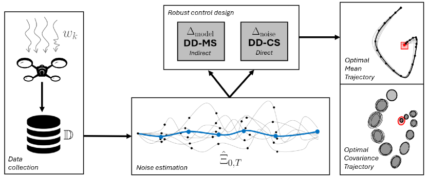
Figure 1: Breakdown of DUST framework into data-collection, noise estimation, and robust control. The noisy dataset $\mathbb{D}$ is used to estimate the past noise realization $\hat{\Xi}_{0,T}$, which is subsequently used to generate norm-bounded uncertainty sets $\Delta_{\mathrm{model}}$ for the (indirect) DD-MS and $\Delta_{\mathrm{noise}}$ for the (direct) DD-CS problems. The end result is optimal moment trajectories that satisfy terminal distributional constraints with high probability.

Since the noise enters multiplicatively in the indirect design formulation, we alternatively formulate a parametric uncertainty DD-DS (PU-DD-DS) problem and use convex relaxations to tractably solve the original problem in Section 7. Lastly, to illustrate the proposed framework, in Section 8 we perform an in-depth study of the proposed control design methods, analyzing their efficacy and precision, and compare them with their model-based counterparts. We conclude with a discussion of the proposed framework, and we offer several avenues for future extensions.

For reference, our previous work in [40] studied the limiting case of this problem, where the dynamics were assumed to be deterministic and the uncertainty resided solely in the boundary conditions. In this case, Willems Fundamental Lemma holds exactly, and we can achieve an exact correspondence with model-based designs. Our subsequent paper [41] studied the full data-driven density steering problem with noise quantification. However, in that work, the uncertainty sets were unnecessarily conservative (see Section 5). In this paper, we remove this restrictive assumption.

We remark that using the statistical properties of the noise for prediction and estimation is not unique to this work. Indeed, in the context of DeePC, recent methods such as the signal matrix model [42, 43] and Wasserstein estimation [44] have been proposed to find a relationship between past inputs/outputs and future outputs. Additionally, [45] extended these estimators to generate confidence sets, similar to our work, which can be used in the control design. Our work differs from these methods in the sense that we estimate the noise realizations (not just the statistics of the noise process) arising from the noisy data, from which we generate confidence sets for robust control. We also show that one can bypass all these estimation routines by treating the problem from a stochastic viewpoint and directly solve a stochastic optimal control problem with multiplicative uncertainties (Section 7).

1.1 Notation

Real-valued vectors are denoted by lowercase letters, $u\in\mathbb{R}^{m}$, matrices are denoted by upper-case letters, $V\in\mathbb{R}^{n\times m}$, and random vectors are denoted by boldface letters, $\boldsymbol{w}\in\mathbb{R}^{p}$. ${\mathchoice{\raisebox{0.0pt}{$\displaystyle\chi$}}{\raisebox{0.0pt}{$\textstyle\chi$}}{\raisebox{0.0pt}{$\scriptstyle\chi$}}{\raisebox{0.0pt}{$\scriptscriptstyle\chi$}}}^{2}_{p,q}$ denotes the inverse cumulative distribution function of the chi-square distribution with $p$ degrees of freedom and quantile $q$. The Kronecker product is denoted as $\otimes$ and the vectorization of a matrix $A$ is denoted as $\mathrm{vec}(A)=[a_{1}^{\intercal},\ldots,a_{M}^{\intercal}]^{\intercal}$, where $a_{i}$ is the $i$th column of $A$. We use the shorthand notation $[A;B]$ to denote the vertical stacking of two matrices or vectors of compatible dimension. We define the set $[\![T]\!]\triangleq\{1,\ldots,T\}$ and similarly $[\![T]\!]_{0}\triangleq\{0\}\cup[\![T]\!]$, for any natural number $T\in\mathbb{N}$. We denote the matrix two-norm by $\|\cdot\|$ and the matrix Frobenius norm by $\|\cdot\|_{\mathrm{F}}$. We denote the identity matrix of size $n\times n$ as $I_{n}$ and the zero matrix of size $m\times n$ as $0_{m\times n}$. For simplicity, we denote the $m$-long vector of zeros as $0_{m}$. Often, we will drop the subscript in these matrices if the dimension is clear from the context. Lastly, we succinctly denote a discrete-time signal $z_{0},z_{1},\ldots,z_{T}$ by $\{z_{k}\}_{k=0}^{T}$.

2 Problem Formulation

2.1 Problem Statement

We consider the following discrete-time stochastic time-invariant system

$$~{}\boldsymbol{x}_{k+1}=A\boldsymbol{x}_{k}+B\boldsymbol{u}_{k}+D\boldsymbol{w}_{k},$$ (1)

where $\boldsymbol{x}_{k}\in\mathbb{R}^{n}$ is the state, $\boldsymbol{u}_{k}\in\mathbb{R}^{m}$ is the control input, and $\boldsymbol{w}_{k}\sim\mathcal{N}(0,I_{d})$ are i.i.d. Gaussian disturbances, with time steps $k\in[\![N-1]\!]_{0}$, where $N$ represents the horizon length. Alternatively, we may re-write (1) as

$$~{}\boldsymbol{x}_{k+1}=A\boldsymbol{x}_{k}+B\boldsymbol{u}_{k}+\boldsymbol{\xi}_{k},$$ (2)

where $\boldsymbol{\xi}_{k}\sim\mathcal{N}(0,DD^{\intercal})$. The system matrices $A,B,D$ are assumed to be unknown. The initial uncertainty in the system resides in the initial state $\boldsymbol{x}_{0}$, which is a random $n$-dimensional vector drawn from the normal distribution

$$~{}\boldsymbol{x}_{0}\sim\mathcal{N}(\mu_{i},\Sigma_{i}),$$ (3)

where $\mu_{i}\in\mathbb{R}^{n}$ is the initial state mean and $\Sigma_{i}\in\mathbb{R}^{n\times n}\succ 0$ is the initial state covariance. It is assumed that the initial state is independent of the noise sequence, that is, $\mathbb{E}[\boldsymbol{x}_{0}\boldsymbol{w}_{k}^{\intercal}]=0$, for all $k\in[\![N-1]\!]_{0}$.

The objective is to steer the trajectories of (1) from the initial distribution (3) to the terminal distribution

$$~{}\boldsymbol{x}_{N}=\boldsymbol{x}_{f}\sim\mathcal{N}(\mu_{f},\Sigma_{f}),$$ (4)

where $\mu_{f}\in\mathbb{R}^{n}$ and $\Sigma_{f}\in\mathbb{R}^{n\times n}\succ 0$ are the desired state mean and covariance at time $N$, respectively. The cost function to be minimized is

$$~{}J(\boldsymbol{u})\triangleq\mathbb{E}\bigg{[}\sum_{k=0}^{N-1}(\boldsymbol{x}_{k}-x_{k}^{r})^{\intercal}Q_{k}(\boldsymbol{x}_{k}-x_{k}^{r})+\boldsymbol{u}_{k}^{\intercal}R_{k}\boldsymbol{u}_{k}\bigg{]},$$ (5)

where $\{x_{k}^{r}\}_{k=0}^{N-1}$ is a reference trajectory, and $Q_{k}\succeq 0$ and $R_{k}\succ 0$ for all $k\in[\![N-1]\!]_{0}$.

Remark 1.

We assume that the system (1) is controllable, that is, for any $x_{0},x_{f}\in\mathbb{R}^{n}$, and no noise ($w_{k}\equiv 0,~{}k\in[\![N-1]\!]_{0}$), there exists a sequence of control inputs $\{u_{k}\}_{k=0}^{N-1}$ that steer the system from $x_{0}$ to $x_{f}$.

It is assumed that we are given a $T$-long trajectory dataset $\mathbb{D}\triangleq\{x_{k}^{(d)},u_{k}^{(d)},x_{T}^{(d)}\}_{k=0}^{T-1}$ for control design. In the sequel, it is also possible to synthesize the controllers from multiple episodic datasets $\mathbb{D}_{\ell}$ ($\ell=1,\ldots,M$) but for simplicity, we assume only a single dataset in the present work. Lastly, we constrain the control law to have an affine state feedback form, parameterized by an open-loop control sequence $v=\{v_{k}\}_{k=0}^{N-1}$ and a feedback gain sequence $K=\{K_{k}\}_{k=0}^{N-1}$. In summary, the data-driven distribution steering (DD-DS) problem is stated below.

Problem 2 (DD-DS).

Given the collected dataset $\mathbb{D}$ corresponding to the unknown linear system (1), find the optimal control sequence $\{\boldsymbol{u}_{k}\}_{k=0}^{N-1}$ (equivalently, the feedforward $\{v_{k}\}_{k=0}^{N-1}$ and feedback gain $\{K_{k}\}_{k=0}^{N-1}$ sequences) that minimizes the objective function (5), subject to the initial state (3) and terminal state (4) boundary conditions.

2.2 Problem Reformulation

Borrowing from the work in [46], we adopt the control policy

$$~{}\boldsymbol{u}_{k}=K_{k}(\boldsymbol{x}_{k}-\mu_{k})+v_{k},$$ (6)

where $\mu_{k}=\mathbb{E}[\boldsymbol{x}_{k}]$ is the mean state, and where $K_{k}\in\mathbb{R}^{m\times n}$ controls the covariance of the state, and $v_{k}\in\mathbb{R}^{m}$ controls the mean of the state. Under the control law (6), and with complete system knowledge, it is possible to re-write Problem 2 as a convex program, which can be solved to optimality using off-the-shelf solvers [47].

With no chance constraints, and since the state distribution remains Gaussian at all time steps we decompose the system dynamics (1) into the mean dynamics and covariance dynamics. Plugging in the control law (6) into the dynamics (1) yields the decoupled dynamics

$$\mu_{k+1} =A\mu_{k}+Bv_{k},$$ (7a)

$$\Sigma_{k+1} =(A+BK_{k})\Sigma_{k}(A+BK_{k})^{\intercal}+DD^{\intercal}.$$ (7b)

As opposed to the approaches in [26, 25] that formulate a convex program in the lifted space of state and control trajectories, in this work, and similar to [46], we treat the moments of the intermediate states $\{\Sigma_{k},\mu_{k}\}_{k=0}^{N}$ over the steering horizon as decision variables in the resulting optimization problem.

Similar to the dynamics, the cost function (5) can be decoupled in terms of the first two moments as follows

$$J =J_{\mu}(\mu_{k},v_{k})+J_{\Sigma}(\Sigma_{k},K_{k}),$$ (8a)

$$J_{\mu} \triangleq\sum_{k=0}^{N-1}\Big{(}(\mu_{k}-x_{k}^{r})^{\intercal}Q_{k}(\mu_{k}-x_{k}^{r})+v_{k}^{\intercal}R_{k}v_{k}\Big{)},$$ (8b)

$$J_{\Sigma} \triangleq\sum_{k=0}^{N-1}\Big{(}\textrm{tr}(Q_{k}\Sigma_{k})+\textrm{tr}(R_{k}K_{k}\Sigma_{k}K_{k}^{\intercal})\Big{)}.$$ (8c)

Lastly, the two boundary conditions (3) and (4) are written as

$$\mu_{0}=\mu_{i},\quad\mu_{N}=\mu_{f},$$ (9a)

$$\Sigma_{0}=\Sigma_{i},\quad\Sigma_{N}=\Sigma_{f},$$ (9b)

where $\Sigma_{i},\Sigma_{f}\succ 0$. Problem 2 is now recast as the following two sub-problems.

Problem 3 (DD-MS).

Given the (unknown) mean dynamics (7a), find the optimal mean trajectory $\{\mu_{k}\}_{k=0}^{N}$ and the corresponding feed-forward control $\{v_{k}\}_{k=0}^{N-1}$ that minimize the mean cost (8b) subject to the boundary conditions (9a).

Problem 4 (DD-CS).

Given the (unknown) covariance dynamics (7b), find the optimal covariance trajectory $\{\Sigma_{k}\}_{k=0}^{N}$ and the corresponding feedback gains $\{K_{k}\}_{k=0}^{N-1}$ that minimize the covariance cost (8c) subject to the boundary conditions (9b).

Remark 5.

Under complete model knowledge, Problem 3 is a standard quadratic program with linear constraints that can be solved analytically given knowledge of the system matrices. Problem 4, however, is a non-linear and non-convex program due to the term $K_{k}\Sigma_{k}K_{k}^{\intercal}$ arising both in the cost function (8c) and the covariance dynamics (7b).

In the following section, we review the main concepts from behavioral systems theory [48] that will allow us to parametrize the decision variables in Problems 3 and 4 in terms of the collected input and output data streams.

3 Data-Driven Parameterization

We use concepts from behavioral systems theory to parametrize the decision variables of the control policy. First, recall the following definitions.

Definition 6.

Given a signal $\{z_{k}\}$ where $z_{k}\in\mathbb{R}^{\sigma}$, we denote the Hankel matrix of depth $\ell$ by

$$Z_{i,\ell,j}\triangleq\begin{bmatrix}z_{i}&z_{i+1}&\ldots&z_{i+j-1}\\ z_{i+1}&z_{i+2}&\ldots&z_{i+j}\\ \vdots&\vdots&\ddots&\vdots\\ z_{i+\ell-1}&z_{i+\ell}&\ldots&z_{i+\ell+j-2}\end{bmatrix}\in\mathbb{R}^{\sigma\ell\times j},$$ (10)

where $i\in\mathbb{Z}$ and $\ell,j\in\mathbb{N}$. For shorthand notation, if $\ell=1$, we denote the Hankel matrix by

$$Z_{i,1,j}\equiv Z_{i,j}=[z_{i}\ z_{i+1}\ \ldots\ z_{i+j-1}].$$ (11)

Definition 7.

The signal $\{z_{k}\}_{k=0}^{T-1}:[\![T-1]\!]_{0}\rightarrow\mathbb{R}^{\sigma}$ is persistently exciting of order $\ell$ if the matrix $Z_{0,\ell,j}$ with $j=T-\ell+1$ has rank $\sigma\ell$.

Suppose we carry out an experiment of duration $T\in\mathbb{N}$, where we collect input and noisy state data $\{u_{k}^{(d)}\}_{k=0}^{T-1}$ and $\{x_{k}^{(d)}\}_{k=0}^{T}$, respectively. Let the corresponding Hankel matrices for the input sequence, state sequence, and shifted state sequence (with $\ell=1$) be

$$U_{0,T} \triangleq[u_{0}^{(d)}\ u_{1}^{(d)}\ \ldots\ u_{T-1}^{(d)}],$$ (12a)

$$X_{0,T} \triangleq[x_{0}^{(d)}\ x_{1}^{(d)}\ \ldots\ x_{T-1}^{(d)}],$$ (12b)

$$X_{1,T} \triangleq[x_{1}^{(d)}\ x_{2}^{(d)}\ \ldots\ x_{T}^{(d)}].$$ (12c)

Assuming that the data is persistently exciting (PE), the block Hankel matrix of input and state data has full row rank

$$~{}\mathrm{rank}\begin{bmatrix}U_{0,T}\\ X_{0,T}\end{bmatrix}=n+m.$$ (13)

This PE assumption is crucial for direct data-driven control design, and is generally a mild assumption in practice, especially when noisy data is used [10]. The condition in (13) implies that any arbitrary input-state sequence of (1) can be expressed as a linear combination of the collected input-state data. Furthermore, as shown in the next section, this idea can be used [8] to parameterize any arbitrary feedback interconnection as well. In the following section, we parameterize the feedback gains in terms of the input-state data and reformulate the covariance steering problem as a semi-definite program (SDP).

3.1 Direct Data-Driven Covariance Steering (DD-CS)

From the rank condition (13), we can express the feedback gains as follows

$$~{}\begin{bmatrix}K_{k}\\ I_{n}\end{bmatrix}=\begin{bmatrix}U_{0,T}\\ X_{0,T}\end{bmatrix}G_{k},$$ (14)

where $G_{k}\in\mathbb{R}^{T\times n}$ are newly defined decision variables that provide the link between the feedback gains and the input-state data. Furthermore, using this data-driven parameterization, we can re-write the covariance dynamics (7b) as

$$\Sigma_{k+1} =[B\ \ A]\begin{bmatrix}K_{k}\\ I_{n}\end{bmatrix}\Sigma_{k}\begin{bmatrix}K_{k}\\ I_{n}\end{bmatrix}^{\intercal}[B\ \ A]^{\intercal}+DD^{\intercal}$$

$$=(X_{1,T}-\Xi_{0,T})G_{k}\Sigma_{k}G_{k}^{\intercal}(X_{1,T}-\Xi_{0,T})^{\intercal}+\Sigma_{\boldsymbol{\xi}},$$ (15)

where

$$X_{1,T}=AX_{0,T}+BU_{0,T}+\Xi_{0,T},$$ (16)

and where $\Xi_{0,T}\triangleq[\xi_{0}^{(d)},\ldots,\xi_{T-1}^{(d)}]\in\mathbb{R}^{n\times T}$ is the Hankel matrix of the (unknown) disturbances, and $\boldsymbol{\xi}_{k}^{(d)}\sim\mathcal{N}(0,\Sigma_{\boldsymbol{\xi}})$, where $\Sigma_{\boldsymbol{\xi}}\triangleq DD^{\intercal}$ is the covariance of the disturbance vector.

Similarly, the covariance cost (8c) can be re-written as

$$~{}J_{\Sigma,k}=\mathrm{tr}(Q_{k}\Sigma_{k})+\mathrm{tr}(R_{k}U_{0,T}G_{k}\Sigma_{k}G_{k}^{\intercal}U_{0,T}^{\intercal}).$$ (17)

To remedy the nonlinearity $G_{k}\Sigma_{k}G_{k}^{\intercal}$ in the covariance dynamics and the cost, define the new decision variables $S_{k}\triangleq G_{k}\Sigma_{k}\in\mathbb{R}^{T\times n}$, which yields

$$~{}\Sigma_{k+1}=(X_{1,T}-\Xi_{0,T})S_{k}\Sigma_{k}^{-1}S_{k}(X_{1,T}-\Xi_{0,T})^{\intercal}+\Sigma_{\boldsymbol{\xi}},$$ (18)

and

$$~{}J_{\Sigma,k}=\mathrm{tr}(Q_{k}\Sigma_{k})+\mathrm{tr}(R_{k}U_{0,T}S_{k}\Sigma_{k}^{-1}S_{k}^{\intercal}U_{0,T}^{\intercal}).$$ (19)

This problem is still non-convex due to the nonlinear term $S_{k}\Sigma_{k}^{-1}S_{k}^{\intercal}$. To this end, we relax the covariance dynamics by defining a new decision variable $Y_{k}\succeq S_{k}\Sigma_{k}^{-1}S_{k}^{\intercal}$, which yields the relaxed optimization problem

The equality constraint (20d) comes from the second block in (14) by multiplying $\Sigma_{k}$ on the right. The relaxed problem (20) is convex, since the constraints (20b) and (20c) can be written using the Schur complement in terms of the linear matrix inequalities (LMI)

$$\begin{bmatrix}\Sigma_{k}&S_{k}^{\intercal}\\ S_{k}&Y_{k}\end{bmatrix} \succeq 0,$$ (21a)

$$G_{\Sigma}^{k}\triangleq\begin{bmatrix}\Sigma_{k+1}-\Sigma_{\boldsymbol{\xi}}&(X_{1,T}-\Xi_{0,T})S_{k}\\ S_{k}^{\intercal}(X_{1,T}-\Xi_{0,T})^{\intercal}&\Sigma_{k}\end{bmatrix} \succeq 0.$$ (21b)

The cost (20a) and the equality constraints (20d)-(20e), on the other hand, are linear in all the decision variables, and hence are trivially convex.

3.2 Indirect Data-Driven Mean Steering (DD-MS)

Given the mean dynamics (7a) in terms of the open-loop control $v_{k}$, the PE condition (13) also provides a system identification type of result using the following theorem.

Theorem 8.

Suppose $\mathbb{D}=\{x_{k}^{(d)},u_{k}^{(d)},x_{T}^{(d)}\}_{k=0}^{T-1}$ is a dataset collected from the underlying system (1) such that the rank condition (13) holds. Then, the system (7a) has the following equivalent representation

$$~{}\mu_{k+1}=(X_{1,T}-\Xi_{0,T})\begin{bmatrix}U_{0,T}\\ X_{0,T}\end{bmatrix}^{\dagger}\begin{bmatrix}v_{k}\\ \mu_{k}\end{bmatrix}.$$ (22)

See [9] for details.

Remark 9.

Theorem 8 provides a data-based open-loop representation of a linear system. Assuming exact knowledge of the noise realization $\Xi_{0,T}$, one may equivalently interpret equation (22) as the solution to the least-squares problem

$$~{}\min_{B,A}\ \left\|X_{1,T}-\Xi_{0,T}-[B\ \ A]\begin{bmatrix}U_{0,T}\\ X_{0,T}\end{bmatrix}\right\|_{\mathrm{F}},$$ (23)

where $\|\cdot\|_{\mathrm{F}}$ is the Frobenius norm. Data-driven indirect designs based on the certainty-equivalence (CE) principle compute an approximate system description by solving (23) assuming no noise (i.e., $\Xi_{0,T}=0$).

Using Theorem 8, we can express the mean steering problem as the following convex problem

4 Noise Estimation Algorithms

The optimization problems (20) and (24), as they stand, albeit convex, are still intractable because we know neither the disturbance covariance $\Sigma_{\boldsymbol{\xi}}$ nor the noise realization history $\Xi_{0,T}$. The main subject of this paper, then, is to analyze various methods to make (20) and (24) tractable and, ultimately, satisfy the terminal mean and covariance constraints. In our previous work [40], we solved the noiseless DD-CS problem, where the uncertainty lies solely in the boundary distributions.

To this end, a natural starting point is to estimate the noise realization $\Xi_{0,T}$ and disturbance matrix $\Sigma_{\boldsymbol{\xi}}$ using the collected data. We propose two methods to recover these matrices: the first method estimates $\Xi_{0,T}$ and $\Sigma_{\boldsymbol{\xi}}$ using maximum likelihood (ML) estimation; the second method trains a feed-forward neural network (NN) to estimate both the disturbance and noise realization matrices. We illustrate these estimation techniques next.

4.1 ML Noise Estimation

To encode the stochastic linear system dynamics as a constraint we can use in the ML estimation scheme, we need to enforce consistency of the realization data. To this end, any realization of the dynamics (1) must satisfy (16). For notational convenience, next we denote the augmented Hankel matrix in (12) as

$$\mathcal{S}\triangleq\begin{bmatrix}U_{0,T}\\ X_{0,T}\end{bmatrix}\in\mathbb{R}^{(m+n)\times T},$$ (25)

from which we may re-write the dynamics realization as

$$X_{1,T}=[B\ A]\mathcal{S}+\Xi_{0,T}.$$ (26)

Additionally, noting that the matrix pseudoinverse satisfies the property $\mathcal{S}\mathcal{S}^{\dagger}\mathcal{S}=\mathcal{S}$, equation (16) can be written, equivalently, as

$$~{}X_{1,T}-\Xi_{0,T}=[B\ A]\mathcal{S}\mathcal{S}^{\dagger}\mathcal{S}.$$ (27)

Inserting the relation $X_{1,T}-\Xi_{0,T}=[B\ A]\mathcal{S}$ into the right-hand side of (27) yields

$$~{}(X_{1,T}-\Xi_{0,T})(I_{T}-\mathcal{S}^{\dagger}\mathcal{S})=0.$$ (28)

Equation (28) is a model-free type of condition that must be satisfied for all noisy linear system data realizations and hence is a consistency relation for any feasible set of data.

Given the constraint (28), the ML estimation problem then becomes

where $\rho_{\boldsymbol{\xi}}(\xi)$ is the probability density function (PDF) of the random vector $\boldsymbol{\xi}$, given as

$$~{}\rho_{\boldsymbol{\xi}}(\xi)=\frac{1}{(2\pi)^{n/2}}(\det\Sigma_{\boldsymbol{\xi}})^{-1/2}\exp\left(-\frac{1}{2}\xi^{\intercal}\Sigma_{\boldsymbol{\xi}}^{-1}\xi\right).$$ (30)

Remark 10.

Since the dynamics (1) are uncertain, it follows that there may be multiple noise realizations $\Xi_{0,T}$ that satisfy the linear dynamics. As such, the purpose of the constrained ML estimation (29) is to find the most likely sequence of noise realizations, $\hat{\Xi}_{0,T}$ from (29), given that the noise is normally distributed according to (30).

The next theorem provides the optimal solution to the maximum likelihood estimation (MLE) problem (29).

Theorem 11.

The solution to the MLE problem for the most probable noise realization $\Xi_{0,T}$ and disturbance covariance matrix $\Sigma_{\boldsymbol{\xi}}$ is given by

$$\Xi_{0,T}^{\star} =X_{1,T}(I_{T}-\mathcal{S}^{\dagger}\mathcal{S}),$$ (31a)

$$\Sigma_{\boldsymbol{\xi}}^{\star} =\frac{1}{T}X_{1,T}(I_{T}-\mathcal{S}^{\dagger}\mathcal{S})X_{1,T}^{\intercal}.$$ (31b)

The proof is given in Appendix A.

Remark 12.

The solution (31) of the MLE program in (29) is contingent on $\Sigma_{\boldsymbol{\xi}}\succ 0$. In fact, the optimal covariance estimate is simply the sample covariance of the dataset with respect to the estimated noise realizations, i.e., $\Sigma_{\boldsymbol{\xi}}^{\star}=\frac{1}{T}\Xi_{0,T}^{\star}(\Xi_{0,T}^{\star})^{\intercal}$. If $\Sigma_{\boldsymbol{\xi}}$ is singular, however, then $\log\det\Sigma_{\boldsymbol{\xi}}$ is undefined, hence the problem is infeasible. As a result, other methods, such as NN estimation (Section 4.2 below), or regularization techniques (e.g., GLASSO [49], distributionally-robust estimation [50]) should be used in these cases, instead. It should also be noted that such degenerate cases arise when the number of disturbance channels is less than the number of states channels, i.e., $D\in\mathbb{R}^{n\times d}$, with $d<n$.

4.2 NN Noise Estimation

An alternative way to estimate the realization noise given the data set $\mathbb{D}$ is by training a feed-forward neural network. To this end, let $f:\mathbb{R}^{n(T+1)+mT}\rightarrow\mathbb{R}^{nT}$ denote the NN mapping, where the input is $x\triangleq[x_{0}^{(d)^{\intercal}},x_{1}^{(d)^{\intercal}},\ldots,x_{T}^{(d)^{\intercal}}]^{\intercal},u_{0}^{(d)},\ldots,u_{T-1}^{(d)})$, and the output is $y\triangleq[\xi_{0}^{(d)^{\intercal}},\ldots,\xi_{T-1}^{(d)^{\intercal}}]^{\intercal}=\mathrm{vec}(\Xi_{0,T})$, respectively. Without loss of generality, we may consider a NN with ReLU activation functions. A ReLU NN transforms, at each layer $k$, the input as

$$x_{k}=f_{k}(x_{k-1})=\max(W_{k}x_{k-1}+b_{k},0),$$

where $W_{k}\in\mathbb{R}^{\ell_{k}\times\ell_{k-1}}$ is the weight and $b_{k}\in\mathbb{R}^{\ell_{k}}$ is the bias. Once an estimate, $\hat{\Xi}_{0,T}$, of the noise realization history is obtained, the noise covariance is computed simply as the sample covariance of the estimated data via (31b). It might also be possible to construct more elaborate networks to estimate both matrices of interest simultaneously.

In general, NN disturbance estimation is superior to MLE for a specific problem instance. However, as it is presented here, the learning scheme is supervised and relies on a noise realization output oracle, which is often not available in practice. Additionally, the network must be re-trained for different system dynamics, different data-collection horizon lengths $T$, and its performance is sensitive to the inputs one uses to collect the data. Clearly, the more persistently exciting the inputs $U_{0,T}$ are, the more the dynamics envelope of the system will be explored, and subsequently, the better the NN model will capture the actual system dynamics, thus providing better noise realization estimates. This connection between data informativeness and learning-based identification is an interesting topic for further exploration.

4.3 Indirect Design Estimation

We conclude this section by observing that an alternative to extracting disturbance information from the noisy data is by examining the difference between the observed state and the state prediction from the dynamics model. Referring to (2), and assuming knowledge of the system matrices $A$ and $B$, the disturbance would be given by

$$~{}\xi_{k}=x_{k+1}-Ax_{k}-Bu_{k},\quad k\in\mathbb{N}_{[0,T-1]}.$$ (32)

Given the collected data, and under the rank condition (13), an estimate $(\hat{B},\hat{A})$ of the system matrices can be obtained as the unique solution to the (noiseless) least-squares problem

$$~{}[\hat{B}\ \hat{A}]=\mathrm{argmin}_{B,A}\ \|X_{1,T}-[B\ A]\mathcal{S}\|_{\rm F}=X_{1,T}\mathcal{S}^{\dagger}.$$ (33)

Concatenating (32) over the entire sampling horizon yields the equality $\Xi_{0,T}=X_{1,T}-[B\ A]\mathcal{S}$. We may then estimate the noise sequence from the estimated model parameters in (33) as $\hat{\Xi}_{0,T}=X_{1,T}-[\hat{B}\ \hat{A}]\mathcal{S}$ or

$$~{}\hat{\Xi}_{0,T}=X_{1,T}(I_{T}-\mathcal{S}^{\dagger}\mathcal{S}),$$ (34)

from which we may compute the disturbance covariance as in (31b). The procedure, then, is to first estimate the nominal model, then estimate the disturbance structure, and lastly solve the associated CS problem using these estimated model parameters.

Notice that the optimal noise realization under the assumption of a noiseless system, (34), is equivalent to that of the optimal ML noise realization, (31a). Thus, the CE estimation is equivalent to the ML estimation under a known disturbance structure, implying that there may be deeper parallels between indirect and direct design methods in the context of noisy data. For an overview of this notion, please see [16].

In the following section, we present two methods to find bounds on the estimation error arising from the noise estimation techniques presented here. These estimation error bounds are then used to formulate (high-confidence) uncertainty sets in a robust control design in Section 6.

5 Uncertainty Set Synthesis

Given the noise estimation techniques outlined in Section 4, we now present two methods to derive bounds for the uncertainty estimation errors to be used later in the control design pipeline. As mentioned earlier, this is a necessary step to account for the model mismatch due to noisy data. The first method is based on the so-called Robust Fundamental Lemma (RFL) [51], which provides a stricter persistency of excitation condition, and guarantees bounded least-squares estimation errors for the indirect design. The second method, based on the ML noise estimation scheme, uses the statistical properties of the estimator to construct an upper bound on the estimation error with high confidence.

5.1 Robust Fundamental Lemma

Suppose we wish to identify the nominal model $\{A,B\}$ of (1) from the collected input/state data set $\mathbb{D}$. As mentioned in Section 4.3, an estimate $\{\hat{A},\hat{B}\}$ can be obtained as the unique solution to the least-squares problem (33). Furthermore, we know that the true system data satisfies the consistency relation (16). Thus, assuming $\sigma_{\min}(\mathcal{S})\neq 0$, the error of the model can be upper-bounded as

$$~{}\|[\hat{B}\ \hat{A}]-[B\ A]\|=\left\|\Xi_{0,T}\begin{bmatrix}U_{0,T}\\ X_{0,T}\end{bmatrix}^{\dagger}\right\|\leq\frac{\sigma_{\max}(\Xi_{0,T})}{\sigma_{\min}(\mathcal{S})}.$$ (35)

Since we do not have any control over the noise realization $\Xi_{0,T}$, we instead focus on the data matrix $\mathcal{S}$ defined in (25).

Definition 13 ([51], Quantitative PE).

Let $T>0,z_{k}:[\![T-1]\!]_{0}\rightarrow\mathbb{R}^{\sigma},\alpha>0$, and let $\ell>0$, with $T\geq\ell(\sigma+1)-1$. The input sequence $\{z_{k}\}_{k=0}^{T-1}$ is $\alpha$-persistency exciting of order $\ell$ if $\sigma_{\min}(Z_{0,\ell,T-1})\geq\alpha$.

Note that this is a direct generalization of the familiar PE condition in Definition 7. Indeed, any $\alpha$-PE input sequence of order $\ell$ is also PE of order $\ell$. Using this definition, the following theorem establishes sufficient conditions to lower bound the minimum singular value of $\mathcal{S}$.

Theorem 14 ([51], Robust Fundamental Lemma).

Let $T,\delta>0$ and assume that the pair $(A,B)$ is controllable. Define the square matrix

$$M\triangleq\begin{bmatrix}A&B&0_{n\times mn}\\ 0_{mn\times n}&0_{mn\times m}&I_{mn}\\ 0_{m\times n}&0_{m}&0_{m\times mn}\end{bmatrix},$$

and let $\mathcal{Z}=\{z=[\xi^{\intercal}\ \eta^{\intercal}\ 0_{nm}^{\intercal}]^{\intercal}\ |\ \xi\in\mathbb{R}^{n},\eta\in\mathbb{R}^{m},\|z\|=1\}$. Define, for $z\in\mathcal{Z}$, the matrix $\Theta_{z}\triangleq[z\ M^{\intercal}z\ \cdots\ (M^{\intercal})^{n}z]^{\intercal}$, and let $\kappa>0$ such that for all $z\in\mathcal{Z}$, $\sigma_{\min}(\Theta_{z})\geq\kappa$. Let $\{x_{k}^{(d)},u_{k}^{(d)},x_{T}^{(d)}\}_{k=0}^{T-1}$ be an input/state trajectory of (1) and let $\{\xi_{k}^{(d)}\}_{k=0}^{T-1}$ be the process noise realization. If $\{u_{k}^{(d)}\}_{k=0}^{T-1}$ is $\delta{\sqrt{n+1}}/{\kappa}$-persistently exciting or order $n+1$, then,

$$~{}\sigma_{\min}\left(\begin{bmatrix}U_{0,T}\\ X_{0,T}\end{bmatrix}\right)\geq\delta-\frac{\gamma\,\|\Xi_{0,n,T-2}\|}{\sqrt{n+1}},$$ (36)

where $\gamma>0$ is an upper bound on the norm of the matrix

$$\Phi_{\xi}\triangleq\begin{bmatrix}0&0&\cdots&0\\ \xi^{\intercal}&0&\cdots&0\\ \xi^{\intercal}A&\xi^{\intercal}&\cdots&0\\ \vdots&\vdots&\ddots&\vdots\\ \xi^{\intercal}A^{n-1}&\xi^{\intercal}A^{n-1}&\cdots&\xi^{\intercal}\end{bmatrix},$$

that is, $\|\Phi_{\xi}\|\leq\gamma$ for all $\xi\in\mathbb{R}^{n}$ such that $\|\xi\|\leq 1$,

In a nutshell, Theorem 14 says that if the input to the system satisfies the stricter PE condition of Definition 13, then we are guaranteed a lower bound on the minimum singular value of the input/state data Hankel matrix. This, in turn, provides an upper bound on the estimation error $[\Delta B\ \Delta A]\triangleq[B\ A]-[\hat{B}\ \hat{A}]$ in the indirect design method, which is used for the solution of the DD-MS problem. Alternatively, we can use this model error bound in the direct DD-CS design as follows.

First, re-write the realization dynamics (16) as

$$~{}X_{1,T}-(\Delta\Xi_{0,T}+\hat{\Xi}_{0,T})=([\hat{B}\ \hat{A}]+[\Delta B\ \Delta A])\mathcal{S},$$ (37)

where $\Delta\Xi_{0,T}\triangleq\Xi_{0,T}-\hat{\Xi}_{0,T}$. Further, by taking $\hat{\Xi}_{0,T}$ as the MLE solution in (31a), and $[\hat{B}\ \hat{A}]=X_{1,T}\mathcal{S}^{\dagger}$ as the CE estimated model, (37) yields

$$~{}\Delta\Xi_{0,T}=-[\Delta B\ \Delta A]\mathcal{S}.$$ (38)

Assuming now that the input sequence $\{u_{k}^{(d)}\}_{k=0}^{T-1}$ satisfies the conditions in Theorem 14 for some chosen $\delta>0$, we have that

$$\|\Delta\Xi_{0,T}\| \leq\|[\Delta B\ \Delta A]\|\|\mathcal{S}\|$$

$$\leq\frac{\sigma_{\max}(\Xi_{0,T})}{\delta-\gamma\|\Xi_{0,n,T-2}\|/\sqrt{n+1}}\|\mathcal{S}\|.$$ (39)

Thus, we obtain a bound of the form $\|\Delta\Xi_{0,T}\|\leq\rho(\delta)$, given the desired robustness level $\delta>0$.

Unfortunately, the estimation error upper bound (39) cannot be computed easily, due to the unknown noise realization $\Xi_{0,T}$ and the constant $\gamma$, which is a function of the system model $A$. However, it may be possible to upper bound these quantities. For example, using techniques from random matrix theory (RMT), it can be shown from the Sudakov-Fernique inequality [52] that

$$\mathbb{E}[\|\Xi_{0,T}\|]\leq\|\Sigma_{\boldsymbol{\xi}}^{1/2}\|(\sqrt{n}+\sqrt{T}).$$ (40)

The use of RMT to study the properties of the random data matrices arising from stochastic LTI systems is a fruitful avenue for future work.

5.2 Moment-Based Ambiguity Sets

In light of the discussion following (39), we are interested in practical bounds we can implement to ensure robust satisfaction of the constraints for the DD-MS and DD-CS problems. To do so, and equipped with the ML noise realization estimate (31a), we will use the statistical properties of $\hat{\Xi}_{0,T}$ and generate an ellipsoidal uncertainty set based on some degree of confidence $1-\delta\in[0.5,1)$. In the context of the control design problem, this will imply that the resulting controller will steer the system to the desired final distribution for all uncertainty estimates $\Delta\Xi_{0,T}\in\mathbf{\Delta}$, in some compact set $\mathbf{\Delta}$, with a prescribed degree of confidence $1-\delta$.

For simplicity, assume $\Sigma_{\boldsymbol{\xi}}\succ 0$ is known. First, we re-write the MLE problem (29) in terms of the vectorized parameters to be estimated $\xi\triangleq\mathrm{vec}(\Xi_{0,T})=[\xi_{0}^{\intercal},\cdots,\xi_{T-1}^{\intercal}]^{\intercal}\in\mathbb{R}^{nT}$ as

$$\min_{\xi} \mathcal{J}_{\mathrm{ML}}(\xi\ |\ \mathbb{D})=\frac{1}{2}\xi^{\intercal}(I_{T}\otimes\Sigma_{\boldsymbol{\xi}}^{-1})\xi$$ (41a)

$$C(\xi)\triangleq(\Gamma\otimes I_{n})\xi-\lambda=0,$$ (41b)

where $\Gamma\triangleq I_{T}-\mathcal{S}^{\dagger}\mathcal{S}\in\mathbb{R}^{T\times T}$, and $\lambda\triangleq\mathrm{vec}(X_{1,T}\Gamma)$. It can be shown [53] that, as the number of samples grows, the ML noise estimate $\hat{\xi}$ converges to a normal distribution as $\sqrt{T}(\xi-\hat{\xi})\overset{d}{\rightarrow}\mathcal{N}(0,\mathcal{I}^{-1})$, where $\mathcal{I}=\mathbb{E}_{\boldsymbol{\xi}}\left[\frac{\partial^{2}}{\partial\xi^{2}}\mathcal{J}_{\mathrm{ML}}(\xi\ |\ \mathbb{D})\right]$ is the Fisher Information Matrix (FIM), which is given by $\mathcal{I}=I_{T}\otimes\Sigma_{\boldsymbol{\xi}}^{-1}$ in the unconstrained case. For a constrained MLE problem, it can similarly be shown [54] that the asymptotic distribution of the estimate has covariance $\Sigma_{\Delta}=\mathcal{I}^{-1}-\mathcal{I}^{-1}J^{\intercal}(J\mathcal{I}^{-1}J^{\intercal})^{-1}J\mathcal{I}^{-1}$, where $J\triangleq\frac{\partial}{\partial\xi}C(\xi)=\Gamma\otimes I_{n}$ is the Jacobian of (41b). Using this ML estimation error covariance matrix, we can construct high-confidence uncertainty sets for use later in a robust control design (Section 6). To this end, we first compute the analytical form of the error covariance for the constrained MLE problem (29).

Lemma 15.

The distribution of the error of the constrained ML estimator (29) for the unknown noise realization $\xi=\mathrm{vec}(\Xi_{0,T})$ converges to the normal distribution $\mathcal{N}(0,\Sigma_{\Delta})$, where $\Sigma_{\Delta}=\mathcal{S}^{\dagger}\mathcal{S}\otimes\Sigma_{\boldsymbol{\xi}}$.

See Appendix B.

Given the noise estimation error covariance, we can construct an associated high confidence uncertainty set for the random matrix $\Delta\Xi_{0,T}$ by considering the quantile of the error distribution. To this end, we first present the original construction in [41] based on the full error covariance of the joint random vector $\Delta\xi=[\Delta\xi_{0}^{\intercal},\ldots,\Delta\xi_{T-1}^{\intercal}]^{\intercal}$. We then show that this uncertainty set is too loose, and its overapproximation does not scale intuitively with the sampling horizon $T$. To overcome these issues, we then present a novel uncertainty set synthesis scheme that generates more conservative, yet still feasible, upper bounds on the estimation error that is an order of magnitude smaller than the previous method in [41], yielding more tractable uncertainty sets for use in the robust control design of Section 6.

Proposition 16.

Assume that the uncertainty error estimate is normally distributed as $\Delta\xi\sim\mathcal{N}(0,\Sigma_{\Delta})$. Then, given some level of risk $\delta\in(0,0.5]$, the set $\mathbf{\Delta}=\{\|\Delta\Xi_{0,T}\|\leq\rho\}$, where $\rho=\frac{{\mathchoice{\raisebox{0.0pt}{$\displaystyle\chi$}}{\raisebox{0.0pt}{$\textstyle\chi$}}{\raisebox{0.0pt}{$\scriptstyle\chi$}}{\raisebox{0.0pt}{$\scriptscriptstyle\chi$}}}_{nT,1-\delta}}{\sqrt{\lambda_{\min}(\Sigma_{\Delta}^{-1})}}$ contains the $(1-\delta)$-quantile of $\Delta\Xi_{0,T}$, where ${\mathchoice{\raisebox{0.0pt}{$\displaystyle\chi$}}{\raisebox{0.0pt}{$\textstyle\chi$}}{\raisebox{0.0pt}{$\scriptstyle\chi$}}{\raisebox{0.0pt}{$\scriptscriptstyle\chi$}}}_{p,q}$ is the square root of the inverse of the ${\mathchoice{\raisebox{0.0pt}{$\displaystyle\chi$}}{\raisebox{0.0pt}{$\textstyle\chi$}}{\raisebox{0.0pt}{$\scriptstyle\chi$}}{\raisebox{0.0pt}{$\scriptscriptstyle\chi$}}}_{p,q}^{2}$ distribution.

See Appendix C.

Corollary 17.

For the MLE problem (29), the associated $(1-\delta)$-quantile uncertainty set $\mathbf{\Delta}=\{\|\Delta\Xi_{0,T}\|\leq\rho\}$ has the bound $\rho=\|\Sigma_{\boldsymbol{\xi}}^{1/2}\|{\mathchoice{\raisebox{0.0pt}{$\displaystyle\chi$}}{\raisebox{0.0pt}{$\textstyle\chi$}}{\raisebox{0.0pt}{$\scriptstyle\chi$}}{\raisebox{0.0pt}{$\scriptscriptstyle\chi$}}}_{nT,1-\delta}$.

See Appendix D.

In summary, using the MLE scheme (31) to estimate the unknown noise realizations of the LTI system (1) from the collected data $\mathbb{D}$, we are able to tractably compute a confidence ellipsoidal set $\mathbf{\Delta}$ from Corollary 17, to be used in the next section for (high-probability) robust satisfaction of the mean constraints (24b) and the covariance constraints (20c).

Notice, however, that due to the singularity of the error covariance matrix $\Sigma_{\Delta}$ (Lemma 15), the effective number of degrees of freedom is actually reduced. As a result, this naïve method overestimates the size of the uncertainty set by not accounting for the reduced variability dictated by the singular covariance matrix. This results in an unnecessarily conservative uncertainty bound compared to that of (44) in the following discussion. We first provide a formal definition of a normal distribution that takes into account singular covariance matrices.

Definition 18 ([55]).

Let $\mathbb{P}$ be a normal distribution on $\mathbb{R}^{p}$ with mean $\mu\in\mathbb{R}^{p}$ and covariance matrix $\Sigma\succeq 0$, that is, $\mathbb{P}=\mathcal{N}(\mu,\Sigma)$. Then, $\mathbb{P}$ is supported on $\mathrm{supp}(\mathbb{P})\triangleq\{\mu+Ev:v\in\mathbb{R}^{r}\}$, and its density with respect to the Lebesgue measure on $\mathrm{supp}(\mathbb{P})$ is given by

$$~{}\rho_{\mathbb{P}}(\xi)\triangleq\frac{1}{\sqrt{(2\pi)^{r}\det(D)}}e^{-\frac{1}{2}(\xi-\mu)^{\intercal}ED^{-1}E^{\intercal}(\xi-\mu)},$$ (42)

where $r=\mathrm{rank}(\Sigma),D\succ 0$ is the diagonal matrix of the positive eigenvalues of $\Sigma$, and $E\in\mathbb{R}^{p\times r}$ is the matrix whose columns correspond to the orthonormal eigenvectors of the positive eigenvalues of $\Sigma$.

Singular covariance matrices have no uncertainty along the eigenvectors corresponding to the zero eigenvalues. As a result, there is no probability density along these directions, and hence the density construction in Definition 18 defines a density on the $\mathrm{rank}(\Sigma)$-dimensional subspace through truncated diagonalization. We can now properly construct the confidence ellipsoid for a normal distribution with a singular covariance matrix by recognizing that $(\xi-\mu)^{\intercal}ED^{-1}E^{\intercal}(\xi-\mu)$ is a ${\mathchoice{\raisebox{0.0pt}{$\displaystyle\chi$}}{\raisebox{0.0pt}{$\textstyle\chi$}}{\raisebox{0.0pt}{$\scriptstyle\chi$}}{\raisebox{0.0pt}{$\scriptscriptstyle\chi$}}}^{2}$ random variable with $r$ degrees of freedom.

Proposition 19.

Given a normal distribution $\mathbb{P}=\mathcal{N}(\mu,\Sigma)$ with mean $\mu\in\mathbb{R}^{p}$ and covariance matrix $\Sigma\succeq 0$, the associated uncertainty set

$$~{}\mathcal{U}_{\mathcal{N}}\triangleq\{\xi\in\mathrm{supp}(\mathbb{P}):(\xi-\mu)^{\intercal}ED^{-1}E^{\intercal}(\xi-\mu)\leq\chi_{r,1-\delta}\}$$ (43)

contains the $(1-\delta)$-quantile of the distribution $\mathbb{P}$, that is, $\mathbb{P}(\xi\in\mathcal{U}_{\mathcal{N}})=1-\delta$.

The uncertainty set for the joint distribution $\Delta\xi$ from MLE can now be constructed by recognizing that $\mathrm{rank}(\Sigma_{\Delta})=n(n+m)$ since $\Sigma_{\Delta}=\mathcal{S}^{\dagger}\mathcal{S}\otimes\Sigma_{\boldsymbol{\xi}}$ from Lemma 15, and $\mathrm{rank}(S^{\dagger}\mathcal{S})=n+m$. Following a similar derivation as with Corollary 17, we arrive at the set

$$~{}\mathbf{\Delta}^{\star}=\{\|\Delta\Xi_{0,T}\|\leq\|\Sigma_{\boldsymbol{\xi}}^{1/2}\|{\mathchoice{\raisebox{0.0pt}{$\displaystyle\chi$}}{\raisebox{0.0pt}{$\textstyle\chi$}}{\raisebox{0.0pt}{$\scriptstyle\chi$}}{\raisebox{0.0pt}{$\scriptscriptstyle\chi$}}}_{n(n+m),1-\delta}\},$$ (44)

which guarantees that $\mathbb{P}(\Delta\Xi_{0,T}\in\mathbf{\Delta}^{\star})\geq 1-\delta$.

6 Robust DD-DS

Equipped with the machinery to efficiently estimate and bound the uncertainty due to the noise, we are now in a position to tackle the uncertain convex programs in (20) and (24). To this end, notice that the DD-MS problem essentially becomes a robust control problem with unstructured model uncertainty, albeit only with high probability guarantees. Hence, in Section 6.1, we use techniques from system-level synthesis (SLS) [56] to tractably enforce terminal constraint satisfaction (with high probability) for all bounded model uncertainties arising from the methods in Section 5. We note that this procedure is similar to the Coarse-ID proposed in [57], which used SLS to solve a robust control problem using uncertainty bounds constructed during the model identification step. Therein the authors employed techniques from RMT to construct tight uncertainty sets, which, as mentioned in Section 5.1, provide a promising framework for analyzing the estimation errors arising from both noise and model estimation. The main difference between our work and [57] is that we employ an indirect design technique solely for the mean steering problem, while other robust optimization methods, based on a direct design, are utilized to address the covariance steering problem. In this regard, the DD-CS problem requires robust satisfaction of LMI constraints along the planning horizon that encode the covariance propagation constraints under the chosen feedback control strategy. In Section 6.3, we will form the robust counterpart of these semi-infinite constraints, and use techniques from robust optimization to tractably enforce these as equivalent, deterministic LMIs.

6.1 Problem Formulation

Simply implementing the DD-MS program with the replacement $\hat{\Xi}_{0,T}\rightarrow\Xi_{0,T}$, will result in optimal controllers that do not satisfy the terminal constraint $\mu_{N}=\mu_{f}$ due to the inaccuracy in the estimated model from the indirect design step. The true mean dynamics are

$$\mu_{k+1}=(\hat{A}+\Delta A)\mu_{k}+(\hat{B}+\Delta B)v_{k},$$ (45)

where the nominal matrices $[\hat{B}\ \hat{A}]=X_{1,T}\mathcal{S}^{\dagger}$ are computed from CE estimation, and where the model deviations $\Delta A,\Delta B$ are bounded as $\|[\Delta B\ \Delta A]\|\leq\alpha(\delta)$, with $\alpha$ from (44) and (38).

Note, however, that enforcing the terminal constraint $\mu_{N}=\mu_{f}$ for all uncertainties $\|[\Delta B\ \Delta A]\|\leq\alpha$ is intractable, in general. Instead, we relax the pointwise terminal constraint to a terminal set given by a polytope such that $\mu_{N}\in\mathcal{X}_{f}\triangleq\{x:F_{x_{N}}x\leq b_{x_{N}}\}$, and require robust satisfaction of the constraint $\mu_{N}\in\mathcal{X}_{f}$, for all $\|\Delta A\|\leq\varepsilon_{A}$ and for all $\|\Delta B\|\leq\varepsilon_{B}$, for some $\varepsilon_{A},\varepsilon_{B}>0$. Along these lines, and in order to enhance tractability, we also impose polyhedral constraints on the transient of the mean state and the feed-forward input as $\mu_{k}\in\mathcal{X}_{k}\triangleq\{x:F_{x}x\leq b_{x}\}$ and $v_{k}\in\mathcal{U}_{k}\triangleq\{u:F_{u}u\leq b_{u}\}$. Lastly, instead of the open-loop control $v_{k}$, we introduce a feedback mean control in terms of the mean state history as follows $v_{k}=\sum_{i=0}^{k}L_{k,i}\mu_{i}$.

For notational convenience, let the nominal mean state be denoted by $\bar{\mu}_{k}$ which satisfies the error-free dynamics $\bar{\mu}_{k+1}=\hat{A}\bar{\mu}_{k}+\hat{B}\bar{v}_{k}$ and let $\bar{v}_{k}=\sum_{i=0}^{k}L_{k,i}\bar{\mu}_{i}$. In summary, the robust DD-MS (R-DD-MS) problem is posed as follows.

There are numerous methods in the robust control literature geared at tackling the R-DD-MS problem as posed in (46), ranging from the early works of tube-MPC [2] to disturbance-feedback with lumped uncertainty [58], to the more modern methods using system level synthesis (SLS) [56]. Below, we use SLS to solve the R-DD-MS problem by reformulating the semi-infinite program (46) as a tractable SDP.

6.2 Solution to the DD-MS Problem via SLS

The SLS approach to robust control aims at transforming the optimization problem over feedback control laws to one over closed-loop system responses, i.e., linear maps from the uncertainty process to the states and inputs in the closed loop. To this end, and for the nominal dynamics (46b), define the augmented state and control inputs as $\bar{\mu}=[\bar{\mu}_{0}^{\intercal},\cdots,\bar{\mu}_{N}^{\intercal}]^{\intercal},\bar{v}=[\bar{v}_{0}^{\intercal},\cdots,\bar{v}_{N}^{\intercal}]^{\intercal}$, and the vector $w\triangleq[\mu_{0}^{\intercal},0_{1\times n},\cdots,0_{1\times n}]^{\intercal}$. Let the control input $\bar{v}=L\bar{\mu}$, where

$$L=\begin{bmatrix}L_{0,0}&&&\\ L_{1,0}&L_{1,1}&&\\ \vdots&\ddots&\ddots&\\ L_{N,1}&\cdots&L_{N,N-1}&L_{N,N}\end{bmatrix},$$ (47)

and concatenate the dynamics matrices as $\hat{\mathcal{A}}\triangleq\mathrm{blkdiag}(I_{N},0)\otimes\hat{A}$ and $\hat{\mathcal{B}}\triangleq\mathrm{blkdiag}(I_{N},0)\otimes\hat{B}$. Let $Z\in\mathbb{R}^{n(N+1)\times n(N+1)}$ be the block-downshift operator, that is, a matrix with the identity matrix on the first block sub-diagonal and zeros elsewhere. Under the feedback controller $L$, the closed-loop behavior of the nominal system (46b) can be represented as

$$~{}\bar{\mu}=Z(\mathcal{A}+\mathcal{B}L)\bar{\mu}+w,$$ (48)

and the closed-loop map from $w\mapsto(\bar{\mu},\bar{v})$ is given by

$$~{}\begin{bmatrix}\bar{\mu}\\ \bar{v}\end{bmatrix}=\begin{bmatrix}(I-Z(\mathcal{A}+\mathcal{B}L))^{-1}\\ L(I-Z(\mathcal{A}+\mathcal{B}L))^{-1}\end{bmatrix}w=\begin{bmatrix}\bar{\Phi}_{x}\\ \bar{\Phi}_{u}\end{bmatrix}w,$$ (49)

where the matrices $\bar{\Phi}_{x}$ and $\bar{\Phi}_{u}$ are the nominal system responses under the action of the feedback controller $L$ in (47) on the LTI system (46b). The essence of the SLS approach is to treat these closed-loop system maps as the decision variables in the resulting optimization problem. In order to satisfy the closed-loop dynamics in (49), the matrices $\bar{\Phi}_{x}$ and $\bar{\Phi}_{u}$ must be constrained to an affine subspace parameterizing the system responses, similar to the subspace relations in (28) that encode the LTI dynamics of the realization data. The next theorem formalizes this intuition and provides the corresponding controller.

Theorem 20 ([56]).

Consider the nominal system dynamics (46b) with state feedback law $\bar{v}=L\bar{\mu}$, where $L$ is a block-lower triangular matrix. Then, the following are true:

• The affine subspace defined by

  $$~{}\begin{bmatrix}I_{(N+1)n}-Z\mathcal{A}&-Z\mathcal{B}\end{bmatrix}\begin{bmatrix}\bar{\Phi}_{x}\\ \bar{\Phi}_{u}\end{bmatrix}=I_{(N+1)n},$$ (50)

  parameterizes all possible system responses (49).

• For any block-lower triangular matrices $\bar{\Phi}_{x}$ and $\bar{\Phi}_{u}\}$ satisfying (50), the controller $L=\bar{\Phi}_{u}\bar{\Phi}_{x}^{-1}$ achieves the desired response.

See [56].

Thus, instead of requiring satisfaction of the dynamic constraints (46b), we can, equivalently, require satisfaction of the system map constraints (50) that achieve the desired system response. Moreover, this framework can be extended to handle model uncertainty as well, through the following theorem.

Theorem 21 ([56]).

Let $\bar{\Lambda}$ be an arbitrary block-lower triangular matrix, and suppose that $\Phi_{x}$ and $\Phi_{u}$ satisfy

$$~{}\begin{bmatrix}I-Z\mathcal{A}&-Z\mathcal{B}\end{bmatrix}\begin{bmatrix}\Phi_{x}\\ \Phi_{u}\end{bmatrix}=I-\bar{\Lambda}.$$ (51)

If $(I-\bar{\Lambda}_{i,i})^{-1}$ exists for all $i=0,\ldots,N$, then the controller $L=\Phi_{u}\Phi_{x}^{-1}$ achieves the system response

$$~{}\begin{bmatrix}\mu\\ v\end{bmatrix}=\begin{bmatrix}\Phi_{x}\\ \Phi_{u}\end{bmatrix}(I-\bar{\Lambda})^{-1}w.$$ (52)

See [56]. To see how Theorem 21 allows us to encode model uncertainty into the SLS framework, note that the nominal responses also approximately satisfy (50) with respect to the true model (46c) with an extra perturbation term given by

$$\begin{bmatrix}I-Z\mathcal{A}&-Z\mathcal{B}\end{bmatrix}\begin{bmatrix}\bar{\Phi}_{x}\\ \bar{\Phi}_{u}\end{bmatrix} =I-Z\begin{bmatrix}\Delta A&\Delta B\end{bmatrix}\begin{bmatrix}\bar{\Phi}_{x}\\ \bar{\Phi}_{u}\end{bmatrix}$$

$$\triangleq I-\Lambda\bar{\Phi}.$$ (53)

where in the first equality we use the fact that $\bar{\Phi}_{x}$ and $\bar{\Phi}_{u}$ satisfy (50), and in the second equality, we define $\bar{\Phi}\triangleq[\bar{\Phi}_{x};\bar{\Phi}_{u}]$, and $\Lambda\triangleq Z[\Delta A\ \Delta B]$. As a result, invoking Theorem 21 we conclude that the controller $L=\bar{\Phi}_{u}\bar{\Phi}_{x}^{-1}$, computed using only the system estimates $\{\hat{\mathcal{A}},\hat{\mathcal{B}}\}$, achieves the response (52) on the actual system $\{\mathcal{A},\mathcal{B}\}$, with $\bar{\Lambda}=\Lambda\bar{\Phi}$.

Next, we reformulate the objective function (46a) by equivalently re-writing it in terms of the augmented state and input as

$$\bar{\mathcal{J}}_{\mu} =\left\|\begin{bmatrix}\mathcal{Q}^{1/2}&0\\ 0&\mathcal{R}^{1/2}\end{bmatrix}\begin{bmatrix}\bar{\mu}\\ \bar{v}\end{bmatrix}\right\|^{2}-2\begin{bmatrix}\mathcal{Q}x^{r}\\ 0_{m}\end{bmatrix}^{\intercal}\begin{bmatrix}\bar{\mu}\\ \bar{v}\end{bmatrix}+\left\|\mathcal{Q}^{1/2}x^{r}\right\|^{2}$$

$$=\left\|\mathcal{M}^{1/2}\bar{\Phi}w\right\|^{2}-2\begin{bmatrix}\mathcal{Q}x^{r}\\ 0_{m}\end{bmatrix}^{\intercal}\bar{\Phi}w+\left\|\mathcal{Q}^{1/2}x^{r}\right\|^{2},$$ (54)

where $\mathcal{Q}\triangleq\mathrm{blkdiag}(Q_{0},\cdots,Q_{N}),\mathcal{R}\triangleq\mathrm{blkdiag}(R_{0},\cdots,R_{N})$, and $\mathcal{M}\triangleq\mathrm{blkdiag}(\mathcal{Q},\mathcal{R})$. Note that from the definition of $w$ the only non-zero entry in $w$ is its first block. Hence, by partitioning $\bar{\Phi}_{\star}=[\bar{\Phi}_{\star}^{0}\ \bar{\Phi}_{\star}^{\tilde{w}}]$, where $\star=x,u$, the cost (54) simplifies to

$$\bar{\mathcal{J}}_{\mu}=\left\|\mathcal{M}^{1/2}\bar{\Phi}^{0}\mu_{0}\right\|^{2}-2\begin{bmatrix}\mathcal{Q}x^{r}\\ 0_{m}\end{bmatrix}^{\intercal}\bar{\Phi}^{0}\mu_{0}+\left\|\mathcal{Q}^{1/2}x^{r}\right\|^{2}.$$ (55)

Similarly, we can simplify the uncertain system response in (52) as

$$\begin{bmatrix}\mu\\ v\end{bmatrix} =(\bar{\Phi}+\bar{\Phi}\Lambda(I-\bar{\Phi}\Lambda)^{-1}\bar{\Phi})w$$

$$=\bar{\Phi}^{0}\mu_{0}+\bar{\Phi}\Lambda(I-\bar{\Phi}\Lambda)^{-1}\bar{\Phi}^{0}\mu_{0},$$ (56)

where the first equality comes from the Woodbury matrix identity [59]. Lastly, we concatenate all the constraints $x_{k}\in\mathcal{X},u_{k}\in\mathcal{U},x_{N}\in\mathcal{X}_{f}$ together in the compact form $F[\mu;v]\leq b$, where $F\triangleq\mathrm{blkdiag}(F_{x},\cdots,F_{x},F_{x_{N}},F_{u},\cdots,F_{u})$ and $b\triangleq[b_{x}^{\intercal},\cdots,b_{x}^{\intercal},b_{x_{N}}^{\intercal},b_{u}^{\intercal},\cdots,b_{u}^{\intercal}]^{\intercal}$. In summary, the R-DD-MS problem (46) can be equivalently written as the following program

The main difficulty in (57) is in the robust constraints (57c), which are nonlinear in $\bar{\Phi}$. Following the work in [60], however, we can upper bound the LHS of the constraints and formulate sufficient conditions for which (57c) holds, for all $\|\Delta A\|\leq\varepsilon_{A}$ and $\|\Delta B\|\leq\varepsilon_{B}$. This convex approximation is stated in the following theorem.

Theorem 22.

Any controller synthesized from a feasible solution $\bar{\Phi}=[\bar{\Phi}_{x};\bar{\Phi}_{u}]=[\bar{\Phi}^{0}\ \bar{\Phi}^{\tilde{w}}]$ to the convex program

$$\min_{\bar{\Phi}_{x},\bar{\Phi}_{u}} \|\mathcal{M}^{1/2}\bar{\Phi}^{0}\mu_{0}\|_{2}^{2}$$ (58a)

$$\ \ \mathrm{s.t.} \begin{bmatrix}I-Z\hat{\mathcal{A}}&-Z\hat{\mathcal{B}}\end{bmatrix}\bar{\Phi}=I,$$ (58b)

$$F_{j}^{\intercal}\bar{\Phi}^{0}\mu_{0}+\|F_{j}^{\intercal}\bar{\Phi}^{\tilde{w}}\|\frac{1-\tau^{N}}{1-\tau}\gamma\leq b_{j},\ \forall j\in[\![J]\!],$$ (58c)

$$\left\|\begin{bmatrix}\frac{\varepsilon_{A}}{\alpha}\bar{\Phi}_{x}^{\tilde{w}}\\ \frac{\varepsilon_{B}}{1-\alpha}\bar{\Phi}_{u}^{\tilde{w}}\end{bmatrix}\right\|\leq\frac{\tau}{2},\quad\left\|\begin{bmatrix}\frac{\varepsilon_{A}}{\alpha}\bar{\Phi}_{x}^{0}\\ \frac{\varepsilon_{B}}{1-\alpha}\bar{\Phi}_{u}^{0}\end{bmatrix}\right\|\leq\frac{\gamma}{2},$$ (58d)

where $F_{j}\in\mathbb{R}^{(N+1)(n+m)},b_{j}\in\mathbb{R}$ denote the $j$th row and element of $F$ and $b$, respectively, with constants $\varepsilon_{A},\varepsilon_{B}>0$, and hyperparameters $\tau,\gamma>0,\alpha\in(0,1)$, guarantees constraint satisfaction under all possible model uncertainties in (46).

See Appendix E.

6.3 Solution of the Robust DD-CS Problem

In this section, we reformulate the uncertain CS program (20) so that is amenable to a tractable convex matrix feasibility problem. The original constraints $G_{k}^{\Sigma}\succeq 0$ in (20c), when reformulated as the LMI constraints (21b), may be robustly satisfied with high-probability (i.e., $\mathbb{P}(G_{k}^{\Sigma}\succeq 0)\geq 1-\delta)$), using the decomposition $\Xi_{0,T}=\hat{\Xi}_{0,T}+\Delta\Xi_{0,T}$ along with the established estimation error bounds, as the semi-infinite uncertain LMIs

$$~{}\hat{G}_{k}^{\Sigma}+\Delta G_{k}^{\Sigma}(\Delta\Xi_{0,T})\succeq 0,\quad\forall\|\Delta\Xi_{0,T}\|\leq\rho(\delta),$$ (59)

where,

$$\hat{G}_{k}^{\Sigma}=\begin{bmatrix}\Sigma_{k+1}-\Sigma_{\boldsymbol{\xi}}&(X_{1,T}-\hat{\Xi}_{0,T})S_{k}\\ S_{k}^{\intercal}(X_{1,T}-\hat{\Xi}_{0,T})^{\intercal}&\Sigma_{k}\end{bmatrix}$$ (60)

is the nominal covariance LMI, and

$$\Delta G_{k}^{\Sigma}=\begin{bmatrix}0_{n}&-\Delta\Xi_{0,T}S_{k}\\ -S_{k}^{\intercal}\Delta\Xi_{0,T}^{\intercal}&0_{n}\end{bmatrix}\succeq 0$$ (61)

is the perturbation to the covariance LMI. Next, we represent the perturbation matrix (61) as

$$\Delta G_{k}^{\Sigma}=L^{\intercal}(S_{k})\Delta\Xi_{0,T}^{\intercal}R+R^{\intercal}\Delta\Xi_{0,T}L(S_{k}),$$ (62)

where $L^{\intercal}(S_{k})\triangleq[0_{n,T};-S_{k}^{\intercal}]$ and $R^{\intercal}=[I_{n};0_{n}]$. Finally, using [61], we may equivalently represent the uncertain LMI (59) as the following standard LMI

$$\begin{bmatrix}\lambda I_{T}&\rho L(S_{k})\\ \rho L^{\intercal}(S_{k})&\hat{G}_{k}^{\Sigma}(\Sigma_{k},\Sigma_{k+1},S_{k})-\lambda R^{\intercal}R\end{bmatrix}\succeq 0,$$ (63)

in terms of the decision variables $S_{k},\lambda,\Sigma_{k}$ and $\Sigma_{k+1}$.

7 Parametric Uncertainty DD-CS

Instead of deriving bounds on the uncertainty $\Delta\Xi_{0,T}$ as outlined in Section 5, and subsequently performing a robust control design on the worst-case disturbance error entering the system dynamics as in Section 6, we can, instead, treat the parametric disturbances entering the system as probabilistic, since we know their exact distribution, that is, $\boldsymbol{\xi}_{k}^{(d)}\sim\mathcal{N}(0,DD^{\intercal})$.

In this case, we estimate the disturbance matrix $\hat{D}$ (equivalently, the disturbance covariance $\hat{\Sigma}_{\boldsymbol{\xi}}$), and solve a DD-CS problem with probabilistic, parametric uncertainties as shown in the sequel. Next, we formulate the parametric uncertainty DD-CS (PU-DD-DS) problem and propose a tractable solution for it.

For simplicity, we will assume that we have knowledge of the disturbance matrix $D$, equivalently, the covariance of the noise. Consider the linear dynamics (1) together with the exact data-driven model

$$~{}[B\ A]=(X_{1,T}-\Xi_{0,T})\begin{bmatrix}U_{0,T}\\ X_{0,T}\end{bmatrix}^{\dagger}=(X_{1,T}-\Xi_{0,T})\mathcal{S}^{\dagger}.$$ (64)

In practice, of course, we do not know the actual uncertainty realization $\Xi_{0,T}$, thus much of the effort in the previous sections was focused on providing a reasonable estimate $\hat{\Xi}_{0,T}$ (along with estimation errors) to be used in a robust control design. In PU-DD-CS, instead, we consider this exact data-driven representation of the nominal dynamics model (64) from a probabilistic perspective. We utilize the fact that each $\boldsymbol{\xi}_{k}^{(d)}\sim\mathcal{N}(0,DD^{\intercal})$, treating these noise vectors as random variables with known probability distributions rather than attempting to estimate their specific realization.

This probabilistic treatment of data collection noise allows us to design a controller that is inherently robust to the entire distribution of possible noise realizations, rather than being robustly optimized for a single estimated noise instance.

7.1 Solution of the PU-DD-CS Problem

The resulting dynamics with multiplicative uncertainty may be written as

$$\boldsymbol{x}_{k+1}=(\hat{A}+\Delta A(\Xi_{0,T}))\boldsymbol{x}_{k}+(\hat{B}+\Delta B(\Xi_{0,T}))\boldsymbol{u}_{k}+\boldsymbol{\xi}_{k}.$$ (65)

Let $\tau_{i}\in\mathbb{R}^{m}$ denote the $i$th row of $\mathcal{S}_{1}$ and $\sigma_{i}\in\mathbb{R}^{n}$ denote the $i$th row of $\mathcal{S}_{2}$. Since $\Xi_{0,T}=[\boldsymbol{\xi}_{0}^{(d)},\ldots,\boldsymbol{\xi}_{T-1}^{(d)}]$, the dynamics (65) may be written as

$$\boldsymbol{x}_{k+1}=\left[\hat{A}-\sum_{i=0}^{T-1}\boldsymbol{\xi}_{i}^{(d)}\tau_{i}^{\intercal}\right]\boldsymbol{x}_{k}+\left[\hat{B}-\sum_{i=0}^{T-1}\boldsymbol{\xi}_{i}^{(d)}\sigma_{i}^{\intercal}\right]\boldsymbol{u}_{k}+\boldsymbol{\xi}_{k}.$$ (66)

Forming the outer product $\tilde{\boldsymbol{x}}_{k+1}\tilde{\boldsymbol{x}}_{k+1}^{\intercal}$, where $\tilde{\boldsymbol{x}}_{k}:=\boldsymbol{x}_{k}-\mu_{k}$, and taking expectations yields the following expression for the covariance dynamics equation (66)

$$~{}\Sigma_{x_{k+1}}=\hat{\Sigma}_{x_{k+1}}+\Delta\Sigma_{x_{k+1}}^{(1)}+\Delta\Sigma_{x_{k+1}}^{(2)},$$ (67)

where,

$$\hat{\Sigma}_{x_{k+1}}=\hat{A}\Sigma_{x_{k}} \hat{A}^{\intercal}+\hat{A}\Sigma_{x_{k},u_{k}}\hat{B}^{\intercal}$$

$$+\hat{B}\Sigma_{x_{k},u_{k}}^{\intercal}\hat{A}^{\intercal}+B\Sigma_{u_{k}}B^{\intercal}+\Sigma_{\boldsymbol{\xi}},$$ (68a)

$$\Delta\Sigma_{x_{k+1}}^{(1)} =\sum_{i=0}^{T-1}\Big{(}\sigma_{i}^{\intercal}\Sigma_{x_{k}}\sigma_{i}+\sigma_{i}^{\intercal}\Sigma_{x_{k},u_{k}}\tau_{i}$$

$$\quad+\tau_{i}^{\intercal}\Sigma_{x_{k},u_{k}}^{\intercal}\sigma_{i}+\tau_{i}^{\intercal}\Sigma_{u_{k}}\tau_{i}\Big{)}\Sigma_{\boldsymbol{\xi}},$$ (68b)

$$\Delta\Sigma_{x_{k+1}}^{(2)}=\sum_{i=1}^{T-1} (\sigma_{i}^{\intercal}\mu_{k}+\tau_{i}^{\intercal}v_{k})(\sigma_{i}^{\intercal}\mu_{k}+\tau_{i}^{\intercal}v_{k})^{\intercal}\Sigma_{\boldsymbol{\xi}},$$ (68c)

where we have used the fact that the noise follows an i.i.d normal distribution and $\mathbb{E}[\boldsymbol{\xi}_{k}\boldsymbol{\xi}_{j}^{\intercal}]=\delta_{kj}I_{n}$ and $\mathbb{E}[\boldsymbol{\xi}_{i}^{(d)}\boldsymbol{\xi}_{k}^{\intercal}]=\delta_{ik}I_{n}$. With the affine feedback controller (6) the covariance matrices are given by

$$~{}\Sigma_{u_{k}}=K_{k}\Sigma_{x_{k}}K_{k}^{\intercal},\quad\Sigma_{x_{k},u_{k}}=\Sigma_{x_{k}}K_{k}^{\intercal}.$$ (69)

Note that with multiplicative uncertainties, the mean and covariance designs become coupled through the extra term (68c); this is in contrast to the case of only additive disturbances, where the mean and covariance subproblems are decoupled.

For the mean dynamics, we have the following exact representation

$$\mu_{k+1}=(\hat{A}+\Delta A(\Xi_{0,T}))\mu_{k}+(\hat{B}+\Delta B(\Xi_{0,T}))v_{k}.$$

To proceed, we follow an CE approach, by neglecting the model error matrices, which yields the approximate mean dynamics

$$~{}\mu_{k+1}\approx\hat{A}\mu_{k}+\hat{B}v_{k},$$ (70)

with the additional caveat that the terminal mean constraints will not be satisfied in practice, due to the model mismatch. Future work will investigate ways to incorporate robust design techniques, such as those in Section 6.1, in the context of PU-DD-DS. In summary, the PU-DD-DS problem is given as follows.

Problem 23 (PU-DD-DS).

Given the collected dataset $\mathbb{D}$ corresponding to the unknown linear system (1) with the nominal model $[\hat{B}\ \hat{A}]=X_{1,T}\mathcal{S}^{\dagger}$, find the optimal control sequence $\{\boldsymbol{u}_{k}\}_{k=0}^{N-1}$ that minimizes the cost (5), subject to the (approximate) mean and (exact) covariance dynamics (70), (67), initial state (3) and terminal boundary conditions $\mu_{N}=\mu_{f}$, $\Sigma_{N}\preceq\Sigma_{f}$.

Next, we provide a convex reformulation of Problem 23, which is similar to the derivation in [34]. To this end, first notice that the third term (68c) is quadratic in the decision variables $\{\mu_{k},v_{k}\}$. Additionally, the control parameterization (69) results in a nonlinear program in the decision variables $\{\Sigma_{u_{k}},K_{k},\Sigma_{x_{k}}\}$. To remedy the former issue, we relax the equality constraint (68c) by introducing the new decision variables $\Sigma_{ik}^{\Delta}$ such that

$$\Sigma_{ik}^{\Delta}\succeq(\sigma_{i}^{\intercal}\mu_{k}+\tau_{i}^{\intercal}v_{k})\Sigma_{\boldsymbol{\xi}}(\sigma_{i}^{\intercal}\mu_{k}+\tau_{i}^{\intercal}v_{k})^{\intercal},$$ (71)

which, using the Schur complement, can be recast as the LMI

$$\begin{bmatrix}\Sigma_{ik}^{\Delta}&\sigma_{i}^{\intercal}\mu_{k}+\tau_{i}^{\intercal}v_{k}\\ \sigma_{i}^{\intercal}\mu_{k}+\tau_{i}^{\intercal}v_{k}&\Sigma_{\boldsymbol{\xi}}^{-1}\end{bmatrix}\succeq 0.$$ (72)

To address the nonlinear dependence in the control parameterization, and in a similar manner to the theory developed in Section 2.1, define the new decision variables $U_{k}\triangleq K_{k}\Sigma_{x_{k}}=\Sigma_{x_{k},u_{k}}^{\intercal}$. The control covariance thus becomes $\Sigma_{u_{k}}=U_{k}\Sigma_{x_{k}}^{-1}U_{k}^{\intercal}$, which is still nonlinear in the decision variables. To this end, we relax this equality constraint by introducing yet another new decision variable $Y_{k}$ such that

$$Y_{k}\succeq U_{k}\Sigma_{x_{k}}^{-1}U_{k}^{\intercal}\implies\begin{bmatrix}Y_{k}&U_{k}\\ U_{k}^{\intercal}&\Sigma_{x_{k}}\end{bmatrix}\succeq 0.$$ (73)

In summary, the relaxed PU-DD-DS problem is given by the SDP in (74)

8 Numerical Example

To compare all previous methods, we use the following linear system from [62]

$$A=\frac{1}{2}\begin{bmatrix}1&-1\\ 2&1\end{bmatrix},\quad B=I_{2},\quad D=0.1I_{2}.$$

The initial state is normally distributed with mean $\mu_{0}=[2,10]^{\intercal}$ and $\Sigma_{0}=(1/3)^{2}I_{2}$, and the target terminal distribution has mean $\mu_{0}=0_{2\times 1}$ and $\Sigma_{f}=0.25\Sigma_{0}$. For the objective function, we set $Q=I_{2}$ and $R=10I_{2}$. For the robust mean design (Section 6.1) we set the terminal constraint set as $\mathcal{X}_{f}=\{x:|\mu_{f,i}-x_{i}|\leq 0.5\}$, where $x_{i}\in\mathbb{R}$ denotes the $i$th element of the state.

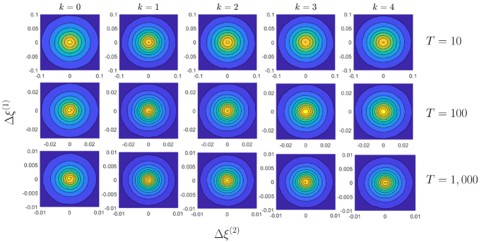
Figure 5: Empirical distribution of noise realization estimation errors $\Delta\xi_{k}$, for varying sampling horizons $T$. Each row corresponds to a different sampling horizon: $T=10$ (top row), $T=100$ (middle row), and $T=1,000$ (bottom row).

We start first with an analysis of the estimation errors $\Delta\Xi_{0,T}$ resulting from the MLE problem (29). To this end, we run the noise estimation procedure for $10^{6}$ random trials, where the data is randomly generated for each trial from inputs $\boldsymbol{u}_{k}^{(d)}\sim U[-1,1]$ and initial state $\boldsymbol{x}_{0}^{(d)}\sim\mathcal{N}(0,I_{2})$, and disturbances $\boldsymbol{w}_{k}^{(d)}\sim\mathcal{N}(0,DD^{\intercal})$. Figure 5 shows the distribution of the first five noise estimation errors $\Delta\xi_{k}$ for varying sampling horizon lengths $T\in\{10,100,1,000\}$. Notably, we see that, indeed, as we gather more noisy data, the covariance of the estimation errors of each individual noise term converges to its exact value, even though it is unknown. The total magnitude of the joint estimation error, $\|\Delta\Xi_{0,T}\|$, as shown in Figure 2, however, does not converge to zero. This is explained by noting that while the individual estimation errors converge with more samples, the compounded error remains fixed due to the increasing number of elements to be estimated. Additionally, Table 1 shows the efficacy of the various upper bounds constructed in Section 5.

Table 1: Upper bounds for noise uncertainty set constructions compared to true error quantile $\rho^{\star}$ for various confidence levels $\delta$.

$\delta$	0.1	0.2	0.3	0.4	0.5
$\rho^{\star}$	0.326	0.292	0.269	0.249	0.231
Tight	0.326	0.293	0.269	0.249	0.231
Loose $(T=10)$	0.533	0.500	0.477	0.458	0.440
Loose $(T=100)$	1.503	1.472	1.449	1.430	1.412

As mentioned, the uncertainty set (44) based on the subspace decomposition of the singular joint Gaussian density (Tight row) has the smallest conservativeness of all the three alternatives, as it is almost exactly equal to the true quantile. Additionally, the original uncertainty set construction (Loose row) in Corollary 17 provides unnecessarily too loose bounds, and degrades rather quickly for large sampling horizons. We thus confirm that the uncertainty set constructed from the subspace density has the tightest overapproximation to the true quantile, and the original construction in [41] is the most conservative due to the spurious extra degrees of freedom. For the rest of the analysis in this section, we choose to use the upper bound $\rho=\|\Sigma_{\boldsymbol{\xi}}^{1/2}\|{\mathchoice{\raisebox{0.0pt}{$\displaystyle\chi$}}{\raisebox{0.0pt}{$\textstyle\chi$}}{\raisebox{0.0pt}{$\scriptstyle\chi$}}{\raisebox{0.0pt}{$\scriptscriptstyle\chi$}}}_{n(n+m),1-\delta}$.

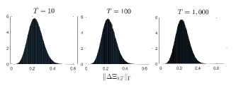
Figure 2: Empirical distribution of norm of joint estimation errors $\Delta\Xi_{0,T}$, for varying sampling horizons $T$.

Next, we turn to analyzing the effect of an unknown model on the resulting optimal mean trajectories. To this end, we compare the CE (i.e., using the subspace predictor $[\hat{B}\ \hat{A}]=X_{1,T}\mathcal{S}^{\dagger}$) design with the robust design outlined in Section 6.1. We remark that the ML noise estimation scheme in Section 4.1 does not influence the nominal model estimate since $\hat{\Xi}_{0,T}\mathcal{S}^{\dagger}=X_{1,T}(I_{T}-\mathcal{S}^{\dagger}\mathcal{S})\mathcal{S}^{\dagger}=0$. To compare the two designs, we run a set of 500 trials with data generated randomly for each trial in a similar vein to the noise estimation study. We use the upper bound $\alpha=\rho(\delta)/\sigma_{\min}(\mathcal{S})$ for the model estimation error with $\delta=0.1$ (as noted in Section 6) for the robust DD-MS design, and a data collection horizon $T=30$.

Figure 3 shows the difference between the optimal mean trajectories for the two designs with respect to the true model $\{A,B\}$.

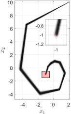
(a) R-DD-MS trajectories.

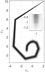
(b) DD-MS trajectories.

Figure 3: Comparison of (R)DD-MS optimal trajectories for 500 randomized trials of data collected from the true model over a horizon $T=30$.

Clearly, the robust design has better control over the dispersion of the terminal mean trajectories than that of the CE design, as intended. This can also be verified from Figure 7, which shows the terminal splashpoints of the mean state at the final time step.

To see how robust the two data-driven methods are to random models, not just simply comparing to a fixed known ground truth, we run only a single iteration of the data-collection and control design scheme with a fixed robustness level $\alpha=0.2$, and subsequently run the optimal mean controllers on 500 independent random models that are generated from the requirement $\|[B\ A]-[\hat{B}\ \hat{A}]\|\leq\alpha$. The resulting optimal mean trajectories are shown in Figure 4. Notably, the nominal mean controller now performs considerably worse when compared with that of the robust design on randomly perturbed models. In essence, Figures 3-4 show the robustness properties of DD-MS from two perspectives: the first shows robustness to random datasets on a known, underlying model, while the second shows robustness to a single dataset on randomly perturbed models.

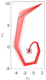
(a) R-DD-MS trajectories.

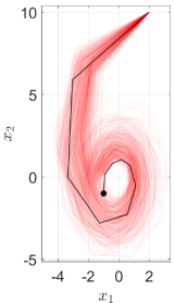
(b) DD-MS trajectories.

Figure 4: Comparison of (R)DD-MS optimal trajectories for 500 randomized trials of data collected from random models with $\|[\Delta B\ \Delta A]\|\leq\alpha$ over a horizon $T=30$.

For completeness, we would like to quantitatively understand the extent of conservatism of the bound $\alpha$ in R-DD-MS as well as the effect of the sampling horizon $T$ on the resulting nominal model inaccuracies. To this end, we run a series of one million random trials and computed $\alpha=\rho(\delta)/\sigma_{\min}(\mathcal{S})$ as well as the CE estimated model $[\hat{B}\ \hat{A}]=X_{1,T}\mathcal{S}^{\dagger}$ for each trial.

Table 2: Percentage of feasible solutions to R-DD-MC for varying model uncertainty $\delta$ and terminal constraint space size $|\mathcal{X}_{f}|$.

	Box Width
$\alpha$	0.5	0.4	0.3	0.2	0.1	0.05
0.05	1.000	1.000	1.000	1.000	1.000	0.994
0.1	1.000	1.000	1.000	1.000	0.962	0.506
0.15	1.000	1.000	1.000	1.000	0.438	0.174
0.2	1.000	1.000	1.000	0.710	0.134	0.080
0.25	1.000	0.994	0.424	0.084	0.062	0.046

Using this data, we plot the mean and variance of $\alpha$ as well as $\alpha^{\star}\triangleq\|[\Delta B\ \Delta A]\|$ for each risk level $\delta$ and for different sampling horizons $T$, as shown in Figure 6. For clarity, these dependencies are from the fact that $\rho$ is a function of $\delta$ and $\sigma_{\min}(\mathcal{S})$ is a function of $T$. We see that $\rho$ decreases with increasing $\delta$ due to a smaller confidence interval, and similarly $\sigma_{\min}(\mathcal{S})$ increases with $T$ due to a more expressive dataset. Indeed, the former point is the entire motivation for the robust fundamental lemma, which aims to quantitatively provide an upper bound on this increase. We see that, overall, the constructed uncertainty bounds provide a conservative, but tight, approximation to the true normed estimation error, and at 1,000 samples (red curve), we achieve an error of around 2% with respect to the true model with probability 95%. With smaller sample sizes (black curve), however, these errors get quite large with greater dispersions, and thus we see that robust mean designs are necessary for precise control with sparse data.

Finally, we wrap up the discussion on DD-MS design by focusing on the specific parameters involved, namely, the robustness level $\alpha$ and the terminal constraint box $\mathcal{X}_{f}$. One common issue with robust MPC frameworks is the design of the terminal set in order to ensure recursive feasibility [63]. In this work, however, we simply want a small enough terminal set, centered around the desired terminal mean that we can robustly steer the system trajectories to.

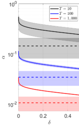
Figure 6: Model estimation error upper bounds (solid) and true estimation error (dashed).

As such, it is not guaranteed that the robust control problem will be feasible with a given terminal constraint set and model uncertainty $\alpha(\delta\ |\ \mathbb{D})$ under the dataset $\mathbb{D}$ and confidence level $\delta$. Table 2 shows a quantitative comparison of the percentage of feasible trajectories for varying levels of robustness and terminal set sizes. We see that when the terminal box is large and when there is not much robustness, all problems become feasible. However, as we increase the level of robustness and decrease the size of the terminal box, many more problems are infeasible. Thus, the control designer has a trade-off between the desired accuracy of the nominal model with the level of precision in the terminal state.

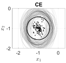
(a) Non-robust design.

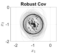
(b) Robust covariance design.

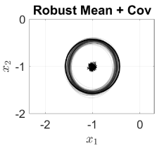
(c) Robust mean/covariance design.

Figure 7: Terminal state mean and covariances of (a) certainty-equivalence design, (b) CE mean design + robust covariance design, and (c) robust mean + covariance designs.

Next, we proceed with the DD-CS analysis in the presence of noisy data, and subsequently with the synthesis of both the mean and covariance control designs. To this end, and similarly to the DD-MS analysis, we first begin with a study on the effect of robustness level $\rho$ on the resulting terminal covariances. For reference, given the disturbance matrix $D=0.1I_{2}$, confidence level $\delta=0.1$, and sampling horizon $T=30$, the associated ML noise error uncertainty set is $\mathbf{\Delta}=\{\|\Delta\Xi_{0,T}\|\leq\rho\}$, with $\rho=0.3263$. Figure 8 shows the terminal covariances from the R-DD-CS design for varying levels of $\rho\in\{0,0.3,0.6,0.9,1.2,1.5\}$, as well as for varying noise-to-precision ratio (NPR) $\sigma_{\xi}/\sigma_{f}\in\{0.6,0.72,0.84,0.96\}$, evaluated on the true dynamics model $\{A,B,D\}$, where we assume $\Sigma_{f}=\sigma_{f}^{2}I_{2}$ and $\Sigma_{\boldsymbol{\xi}}=\sigma_{\boldsymbol{\xi}}^{2}I_{2}$. As the level of robustness to noise estimation errors increases, the terminal covariances become smaller when simulated on the true model because the optimal feedback gains anticipate more uncertainty than there is in reality.

Table 3: Percentage of feasible solutions to R-DD-CS for varying noise estimation error bounds $\delta$ and disturbance variance $\sigma_{\boldsymbol{\xi}}^{2}$.

	Noise variance $\sigma_{\boldsymbol{\xi}}^{2}$
$\rho$	$0.1^{2}$	$0.12^{2}$	$0.14^{2}$	$0.16^{2}$
0.0	1.000	1.000	1.000	1.000
0.3	1.000	1.000	1.000	1.000
0.6	1.000	1.000	1.000	0.040
0.9	1.000	0.990	0.708	0.000
1.2	0.870	0.542	0.010	0.000
1.5	0.228	0.012	0.000	0.000

Note also that with no robustness (i.e., $\rho=0$), the terminal covariances (black) do not, in general, satisfy the constraints (green) due to the non-zero estimation errors. Hence, robustness against estimation errors is essential for feasible covariance designs.

It is interesting to note that as the NPR increases, not only does the terminal covariance becomes larger, as expected, but also the R-DD-CS is more likely to become infeasible. According to [64], there is a theoretical lower bound on the achievable terminal covariance, given by $\Sigma_{N}\succeq D_{N-1}D_{N-1}^{\intercal}$. As the noise covariance $\sigma_{\xi}$ increases and approaches $\sigma_{f}$, this lower bound becomes more constraining. Simultaneously, increasing the robustness level $\rho$ requires the covariance steering algorithm to aim for smaller values of $\Sigma_{N}$ to ensure $\Sigma_{N}\preceq\Sigma_{f}$ holds for all bounded errors within $\rho$. However, when $\rho$ becomes too large relative to the gap between $\sigma_{\xi}$ and $\sigma_{f}$, the convex program becomes infeasible as it cannot reduce $\Sigma_{N}$ below the theoretical lower bound while meeting the robustness constraints. Table 3 empirically verifies this relationship, showing the percentage of feasible solutions for each NPR across 500 random trials.

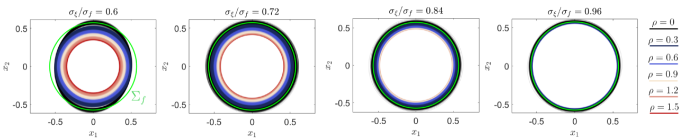
Figure 8: Terminal $3\sigma$ covariance ellipses for varying levels of robustness $\rho$ and desired precision to noise ratio $\sigma_{f}/\sigma_{\xi}$.

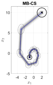
(a) Model-based DS.

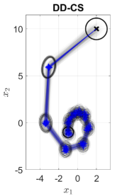
(b) Data-driven DS.

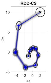
(c) Robust DD-DS.

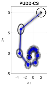
(d) Parametric uncertainty DD-DS.

Figure 9: Comparison of optimal trajectories between (a) model-based control design, and (b-d) data-driven control design.

Lastly, we combine the DD-MS and DD-CS designs together and look at the resulting optimal trajectories. We choose a planning horizon of $N=10$ and run a set of 50 random trials for data collection, where, for each trial, we plot 10 Monte Carlo trajectories from randomly sampling the additive noise. Of all the designs, the R-DD-DS design performs the best in terms of achieving the closest terminal distribution to the desired one in the presence of noisy data. The PU-DD-DS design, which does not estimate the noise realizations but instead incorporates the distributional knowledge as multiplicative uncertainty, satisfies the terminal covariances for each trial, but is not robust against mean estimation errors, similar to vanilla DD-MS. Figuring out a way to robustly satisfy the terminal mean constraints in this parametric uncertainty framework is an open problem for future work.

8.1 Discussion and Open Problems

In terms of semantics, we wonder whether the DD-CS design solution, in which we estimate the noise realization from the dataset and subsequently solve a convex program for the optimal feedback controller, is, in fact, a direct method. While we parameterize the feedback gains in terms of the data in (14) in terms of the decision variables $G_{k}$, this required intermediate step of estimating the noise realization (via MLE, for example) $\hat{\Xi}_{0,T}$ is essential to generate an uncertainty set $\{\|\Delta\Xi_{0,T}\|\leq\rho\}$ for terminal constraint satisfaction with high probability. In essence, this noise estimation procedure is akin to filtering the noisy signal, and it could be possible that there are connections with optimal state estimation. We leave it as an open problem to design a feedback controller that satisfies the terminal constraints, which uses only noisy input/state data without any intermediate noise estimation.

The PU-DD-DS design is attractive because it does not rely on the necessity for any type of noise estimation or error bounds, and uses directly the known statistics of $\boldsymbol{\xi}_{k}^{(d)}\sim\mathcal{N}(0,\Sigma_{\boldsymbol{\xi}})$ for control design. This is the so-called Bayesian viewpoint where we treat parameters as fundamentally random variables instead of known, fixed quantities. However, the resulting mean trajectories are not robust to the noisy data as we assumed a CE design. Hence, a possible extension as mentioned previously is to robustify this parametric uncertainty design.

In light of the previous observation, it is often the case that we also do not know the exact distributional form of the additive noise. Most works (including the current paper) assume normally distributed disturbances for simplicity, but this too may be a limiting assumption depending on the context. There has been a surge in recent work on distributionally robust (DR) path planning and trajectory optimization that is fueled by this very point [62, 65, 13]. To this end, we envision an extension of the DD-DS framework to the class of problems where there is distributional uncertainty in the disturbances belonging, for example, to a Wasserstein ambiguity set $\mathbb{B}_{\varepsilon}(\hat{\mathbb{P}})$, of radius $\varepsilon$ and centered around the nominal distribution $\hat{\mathbb{P}}$ that may either be chosen as a Gaussian or is empirically estimated from data [36]. The synthesis of DR optimization techniques with direct DD control methods stemming from notions of PE data is a fruitful avenue for future work.

The robust fundamental lemma, as outlined in Section 5.1, is a great theoretical tool to bound estimation errors from CE indirect designs based on generalized notions of persistence of excitation. However, it is not very practical because the parameters needed for these upper bounds are functions of the underlying (unknown) model. An interesting question is to use tractable upper bounds based on the RFL (for example, using RMT) for later use in robust DD-DS.

Willems’ fundamental lemma has inspired much of the work on direct data-driven control, including the current work. Indeed, we assume sufficiently excited data for use in direct covariance control design, which is the backbone of this framework. However, the original WFL as stated, is only valid for deterministic dynamics. Establishing a result on characterizing the behavior of stochastic LTI system from data is, most likely, impossible for finite-horizon datasets due to the inherent noise in the state measurements, but it should be possible asymptotically. The authors in [22] state a stochastic FL, however, this is limited to the context of polynomial chaos expansions of random variables. We leave it for future investigation to derive a more general moment-based FL characterizing the space of the state mean and covariance trajectories of a stochastic LTI system under additive Gaussian noise.

9 Conclusion

We presented a novel framework for data-driven stochastic optimal control for unknown linear systems with distributional boundary conditions, referred to as data-driven density steering. The proposed framework provides a comprehensive approach to design optimal controllers that steer the state distribution of an uncertain linear system to a desired terminal Gaussian distribution, using only input-state data collected from the actual system. By paramaterizing the feedback gains directly in terms of the collected data, we reformulated the data-driven distribution steering (DD-DS) problem as an uncertain convex problem in terms of the unknown noise realizations. Using techniques from behavioral systems theory and statistical learning, we were able to develop tight, tractable uncertainty sets for the estimated noise realizations, which were subsequently used to formulate and solve robust data-driven extensions for the mean (DD-MS) and covariance (DD-CS) of the state that guarantee high-probability constraint satisfaction under bounded estimation errors. Additionally, an alternative parametric uncertainty formulation (PU-DD-DS) was developed that treats model uncertainties probabilistically rather than deterministically. Extensive numerical studies demonstrated the efficacy of the proposed methods compared to certainty-equivalence and model-based approaches.

The proposed Data-driven Uncertainty quantification and density STeering (DUST) framework bridges the gap between data-driven control and (model-based) stochastic optimal control, providing a robust and flexible approach to density steering for unknown linear systems. The proposed methods show improved performance and constraint satisfaction, compared to non-robust alternatives, especially in scenarios with limited or noisy data. This baseline framework can be extended along multiple fronts: firstly, a natural extension is the introduction of transient probabilistic constraints on the state and control input, such as chance constraints or conditional value-at-risk (CVaR) constraints. Secondly, we envision distributionally robust formulations with respect to moment-based or Wasserstein ambiguity sets to handle uncertainties in the noise distribution, as we have (perhaps naively) assumed normally distributed exogenous noise. Lastly, establishing a stochastic fundamental lemma to characterize the behavior of stochastic LTI systems from data remains an open and promising direction for further research.

This work has been supported by NASA University Leadership Initiative award 80NSSC20M0163. The article solely reflects the opinions and conclusions of its authors and not any NASA entity.

Appendices

Appendix A Proof of Theorem 11

Substituting the multivariable normal statistics PDF into (29a) yields the objective function

$$\mathcal{J}_{\mathrm{ML}} =\sum_{k=0}^{T-1}\bigg{(}-\frac{n}{2}\log(2\pi)-\frac{1}{2}\log\det\Sigma_{\boldsymbol{\xi}}-\frac{1}{2}\xi_{k}^{\intercal}\Sigma_{\boldsymbol{\xi}}^{-1}\xi_{k}\bigg{)}$$

$$=-\frac{T}{2}\ \log\det\Sigma_{\boldsymbol{\xi}}-\frac{1}{2}\mathrm{tr}\big{(}\Xi_{0,T}^{\intercal}\Sigma_{\boldsymbol{\xi}}^{-1}\Xi_{0,T}\big{)}.$$

Thus, the ML problem becomes

$$\min_{\Xi_{0,T},\Sigma_{\boldsymbol{\xi}}}\ \left(\frac{T}{2}\log\det\Sigma_{\boldsymbol{\xi}}+\frac{1}{2}\mathrm{tr}\big{(}\Xi_{0,T}^{\intercal}\Sigma_{\boldsymbol{\xi}}^{-1}\Xi_{0,T}\big{)}\right)$$ (76a)

$$(X_{1,T}-\Xi_{0,T})(I_{T}-\mathcal{S}^{\dagger}\mathcal{S})=0.$$ (76b)

From the Lagrangian of (76)

$$\mathcal{L}=\frac{1}{2}\mathrm{tr}\big{(}\Xi_{0,T}^{\intercal}\Sigma_{\boldsymbol{\xi}}^{-1}\Xi_{0,T}\big{)}+\mathrm{tr}\big{(}\Lambda^{\intercal}(X_{1,T}-\Xi_{0,T})(I_{T}-\mathcal{S}^{\dagger}\mathcal{S})\big{)},$$

the first-order necessary conditions yield

$$\frac{\partial\mathcal{L}}{\partial\Xi_{0,T}} =\Sigma_{\boldsymbol{\xi}}^{-1}\Xi_{0,T}-\Lambda(I_{T}-\mathcal{S}^{\dagger}\mathcal{S})=0.$$

Hence,

$$\Xi_{0,T}^{\star}=\Sigma_{\boldsymbol{\xi}}\Lambda(I_{T}-\mathcal{S}^{\dagger}\mathcal{S}),$$ (77)

where we use the fact that $I_{T}-\mathcal{S}^{\dagger}\mathcal{S}$ is symmetric. Combining equation (77) with the equality constraint (28) yields

$$[X_{1,T}-\Sigma_{\boldsymbol{\xi}}\Lambda(I_{T}-\mathcal{S}^{\dagger}\mathcal{S})](I_{T}-\mathcal{S}^{\dagger}\mathcal{S})=0$$

$$\Leftrightarrow\ X_{1,T}(I_{T}-\mathcal{S}^{\dagger}\mathcal{S})-\Sigma_{\boldsymbol{\xi}}\Lambda(I_{T}-\mathcal{S}^{\dagger}\mathcal{S})=0$$

$$\Leftrightarrow\ \Sigma_{\boldsymbol{\xi}}\Lambda(I_{T}-\mathcal{S}^{\dagger}\mathcal{S})=X_{1,T}(I_{T}-\mathcal{S}^{\dagger}\mathcal{S})$$

$$\Leftrightarrow\ \Xi_{0,T}^{\star}=X_{1,T}(I_{T}-\mathcal{S}^{\dagger}\mathcal{S}),$$

where in the first equivalence we use the fact that $I_{T}-\mathcal{S}^{\dagger}\mathcal{S}$ is idempotent.

For the disturbance covariance, the first-order necessary conditions yield

$$\frac{\partial\mathcal{L}}{\partial\Sigma_{\boldsymbol{\xi}}} =\frac{T}{2}\Sigma_{\boldsymbol{\xi}}^{-1}-\frac{1}{2}\Sigma_{\boldsymbol{\xi}}^{-1}\Xi_{0,T}\Xi_{0,T}^{\intercal}\Sigma_{\boldsymbol{\xi}}^{-1}=0,$$

and hence,

$$\Sigma_{\boldsymbol{\xi}} =\frac{1}{T}\Xi_{0,T}^{\star}(\Xi_{0,T}^{\star})^{\intercal}.$$ (78)

Lastly, plugging in $\Xi_{0,T}^{\star}$ from (77) achieves the desired result.

Appendix B Proof of Lemma 15

For the unconstrained ML problem of estimating the normally distributed parameters $\xi=[\xi_{0}^{\intercal},\cdots,\xi_{T-1}^{\intercal}]^{\intercal}$, the FIM is given by $\mathcal{I}=I_{T}\otimes\Sigma_{\boldsymbol{\xi}}$. The consistency constraints in vectorized form, $(\Gamma\otimes I_{n})\xi-\lambda=0$, have the gradient $J=\Gamma\otimes I_{n}$. Hence, the covariance of the uncertainty realization estimates is

$$\Sigma_{\Delta} =(I_{T}\otimes\Sigma_{\boldsymbol{\xi}})-(I_{T}\otimes\Sigma_{\boldsymbol{\xi}})(\Gamma\otimes I_{n})[(\Gamma\otimes I_{n})(I_{T}\otimes\Sigma_{\boldsymbol{\xi}})\times$$

$$\hskip 71.13188pt(\Gamma\otimes I_{n})]^{-1}(\Gamma\otimes I_{n})(\Sigma_{\boldsymbol{\xi}}\otimes I_{T})$$

$$=I_{T}\otimes\Sigma_{\boldsymbol{\xi}}-\Gamma\otimes\Sigma_{\boldsymbol{\xi}}$$

$$=\mathcal{S}^{\dagger}\mathcal{S}\otimes\Sigma_{\boldsymbol{\xi}},$$

where in the second equality, we use the facts that $\Gamma$ is symmetric and idempotent. In the last equality, we use the definition $\Gamma=I_{T}-\mathcal{S}^{\dagger}\mathcal{S}$.

Appendix C Proof of Proposition 16

It is known that the uncertainty set

$$~{}\mathbf{\Delta}_{\xi}=\{\Delta\xi:\Delta\xi^{\intercal}\Sigma_{\Delta}^{-1}\Delta\xi\leq{\mathchoice{\raisebox{0.0pt}{$\displaystyle\chi$}}{\raisebox{0.0pt}{$\textstyle\chi$}}{\raisebox{0.0pt}{$\scriptstyle\chi$}}{\raisebox{0.0pt}{$\scriptscriptstyle\chi$}}}^{2}_{nT,1-\delta}\},$$ (79)

contains the $(1-\delta)$-quantile of the distribution of $\Delta\xi$ [66]. To turn (79) into an uncertainty set for $\Delta\Xi_{0,T}=\mathrm{vec}^{-1}(\Delta\xi)$, recall that

$$\lambda_{\min}(\Sigma_{\Delta}^{-1})\|\Delta\xi\|^{2}\leq\Delta\xi^{\intercal}\Sigma_{\Delta}^{-1}\Delta\xi\leq\lambda_{\max}(\Sigma_{\Delta}^{-1})\|\Delta\xi\|^{2}.$$

Hence, $\Delta\xi^{\intercal}\Sigma_{\Delta}\Delta\xi\leq{\mathchoice{\raisebox{0.0pt}{$\displaystyle\chi$}}{\raisebox{0.0pt}{$\textstyle\chi$}}{\raisebox{0.0pt}{$\scriptstyle\chi$}}{\raisebox{0.0pt}{$\scriptscriptstyle\chi$}}}_{nT,1-\delta}^{2}$ implies that $\lambda_{\min}(\Sigma_{\Delta}^{-1})\|\Delta\xi\|^{2}\leq{\mathchoice{\raisebox{0.0pt}{$\displaystyle\chi$}}{\raisebox{0.0pt}{$\textstyle\chi$}}{\raisebox{0.0pt}{$\scriptstyle\chi$}}{\raisebox{0.0pt}{$\scriptscriptstyle\chi$}}}_{nT,1-\delta}^{2}$. Next, note from the definition of the Frobenius norm, that

$$\|\Delta\Xi_{0,T}\|_{\rm F}^{2}=\mathrm{tr}(\Delta\Xi_{0,T}^{\intercal}\Delta\Xi_{0,T})=\|\Delta\xi\|^{2}.$$

Thus, the uncertainty set (79) can be overapproximated by the set

$$\mathbf{\Delta}_{F}=\bigg{\{}\Delta\Xi_{0,T}:\|\Delta\Xi_{0,T}\|_{\rm F}\leq{\mathchoice{\raisebox{0.0pt}{$\displaystyle\chi$}}{\raisebox{0.0pt}{$\textstyle\chi$}}{\raisebox{0.0pt}{$\scriptstyle\chi$}}{\raisebox{0.0pt}{$\scriptscriptstyle\chi$}}}_{nT,1-\delta}/\sqrt{\lambda_{\min}(\Sigma_{\Delta}^{-1})}\bigg{\}},$$

in the sense that $\Delta\Xi_{0,T}\in\Delta_{F}\implies\Delta\xi\in\mathbf{\Delta}_{\xi}$. Letting $\rho={\mathchoice{\raisebox{0.0pt}{$\displaystyle\chi$}}{\raisebox{0.0pt}{$\textstyle\chi$}}{\raisebox{0.0pt}{$\scriptstyle\chi$}}{\raisebox{0.0pt}{$\scriptscriptstyle\chi$}}}_{nT,1-\delta}/\sqrt{\lambda_{\min}(\Sigma_{\Delta}^{-1})}$, and noting that $\|\Delta\Xi_{0,T}\|\leq\|\Delta\Xi_{0,T}\|_{\rm F}$, we achieve the desired result.

Appendix D Proof of Corollary 17

From Lemma 15, the covariance of the estimation error from the MLE scheme is $\Sigma_{\Delta}=\mathcal{S}^{\dagger}\mathcal{S}\otimes\Sigma_{\boldsymbol{\xi}}$. Let $\Sigma_{\Delta}^{\epsilon}\triangleq(\mathcal{S}^{\dagger}\mathcal{S}+\epsilon I_{T})\otimes\Sigma_{\boldsymbol{\xi}}$, for some $\epsilon>0$. From the properties of the Kronecker product [67], it follows that the eigenvalues of the matrix $(\Sigma_{\Delta}^{\epsilon})^{-1}$ are given by

$$\mathrm{spec}(\Sigma_{\Delta}^{\epsilon})^{-1}=\bigg{\{}\frac{1}{\lambda_{i}\mu_{j}},\lambda_{i}\in\mathrm{spec}(\Sigma_{\boldsymbol{\xi}}),$$

$$\hskip 113.81102pt\mu_{j}\in\mathrm{spec}(S^{\dagger}S+\epsilon I_{T})\bigg{\}}.$$

It then follows that

$$\lambda_{\min}(\Sigma_{\Delta}^{\epsilon})^{-1} =\frac{1}{\lambda_{\max}(\Sigma_{\boldsymbol{\xi}})\mu_{\max}(S^{\dagger}S+\epsilon I_{T})}$$

$$=\|\Sigma_{\boldsymbol{\xi}}^{1/2}\|^{-2}(1+\epsilon)^{-1},$$

where we have used the fact that $\lambda_{\max}(\Sigma_{\boldsymbol{\xi}})=\sigma_{\max}(\Sigma_{\boldsymbol{\xi}})=\|\Sigma_{\boldsymbol{\xi}}^{1/2}\|^{2}$, and that $\mathrm{spec}(\mathcal{S}^{\dagger}\mathcal{S}+\epsilon)=\{\epsilon,1+\epsilon\}$, since $\mathcal{S}^{\dagger}\mathcal{S}$ is a projection matrix. Taking the limit as $\epsilon\rightarrow 0$, we get

$$\lim_{\epsilon\rightarrow 0}\lambda_{\min}(\Sigma_{\Delta}^{\epsilon})^{-1}=\lambda_{\min}(\Sigma_{\Delta}^{-1})=\|\Sigma_{\boldsymbol{\xi}}^{1/2}\|^{-2},$$

and the result follows immediately.

Appendix E Proof of Theorem 22

From the matrix decompositions $\Lambda=Z[\Delta A\ \Delta B]=[\Lambda^{0};\Lambda^{\tilde{w}}]$, it follows that $\Lambda^{0}=0$ and $\bar{\Phi}\Lambda=\bar{\Phi}^{0}\Lambda^{0}+\bar{\Phi}^{\tilde{w}}\Lambda^{\tilde{w}}=\bar{\Phi}^{\tilde{w}}\Lambda^{\tilde{w}}$, where $\bar{\Phi}$ is similarly decomposed as $\bar{\Phi}=[\bar{\Phi}_{x};\bar{\Phi}_{u}]=[\bar{\Phi}^{0}\ |\ \bar{\Phi}^{\tilde{w}}]$. As a result, we can equivalently write the state and control constraints as

$$F_{j}^{\intercal}\begin{bmatrix}\mu\\ v\end{bmatrix} =F_{j}^{\intercal}\big{(}\bar{\Phi}^{0}+\bar{\Phi}^{0}\Lambda(I-\bar{\Phi}\Lambda)^{-1}\bar{\Phi}^{0}\big{)}\mu_{0}$$

$$=F_{j}^{\intercal}\bar{\Phi}^{0}\mu_{0}+F_{j}^{\intercal}\bar{\Phi}^{\tilde{w}}\Lambda^{\tilde{w}}(I-\bar{\Phi}^{\tilde{w}}\Lambda^{\tilde{w}})^{-1}\bar{\Phi}^{0}\mu_{0}$$

$$\leq b_{j},\ \forall j\in[\![J]\!],\ \forall\|\Delta A\|\leq\varepsilon_{A},\ \forall\|\Delta B\|\leq\varepsilon_{B}.$$ (80)

Next, we note that since $Z\Delta A$ and $Z\Delta B$ are strictly block lower triangular matrices, we have $(\bar{\Phi}^{\tilde{w}}\Lambda^{\tilde{w}})^{N+1}=0$ since the resulting matrix is nilpotent, and $(I-\bar{\Phi}^{\tilde{w}}\Lambda^{\tilde{w}})^{-1}=\sum_{k=0}^{N}(\bar{\Phi}^{\tilde{w}}\Lambda^{\tilde{w}})^{k}$, which follows from the matrix Neumann expansion [68]. As a result, we can upper bound the second term in (80) as follows

$$F_{j}^{\intercal}\bar{\Phi}^{\tilde{w}} \Lambda^{\tilde{w}}(I-\bar{\Phi}^{\tilde{w}}\Lambda^{\tilde{w}})^{-1}\bar{\Phi}^{0}\mu_{0}=F_{j}^{\intercal}\sum_{k=1}^{N}(\bar{\Phi}^{\tilde{w}}\Lambda^{\tilde{w}})^{k}\bar{\Phi}^{0}\mu_{0}$$

$$=F_{j}^{\intercal}\bar{\Phi}^{\tilde{w}}\sum_{k=0}^{N-1}(\Lambda^{\tilde{w}}\bar{\Phi}^{\tilde{w}})^{k}\Lambda^{\tilde{w}}\bar{\Phi}^{0}\mu_{0}$$

$$\leq\|F_{j}^{\intercal}\bar{\Phi}^{\tilde{w}}\|\left\|\sum_{k=0}^{N-1}(\Lambda^{\tilde{w}}\bar{\Phi}^{\tilde{w}})^{k}\Lambda^{\tilde{w}}\bar{\Phi}^{0}\mu_{0}\right\|$$

$$\leq\|F_{j}^{\intercal}\bar{\Phi}^{\tilde{w}}\|\left\|\sum_{k=0}^{N-1}(\Lambda^{\tilde{w}}\bar{\Phi}^{\tilde{w}})^{k}\right\|\|\Lambda^{\tilde{w}}\bar{\Phi}^{0}\mu_{0}\|$$

$$\leq\|F_{j}^{\intercal}\bar{\Phi}^{\tilde{w}}\|\sum_{k=0}^{N-1}\|\Lambda^{\tilde{w}}\bar{\Phi}^{\tilde{w}}\|^{k}\|\Lambda^{\tilde{w}}\bar{\Phi}^{0}\mu_{0}\|$$

$$\leq\|F_{j}^{\intercal}\bar{\Phi}^{\tilde{w}}\|\frac{1-\tau^{N}}{1-\tau}\gamma,$$ (81)

where $\tau,\gamma>0$ such that $\|\Lambda^{\tilde{w}}\bar{\Phi}^{\tilde{w}}\|\leq\tau$ and $\|\Lambda^{\tilde{w}}\bar{\Phi}^{0}\mu_{0}\|\leq\gamma$. Lastly, we bound the preceding matrix and vector norm constraints. To bound $\|\Lambda^{\tilde{w}}\bar{\Phi}^{\tilde{w}}\|$, we use the matrix decompositions and the submultiplicativity of the spectral norm as follows

$$\|\Lambda^{\tilde{w}}\bar{\Phi}^{\tilde{w}}\| =\left\|\begin{bmatrix}\Lambda_{A}^{\tilde{w}}\frac{\alpha}{\varepsilon_{A}}&\Lambda_{B}^{\tilde{w}}\frac{1-\alpha}{\varepsilon_{B}}\end{bmatrix}\begin{bmatrix}\frac{\varepsilon_{A}}{\alpha}\bar{\Phi}_{x}^{\tilde{w}}\\ \frac{\varepsilon_{B}}{1-\alpha}\bar{\Phi}_{u}^{\tilde{w}}\end{bmatrix}\right\|$$

$$\leq\left\|\begin{bmatrix}\Lambda_{A}^{\tilde{w}}\frac{\alpha}{\varepsilon_{A}}&\Lambda_{B}^{\tilde{w}}\frac{1-\alpha}{\varepsilon_{B}}\end{bmatrix}\right\|\left\|\begin{bmatrix}\frac{\varepsilon_{A}}{\alpha}\bar{\Phi}_{x}^{\tilde{w}}\\ \frac{\varepsilon_{B}}{1-\alpha}\bar{\Phi}_{u}^{\tilde{w}}\end{bmatrix}\right\|$$

$$\leq\left(\frac{\alpha}{\varepsilon_{A}}\|\Lambda_{A}^{\tilde{w}}\|+\frac{1-\alpha}{\varepsilon_{B}}\|\Lambda_{B}^{\tilde{w}}\|\right)\left\|\begin{bmatrix}\frac{\varepsilon_{A}}{\alpha}\bar{\Phi}_{x}^{\tilde{w}}\\ \frac{\varepsilon_{B}}{1-\alpha}\bar{\Phi}_{u}^{\tilde{w}}\end{bmatrix}\right\|$$

$$\leq\left\|\begin{bmatrix}\frac{\varepsilon_{A}}{\alpha}\bar{\Phi}_{x}^{\tilde{w}}\\ \frac{\varepsilon_{B}}{1-\alpha}\bar{\Phi}_{u}^{\tilde{w}}\end{bmatrix}\right\|,$$ (82)

where $\alpha\in(0,1)$. A similar upper bound can be obtained for $\|\Lambda^{\tilde{w}}\bar{\Phi}^{0}x_{0}\|$. Therefore, satisfaction of the constraints $\|[\frac{\varepsilon_{A}}{\alpha}\bar{\Phi}_{x}^{\tilde{w}};\frac{\varepsilon_{B}}{1-\alpha}\bar{\Phi}_{u}^{\tilde{w}}]\|\leq\tau$ and $\|[\frac{\varepsilon_{A}}{\alpha}\bar{\Phi}_{x}^{0};\frac{\varepsilon_{B}}{1-\alpha}\bar{\Phi}_{u}^{0}]\|\leq\gamma$ is sufficient for satisfaction of the constraints $\|\Lambda^{\tilde{w}}\bar{\Phi}^{\tilde{w}}\|\leq\tau$ and $\|\Lambda^{\tilde{w}}\bar{\Phi}^{0}\mu_{0}\|\leq\gamma$, respectively, for all $\|\Delta A\|\leq\varepsilon_{A}$ and $\|\Delta B\|\leq\varepsilon_{B}$. As a result, this implies the original constraints (80) are satisfied. This concludes the proof.

References

- [1] P. Dorato, “A historical review of robust control,” IEEE Control Systems Magazine, vol. 7, no. 2, pp. 44–47, 1987.
- [2] W. Langson, I. Chryssochoos, S. Raković, and D. Mayne, “Robust model predictive control using tubes,” Automatica, vol. 40, no. 1, pp. 125–133, 2004.
- [3] A. Mesbah, “Stochastic model predictive control: An overview and perspectives for future research,” IEEE Control Systems Magazine, vol. 36, no. 6, pp. 30–44, 2016.
- [4] J. C. Willems, P. Rapisarda, I. Markovsky, and B. L. De Moor, “A note on persistency of excitation,” Systems and Control Letters, vol. 54, no. 4, pp. 325–329, 2005.
- [5] I. Markovsky, L. Huang, and F. Dörfler, “Data-driven control based on the behavioral approach: From theory to applications in power systems,” IEEE Control Systems Magazine, vol. 43, no. 5, pp. 28–68, 2023.
- [6] J. Coulson, J. Lygeros, and F. Dörfler, “Data-enabled predictive control: In the shallows of the DeePC,” in 18th European Control Conference (ECC), Naples, Italy, June 25–June 28, 2019, pp. 307–312.
- [7] J. Berberich, J. Köhler, M. A. Müller, and F. Allgöwer, “Data-driven model predictive control: closed-loop guarantees and experimental results,” Automatisierungstechnik, vol. 69, pp. 608 – 618, 2021.
- [8] M. Rotulo, C. D. Persis, and P. Tesi, “Data-driven linear quadratic regulation via semidefinite programming,” IFAC-PapersOnLine, vol. 53, no. 2, pp. 3995–4000, 2020, 21st IFAC World Congress.
- [9] C. De Persis and P. Tesi, “Formulas for data-driven control: Stabilization, optimality, and robustness,” IEEE Transactions on Automatic Control, vol. 65, no. 3, pp. 909–924, 2020.
- [10] C. De Persis and P. Tesi, “Low-complexity learning of linear quadratic regulators from noisy data,” Automatica, vol. 128, p. 109548, 2021.
- [11] F. Dörfler, P. Tesi, and C. De Persis, “On the certainty-equivalence approach to direct data-driven LQR design,” IEEE Transactions on Automatic Control, vol. 68, no. 12, pp. 7989–7996, 2023.
- [12] J. Coulson, J. Lygeros, and F. Dörfler, “Regularized and distributionally robust data-enabled predictive control,” in IEEE 58th Conference on Decision and Control (CDC), Nice, France, Dec. 11–13, 2019, pp. 2696–2701.
- [13] ——, “Distributionally robust chance constrained data-enabled predictive control,” IEEE Transactions on Automatic Control, vol. 67, no. 7, pp. 3289–3304, 2022.
- [14] L. Huang, J. Coulson, J. Lygeros, and F. Dörfler, “Decentralized data-enabled predictive control for power system oscillation damping,” IEEE Transactions on Control Systems Technology, vol. 30, no. 3, pp. 1065–1077, 2022.
- [15] I. Markovsky, Low rank approximation: algorithms, implementation, applications. Springer, 2012, vol. 906.
- [16] F. Dörfler, J. Coulson, and I. Markovsky, “Bridging direct and indirect data-driven control formulations via regularizations and relaxations,” IEEE Transactions on Automatic Control, vol. 68, no. 2, pp. 883–897, 2023.
- [17] V. Breschi, A. Chiuso, M. Fabris, and S. Formentin, “On the impact of regularization in data-driven predictive control,” in 62nd IEEE Conference on Decision and Control (CDC), Marina Bay Sands, Signapore, Dec. 13–15, 2023, pp. 3061–3066.
- [18] M. Lazar and P. C. N. Verheijen, “Generalized data–driven predictive control: Merging subspace and hankel predictors,” Mathematics, vol. 11, no. 9, 2023.
- [19] A. Bisoffi, C. De Persis, and P. Tesi, “Data-driven control via petersen’s lemma,” Automatica, vol. 145, p. 110537, 2022.
- [20] A. Bisoffi, C. De Persis, and P. Tesi, “Controller design for robust invariance from noisy data,” IEEE Transactions on Automatic Control, vol. 68, no. 1, pp. 636–643, 2023.
- [21] S. Kerz, J. Teutsch, T. Brüdigam, M. Leibold, and D. Wollherr, “Data-driven tube-based stochastic predictive control,” IEEE Open Journal of Control Systems, vol. 2, pp. 185–199, 2023.
- [22] G. Pan, R. Ou, and T. Faulwasser, “On a stochastic fundamental lemma and its use for data-driven optimal control,” IEEE Transactions on Automatic Control, vol. 68, no. 10, pp. 5922–5937, 2023.
- [23] T. Faulwasser, R. Ou, G. Pan, P. Schmitz, and K. Worthmann, “Behavioral theory for stochastic systems? A data-driven journey from Willems to Wiener and back again,” Annual Reviews in Control, vol. 55, pp. 92–117, 2023.
- [24] M. Yin, A. Iannelli, and R. S. Smith, “Stochastic data-driven predictive control: Regularization, estimation, and constraint tightening,” 2023, arXiv:2312.02758.
- [25] K. Okamoto, M. Goldshtein, and P. Tsiotras, “Optimal covariance control for stochastic systems under chance constraints,” IEEE Control Systems Letters, vol. 2, no. 2, pp. 266–271, 2018.
- [26] E. Bakolas, “Finite-horizon covariance control for discrete-time stochastic linear systems subject to input constraints,” Automatica, vol. 91, pp. 61–68, 2018.
- [27] Y. Chen, T. T. Georgiou, and M. Pavon, “Optimal steering of a linear stochastic system to a final probability distribution, part I,” IEEE Transactions on Automatic Control, vol. 61, no. 5, pp. 1158–1169, 2016.
- [28] ——, “On the relation between optimal transport and Schrödinger bridges: A stochastic control viewpoint,” Journal of Optimization Theory and Applications, vol. 169, pp. 671–691, 2015.
- [29] J. Pilipovsky and P. Tsiotras, “Covariance steering with optimal risk allocation,” IEEE Transactions on Aerospace and Electronic Systems, vol. 57, no. 6, pp. 3719–3733, 2021.
- [30] J. Ridderhof, J. Pilipovsky, and P. Tsiotras, “Chance-constrained covariance control for low-thrust minimum-fuel trajectory optimization,” in AAS/AIAA Astrodynamics Specialist Conference, Lake Tahoe, CA, Aug 9–13, 2020.
- [31] J. Yin, Z. Zhang, E. Theodorou, and P. Tsiotras, “Trajectory distribution control for model predictive path integral control using covariance steering,” in International Conference on Robotics and Automation (ICRA), Philadelphia, PA, May 23–27, 2022, pp. 1478–1484.
- [32] V. Sivaramakrishnan, J. Pilipovsky, M. Oishi, and P. Tsiotras, “Distribution steering for discrete-time linear systems with general disturbances using characteristic functions,” in American Control Conference (ACC), Atlanta, GA, June 8–10, 2022, pp. 4183–4190.
- [33] F. Liu and P. Tsiotras, “Optimal covariance steering for continuous-time linear stochastic systems with martingale additive noise,” IEEE Transactions on Automatic Control, vol. 69, no. 4, pp. 2591–2597, 2024.
- [34] J. W. Knaup and P. Tsiotras, “Computationally efficient covariance steering for systems subject to parametric disturbances and chance constraints,” in 62nd IEEE Conference on Decision and Control (CDC), Marina Bay Sands, Signapore, Dec. 13–15, 2023, pp. 1796–1801.
- [35] I. M. Balci and E. Bakolas, “Covariance steering of discrete-time linear systems with mixed multiplicative and additive noise,” in American Control Conference (ACC), San Diego, CA, May 31 – June 2, 2023, pp. 2586–2591.
- [36] J. Pilipovsky and P. Tsiotras, “Distributionally robust density control with Wasserstein ambiguity sets,” in 63rd Conference on Decision and Control (CDC), Milan, Italy, Dec. 16–19, 2024, pp. 2607–2614, submitted.
- [37] V. Renganathan, J. Pilipovsky, and P. Tsiotras, “Distributionally robust covariance steering with optimal risk allocation,” in American Control Conference (ACC), San Diego, CA, May 31 – June 2, 2023, pp. 2607–2614.
- [38] A. Tsolovikos and E. Bakolas, “Cautious nonlinear covariance steering using variational gaussian process predictive models,” IFAC-PapersOnLine, vol. 54, no. 20, pp. 59–64, 2021.
- [39] J. Ridderhof, K. Okamoto, and P. Tsiotras, “Nonlinear uncertainty control with iterative covariance steering,” in IEEE 58th Conference on Decision and Control (CDC), Nice, France, Dec. 11–13, 2019, pp. 3484–3490.
- [40] J. Pilipovsky and P. Tsiotras, “Data-driven covariance steering control design,” in 62nd IEEE Conference on Decision and Control (CDC), Marina Bay Sands, Singapore, Dec. 13–15, 2023, pp. 2610–2615.
- [41] ——, “Data-driven robust covariance control for uncertain linear systems,” in Learning for Dynamics and Control, Oxford, UK, July 16–18, 2024.
- [42] M. Yin, A. Iannelli, and R. S. Smith, “Maximum likelihood signal matrix model for data-driven predictive control,” Proceedings of Machine Learning Research, vol. 144, pp. 1–11, 2021.
- [43] ——, “Maximum likelihood estimation in data-driven modeling and control,” IEEE Transactions on Automatic Control, vol. 68, no. 1, pp. 317–328, 2023.
- [44] Y. Lian, J. Shi, M. Koch, and C. N. Jones, “Adaptive robust data-driven building control via bilevel reformulation: An experimental result,” IEEE Transactions on Control Systems Technology, vol. 31, no. 6, pp. 2420–2436, 2023.
- [45] M. Yin, A. Iannelli, and R. S. Smith, “Data-driven prediction with stochastic data: Confidence regions and minimum mean-squared error estimates,” in 2022 European Control Conference (ECC), London, UK, July 12–15, 2022, pp. 853–858.
- [46] G. Rapakoulias and P. Tsiotras, “Discrete-time optimal covariance steering via semidefinite programming,” in 62nd IEEE Conference on Decision and Control (CDC), Marina Bay Sands, Singapore, Dec. 13–15, 2023, pp. 1802–1807.
- [47] M. ApS, The MOSEK optimization toolbox for MATLAB manual. Version 9.0., 2019. [Online]. Available: http://docs.mosek.com/9.0/toolbox/index.html
- [48] I. Markovsky and F. Dörfler, “Behavioral systems theory in data-driven analysis, signal processing, and control,” Annual Reviews in Control, vol. 52, pp. 42–64, 2021.
- [49] J. Friedman, T. Hastie, and R. Tibshirani, “Sparse inverse covariance estimation with the graphical lasso,” Biostatistics, vol. 9, no. 3, pp. 432–441, 12 2007.
- [50] V. A. Nguyen, D. Kuhn, and P. Mohajerin Esfahani, “Distributionally robust inverse covariance estimation: The wasserstein shrinkage estimator,” Operations Research, vol. 70, no. 1, pp. 490–515, 2022.
- [51] J. Coulson, H. J. v. Waarde, J. Lygeros, and F. Dörfler, “A quantitative notion of persistency of excitation and the robust fundamental lemma,” IEEE Control Systems Letters, vol. 7, pp. 1243–1248, 2023.
- [52] R. Vershynin, Random Processes, ser. Cambridge Series in Statistical and Probabilistic Mathematics. Cambridge University Press, 2018, p. 147–175.
- [53] W. K. Newey and D. McFadden, “Chapter 36 large sample estimation and hypothesis testing,” in Handbook of Econometrics. Elsevier, 1994, vol. 4, pp. 2111–2245.
- [54] P. Stoica and B. C. Ng, “On the Cramer-Rao bound under parametric constraints,” IEEE Signal Processing Letters, vol. 5, no. 7, pp. 177–179, 1998.
- [55] V. A. Nguyen, D. Kuhn, and P. M. Esfahani, “Distributionally robust inverse covariance estimation: The Wasserstein shrinkage estimator,” Operations Research, vol. 70, pp. 490–515, 2018.
- [56] J. Anderson, J. C. Doyle, S. H. Low, and N. Matni, “System level synthesis,” Annual Reviews in Control, vol. 47, pp. 364–393, 2019.
- [57] S. Dean, H. Mania, N. Matni, B. Recht, and S. Tu, “On the sample complexity of the linear quadratic regulator,” Foundations of Computational Mathematics, vol. 20, pp. 633–679, 2020.
- [58] M. Bujarbaruah, U. Rosolia, Y. R. Stürz, and F. Borrelli, “A simple robust MPC for linear systems with parametric and additive uncertainty,” in American Control Conference (ACC), New Orleans, LA, May 25–28, 2021, pp. 2108–2113.
- [59] M. Woodbury and P. U. D. of Statistics, Inverting Modified Matrices, ser. Memorandum Report / Statistical Research Group, Princeton. Department of Statistics, Princeton University, 1950.
- [60] S. Chen, H. Wang, M. Morari, V. M. Preciado, and N. Matni, “Robust closed-loop model predictive control via system level synthesis,” in 59th IEEE Conference on Decision and Control (CDC), Jeju Island, Republic of Korea, Dec. 14–18, 2020, pp. 2152–2159.
- [61] A. Ben-Tal, L. E. Ghaoui, and A. Nemirovski, Robust Optimization, ser. Princeton Series in Applied Mathematics. Princeton University Press, 2009, vol. 28.
- [62] L. Aolaritei, N. Lanzetti, and F. Dörfler, “Capture, propagate, and control distributional uncertainty,” in 62nd IEEE Conference on Decision and Control (CDC), Marina Bay Sands, Singapore, Dec. 13–15, 2023, pp. 3081–3086.
- [63] J. Rossiter, Model-Based Predictive Control: A Practical Approach. CRC Press LLC, 2004.
- [64] F. Liu, G. Rapakoulias, and P. Tsiotras, “Optimal covariance steering for discrete-time linear stochastic systems,” 2023, arXiv:2211.00618.
- [65] B. Taskesen, D. A. Iancu, Ç. Koçyiğit, and D. Kuhn, “Distributionally robust linear quadratic control,” in 37th Conference on Neural Information Processing Systems, New Orleans, LA, Dec. 10–Dec. 16, 2023.
- [66] P. Billingsley, Probability and Measure, 2nd ed. John Wiley and Sons, 1986.
- [67] H. Zhang and F. Ding, “On the kronecker products and their applications,” Journal of Applied Mathematics, vol. 2013, no. 1, p. 296185, 2013.
- [68] C. D. Meyer, Matrix Analysis and Applied Linear Algebra, Second Edition. Philadelphia, PA: Society for Industrial and Applied Mathematics, 2023.