Constraining viscous-fluid models in gravity using cosmic measurements and large-scale structure data.
Abstract
This paper investigates the impact of the effects of bulk viscosity on the accelerating expansion and large-scale structure formation of a universe in which the underlying gravitational interaction is described by gravity. Various toy models of the gravity theory, including power-law (), exponential (), and logarithmic () are considered. To test the cosmological viability of these models, we use 57 Hubble parameter data points (OHD), 1048 supernovae distance modulus (SNIa), their combined analysis (OHD+SNIa), 14 growth rate (f-data), and 30 redshift-space distortions (f) datasets. We compute the best-fit values{} and exponents including the bulk viscosity coefficient , through a detailed statistical analysis. Moreover, we study linear cosmological perturbations and compute the density contrast , growth factor , growth rate , and redshift-space distortion . Based on the Akaike Information Criterion (AIC) and Bayesian / Schwartz Information Criterion (BIC), a statistical comparison of the gravity models with CDM is made. From our statistical analysis of cosmic measurements, we found an underestimation of all models on the OHD data; therefore, statistical viability led us to weigh it in favour of SNIa data which resulted in the exponential () model without bulk viscosity being the most plausible alternative model, while on average the model performed statistically the weakest. We also found that adding bulk viscosity did not improve the fit of the models to all observational data. Furthermore, from large-scale structure growth data, we also found that all three models obtained , therefore, indicating a faster structure growth rate than the CDM model.
keywords:
cosmology: theory-observations-cosmological parameters-large-scale structure of Universe1 Introduction
Although CDM is the current leading cosmological model in explaining most of the observed phenomena in the Universe, its limitations highlight the need for alternative theories. gravity is one of the latest entrants in an already overcrowded field of modified theoretical extensions of Einstein’s General Relativity (GR) (Ferraris
et al., 1982), designed to address different aspects of cosmological problems such as the puzzle of the accelerated expansion of the Universe, without resorting to the inclusion of a dark energy component. Unlike GR, which employs the Levi-Civita connection to characterize spacetime curvature within the Riemannian geometric framework, gravity is based on the non-metricity tensor (Heisenberg, 2024), rather than curvature or torsion. This tensor is a fundamental measure of how the length of vectors is altered under parallel transport in a non-Riemannian manifold, which departs from the usual curvature-based description of spacetime. By exploring the implications of this non-metricity formulation, gravity seeks to offer new theoretical insights and potentially more accurate descriptions of the Universe’s acceleration (Koussour
et al., 2022), early inflation (Capozziello &
Shokri, 2022), and the behaviour of compact astrophysical objects like black holes and neutron stars(D’Ambrosio et al., 2022; Das
et al., 2024; Das &
Debnath, 2024). Modifications in gravity might also influence the propagation of gravitational waves (Capozziello &
Capriolo, 2024), offering new ways to test the theory through observational data, the evolution of large-scale structure dynamics (Khyllep et al., 2023; Khyllep
et al., 2021), etc. This paradigm shift opens up alternative options for addressing persistent issues in cosmology, such as reconciling theoretical predictions with observed cosmic acceleration, without the necessity of unknown forms of matter or energy. These inquiries predominantly hinge on theoretical predictions of the cosmological expansion history, confirmed with empirical data such as Supernovae Type Ia (SNIa), Baryon Acoustic Oscillations (BAO), and the Cosmic Microwave Background (CMB) shift factor, and provide critical insights into the expansion history, underscoring the keen implications of gravity (Shekh et al., 2023).
The study presented in Rana
et al. (2024) broadly speaks to the theoretical aspects of phase space analysis of cosmological models involving viscous fluids within the gravity framework by incorporating bulk viscous pressure into the dark matter fluid, by introducing an effective pressure mechanism. This method allows for a broader range of phenomenological outcomes than the conventional perfect fluid model. This pressure is given by where represents the bulk viscosity coefficient to ensure compliance with the second law of thermodynamics under the condition . Additionally, in the work Gadbail
et al. (2021), the impact of the bulk viscous parameter on the dynamics of the Universe in a Weyl-type gravity, where is the non-metricity and is the trace of the matter energy-momentum tensor. As presented in Sahlu
et al. (2024), the cosmological expansion history and large-scale structures are broadly discussed in the context of the power-law model of gravity, without incorporating the effect of bulk viscosity.
Standard cosmological physics assumes that the Universe is filled with perfect fluids, but in light of the issues in cosmology mentioned above, studying the effect of introducing imperfections to the fluid, such as bulk viscosity, is also important and has recently gained traction (Chimento et al., 1997; Maartens, 1995; Maartens &
Triginer, 1997; Colistete Jr et al., 2007; Wilson
et al., 2007; Acquaviva
et al., 2016). During early cosmic epochs, bulk viscosity influences the behaviour of the cosmic fluid, particularly during phases such as reheating and phase transitions (Boyanovsky
et al., 2006). In inflationary scenarios, it contributes to deviations from the behaviour of perfect fluids, facilitating slow-roll conditions and influencing primordial perturbations (da Silva & Silva, 2021). Bulk viscosity also imprints on the CMB by dampening acoustic oscillations, therefore altering the observed anisotropies and the power spectrum (Gagnon &
Lesgourgues, 2011). Furthermore, it is instrumental in models that explain the Universe’s late-time accelerated expansion without invoking dark energy, where a decaying bulk viscous pressure modifies the Friedmann equations (Wilson
et al., 2007). Furthermore, bulk viscosity affects the formation of cosmic structures by introducing damping in the evolution of density perturbations (Graves &
Argrow, 1999; Li & Xu, 2014; Acquaviva
et al., 2016), thereby impacting matter distribution and clustering. Hence, integrating bulk viscosity into cosmological models is essential for a comprehensive understanding of the dynamic processes and large-scale structure of the Universe (Blas et al., 2015).
In this work, we are mainly motivated to constrain cosmological parameters and present a comprehensive analysis within the context of gravity models (i.e., , , and ) to explain the late-time acceleration of the Universe and the evolution of large-scale structure formation using cosmological data. This study also considers the impact of bulk viscosity, which potentially can alter both the background dynamics and the growth of structures of the Universe.
The paper is structured as follows: Sect. 2 provides a comprehensive review of the theoretical framework of gravity cosmology and introduces the modified Friedmann equation under the assumption that the bulk viscosity influences the effective pressure. It formulates three viable models in Sect. 2.1 and their corresponding Hubble parameters, as well as highlighting the key expressions necessary for parameter constraints based on cosmic measurements. Following the presentation of the theoretical density context, growth factor, growth rate, and redshift space distortion for the three gravity models in Sect. 2.4. The manuscript proceeds to Sect. 3, which details the methodology and data used in this work. Subsequently, in Sect. 4, the results of this work are presented with a detailed discussion. In this section the cosmological parameters and the statistical analysis are presented using the gravity models for both cases: (i) in the presence of the bulk viscosity effect and (ii) in its absence. Comparison of gravity with CDM has been made to test the viability of these gravity models to study the late-time cosmic expansion and the formation of the large-scale structure. The diagram of the growth rate and the redshift space distortion is also presented in this section. Finally, in Sect. 5, we present our conclusions.
2 Theory
Within gravity, the theory is developed using the metric-affine formalism, where the gravitational field is described by both the metric tensor and a connection . The action is typically written as (Jiménez et al., 2018)
| (1) |
where is an arbitrary function of the non-metricity , is the determinant of the metric and is the matter Lagrangian density.111Unless otherwise indicated, we use . Variations on the action Eq. (1) concerning the metric tensor, yield the field equations as
| (2) |
where ′ denotes the derivative to . is the energy-momentum tensor and the non-metricity tensor is the covariant derivative of the metric tensor
| (3) |
while the superpotential term is given by
| (4) |
with
| (5) |
In the following, we assume a spatially flat Friedmann-Lemaître-Robertson-Walker (FLRW) metric
| (6) |
where is the cosmological scale factor.222, when . Therefore, the trace of the non-metric tensor becomes . The corresponding modified Friedmann equation once the gravitational Lagrangian has been split into becomes
| (7) |
where , and , is the energy density of non-relativistic matter, relativistic matter (radiation), and dark energy from the contributions of gravity respectively. The total thermodynamic quantities are defined as
| (8) |
With the effective gravity as
| (9) |
The stress-energy tensor in the presence of a viscous fluid is expressed as
| (10) |
where is effective pressure of the dark matter and is the four-velocity vector of the fluid. It is assumed that the bulk viscosity coefficient depends on the energy density of the dark matter fluid (Singh, 2008). The conservation equations read as Rana et al. (2024)333Since the contribution of radiation to the late-time cosmological expansion history is so minimal, we have safely neglected such a contribution in our analysis.
| (11) | |||
| (12) |
From Eq. (11), the solution for the energy density of the matter fluid is given by , where is the present-day value of the Hubble parameter in km/s/Mpc, is the present-day value of the fractional energy density and is the cosmological redshift. For the case of , the energy-momentum tensor Eq. and the continuity equation (11) are exactly the same as the expression for the perfect fluid, while the matter solution Eq. (11) fluid reads which is the standard expression for CDM .
2.1 Viable models
In this study, three viable models are used: (i) the power-law model (labelled ), (ii) the exponential model (labelled ), and (iii) the logarithmic model (labelled ), to further explore the history of accelerating expansion and the structure growth in the Universe, both with and without accounting for the influence of bulk viscosity.
2.1.1
The power-law model is given by (Khyllep et al., 2021; Rana et al., 2024)
| (13) |
where is a constant. For the case of , the gravity model reduces to CDM. Similarly, when , the above modified Friedmann Eq. (7) simplifies to GR. From Eq. (7), we obtain Straightforwardly, the normalized Hubble parameter from (7) and (13) yields.
| (14) |
For the case of , the normalized Hubble parameter reduces to (Khyllep et al., 2021)
| (15) |
2.2
The exponential model (Gadbail & Sahoo, 2024) reads as
| (16) |
where is the constant and is today’s value of the non-metric tensor. For the case of , the model reduces to GR. The parameter is obtained from Eq. (7) as . The modified normalized Hubble parameter for the exponential model in the presence of bulk viscosity becomes
| (17) |
and without the presence of a bulk viscosity effect, Eq.(17) reads as
| (18) |
2.3
For the case of the logarithm model (Gadbail & Sahoo, 2024), the model can be expressed as
| (19) |
where and are the constants, and the parameter is obtained from Eq. (7) as . The modified normalized Hubble parameter for the exponential model in the presence of bulk viscosity becomes
| (20) |
and the normalized Hubble parameter without the bulk viscosity reads
| (21) |
The general form of distance modulus for the three gravity models become
| (22) |
has been considered for the further investigation on the viability of the gravity models to study the acceleration of the expansion of the Universe,444This distance modulus is given in terms of Mpc. where and is the normalized Hubble parameter for each of the , and models presented in Eqs. (14), (17) and (20) respectively.
2.4 Cosmological perturbations in gravity models
To study the structure growth in a viscous fluid with these three gravity models, this section explores the formulation of the density contrast using the covariant formalism (Dunsby, 1991; Dunsby et al., 1992; Ellis & Bruni, 1989). Later, we will constrain the cosmological parameters , the exponents , and , and present a detailed statistical analysis using large-scale structure data, specifically f and f. As presented in the work Castaneda et al. (2016), the Raychaudhuri equation for a perfect fluid is
| (23) |
where is the four-vector velocity of the matter fluid. Substituting Eqs. (8) and (9) into Eq. (23), the Raychaudhuri equation for gravity is given as Sahlu et al. (2024)
| (24) | |||||
where represents the covariant spatial gradient. For the cosmological background, we consider a homogeneous and isotropic expanding Universe, taking into account the spatial gradients of gauge-invariant variables such as
| (25) |
where represents the energy density and stands for the volume expansion of the fluid as presented in Dunsby et al. (1992); Abebe et al. (2012). These variables are essential for deriving the evolution equations for density contrasts. The new terms and are introduced in Sahlu et al. (2024), for the spatial gradients of gauge-invariant quantities to characterize the non-metricity density and momentum fluctuations, respectively based on the non-metricity for an arbitrary gravity model, and is expressed as
| (26) |
By admitting the definition Eqs. (25) - (26), we have implemented the scalar decomposition method to find the scalar perturbation equations for gravity, which are responsible for the formation of large-scale structures (Ellis & Bruni, 1989; Dunsby, 1991; Dunsby et al., 1992; Abebe et al., 2012; Sahlu et al., 2020; Sami et al., 2021; Ntahompagaze et al., 2020; Sahlu et al., 2024). To extract any scalar variable from the first-order evolution equations, we perform the usual decomposition yielding
| (27) |
Here , whereas and represent the shear (distortion) and vorticity (rotation) of the density gradient field, respectively. Then, we define the following scalar quantities as (Abebe et al., 2012; Sahlu et al., 2024)
| (28) |
After employing, the scalar decomposition, we also conducted the harmonic decomposition method as detailed in Abebe et al. (2012); Ntahompagaze
et al. (2018); Sami
et al. (2021) to determine the eigenfunctions with the corresponding wave number , where the wave number (Dunsby
et al., 1992) and represents the wavelength. This approach is used to solve harmonic oscillator differential equations in gravity. The harmonic decomposition technique is applied to the first-order linear cosmological perturbation equations of scalar variables to derive the eigenfunctions and wave numbers (Sahlu et al., 2020).
For any second-order functions and , the harmonic oscillator equation is given as
| (29) |
where the frictional force, restoring force, and source force are expressed by , , and , respectively, and the separation of variables takes the form where is the wave number and is the eigenfunction of the covariantly defined Laplace-Beltrami operator in (almost) FLRW space-times, The work in Sahlu et al. (2024) comprehensively analyses the scalar and harmonic decomposition techniques within the framework of gravity models, as presented in
| (30) | |||
| (31) |
As extensively used in numerous modified gravity studies in Sahlu et al. (2020); Sami et al. (2021); Ntahompagaze et al. (2020); Abebe et al. (2013), the quasi-static approximation is a robust approach in gravity sahlua2024structure. We adopted this approximation, wherein the first and second-order time derivatives of non-metric density fluctuations are presumed to be nearly zero (). Under this approximation, Eqs. (30) - (31) simplify to a closed system of equations for a matter-dominated universe as
| (32) |
The above-generalized equation can be respectively expressed for the three models , , as follows:
| (33) | |||
| (34) | |||
| (35) |
For the case of , Eq. (32) is exactly reduced to CDM limits as
| (36) |
By admitting the redshift-space transformation technique so that any first-order and second-order time derivative functions become , and the second time derivative becomes Then, the redshift-space transformation of Eq. (32) yields555For CDM limit we have
| (37) |
where stands for the corresponding results of , , and models.
The growth factor represented by is the ratio of the amplitude of density contrast at an arbitrary redshift and is expressed as
| (38) |
The growth factor quantifies the amplitude of density perturbations at any given time relative to their initial values. It is often normalized to be at present (). Mathematically, the growth factor’s evolution is governed by a differential equation that includes the Hubble parameter and the matter density parameter (Percival, 2005). This factor is essential for understanding how small initial over-densities in the matter distribution grow due to gravitational attraction, leading to the formation of large-scale structures. The growth factor’s dependence on the Universe’s composition, including dark matter and dark energy, highlights how these components influence structure formation. In a dark energy-dominated universe, the structure growth slows as the accelerated expansion counteracts gravitational collapse. The growth factor is vital for modeling galaxy formation and large-scale structures, and for comparing theoretical predictions with observations from the CMB, galaxy surveys, and other large-scale structure surveys. Additionally, the related growth rate , which measures the rate at which structures grow, is used in various observational probes, including redshift-space distortions . The growth rate , as obtained from the density contrast , yields (Springel et al., 2006)
| (39) |
Therefore, the growth factor is fundamental in understanding the dynamical evolution of the Universe’s structures. By substituting the definition of (39) into the second-order evolution equation (2.4), the evolution of the growth rate is governed by the following expression666For the case of CDM , it is straightforward to obtain
| (41) | |||
As presented in Avila et al. (2022), a good approximation of the growth rate is
| (42) |
where , and being the growth index. As presented in Linder & Cahn (2007), the theoretical values growth index values, . For the case of , the CDM model results in the value of , but this varies for different alternative gravity models. A combination of the linear growth rate with the root mean square normalization of the matter power spectrum within the radius sphere Mpc, yields the redshift-space distortion
| (43) |
and for the given redshift can be expressed as (Hamilton, 1998)
| (44) |
where is the present-day values of the root mean square normalization of the matter power spectrum.
3 Data and Methodology
In this manuscript, we use recent cosmic measurement datasets, specifically OHD and SNIa, their combined OHD+SNIa, and growth measurement datasets, such as the growth rate f and redshift space distortion f, for an in-depth observational and statistical analysis.
-
1.
We used distance modulus measurements from SNIa provided by the Pantheon compilation (Scolnic et al., 2018), which covered 1048 distinct SNIa with redshifts spanning . This dataset is designated as SNIa.
-
2.
We analyse the Hubble parameter measurements using the theoretical models from Eqs. (14), (17) and (20) with observational Hubble parameter data, which include a total of 57 data points (Yu et al., 2018; Dixit et al., 2023). This comprises of 31 data points derived from the relative ages of massive, early-time, passively-evolving galaxies, known as cosmic chronometers (CC), and 26 data points from BAO provided by the Sloan Digital Sky Survey (SDSS), Data Release 9 &11 (DR9 and DR11), covering the redshift range . This dataset is referred to as OHD.
-
3.
We also used a joint analysis of the observation Hubble parameter data and the distance modulus measurements. This combined approach is referred to as OHD+SNIa.
-
4.
To constrain our theoretical gravity models with the large-scale structure data, we incorporate redshift-space distortion data, labelled f, and the latest growth rate data, labelled f from the VIMOS Public Extragalactic Redshift Survey (VIPERS) and SDSS collaborations (see Table 1). Specifically, we utilize:
-
•
30 redshift-space distortion measurements of f, spanning the redshift range , and
-
•
14 f data points within the redshift range .
-
•
- 5.
| Dataset | f | Ref. | |
| ALFALFA | 0.013 | 0.560.07 | (Avila et al., 2021) |
| SDSS | 0.10 | 0.464 0.040 | (Shi, 2019) |
| SDSS-MGS | 0.15 | 0.490 0.145 | (Howlett et al., 2015) |
| GAMA | 0.18 | 0.490.12 | (Blake et al., 2013) |
| Wigglez | 0.22 | 0.60.10 | (Blake et al., 2011) |
| SDSS-LRG | 0.35 | 0.70.18 | (Tegmark et al., 2006) |
| WiggleZ | 0.41 | 0.70.07 | (Blake et al., 2011) |
| 2SLAQ | 0.55 | 0.750.18 | (Ross et al., 2007) |
| WiggleZ | 0.60 | 0.730.07 | (Blake et al., 2012) |
| WiggleZ | 0.77 | 0.910.36 | (Guzzo et al., 2008) |
| Vipers PDR-2 | 0.60 | 0.93 0.22 | (De La Torre et al., 2017; Pezzotta et al., 2017) |
| Vipers PDR-2 | 0.86 | 0.99 0.19 | (De La Torre et al., 2017; Pezzotta et al., 2017) |
| VIMOS-VLT DS | 0.77 | 0.91 0.36 | (Wang et al., 2018a) |
| 2QZ&2SLAQ | 1.40 | 0.900.24 | (DaÂngela et al., 2008) |
| Dataset | f | Ref. | |
| 2MTF | 0.001 | 0.505 0.085 | (Howlett et al., 2017) |
| 6dFGS+SNIa | 0.02 | 0.428 0.0465 | (Huterer et al., 2017) |
| IRAS+SNIa | 0.02 | 0.398 0.065 | (Hudson & Turnbull, 2012; Turnbull et al., 2012) |
| 2MASS | 0.02 | 0.314 0.048 | (Hudson & Turnbull, 2012; Davis et al., 2011) |
| SDSS | 0.10 | 0.376 0.038 | (Shi, 2019) |
| SDSS-MGS | 0.15 | 0.490 0.145 | (Howlett et al., 2015) |
| 2dFGRS | 0.17 | 0.510 0.060 | (Song & Percival, 2009) |
| GAMA | 0.18 | 0.360 0.090 | (Blake et al., 2013) |
| GAMA | 0.38 | 0.440 0.060 | (Blake et al., 2013) |
| SDSS-LRG-200 | 0.25 | 0.3512 0.0583 | (Samushia et al., 2012) |
| SDSS-LRG-200 | 0.37 | 0.4602 0.0378 | (Samushia et al., 2012) |
| BOSS DR12 | 0.31 | 0.469 0.098 | (Wang et al., 2018b) |
| BOSS DR12 | 0.36 | 0.474 0.097 | (Wang et al., 2018b) |
| BOSS DR12 | 0.40 | 0.473 0.086 | (Wang et al., 2018b) |
| BOSS DR12 | 0.44 | 0.481 0.076 | (Wang et al., 2018b) |
| BOSS DR12 | 0.48 | 0.482 0.067 | (Wang et al., 2018b) |
| BOSS DR12 | 0.52 | 0.488 0.065 | (Wang et al., 2018b) |
| BOSS DR12 | 0.56 | 0.482 0.067 | (Wang et al., 2018b) |
| BOSS DR12 | 0.59 | 0.481 0.066 | (Wang et al., 2018b) |
| BOSS DR12 | 0.64 | 0.486 0.070 | (Wang et al., 2018b) |
| WiggleZ | 0.44 | 0.413 0.080 | (Blake et al., 2012) |
| WiggleZ | 0.60 | 0.390 0.063 | (Blake et al., 2012) |
| WiggleZ | 0.73 | 0.437 0.072 | (Blake et al., 2012) |
| Vipers PDR-2 | 0.60 | 0.550 0.120 | (De La Torre et al., 2017; Pezzotta et al., 2017) |
| Vipers PDR-2 | 0.86 | 0.400 0.110 | (De La Torre et al., 2017; Pezzotta et al., 2017) |
| FastSound | 1.40 | 0.482 0.116 | (Okumura et al., 2016) |
| SDSS-IV | 0.978 | 0.379 0.176 | (Wang et al., 2018a) |
| SDSS-IV | 1.23 | 0.385 0.099 | (Wang et al., 2018a) |
| SDSS-IV | 1.526 | 0.342 0.070 | (Wang et al., 2018a) |
| SDSS-IV | 1.944 | 0.364 0.106 | (Wang et al., 2018a) |


4 Result and Discussion
In this section, a detailed comparative analysis has been conducted on the accelerating expansion and structure growth evolution of the Universe.
4.1 Accelerating expansion
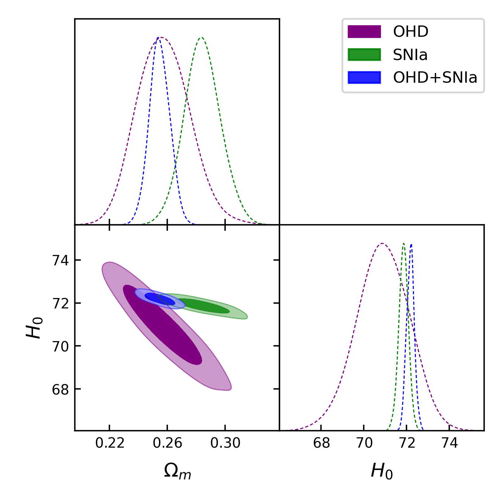
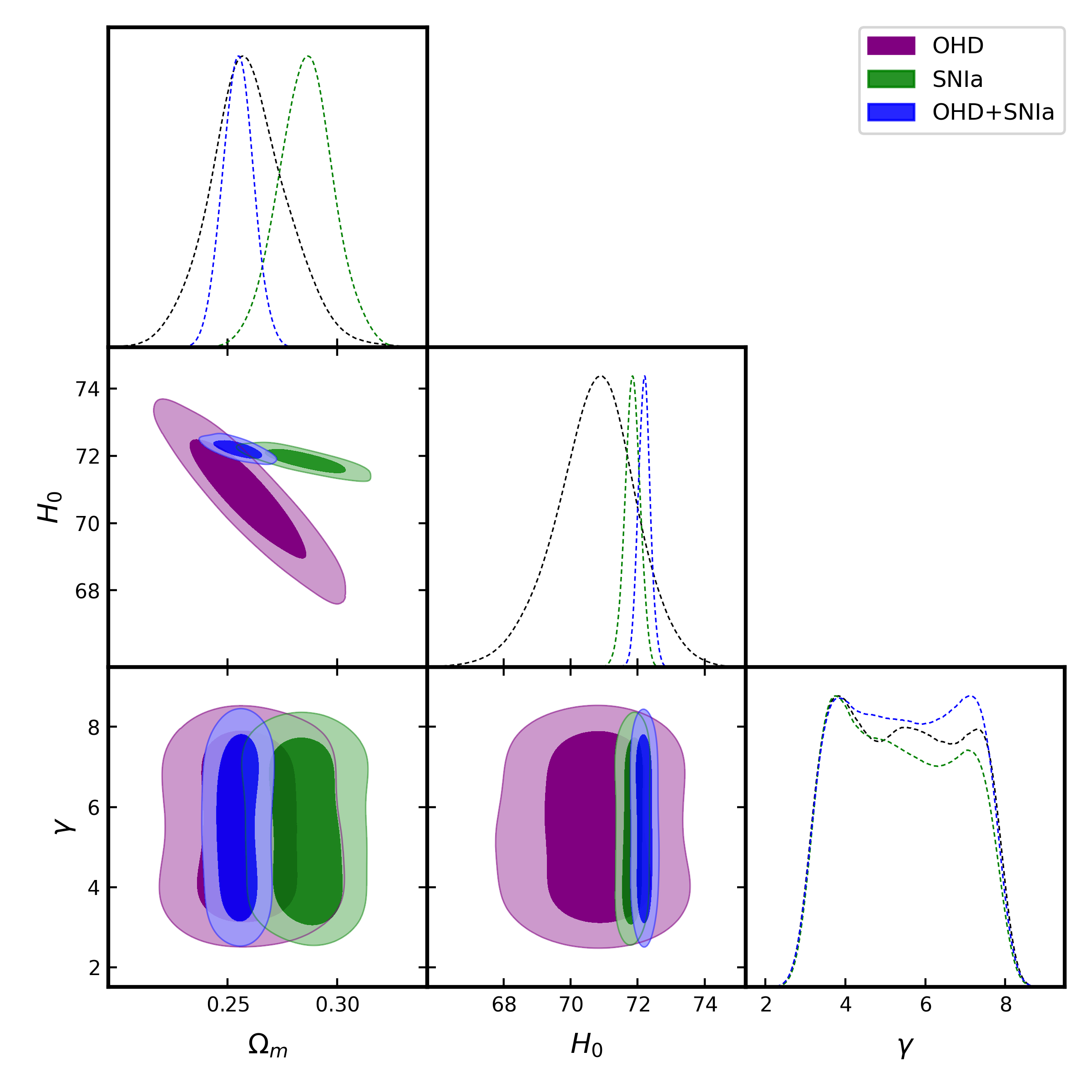
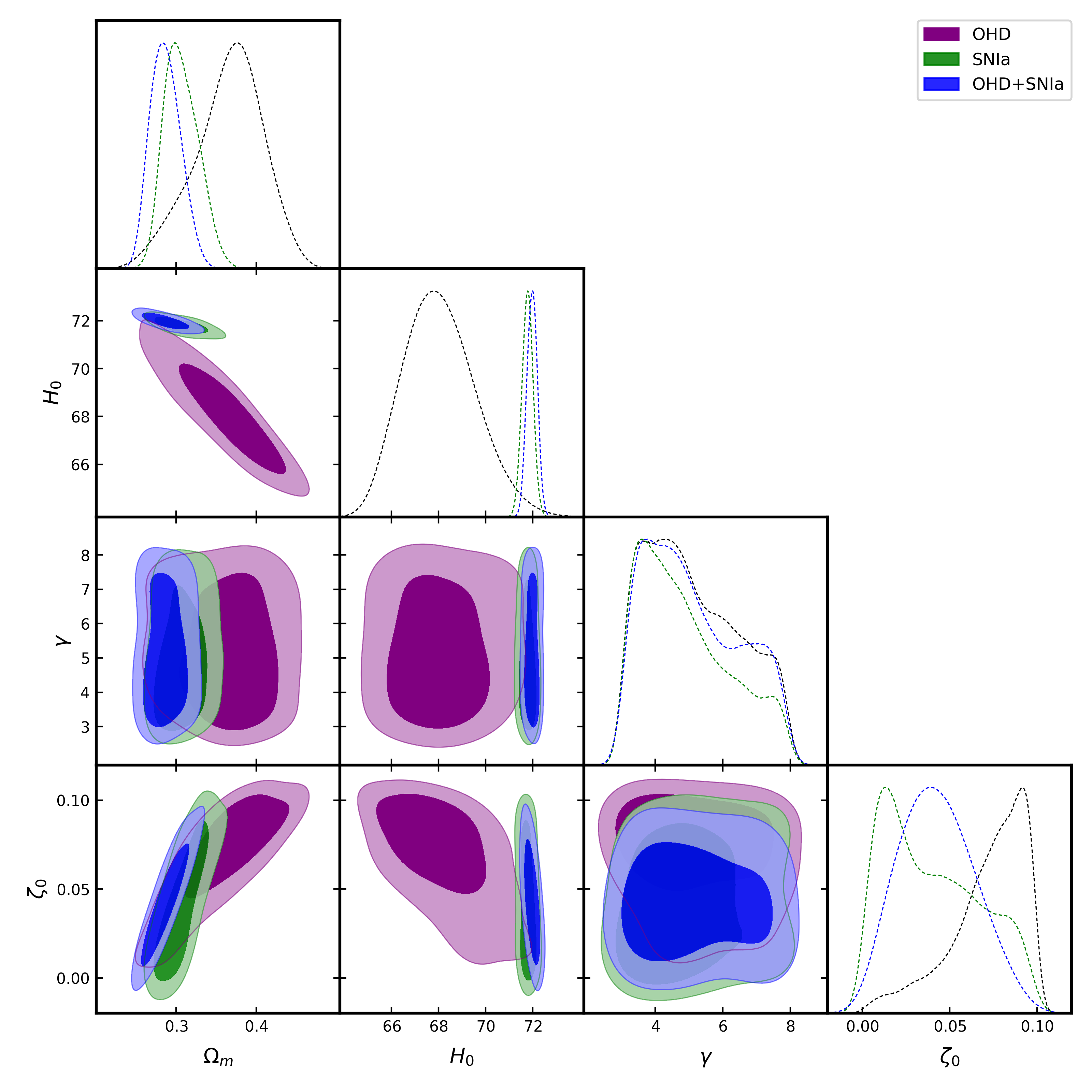
First, we focus on explaining the background history of the Universe with and without the effect of bulk viscosity. We use the OHD, SNIa, and a combined OHD+SNIa datasets to constrain the observational parameters {, , }, and the exponents {, , } for the three viable gravity models, by utilizing a modified MCMC simulation originally developed in Hough
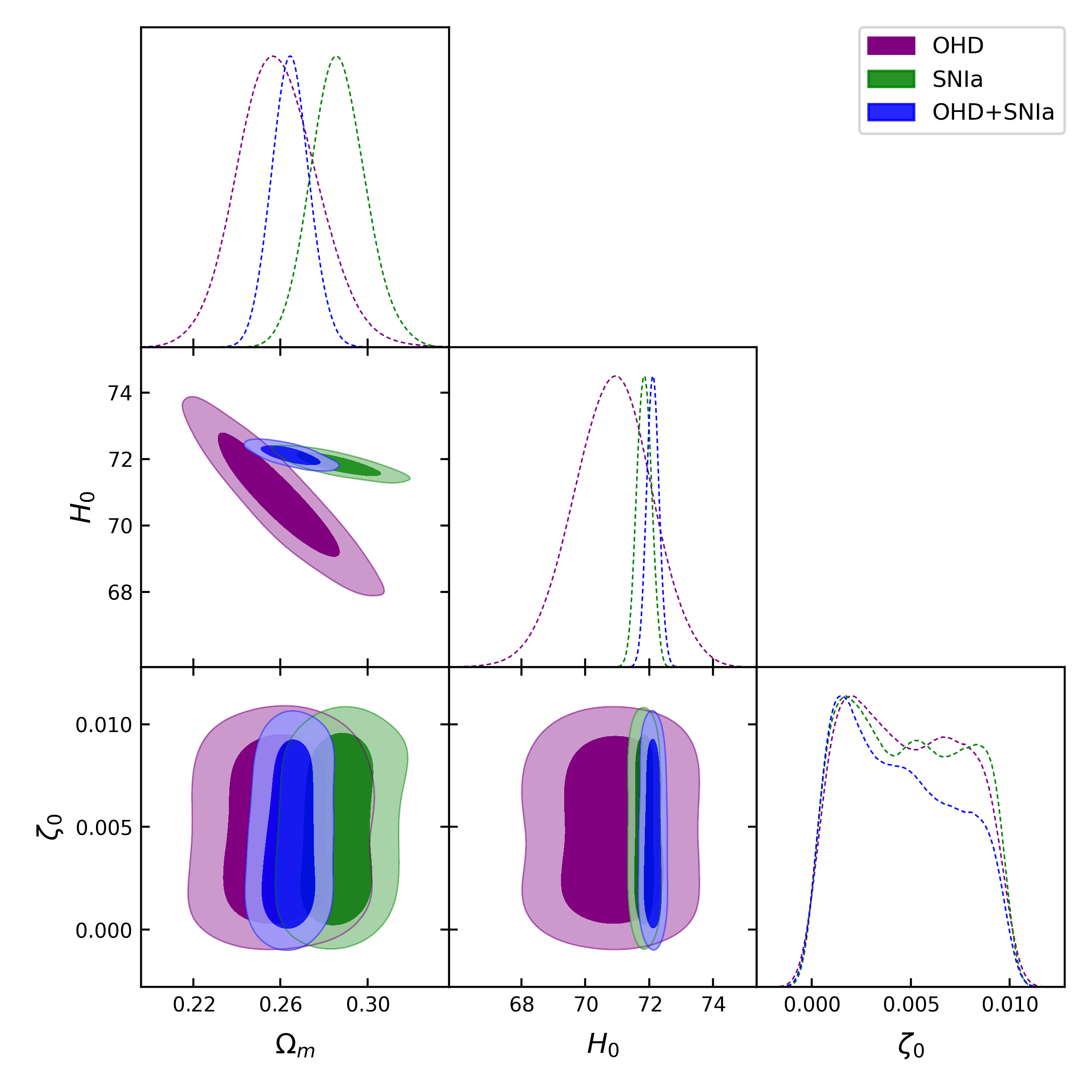
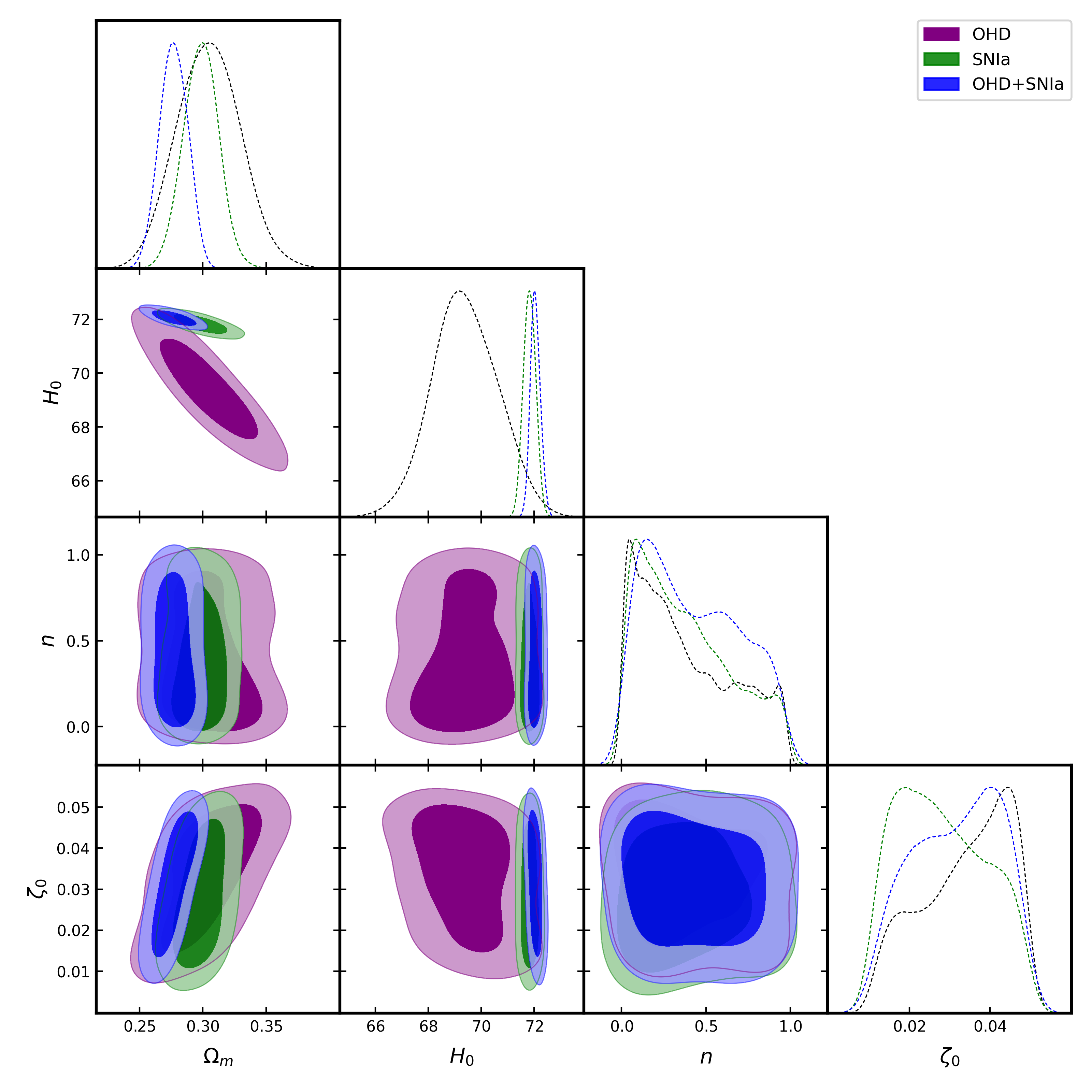
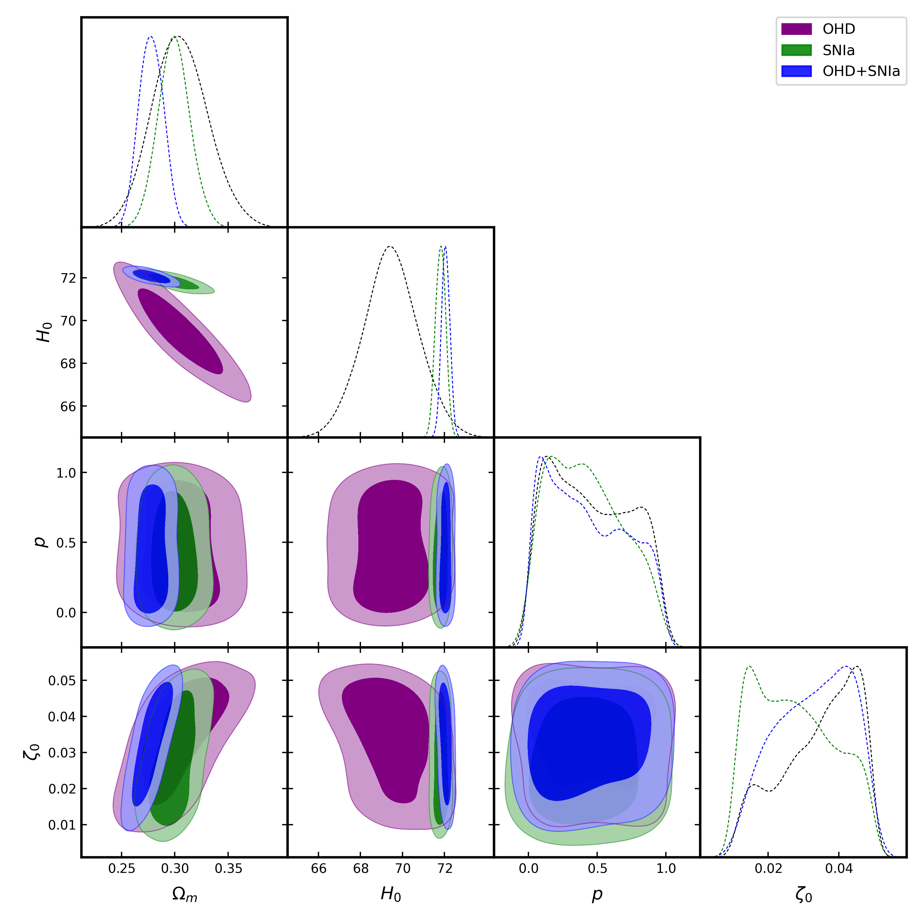
et al. (2020) to estimate the best-fit Gaussian distribution values of these the cosmological parameters which are crucial for understanding the Universe’s composition, structure, and evolution. Constraining these parameters also helps refine the gravity models of cosmic expansion and tests our theoretical predictions. This process reduces uncertainties, since accurate constraints improve the reliability of the cosmological conclusions and drive advances in both observational methods and theoretical physics. These calculated best-fit parameter values are presented in Tables 2 and 3 for both the CDM and gravity models for cases without and with the effect of bulk viscosity, respectively. The combined analysis of the results is presented in Fig. 1 for CDM and in Figs. 2, 3, and 4 for the gravity (, , and ) viable models, respectively at and confidence levels.
Furthermore, the statistically determined values for both models (CDM and gravity models) using OHD, SNIa and OHD+SNIa datasets has also been calculated. These include likelihood (), chi-square (), reduced chi-square (), Akaike Information Criterion (AIC), Change of AIC (), Bayesian Information Criterion (BIC) (Burnham &
Anderson, 2004), change of BIC (), the standard deviation () and the residues (). Since these statistical values are essential techniques in model selection, the goodness-of-fit compares the viability of the gravity models with that of CDM. For comparison purposes, we consider the CDM as the “accepted” model to justify the gravity model based on the AIC and BIC criteria. These criteria allow us to establish the acceptance or rejection of a particular gravity model. The AIC and BIC values are calculated using the following equations:
| (45) |
where is calculated using the model’s Gaussian likelihood function value and is the number of free parameters for the particular model. At the same time, is the number of data points for the dataset. We apply the Jeffreys scale (Nesseris & Garcia-Bellido, 2013) range to quantify whether a particular gravity model should be “accepted” or “rejected” compared to CDM. Accordingly, means that for the fitted data the proposed theoretical model holds a substantial observational support, means less observational support, and finally means no observational support.777N.B To avoid any confession, represents both and .
| Data | Model | ||||
| OHD | - | - | |||
| SNIa | - | - | |||
| OHD+SNIa | - | - | |||
| n | |||||
| OHD | - | ||||
| SNIa | - | ||||
| OHD+SNIa | - | ||||
| OHD | - | ||||
| SNIa | - | ||||
| OHD +SNIa | - | ||||
| OHD | - | ||||
| SNIa | - | ||||
| OHD +SNIa | - |
| Data | Model | ||||
| OHD | - | ||||
| SNIa | - | ||||
| OHD+SNIa | - | ||||
| OHD | |||||
| SNIa | |||||
| OHD+SNIa | |||||
| OHD | |||||
| SNIa | |||||
| OHD +SNIa | |||||
| OHD | |||||
| SNIa | |||||
| OHD +SNIa |
The statistics based information has been provided in Tables 4 and 5 for both with and without the bulk viscosity effects. Note that the discussions regarding the constraining statistical analysis for this work take into account the CMB based Aghanim et al. (2020) results: We assume the base CDM cosmology and the inferred (model-dependent) late-Universe parameter values for the Hubble constant km/s/Mpc; matter density parameter ; and matter fluctuation amplitude
| Data | AIC | BIC | |||||||||
|---|---|---|---|---|---|---|---|---|---|---|---|
| OHD | -16.23 | 32.46 | 0.58 | 36.46 | 0 | 40.54 | 0 | 10.413 | -2.264 | ||
| SNIa | -517.84 | 1035.68 | 0.99 | 1039.68 | 0 | 1049.59 | 0 | 0.143 | -0.006 | ||
| OHD+SNIa | -537.97 | 1075.94 | 0.98 | 1079.94 | 0 | 1091.30 | 0 | - | - | ||
| OHD | -14.25 | 28.5 | 0.51 | 34.50 | 1.96 | 40.63 | 0.09 | 10.425 | -1.676 | ||
| SNIa | -517.80 | 1035.6 | 0.98 | 1041.60 | 2.0 | 1056.46 | 6.87 | 0.142 | -0.001 | ||
| OHD+ SNIa | -537.97 | 1075.94 | 0.97 | 1081.94 | 2.00 | 1094.96 | 3.66 | - | - | ||
| OHD | -14.24 | 28.48 | 0.53 | 34.48 | 1.98 | 40.60 | 0.06 | 10.421 | -1.6767 | ||
| SNIa | -516.94 | 1032.8 | 0.98 | 1038.80 | 2.80 | 1053.66 | 4.07 | 0.145 | -0.005 | ||
| OHD+ SNIa | -537.60 | 1075.20 | 0.98 | 1081.20 | 1.30 | 1094.22 | 2.92 | - | - | ||
| OHD | -14.80 | 29.6 | 0.55 | 35.60 | 0.86 | 41.70 | 1.16 | 10.433 | -2.367 | ||
| SNIa | -517.32 | 1034.64 | 0.99 | 1040.64 | 0.96 | 1055.50 | 5.91 | 0.140 | -0.004 | ||
| OHD+ SNIa | -536.4 | 1072.8 | 0.97 | 1078.8 | 0.6 | 1093.82 | 2.52 | - | - |
| Data | AIC | BIC | ||||||||
|---|---|---|---|---|---|---|---|---|---|---|
| OHD | -14.08 | 28.17 | 0.587 | 34.17 | 0.0 | 39.975 | 0.0 | 10.379 | -1.522 | |
| SNIa | -517.91 | 1035.82 | 0.99 | 1041.82 | 0.0 | 1056.67 | 0.0 | 0.141 | -0.019 | |
| OHD+SNIa | -538.68 | 1077.36 | 0.98 | 1083.36 | 0.0 | 1098.36 | 0.0 | |||
| OHD | -13.55 | 27.11 | 0.57 | 35.11 | 0.94 | 42.84 | 2.86 | 10.197 | -1.558 | |
| SNIa | -517.9 | 1035.8 | 0.97 | 1045.8 | 3.98 | 1064.39 | 7.72 | 0.1472 | 0.007 | |
| OHD+ SNIa | -536.90 | 1073.80 | 0.98 | 1081.80 | 1.559 | 1101.81 | 3.45 | |||
| OHD | -13.33 | 26.66 | 0.56 | 34.66 | 0.49 | 42.38 | 2.40 | 10.1568 | -1.138 | |
| SNIa | -518.23 | 1036.46 | 0.99 | 1044.46 | 2.6 | 1064.28 | 7.60 | 0.144 | 0.005 | |
| OHD+ SNIa | -536.89 | 1073.78 | 0.98 | 1081.78 | 1.579 | 1101.79 | 3.43 | |||
| OHD | -12.90 | 25.81 | 0.549 | 33.81 | 0.35 | 41.53 | 1.55 | 10.089 | -1.461 | |
| SNIa | -518.97 | 1037.95 | 0.99 | 1045.95 | 4.13 | 1065.77 | 9.09 | 0.141 | -0.004 | |
| OHD+ SNIa | -538.33 | 1076.66 | 0.98 | 1084.66 | 1.30 | 1102.1 | 3.57 |
From the constraining of cosmic accelerating expansion and statistical best-fit analysis (Tables 2 - 5), we can determine the following properties of each of the three models. Firstly, without bulk viscosity, we note that our first model , has the highest constrained value on any dataset between the three models. This is even more problematic, since it adds to the Hubble tension while being constrained on a dataset (OHD+SNIa) designed to more accurately represent cosmic acceleration than OHD and SNIa only datasets. In terms of constraining the cosmological parameters performed the best in relaxing the Hubble tension by obtaining the lowest value in the OHD+SNIa dataset, while obtain the lowest constrained value (specifically OHD) on any dataset, but with a large error.
From a statistical analysis point of view, we found that the OHD dataset resulted, on average, in the best for the three models relative to the CDM model, especially for , but the models tend to underestimate the actual data, resulting in large negative values. Therefore, the models were successfully fitted to the data, but the best-fit results are not reliable. When looking at the SNIa dataset, both and are firmly in the category of less observational support. For the combined OHD+SNIa data, these models do receive some validation, with even receiving the lowest value at 2.52. However, due to the underestimation of the best-fitted models on the OHD data, the viability of these models should be weighed against the SNIa data. From this, it is clear that performed the best statistically, although it itself also received “less observational support” from the SNIa dataset.
When the bulk viscosity is included in the models, is, on average, slightly decreased (relaxing the Hubble tension), for the three models in the three datasets, especially for the OHD dataset that received values lower than km/s/Mpc. In this case, it can be argued that we should only use the OHD results, since it relaxed the Hubble tension the most when the bulk viscosity is included. However, due to the necessary statistical weighting towards SNIa, the slight decrease in is not a significant improvement. This is further confirmed through the statistical analysis, where we note that most of the values (except for on the OHD+SNIa dataset) are much higher. This is especially notable in the SNIa only dataset where the three models with bulk viscosity would be “rejected” as possible alternative models. Therefore, the addition of bulk viscosity does not appear to improve the fitting of these models. However, there are two caveats to this statement. The first would be that the addition of bulk viscosity substantially improves the values with all three models close to being within -error888The constrained values is within on all three datasets. from the Aghanim
et al. (2020) values on all three datasets. This is a definitive improvement, especially for the SNIa data, where the CDM model cannot match the CMB-based Aghanim
et al. (2020) results. The second caveat would be the apparent decrease in the underestimation of the OHD data, therefore improving the reliability of the use of this dataset.
From the above, we can conclude that the addition of bulk viscosity statistically negatively influences these gravity models when matching to the cosmic accelerated expansion measurements, but that future research can be done on why the parameter values and the apparent underestimation on the OHD data improved. Furthermore, seems to match the observational results of the accelerating expansion most consistently between the three models, while seems to fair the worst.
4.2 Structure growth
Secondly, we focus on the study of the evolution of the Universe’s structure growth in the context of the bulk viscosity associated with gravity. Bulk viscosity can affect the growth rate of cosmic structures by introducing additional damping in the evolution of density perturbations (Zimdahl, 1996). This influences the distribution and clustering of matter (Yang et al., 2019)
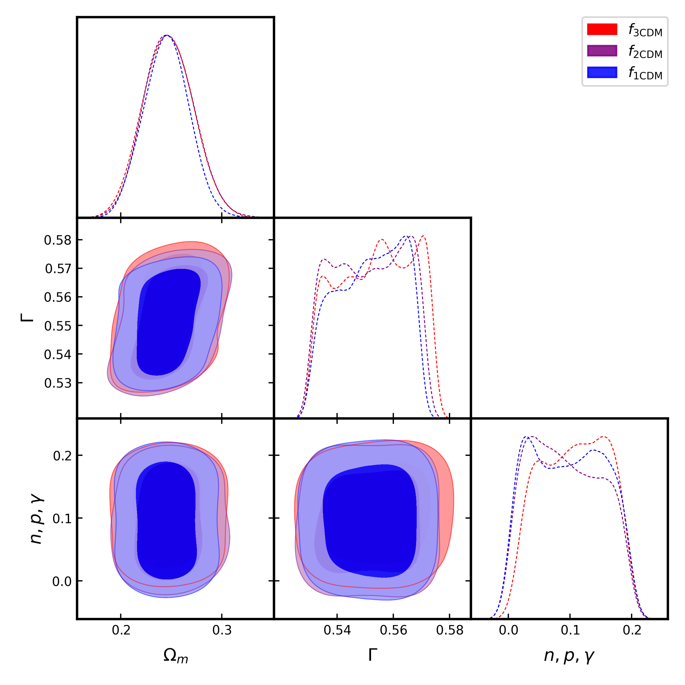
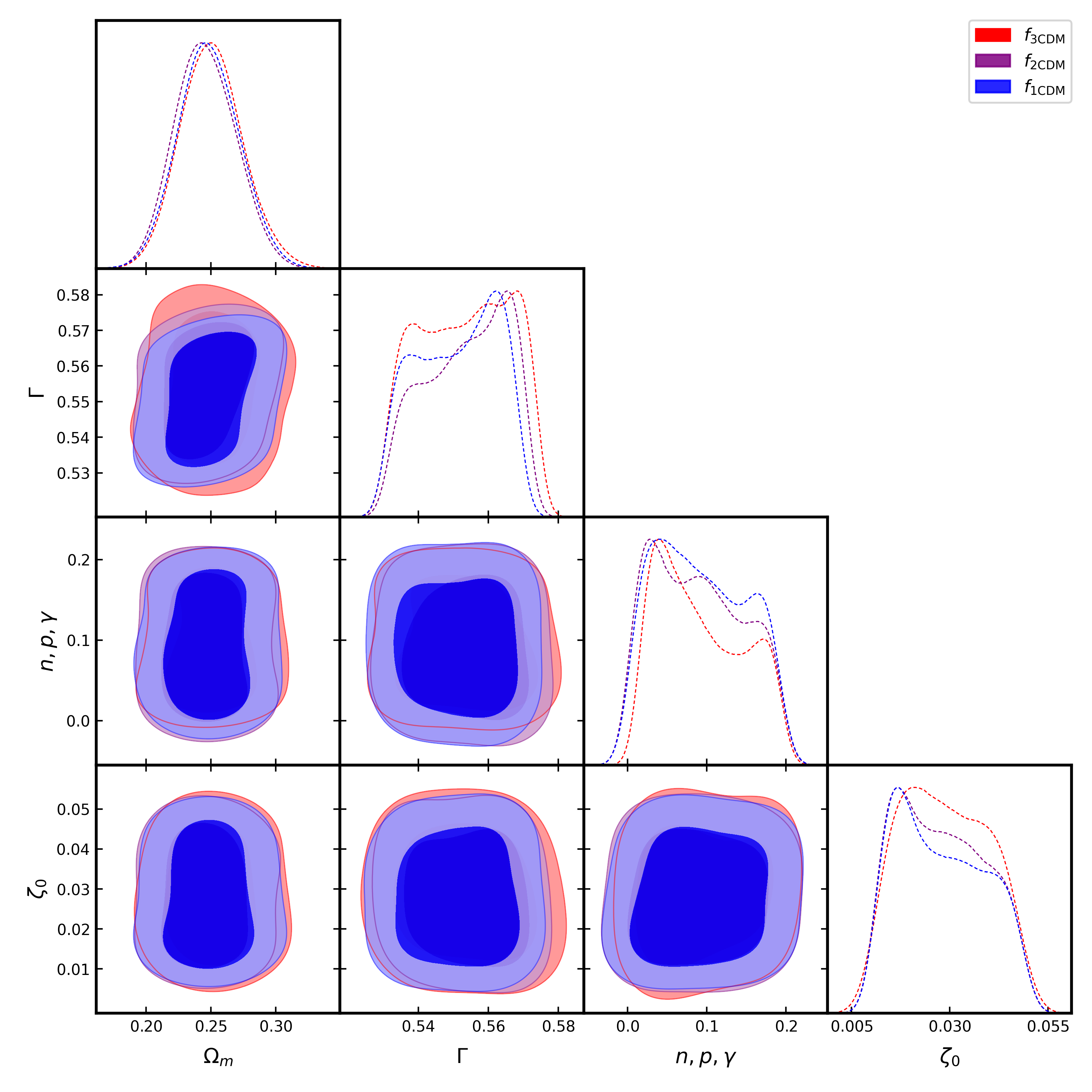
In this manuscript, we provide a detailed analysis of the contribution of gravity, both with and without the presence of bulk viscosity, to study the density contrast . This helps us to understand the formation of large-scale structures such as galaxies and clusters. We also present the growth factor , which describes the growth of density perturbations over time, and the growth rate , which provides information about how rapidly structures are forming and evolving. Furthermore, we discuss the redshift space distortion , which includes contributions from the peculiar velocities of galaxies as well as the Hubble flow. We have estimated values of the best-fit parameters {} and the model-free parameters using the same modified MCMC simulation (Hough
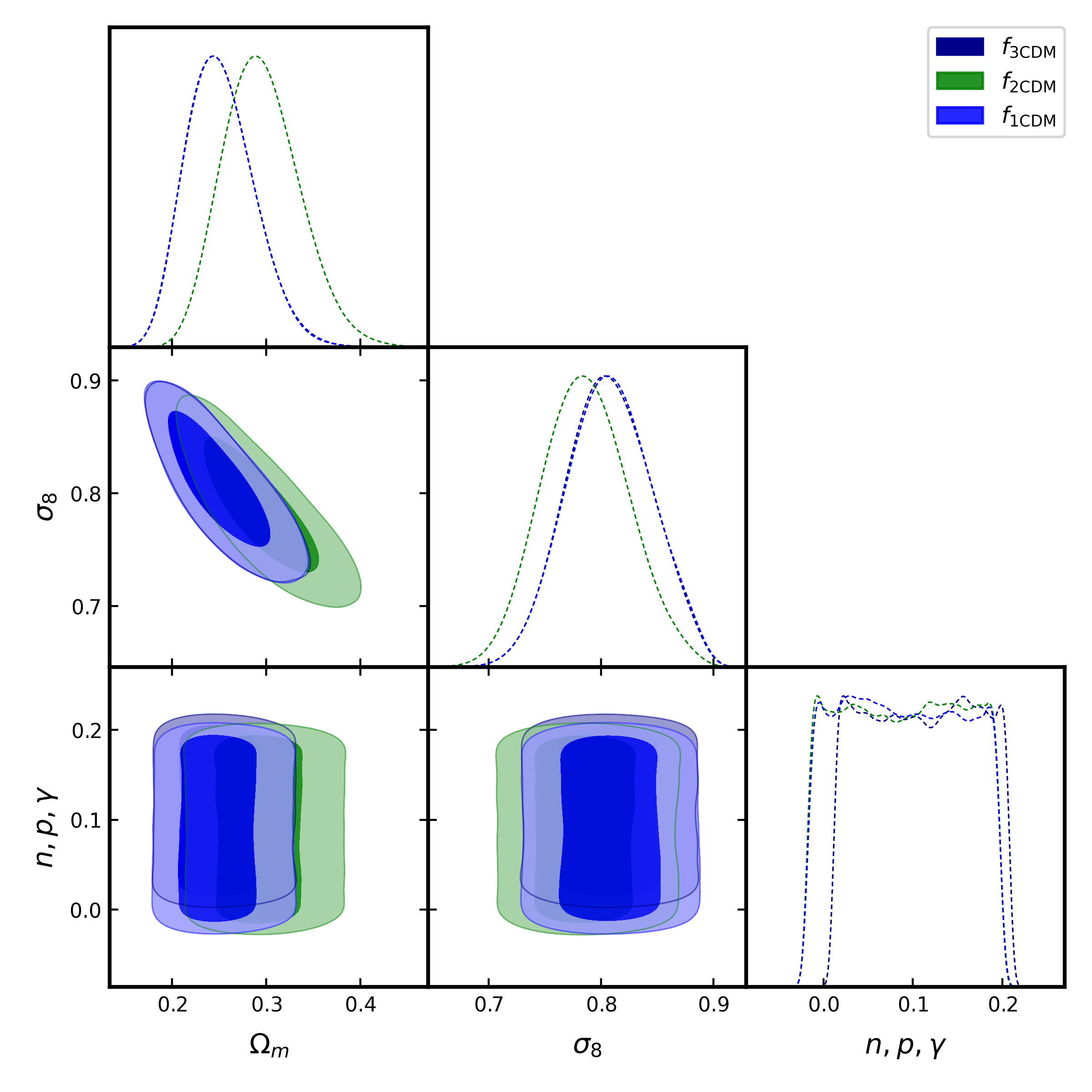
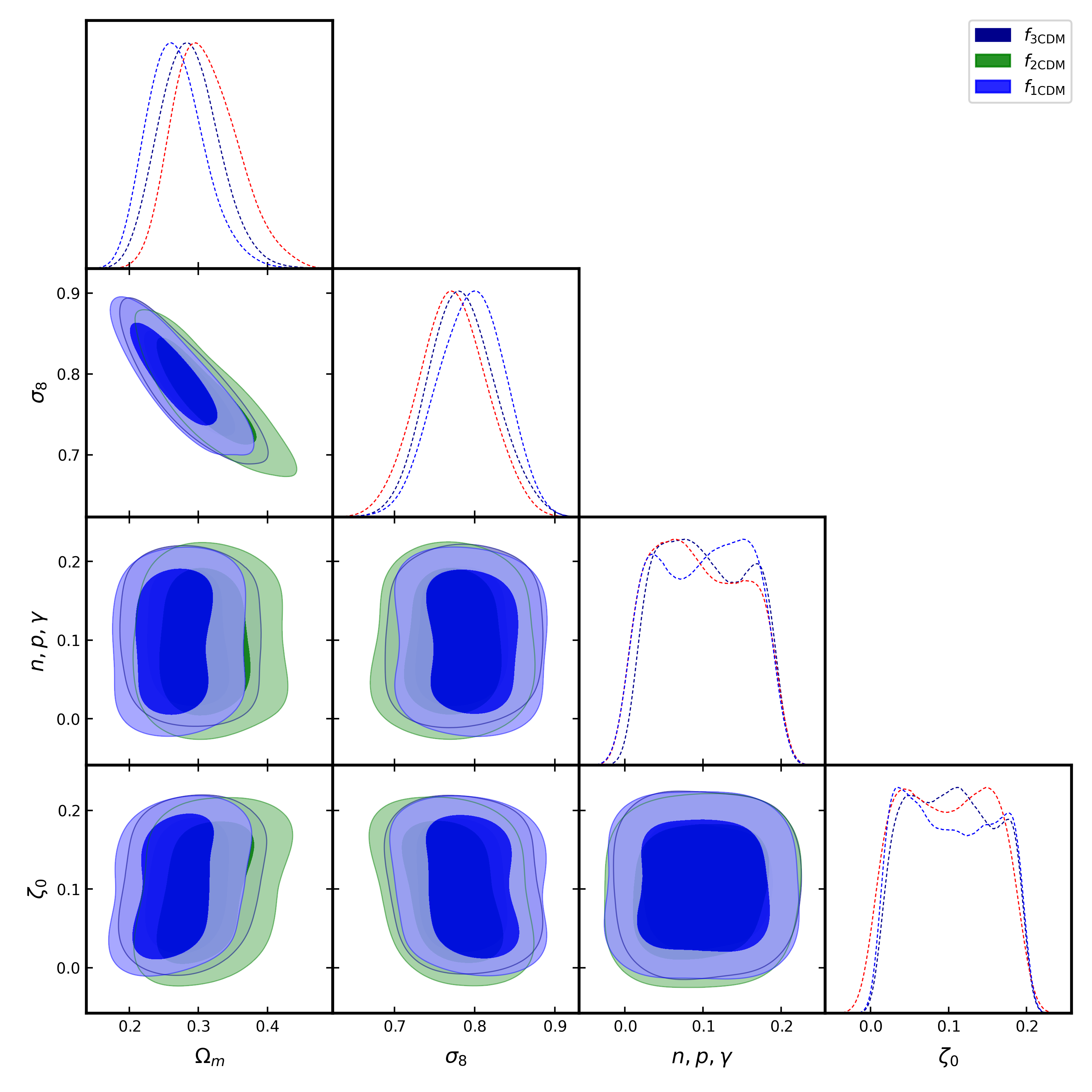
et al., 2020) for the large-scale structure datasets, f and f observations. The resulting contour plots are presented in Figs. 5 and 6, respectively, for the three models. In these figures, the right panels show the best-fit values of the model parameters without the effect of bulk viscosity, while the left panels show the impact of the bulk viscosity, which is consistent at and confidence levels.
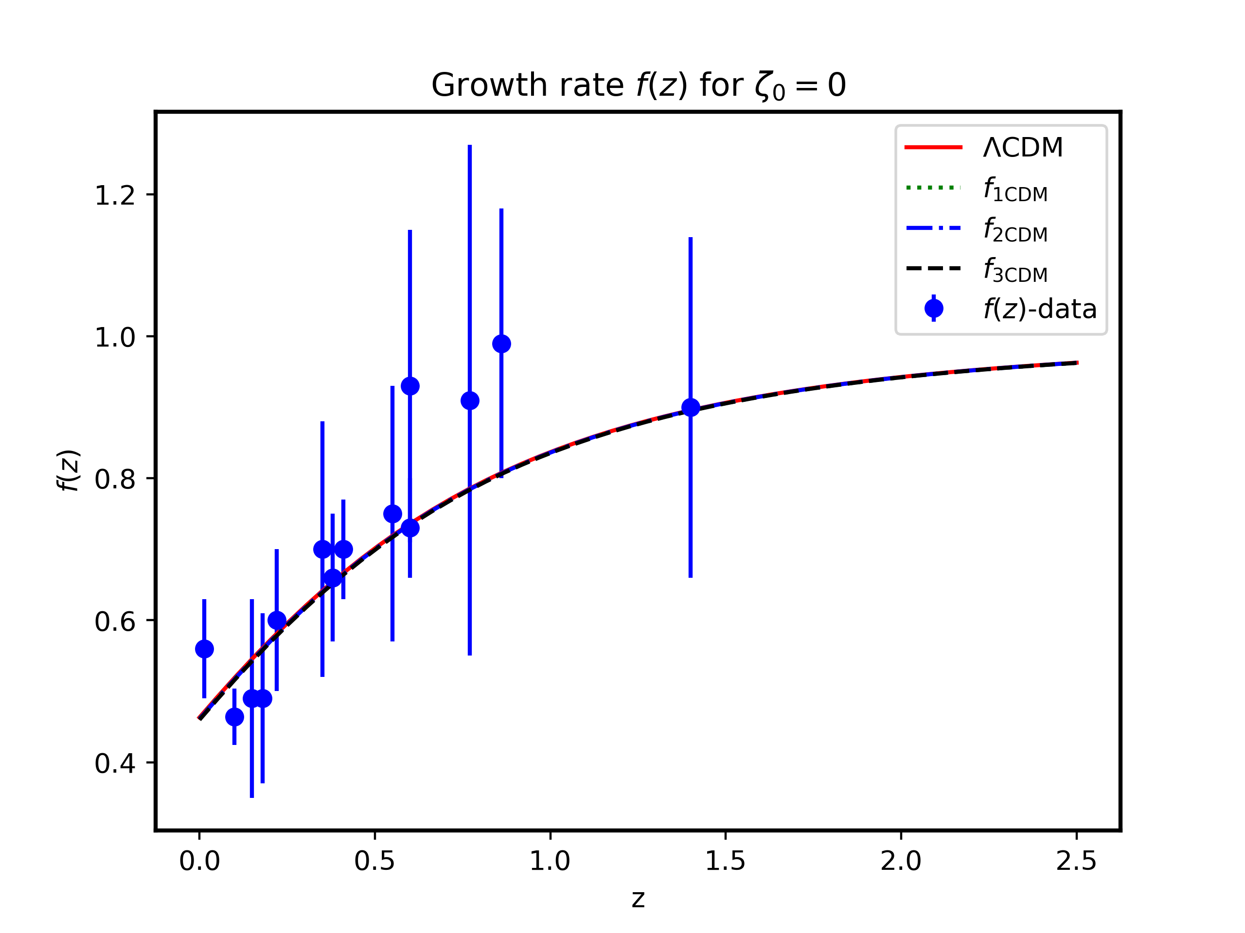
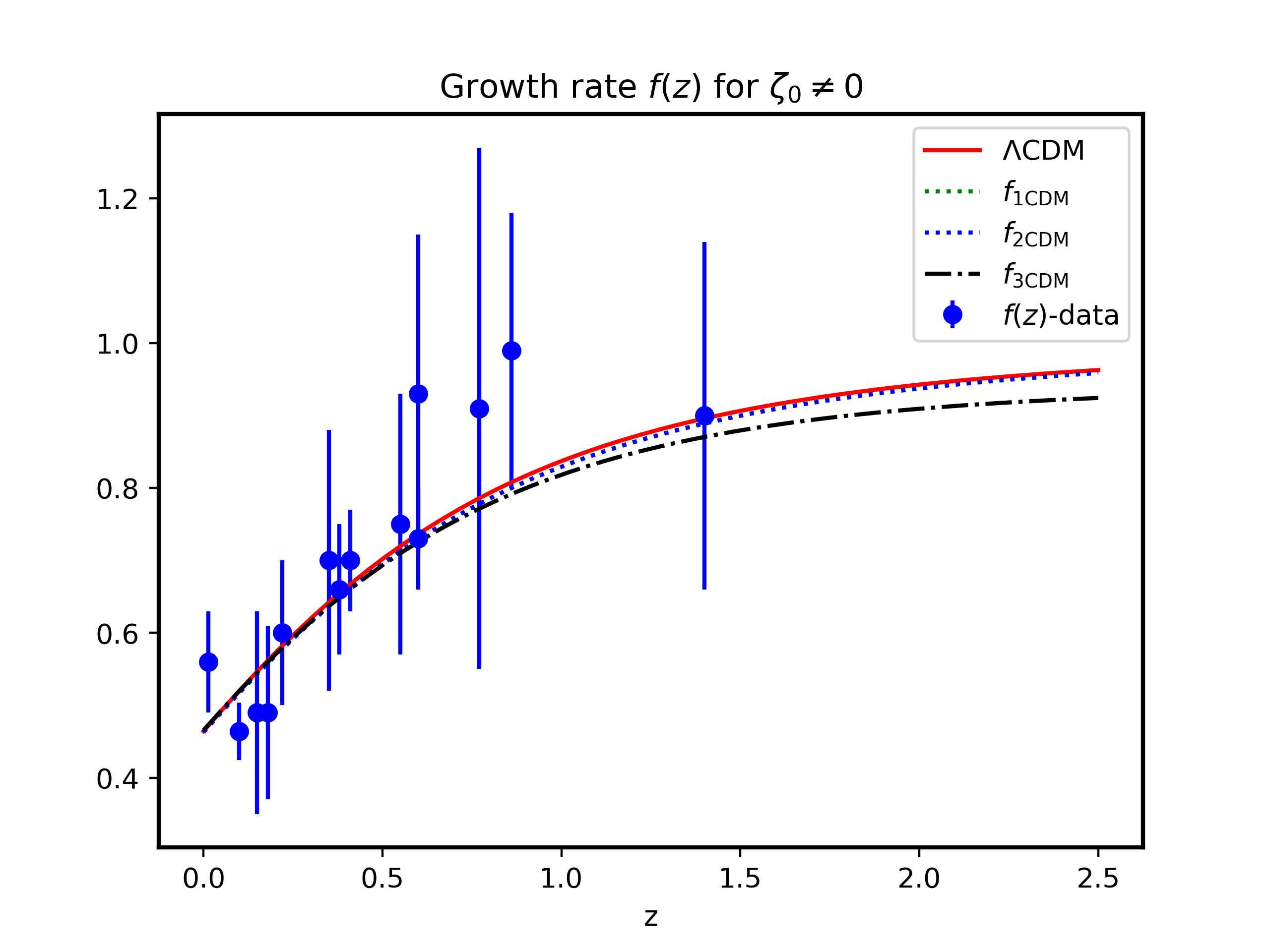
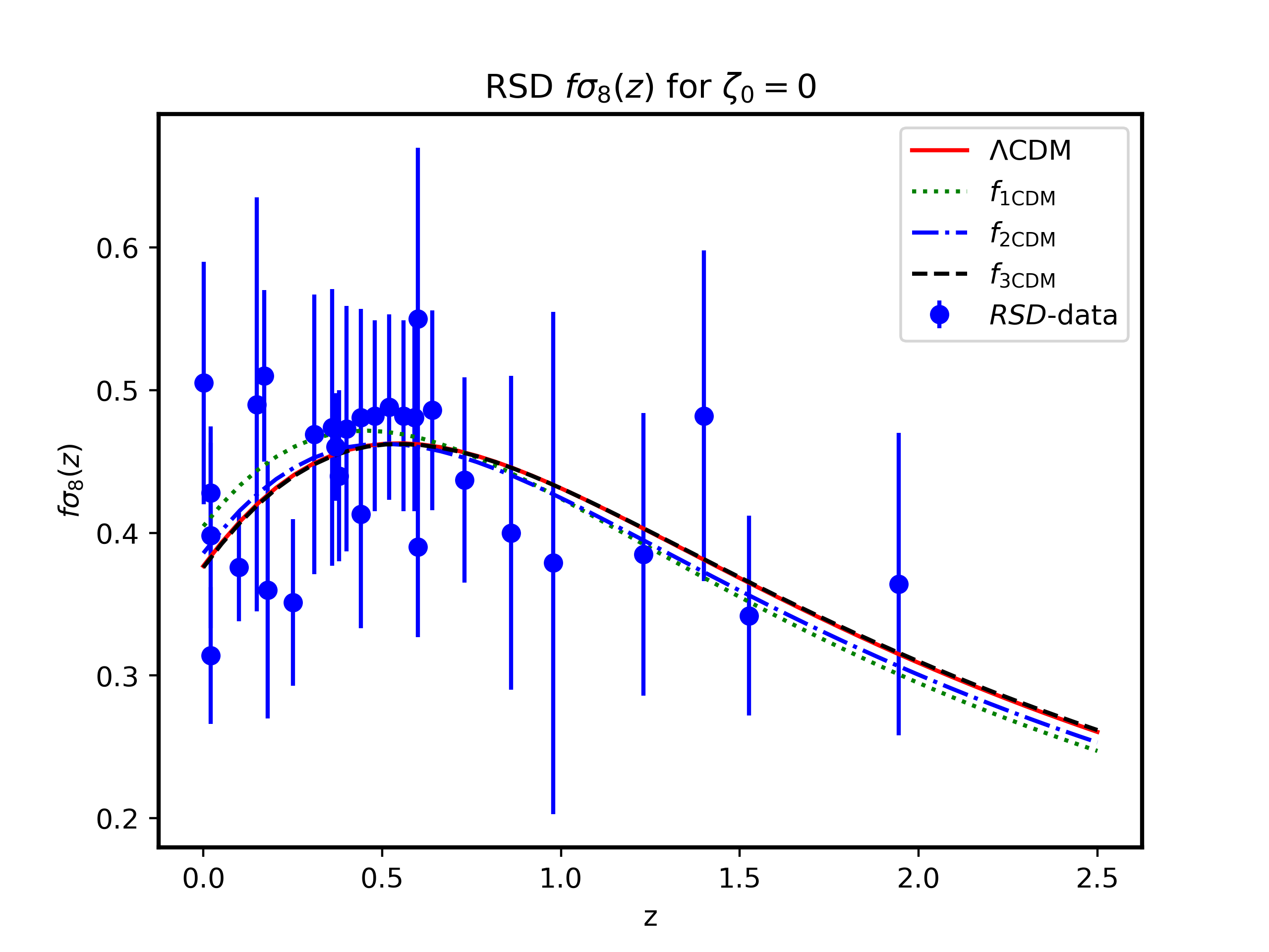
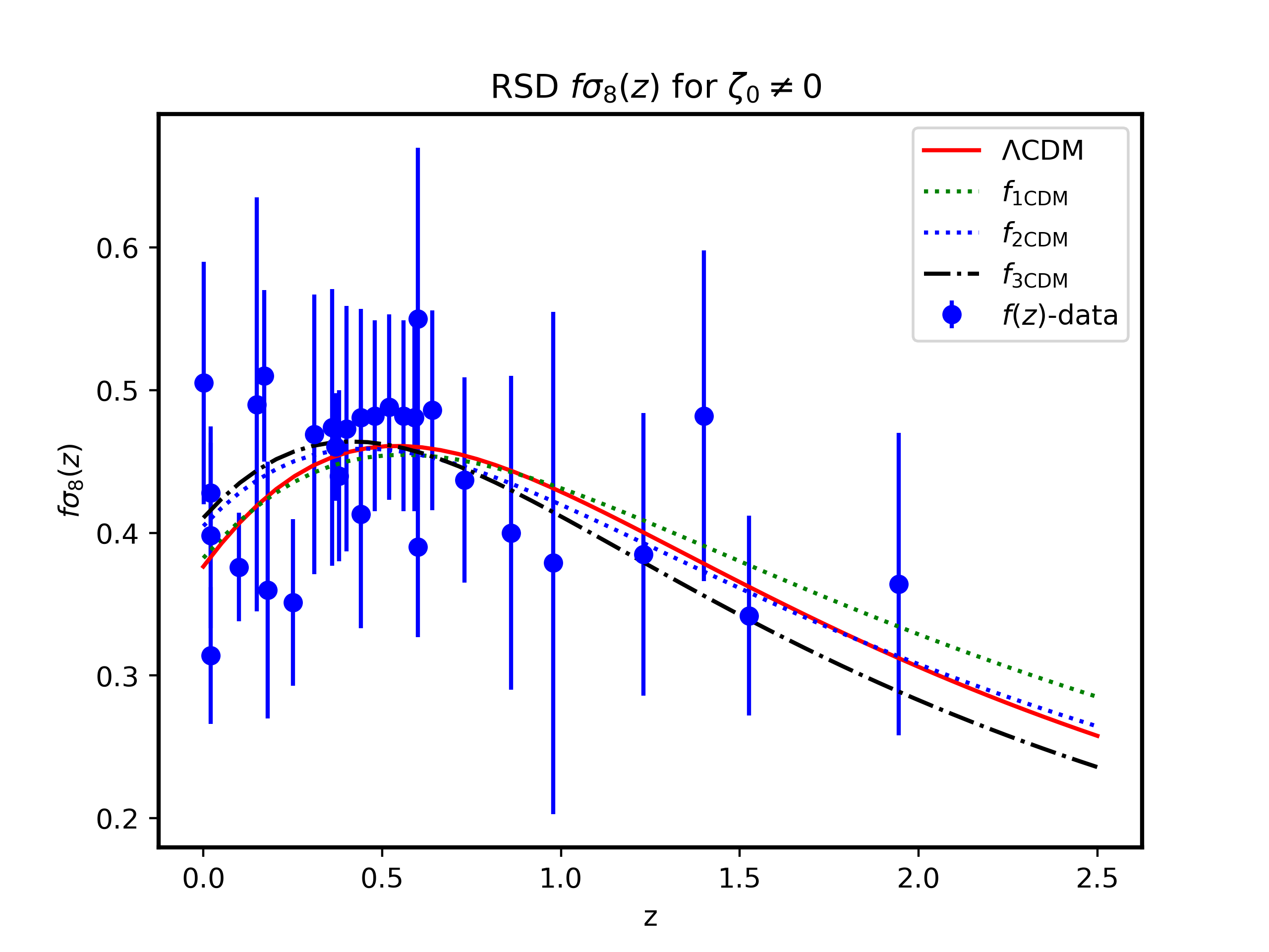
The best-fit values of these constraining parameters are presented in Tables 8 and 8 for both CDM and the three gravity models with and without the effect of bulk viscosity, respectively. We also provide numerical results of the growth factor as a function of cosmological redshift, without and with bulk viscosity effects. These results are displayed in Fig. 7, with the left panel showing the results without bulk viscosity and the right panel showing the results with bulk viscosity for the three different gravity models. Analysing these results allows us to measure how density perturbations evolve, eventually leading to the formation of cosmic structures such as galaxies and clusters of galaxies within the framework of the gravity model, both with and without the influence of bulk viscosity. From this plot, we observe that the gravity models without the bulk viscosity effect align more closely with the predictions of the CDM model. In the same manner, the redshift-space distortion as a function of the cosmological redshift is shown both without and with the effects of bulk viscosity in Fig. 8, in the top and right panels, respectively, for all three gravity models. From this diagram, we note that the theoretical predictions of all three gravity models align well with observational data from redshift-space distortions (f), compared to the CDM model, therefore visually increasing the validity of these models.
Statistical analysis has only been performed on the f and f datasets to further investigate the viability of these gravity models compared to the CDM model. These results are detailed in Tables 8 and 9. We computed the values of , , , AIC, , BIC, and for both the CDM model and the gravity models using the f and f datasets.
Based on the large-scale structure growth constraining and statistical best-fit analysis (Tables 8 - 9), we can determine the following properties of each of the three models. Firstly, for the f data, the three models obtained relatively close to the expected CDM model value (Linder &
Cahn, 2007) with and without bulk viscosity. However, all three models interestingly obtained a (even if only slightly higher), indicating that the gravity models predict a faster structure growth rate relative to the CDM model. obtained the “worst” best-fit value between the three models, but still within the error range. “Worst” is relative in this context since it only means that this model predicts the fastest structure growth rate, while obtained the slowest growth of the three gravity models. Furthermore, the best-fit values, both with and without bulk viscosity, seem to be problematic, since the values obtained are lower than the expected CMB-based Planck
Collaboration et al. (2020) or even SNe-based results.
From a statistical analysis point of view, all values obtained indicate that the models fit the f data with relatively the same precision, without real distinction. All models obtained or are very close to the “substantial observational support” relative to the CDM model. The only slight difference that we note is that all models overestimated the f data and that both with and without bulk viscosity seems to be slightly favoured by obtaining the best values.
Secondly, for the f dataset, we note that the best-performing model to this point, namely , is the weakest fitted model, and the without bulk viscosity model is the best in this case, by obtaining the closest match to the expected value (Aghanim
et al., 2020). Furthermore, we also note once again that the addition of bulk viscosity negatively influenced the models.
From a statistical point of view, the models still obtained a strong indication of observational support, but again show no real difference between the three models. Some minor notable statistical values obtained from the f dataset include that all models have only a very slight underestimation of the data, therefore taking most of the data into account. without bulk viscosity actually obtained the best and second best values even though it obtained the lowest values.
In conclusion, we cannot make a clear stance on the strength of each of the models on these two structure growth datasets, as they all received very similar results. None of them are rejected as viable models, but we did not learn any valuable property from them on the growth of large-scale structures. The only notable caveat would be the fact that once again the addition of bulk viscosity negatively affected these gravity models.
| For the case of | ||||
|---|---|---|---|---|
| Parameters | ||||
| - | - | |||
| - | ||||
| - | ||||
| - | ||||
| For the case of | ||||
| - | ||||
| For the case of | ||||
|---|---|---|---|---|
| Parameters | ||||
| - | - | |||
| - | ||||
| - | ||||
| - | ||||
| For the case of | ||||
| - | ||||
| Data | AIC | BIC | ||||||||
|---|---|---|---|---|---|---|---|---|---|---|
| f | -3.126 | 6.252 | 0.521 | 10.252 | 0.00 | 11.963 | 0.00 | 0.216 | 0.110 | |
| f | -8.00 | 16.00 | 0.57 | 20.00 | 0.00 | 24.00 | 0.00 | 0.084 | -0.058 | |
| f | -3.12 | 6.24 | 0.13 | 12.24 | 1.99 | 14.15 | 2.18 | 0.217 | 0.107 | |
| f | -7.69 | 15.38 | 0.59 | 21.38 | 1.58 | 25.58 | 1.58 | 0.092 | -0.060 | |
| f | -3.11 | 6.23 | 0.12 | 12.23 | 1.98 | 14.14 | 2.17 | 0.217 | 0.109 | |
| f | -7.78 | 15.56 | 0.57 | 21.56 | 1.55 | 25.77 | 1.76 | 0.086 | -0.061 | |
| f | -3.14 | 6.28 | 0.13 | 12.28 | 2.02 | 14.19 | 2.22 | 0.217 | 0.108 | |
| f | -7.80 | 15.61 | 0.57 | 21.61 | 1.60 | 25.82 | 1.82 | 0.083 | -0.057 |
| Data | AIC | BIC | ||||||||
|---|---|---|---|---|---|---|---|---|---|---|
| f | -3.5 | 7.0 | 0.61 | 13.0 | 0.0 | 41.91 | 0.0 | 0.215 | 0.116 | |
| f | -7.79 | 15.58 | 0.57 | 21.58 | 0.0 | 25.78 | 0.0 | 0.084 | -0.059 | |
| f | -3.03 | 6.07 | 0.13 | 14.07 | 1.07 | 16.62 | 1.71 | 0.215 | 0.106 | |
| f | -7.78 | 15.57 | 0.59 | 23.57 | 1.99 | 29.17 | 3.39 | 0.075 | -0.049 | |
| f | -2.97 | 5.94 | 0.13 | 13.94 | 1.94 | 16.50 | 0.12 | 0.216 | 0.103 | |
| f | -7.96 | 15.92 | 0.612 | 23.92 | 0.35 | 29.52 | 3.73 | 0.084 | -0.058 | |
| f | -3.04 | 6.09 | 0.13 | 14.09 | 1.09 | 16.55 | 1.64 | 0.210 | 0.090 | |
| f | -7.94 | 15.88 | 0.61 | 23.88 | 1.70 | 29.49 | 3.70 | 0.0942 | -0.0704 |
5 Conclusions
This work extensively analysed the late-time cosmic-accelerated expansion and the evolution and formation of large-scale structures, through the utilization of recent observational cosmological data. In particular, we studied these phenomena within the framework of gravity models, by probing the impact of the bulk viscosity. This study aimed to gauge the validity and broader implications of the gravity models, with a focus placed on the role of bulk viscosity in gravity.
The theoretical foundation of gravity was expanded in Sect. 2, wherein bulk viscosity was integrated into the effective pressure of the matter fluid, denoted as . In Sect. 2.1 we introduced three distinct classes of gravity models namely: (i) power-law, (ii) exponential, and (iii) logarithmic models (termed , , and , respectively) to assess their viability in different cosmological scenarios. The derived normalized Hubble parameter expressions for each model are presented in Eqs. (14), (17), and (20) and the distance modulus expressions Eq. (22) were instrumental in evaluating the validity of these -gravity models along with the CDM predictions when confronted with recent cosmic measurements: OHD, SNIa and the combined sets of these cosmological datasets, OHD+SNIa.
To investigate the growth of structure in a viscous fluid, the theoretical framework of density contrast was detailed in Sect. 2.4 within the 1+3 covariant formalism. This section presented the evolution equations for scalar perturbations, incorporating spatial gradients of matter, volume expansion, and gauge-invariant variables defining the fluctuations of the energy density and momentum terms of the non-metricity treated as an extra “fluid", as outlined in Eq. (25) and (26). Implementing scalar- and harmonic-decomposition techniques and the second-order differential equations for the density contrast are derived: Eq. (33) for , Eq. (34) for , and Eq. (35) for . Additionally, the growth factor , growth rate , and are formulated in the context of the gravity model to understand the formation and evolution of large-scale structures in the Universe. These quantities are instrumental in testing the viability of the gravity theory and constraining parameters of cosmological models through observational data, which provided crucial insights into the Universe’s evolution from early epochs to late time.
In Sect. 4, extensive analysis has been conducted on constraining cosmological parameters utilizing MCMC simulations on various observational datasets. The corresponding statistical analysis was presented to quantify the viability of the gravity models. The included cosmic measurements datasets are: (i) OHD, (ii) SNIa, (iii) OHD+SNIa, and large-scale structure measurements (iv) f and (v) f. The best-fitting analysis was done on each dataset, both with and without the effects of bulk viscosity. To accomplish this, firstly, we constrained the parameters {, }, and the constants , with the addition of the coefficient of bulk viscosity values as depicted in the compacted form in Figs. 1 for the CDM model, and in Figs. 2, 3, and 4 for the , , and models, respectively, at and confidence levels using OHD, SNIa, OHD+SNIa datasets. We also provided these best-fit parameter values for each cosmological model, both with and without the effect of bulk viscosity, in Tables 2 and 3 for both CDM and gravity models. These parameter values are used to derive statistical metrics such as , , , AIC, , BIC, and presented in Tables 4 and 5 to justify our validity of our models being alternative gravity models relative to the CDM model.
From these constrained parameter values and statistical results we noted, that for the cosmic accelerating measurements, without bulk viscosity resulted in the most plausible alternative model relative to the CDM model by obtaining the lowest result by a significant margin. According to Jeffery’s scale for the SNIa only dataset, this model barely missed out on the substantial observational support category. However, this may seem incorrect seeing that did in fact obtain the lowest and for the combined OHD+SNIa data, which would make it the most plausible. However, we noted that all the models substantially underestimated the OHD data, therefore, we had to weight the statistical analysis towards the SNIa data. This gave the advantage. Furthermore, we also noted that the addition of bulk viscosity statically negatively impacted the models, with all three models receiving higher and values, indicating that there is “less observational support” for these models to be alternative models to the CDM model. One caveat would be that with the addition of bulk viscosity, the difference between the cosmic measurement predictions for and the CMB based prediction was lowered even though the models themselves struggled more to explain the data. More research can be done on this.
Secondly, we constrained the best-fit values of the parameters together with the constants and using the f and f datasets presented in Table 8 and 8 respectively. The MCMC outcomes of these parameters are also presented in Figs. 5 and 6 for all three gravity models for the case of and using confidence levels and using the same datasets. Using these parameters mentioned above, we present the numerical results of the growth rate, is showed in Fig .7 and the redshift-space distortion diagram is shown in Fig. 8 through cosmological redshift with the corresponding datasets. We also used statistical analysis and presented the values of , , , AIC, , BIC, , and using the f and f datasets.
From our statistical results on large-scale structure growth, we noted from a statistical analysis point of view that there is no real difference between the three models, with being only slightly favoured. Furthermore, the three models were “accepted” as alternative models relative to the CDM model according to the and values. However, due to the similarities between all three models, for both the constraining of the parameters and the best-fit statistical analysis, we cannot make a distinction between each model’s individual properties and whether they are truly viable alternative models based on the f and data, since the cosmic measurements gave a different view. We once again determined that the addition of bulk viscosity negatively impacted the statistical viability of these models. Interestingly, we did note that for all three models, we found , therefore, indicating a faster structure growth rate than predicted by the CDM model, which requires further research.
Although testing against the observational datasets considered in this work has provided some insight into the acceptability of the three toy models in a viscous fluid medium, a similar analysis needs to be done using other types of data, such as those incorporating CMB and BAO physics, to put more stringent constraints on the cosmological viability of the models.
Data Availability
References
- Abebe et al. (2012) Abebe A., Abdelwahab M., De la Cruz-Dombriz A., Dunsby P. K., 2012, Classical and Quantum Gravity, 29, 135011
- Abebe et al. (2013) Abebe A., de la Cruz-Dombriz A., Dunsby P. K., 2013, Physical Review D, 88, 044050
- Acquaviva et al. (2016) Acquaviva G., John A., Pénin A., 2016, Physical Review D, 94, 043517
- Aghanim et al. (2020) Aghanim N., et al., 2020, Astronomy & Astrophysics, 641, A6
- Avila et al. (2021) Avila F., Bernui A., de Carvalho E., Novaes C. P., 2021, Monthly Notices of the Royal Astronomical Society, 505, 3404
- Avila et al. (2022) Avila F., Bernui A., Bonilla A., Nunes R. C., 2022, The European Physical Journal C, 82, 594
- Blake et al. (2011) Blake C., et al., 2011, Monthly Notices of the Royal Astronomical Society, 415, 2876
- Blake et al. (2012) Blake C., et al., 2012, Monthly Notices of the Royal Astronomical Society, 425, 405
- Blake et al. (2013) Blake C., et al., 2013, Monthly Notices of the Royal Astronomical Society, 436, 3089
- Blas et al. (2015) Blas D., Floerchinger S., Garny M., Tetradis N., Wiedemann U. A., 2015, Journal of Cosmology and Astroparticle Physics, 2015, 049
- Boyanovsky et al. (2006) Boyanovsky D., De Vega H., Schwarz D., 2006, Annu. Rev. Nucl. Part. Sci., 56, 441
- Burnham & Anderson (2004) Burnham K. P., Anderson D. R., 2004, Sociological Methods & Research, 33, 261
- Capozziello & Capriolo (2024) Capozziello S., Capriolo M., 2024, Physics of the Dark Universe, p. 101548
- Capozziello & Shokri (2022) Capozziello S., Shokri M., 2022, Physics of the Dark Universe, 37, 101113
- Castaneda et al. (2016) Castaneda C., et al., 2016, PhD thesis, Universitäts-und Landesbibliothek Bonn
- Chimento et al. (1997) Chimento L. P., Jakubi A. S., Méndez V., Maartens R., 1997, Classical and Quantum Gravity, 14, 3363
- Colistete Jr et al. (2007) Colistete Jr R., Fabris J., Tossa J., Zimdahl W., 2007, Physical Review D, 76, 103516
- DaÂngela et al. (2008) DaÂngela J., et al., 2008, Monthly Notices of the Royal Astronomical Society, 383, 565
- Das & Debnath (2024) Das K. P., Debnath U., 2024, The European Physical Journal C, 84, 513
- Das et al. (2024) Das S., Chattopadhyay S., Beesham A., 2024, Journal of Computational and Theoretical Transport, pp 1–11
- Davis et al. (2011) Davis M., Nusser A., Masters K. L., Springob C., Huchra J. P., Lemson G., 2011, Monthly Notices of the Royal Astronomical Society, 413, 2906
- De La Torre et al. (2017) De La Torre S., et al., 2017, Astronomy & Astrophysics, 608, A44
- Dixit et al. (2023) Dixit A., et al., 2023, Indian Journal of Physics, 97, 3695
- Dunsby (1991) Dunsby P. K., 1991, Classical and Quantum Gravity, 8, 1785
- Dunsby et al. (1992) Dunsby P., Bruni M., Ellis G., 1992, Astrophys. J, 395, 34
- D’Ambrosio et al. (2022) D’Ambrosio F., Fell S. D., Heisenberg L., Kuhn S., 2022, Physical Review D, 105, 024042
- Ellis & Bruni (1989) Ellis G. F., Bruni M., 1989, Physical Review D, 40, 1804
- Ferraris et al. (1982) Ferraris M., Francaviglia M., Reina C., 1982, General Relativity and gravitation, 14, 243
- Foreman-Mackey et al. (2013) Foreman-Mackey D., Hogg D. W., Lang D., Goodman J., 2013, Publications of the Astronomical Society of the Pacific, 125, 306
- Gadbail & Sahoo (2024) Gadbail G. N., Sahoo P., 2024, Chinese Journal of Physics, 89, 1754
- Gadbail et al. (2021) Gadbail G. N., Arora S., Sahoo P., 2021, The European Physical Journal C, 81, 1088
- Gagnon & Lesgourgues (2011) Gagnon J.-S., Lesgourgues J., 2011, Journal of Cosmology and Astroparticle Physics, 2011, 026
- Graves & Argrow (1999) Graves R. E., Argrow B. M., 1999, Journal of Thermophysics and Heat Transfer, 13, 337
- Guzzo et al. (2008) Guzzo L., et al., 2008, Nature, 451, 541
- Hamilton (1998) Hamilton A., 1998, The Evolving Universe: Selected Topics on Large-Scale Structure and on the Properties of Galaxies, pp 185–275
- Heisenberg (2024) Heisenberg L., 2024, Physics Reports, 1066, 1
- Hough et al. (2020) Hough R., Abebe A., Ferreira S., 2020, The European Physical Journal C, 80, 787
- Howlett et al. (2015) Howlett C., Ross A. J., Samushia L., Percival W. J., Manera M., 2015, Monthly Notices of the Royal Astronomical Society, 449, 848
- Howlett et al. (2017) Howlett C., et al., 2017, Monthly Notices of the Royal Astronomical Society, 471, 3135
- Hudson & Turnbull (2012) Hudson M. J., Turnbull S. J., 2012, The Astrophysical Journal Letters, 751, L30
- Huterer et al. (2017) Huterer D., Shafer D. L., Scolnic D. M., Schmidt F., 2017, Journal of Cosmology and Astroparticle Physics, 2017, 015
- Jiménez et al. (2018) Jiménez J. B., Heisenberg L., Koivisto T., 2018, Physical Review D, 98, 044048
- Khyllep et al. (2021) Khyllep W., Paliathanasis A., Dutta J., 2021, Physical Review D, 103, 103521
- Khyllep et al. (2023) Khyllep W., Dutta J., Saridakis E. N., Yesmakhanova K., 2023, Physical Review D, 107, 044022
- Koussour et al. (2022) Koussour M., Shekh S., Bennai M., 2022, Journal of High Energy Astrophysics, 35, 43
- Lewis (2019) Lewis A., 2019, arXiv preprint arXiv:1910.13970
- Li & Xu (2014) Li W., Xu L., 2014, The European Physical Journal C, 74, 1
- Linder & Cahn (2007) Linder E. V., Cahn R. N., 2007, Astroparticle Physics, 28, 481
- Maartens (1995) Maartens R., 1995, Classical and Quantum Gravity, 12, 1455
- Maartens & Triginer (1997) Maartens R., Triginer J., 1997, Physical Review D, 56, 4640
- Nesseris & Garcia-Bellido (2013) Nesseris S., Garcia-Bellido J., 2013, Journal of Cosmology and Astroparticle Physics, 2013, 036
- Ntahompagaze et al. (2018) Ntahompagaze J., Abebe A., Mbonye M., 2018, International Journal of Modern Physics D, 27, 1850033
- Ntahompagaze et al. (2020) Ntahompagaze J., Sahlu S., Abebe A., Mbonye M. R., 2020, International Journal of Modern Physics D, 29, 2050120
- Okumura et al. (2016) Okumura T., et al., 2016, Publications of the Astronomical Society of Japan, 68, 38
- Percival (2005) Percival W. J., 2005, Astronomy & Astrophysics, 443, 819
- Pezzotta et al. (2017) Pezzotta A., et al., 2017, Astronomy & Astrophysics, 604, A33
- Planck Collaboration et al. (2020) Planck Collaboration et al., 2020, A&A, 641, A7
- Rana et al. (2024) Rana D. S., Solanki R., Sahoo P., 2024, Physics of the Dark Universe, 43, 101421
- Ross et al. (2007) Ross N. P., et al., 2007, Monthly Notices of the Royal Astronomical Society, 381, 573
- Sahlu et al. (2020) Sahlu S., Ntahompagaze J., Abebe A., de la Cruz-Dombriz Á., Mota D. F., 2020, The European Physical Journal C, 80, 422
- Sahlu et al. (2024) Sahlu S., de la Cruz-Dombriz Á., Abebe A., 2024, arXiv preprint arXiv:2405.07361
- Sami et al. (2021) Sami H., Sahlu S., Abebe A., Dunsby P. K., 2021, The European Physical Journal C, 81, 1
- Samushia et al. (2012) Samushia L., Percival W. J., Raccanelli A., 2012, Monthly Notices of the Royal Astronomical Society, 420, 2102
- Scolnic et al. (2018) Scolnic D. M., et al., 2018, The Astrophysical Journal, 859, 101
- Shekh et al. (2023) Shekh S., Bouali A., Mustafa G., Pradhan A., Javed F., 2023, Classical and Quantum Gravity, 40, 055011
- Shi (2019) Shi F., 2019, The Bulletin of The Korean Astronomical Society, 44, 78
- da Silva & Silva (2021) da Silva W., Silva R., 2021, The European Physical Journal C, 81, 403
- Singh (2008) Singh C., 2008, Pramana, 71, 33
- Song & Percival (2009) Song Y.-S., Percival W. J., 2009, Journal of Cosmology and Astroparticle Physics, 2009, 004
- Springel et al. (2006) Springel V., Frenk C. S., White S. D., 2006, nature, 440, 1137
- Tegmark et al. (2006) Tegmark M., et al., 2006, Physical Review D, 74, 123507
- Turnbull et al. (2012) Turnbull S. J., Hudson M. J., Feldman H. A., Hicken M., Kirshner R. P., Watkins R., 2012, Monthly Notices of the Royal Astronomical Society, 420, 447
- Wang et al. (2018a) Wang D., et al., 2018a, Monthly Notices of the Royal Astronomical Society, 477, 1528
- Wang et al. (2018b) Wang Y., Zhao G.-B., Chuang C.-H., Pellejero-Ibanez M., Zhao C., Kitaura F.-S., Rodriguez-Torres S., 2018b, Monthly Notices of the Royal Astronomical Society, 481, 3160
- Wilson et al. (2007) Wilson J. R., Mathews G. J., Fuller G. M., 2007, Physical Review D, 75, 043521
- Yang et al. (2019) Yang W., Pan S., Di Valentino E., Paliathanasis A., Lu J., 2019, Physical Review D, 100, 103518
- Yu et al. (2018) Yu H., Ratra B., Wang F.-Y., 2018, The Astrophysical Journal, 856, 3
- Zimdahl (1996) Zimdahl W., 1996, Physical Review D, 53, 5483