A nonparametric test for diurnal variation
in spot correlation processes

Abstract

The association between log-price increments of exchange-traded equities, as measured by their spot correlation estimated from high-frequency data, exhibits a pronounced upward-sloping and almost piecewise linear relationship at the intraday horizon. There is notably lower—on average less positive—correlation in the morning than in the afternoon. We develop a nonparametric testing procedure to detect such deterministic variation in a correlation process. The test statistic has a known distribution under the null hypothesis, whereas it diverges under the alternative. It is robust against stochastic correlation. We run a Monte Carlo simulation to discover the finite sample properties of the test statistic, which are close to the large sample predictions, even for small sample sizes and realistic levels of diurnal variation. In an application, we implement the test on a monthly basis for a high-frequency dataset covering the stock market over an extended period. The test leads to rejection of the null most of the time. This suggests diurnal variation in the correlation process is a nontrivial effect in practice.

JEL Classification: C10; C80.

Keywords: diurnal variation; functional central limit theorem; high-frequency data; spot correlation; time-varying covariance.

1 Introduction

Correlation percolates through financial economics. It is a critical ingredient in the determination of optimal portfolio weights in a Markowitz (1952) mean-variance asset allocation problem, where the asset return correlations also determine a lower bound on diversification. Moreover, the correlation between the return of an asset and the return of the market portfolio is paramount in single- and multi-factor capital asset pricing models (Fama and French, 2015; Sharpe, 1964), where it is used to calculate the so-called beta, which is an important driver of the premium over the risk free rate earned as a compensation by investing in the risky asset. In addition, correlation is also employed in risk management and hedging.

It has long been recognized that correlations are time-varying, and the vast majority of parametric models to describe interday correlation allow it to change dynamically (e.g. Engle, 2002; Noureldin, Shephard, and Sheppard, 2012). The properties of the correlation process has also been traversed in detail with nonparametric analysis from high-frequency data. This is typically done by studying a realized measure of the daily integrated covariance, which is mapped into a correlation estimate, e.g. Aït-Sahalia, Fan, and Xiu (2010) and Boudt, Cornelissen, and Croux (2012).

Surprisingly, relatively little is known about the behavior of correlation at the intraday horizon. This stands in sharp contrast to the volatility of individual equity returns that is known to evolve as a U- or reverse J-shaped curve with notably higher volatility near the opening and closing of the stock exchange than around noon (e.g., Harris, 1986; Wood, McInish, and Ord, 1985). Several estimators of the intraday volatility curve has emerged over the years, e.g. Andersen and Bollerslev (1997, 1998) propose a parametric model for periodicity in volatility, whereas Boudt, Croux, and Laurent (2011) and Christensen, Hounyo, and Podolskij (2018) develop nonparametric jump- and microstructure noise-robust estimators from high-frequency that verify the existence of a pervasive structure in the intraday volatility.

The most common setup for describing the dynamic of spot volatility of an asset log-return at the interday and intraday horizon is a multiplicative time series model:

$$\sigma_{t}=\sigma_{sv,t}\sigma_{u,t},$$ (1)

where $\sigma_{sv,t}$ is a stationary process meant to capture stochastic volatility, whereas $\sigma_{u,t}$ is a deterministic component intended to capture diurnal variation and therefore assumed to be a constant time-of-day factor (i.e., $\sigma_{u,t}=\sigma_{u,t-1}$).

In a bivariate setting, any systematic evolution in the volatility is automatically transferred to the covariance process, $c_{t}^{XY}=\sigma_{t}^{X}\sigma_{t}^{Y}\rho_{t}$, where $\sigma_{t}^{X}$ and $\sigma_{t}^{Y}$ represent the spot volatility of asset $X$ and $Y$, whereas $\rho_{t}$ is their correlation. If the individual return variation of $X$ and $Y$ follows (1), the covariance inherits an “imputed” diurnal pattern:

$$c_{t}^{XY}=\underbrace{\sigma_{sv,t}^{X}\sigma_{sv,t}^{Y}}_{\text{stochastic volatility}}\times\underbrace{\rho_{t}}_{\text{spot correlation}}\times\underbrace{\sigma_{u,t}^{X}\sigma_{u,t}^{Y}}_{\text{imputed diurnal covariance}}.$$ (2)

However, observing (2) suggests that there may be an additional source of diurnal variation in the covariance, since the dynamic of the spot correlation further affects it. As in (1), we can capture a recurrent behavior in the spot correlation as follows:

$$\rho_{t}=\rho_{sc,t}\rho_{u,t},$$ (3)

where $\rho_{sc,t}$ and $\rho_{u,t}$ are interpreted as above. In the modified setting of (3), the breakdown of the covariance into its component parts is now given by

$$c_{t}^{XY}=\underbrace{\sigma_{sv,t}^{X}\sigma_{sv,t}^{Y}\rho_{sc,t}}_{\text{stochastic covariance}}\times\underbrace{\sigma_{u,t}^{X}\sigma_{u,t}^{Y}\rho_{u,t}}_{\text{actual diurnal covariance}}.$$ (4)

To the extent that correlations vary systematically within a day, we should expect the actual and imputed diurnal covariance curve to deviate (see, e.g., Bibinger, Hautsch, Malec, and Reiss, 2019, for initial evidence of this effect). To get a first impression of this, we begin with an inspection of Panel A in Figure 2 in our empirical application in Section 6, where we compare the average imputed and actual intraday covariance curve calculated pairwise for a cross-section of members from the Dow Jones Industrial Average and a proxy for the market portfolio of aggregate movements in the U.S. equity market over the sample period 2010–2023. We observe a striking discrepancy between the two, most notably in the early morning and late afternoon. This provides strong evidence of this effect in the high-frequency data. Looking at it in terms of the correlation process in Panel B of the figure, we locate a very significant upward-sloping intraday correlation curve, which increases monotonically during the trading session in an almost piecewise linear fashion. This is consistent with Allez and Bouchaud (2011) and concurrent work of Hansen and Luo (2023). There are large jumps in the correlation around the release of macroeconomic information, which corresponds to a large influx of systematic risk to the market.

In this paper, we construct a testing procedure to detect diurnal variation in a correlation process. It distills local estimates of the spot correlation, after the high-frequency return series has been devolatized to remove the effect of idiosyncratic volatility (both deterministic and stochastic), thus isolating the correlation process, while also controlling for potential price jump variation. If there are systematic changes in the spot correlation estimates, the test statistic grows large and rejects the null hypothesis of no diurnal variation. This is related to, but different from, previous work by Reiss, Todorov, and Tauchen (2015) for testing a constant beta. Overall, in our empirical high-frequency data, we implement the test statistic on a month-by-month basis and find that the proposed test statistic rejects the null hypothesis most of the times, thus confirming the circumstantial evidence from Figure 2.

To highlight the exploitation of predictable dynamics in the correlation, we adopt the standpoint of a trader who hedges a long exposure in single stocks via the market portfolio. We report a nontrivial effect by incorporating diurnal correlation into the risk management process, relative to ignoring it, yielding a drop in combined portfolio variance of about twenty percent. It also delivers a much more stable hedge ratio during the course of the trading day, helping to reduce transaction costs derived from warehousing the risk.

The roadmap of the paper is as follows. In Section 2, we present the model and list the assumptions required to extract an intraday correlation curve from a bivariate time series of high-frequency data. In Section 3, we develop a standard point-in-time correlation estimator. In Section 4, we propose a testing procedure, which can be employed to uncover the existence of diurnal variation in correlation. We prove an asymptotic distribution theory both for a nonpivotal- and pivotal-based version of our test statistic. In Section 5, we inspect the small sample attributes of our framework via Monte Carlo simulation. In Section 6, we apply it to a large panel of equity data. In Section 7, we conclude. We relegate proofs to the Appendix.

2 Theoretical setup

We suppose a filtered probability space $(\Omega,\mathcal{F},(\mathcal{F}_{t})_{t\geq 0},P)$ describes a bivariate continuous-time log-price process $Z=(X,Y)^{\top}$, where $(\mathcal{F}_{t})_{t\geq 0}$ is a filtration and ^⊤ is the transpose operator. $Z$ is observed on $[0,T]$, where $T$ is the number of days in the sample and the subinterval $[t-1,t]$ is the $t$th day, for $t=1,\ldots,T$. We assume $Z$ is recorded discretely at the equidistant time points $t_{i}=t-1+i/n$, for $i=0,1,\ldots,n$, so a total of $nT$ increments are observed with an equidistant time gap of $\Delta=1/n$. Throughout, the asymptotic theory is infill and long-span, i.e. we look at limits in which the time gap between consecutive observations goes to zero ($\Delta\rightarrow 0$ or $n\rightarrow\infty$) and the sample period increases ($T\rightarrow\infty$).

In absence of arbitrage (or rather a free lunch with vanishing risk) $Z$ is a semimartingale (e.g., Delbaen and Schachermayer, 1994). We suppose $Z$ is of the Itô-type, which is a process with absolutely continuous components. Then, we can write the time $t$ value of $Z$ as follows:

$$Z_{t}=Z_{0}+\int_{0}^{t}a_{s}\mathrm{d}s+\int_{0}^{t}\sigma_{s}\mathrm{d}W_{s}+J_{t},\quad t\geq 0,$$ (5)

where $Z_{0}=(X_{0},Y_{0})^{\top}$ is $\mathcal{F}_{0}$-measurable,

$$a_{t}=\begin{bmatrix}a_{t}^{X}\\ a_{t}^{Y}\end{bmatrix},\quad\sigma_{t}=\begin{bmatrix}\sigma_{t}^{X}&0\\ \rho_{t}\sigma_{t}^{Y}&\sqrt{1-\rho_{t}^{2}}\sigma_{t}^{Y}\end{bmatrix},\quad W_{t}=\begin{bmatrix}W_{t}^{X}\\ W_{t}^{Y}\end{bmatrix},\quad\text{and }J_{t}=\begin{bmatrix}J_{t}^{X}\\ J_{t}^{Y}\end{bmatrix},$$ (6)

where $(a_{t})_{t\geq 0}$ is a predictable and locally bounded drift, $(\sigma_{t})_{t\geq 0}$ is an adapted, càdlàg volatility matrix, while $(W_{t})_{t\geq 0}$ is a bivariate standard Brownian motion with $\langle W^{X},W^{Y}\rangle_{t}=0$, where $\langle\cdot,\cdot\rangle$ denotes the predictable part of the quadratic covariation process.

$J_{t}$ is a pure-jump process, for which we impose the following restriction.

Assumption (J):     $J_{t}^{\bullet}$ is such that

$$J_{t}^{\bullet}=\int_{0}^{t}\int_{\mathbb{R}}x\mu^{\bullet}(\mathrm{d}s,\mathrm{d}x),$$ (7)

where $\mu^{\bullet}$ is an integer-valued random measure on $\mathbb{R}_{+}\times\mathbb{R}$ with compensator $\nu^{\bullet}(\mathrm{d}t,\mathrm{d}x)=\chi_{t}^{\bullet}\mathrm{d}t\otimes F^{\bullet}(\mathrm{d}x)$, $\chi_{t}^{\bullet}$ is an adapted càdlàg process, and $F^{\bullet}$ is a measure on $\mathbb{R}$.

We also assume that the stochastic volatility processes are Itô semimartingale.

Assumption (V):     $\sigma_{t}^{\bullet}$ is of the form:

$$\begin{split}\sigma_{t}^{\bullet}&=\sigma_{0}^{\bullet}+\int_{0}^{t}\tilde{a}_{s}^{\bullet}\mathrm{d}s+\int_{0}^{t}\tilde{\sigma}_{s}^{\bullet}\mathrm{d}W_{s}+\int_{0}^{t}\tilde{\nu}_{s}^{\bullet}\mathrm{d}\tilde{W}_{s}+\int_{0}^{t}\int_{\mathbb{R}}x\tilde{\mu}^{\bullet}(\mathrm{d}s,\mathrm{d}x),\end{split}$$ (8)

where $(\tilde{a}_{t}^{\bullet})_{t\geq 0}$, $(\tilde{\sigma}_{t}^{\bullet})_{t\geq 0}$, $(\tilde{\nu}^{\bullet})_{t\geq 0}$, are adapted, càdlàg stochastic processes, $\tilde{W}_{t}=(\tilde{W}_{t}^{X},\tilde{W}_{t}^{Y})^{\top}$ is a bivariate standard Brownian motion, independent of $W$, but $\tilde{W}_{t}^{X}$ and $\tilde{W}_{t}^{Y}$ can be correlated. At last, $\tilde{\mu}^{\bullet}(\mathrm{d}t,\mathrm{d}x)$ is the counting jump measure of $\sigma_{t}^{\bullet}$ with compensator $\tilde{\chi}^{\bullet}_{t}\mathrm{d}t\otimes\tilde{F}^{\bullet}(\mathrm{d}x)$, where $\tilde{\chi}_{t}^{\bullet}$ is an adapted càdlàg process, and $\tilde{F}^{\bullet}$ is a measure on $\mathbb{R}$.

The above constitutes a more or less nonparametric framework for modeling arbitrage-free price processes, which accommodates most of the models employed in practice. Mainly, we exclude semimartingales that are not absolutely continuous, but this is not too restrictive. Note that we integrate over the jump size distribution directly with respect to the Poisson random measure. Hence, we are assuming that the jump processes are of finite variation. They may be infinitely active, but they should be absolutely summable. We add more regularity to the jump processes below. Furthermore, Assumption (V) excludes the possibility that volatility can be rough, e.g. that it is driven by a fractional Brownian motion with a Hurst exponent less than a half, which has been a recurrent theme in the recent literature (e.g. Bolko, Christensen, Pakkanen, and Veliyev, 2023; Fukasawa, Takabatake, and Westphal, 2022; Gatheral, Jaisson, and Rosenbaum, 2018; Shi and Yu, 2022; Wang, Xiao, and Yu, 2023).

In the maintained framework, the continuous part of the quadratic covariation process of $Z$ is absolutely continuous with respect to the Lebesgue measure, so it has a derivative:

$$\frac{\mathrm{d}\langle X^{c},Y^{c}\rangle_{t}}{\mathrm{d}t}=\sigma_{t}\sigma_{t}^{\top}=\begin{bmatrix}\left(\sigma_{t}^{X}\right)^{2}&\sigma_{t}^{X}\sigma_{t}^{Y}\rho_{t}\\[2.84544pt] \sigma_{t}^{X}\sigma_{t}^{Y}\rho_{t}&\left(\sigma_{t}^{Y}\right)^{2}\end{bmatrix}\equiv\begin{bmatrix}c_{t}^{X}&c_{t}^{XY}\\[2.84544pt] c_{t}^{XY}&c_{t}^{Y}\end{bmatrix}=c_{t},$$ (9)

and instantaneous correlation:

$$\rho_{t}\equiv\frac{\mathrm{d}\langle X^{c},Y^{c}\rangle_{t}}{\sqrt{\mathrm{d}\langle X^{c},X^{c}\rangle}_{t}\sqrt{\mathrm{d}\langle Y^{c},Y^{c}\rangle}_{t}},$$ (10)

where $\bullet^{c}$ is the continuous part of $\bullet$.

We need to make some additional assumptions, starting with one for the correlation reminiscent to equation (1) for the stochastic volatility process.

Assumption (C1):     The spot correlation $\rho_{t}$ factors as:

$$\rho_{t}=\rho_{sc,t}\rho_{u,t},$$ (11)

where $\rho_{sc,t}$ is a stochastic process and $\rho_{u,t}$ is a deterministic component.

In view of equation (1) and (11), the spot covariance is the product of a stochastic process and a deterministic component, where the latter captures diurnal variation:

$$c_{t}^{XY}=\sigma_{t}^{X}\sigma_{t}^{Y}\rho_{t}=\sigma_{sv,t}^{X}\sigma_{u,t}^{X}\sigma_{sv,t}^{Y}\sigma_{u,t}^{Y}\rho_{sc,t}\rho_{u,t}=\underset{\underset{\text{stochastic covariance}}{=c_{sv,t}^{XY}}}{\underbrace{\sigma_{sv,t}^{X}\sigma_{sv,t}^{Y}\rho_{sc,t}}}\times\underset{\underset{\text{diurnal covariance}}{=c_{u,t}^{XY}}}{\underbrace{\sigma_{u,t}^{X}\sigma_{u,t}^{Y}\rho_{u,t}}}.$$ (12)

Note that for $X=Y$, $\rho_{u,t}=\rho_{sc,t}=1$. Hence, our paper generalizes Christensen, Hounyo, and Podolskij (2018) to a multivariate context. Furthermore, as $\rho_{u}$ by itself is not a correlation, there is nothing to stop it from venturing outside $[-1,1]$, so long as $\rho_{t}$ does not.

In view of Assumption (C1), the spot covariance matrix factors as follows:

$$c_{t}=\begin{bmatrix}c_{t}^{X}&c_{t}^{XY}\\[2.84544pt] c_{t}^{XY}&c_{t}^{Y}\end{bmatrix}=\begin{bmatrix}c_{u,t}^{X}&c_{u,t}^{XY}\\[2.84544pt] c_{u,t}^{XY}&c_{u,t}^{Y}\end{bmatrix}\odot\begin{bmatrix}c_{sv,t}^{X}&c_{sv,t}^{XY}\\[2.84544pt] c_{sv,t}^{XY}&c_{sv,t}^{Y}\end{bmatrix}\equiv c_{u,t}\odot c_{sv,t},$$ (13)

where $\odot$ denotes the Hadamard product.

We further impose that:

Assumption (C2):     $(\sigma_{u,t}^{\bullet})_{t\geq 0}$ and $(\rho_{u,t})_{t\geq 0}$ are bounded, Riemann integrable, one-periodic functions, such that $\int_{t-1}^{t}\sigma_{u,s}^{X}\sigma_{u,s}^{Y}\rho_{u,s}\mathrm{d}s=1$.

Assumption (C3):     $\sigma_{sv,t}^{\bullet}>0,$ $\sigma_{u,t}^{\bullet}>0$, $\rho_{sc,t}\neq 0$ and $\rho_{u,t}\neq 0$, for all $t\geq 0$.

Assumption (C2) adds some regularity on $\sigma_{u,t}^{\bullet}$ and $\rho_{u}$. The requirement on the definite integral of the diurnal covariance function is a natural generalization from the univariate framework, where it reduces to the standard identification condition $\int_{t-1}^{t}(\sigma_{u,s}^{\bullet})^{2}\mathrm{d}s=1$. We further suppose $\sigma_{u}^{\bullet}$ and $\rho_{u}$ are recurrent, i.e. $\sigma_{u,t}^{\bullet}=\sigma_{u,t-1}^{\bullet}$ and $\rho_{u,t}=\rho_{u,t-1}$ for all $t\geq 1$, so that these functions are consistently estimable from a long enough sample of high-frequency data. While the latter is not uncommon, it has its problems in practice, since empirical evidence suggests that the intraday volatility curve may be time-varying (Andersen, Thyrsgaard, and Todorov, 2019). Assumption (C3) presupposes that both correlation components are bounded away from zero, since we evidently cannot identify $\rho_{sc,t}\neq 0$ if $\rho_{u,t}=0$, and vice versa.

As our asymptotic theory is based on both $n\rightarrow\infty$ and $T\rightarrow\infty$, we cannot activate the localization procedure for high-frequency data described in Jacod and Protter (2012, Section 4.4.1) to bound various processes, so instead we impose a related condition:

Assumption (C4): The drift term $a^{\bullet}$ is Lipschitz continuous (in the square), i.e. $E\big{[}|a_{t}^{\bullet}-a_{s}^{\bullet}|^{2}]\leq C|t-s|$, for any $s,t\in[0,\infty)$ and a positive constant $C$ (that does not depend on $s$ and $t$),

$$\sup_{t\in\mathbb{R}_{+}}E\big{[}\exp(|a_{t}^{\bullet}|)\big{]}+\sup_{t\in\mathbb{R}_{+}}E\big{[}\exp(|\sigma_{t}^{\bullet}|)\big{]}+\sup_{t\in\mathbb{R}_{+}}E\big{[}\exp(|\chi_{t}^{\bullet}|)\big{]}<\infty.$$ (14)

Moreover, $F^{\bullet}(\mathbb{R})<\infty$, $\tilde{F}^{\bullet}(\mathbb{R})<\infty$, $\int_{\mathbb{R}}|x|^{2}\tilde{F}^{\bullet}(\mathrm{d}x)<\infty$, and

$$\sup_{t\in\mathbb{R}_{+}}E\big{[}|\tilde{a}_{t}^{\bullet}|^{8}\big{]}+\sup_{t\in\mathbb{R}_{+}}E\big{[}|\tilde{\sigma}_{t}^{\bullet}|^{8}\big{]}+\sup_{t\in\mathbb{R}_{+}}E\big{[}|\tilde{\nu}_{t}^{\bullet}|^{8}\big{]}+\sup_{t\in\mathbb{R}_{+}}E\big{[}|\tilde{\chi}_{t}^{\bullet}|^{8}\big{]}<\infty$$ (15)

Assumption (C4) follows Assumption I of Andersen, Su, Todorov, and Zhang (2023) for the univariate case. It restricts the jump processes to be of finite activity, but this can be relaxed, as shown in the Supplementary Appendix of their paper. Moreover, the moment conditions are also stricter than necessary.

The last set of assumptions concerns the stationarity and ergodicity of the stochastic volatility processes, which is needed to design inference.

Assumption (C5): For any positive integer $s$ and $\tau\in[0,1)$, $\sigma_{sv,s-1+\tau}^{\bullet}$ and $\rho_{sc,s-1+\tau}$ are functions (depending on $\tau$) of $M_{s-1+\tau}$, where $(M_{t})_{t\geq 0}$ is a multivariate Markov process, which is stationary, ergodic and $\alpha$-mixing with mixing coefficient

$$\alpha_{s}=\sup_{t\geq 0}\sup\left\{|P(A\cap B)-P(A)P(B)|:A\in\mathcal{G}_{t},B\in\mathcal{G}^{t+s}\right\},$$ (16)

where $\mathcal{G}_{t}=\sigma(M_{u}\mid u\leq t),\mathcal{G}^{t}=\sigma(M_{u}\mid u\geq t)$, and $s>0$. We assume that $\alpha_{s}=O(s^{-q-\ell})$ for some $q>0$ and a positive constant $\ell$, which can be arbitrary close to zero.

Assumptions (C1) – (C5) are sufficient to identify both volatility and correlation components $\sigma_{sv,t}^{\bullet}$, $\sigma_{u,t}^{\bullet}$, $\rho_{sc,t}$, and $\rho_{u,t}$.

To construct our hypothesis we partition the sample space $\Omega$ into

$$\Omega_{\mathcal{H}_{0}}=\{\omega:\rho_{u,t}=1,\quad t\geq 0\},$$ (17)

and $\Omega_{\mathcal{H}_{a}}=\Omega_{\mathcal{H}_{0}}^{\complement}$. The null is then defined as $\mathcal{H}_{0}:\omega\in\Omega_{\mathcal{H}_{0}}$, i.e. it consists of paths with no diurnal correlation. The alternative is $\mathcal{H}_{a}:\omega\in\Omega_{\mathcal{H}_{a}}$. As usual in time series analysis, the premise here is that we cannot repeat the experiment. We can access discrete high-frequency data from a single path. On this basis, the goal is to decide which subset our realization lies in. We note that an equivalent representation of null hypothesis is the following: $\Omega_{\mathcal{H}_{0}}=\{\omega:\int_{0}^{1}(\rho_{u,t}-1)^{2}\mathrm{d}t=0\}$.

3 Spot correlation estimator

To implement our testing procedure, we first need an estimator of the spot correlation coefficient, which we construct from a standard localized estimator of the continuous part of the quadratic covariation process.

We represent the log-price increment of $Z$ as follows:

$$\Delta_{(t-1)n+i}^{n}Z\equiv Z_{t-1+i/n}-Z_{t-1+(i-1)/n}=\begin{bmatrix}\Delta_{(t-1)n+i}^{n}X\\ \Delta_{(t-1)n+i}^{n}Y\end{bmatrix},$$ (18)

for $t=1,\ldots,T$ and $i=1,\ldots,n$.

The road forward is to split the sample into smaller blocks consisting of $k_{n}$ log-price increments. We suppose $k_{n}$ is a divisor of $n$ for notational convenience, which implies that there are $n/k_{n}$ blocks per day. Over the $j$th block on day $t$, we define $\tau_{j}=\frac{j-1}{n/k_{n}}$ and set

$$\begin{split}\hat{c}_{t,\tau_{j}}&=\frac{n}{k_{n}}\sum_{\ell=(j-1){k}_{n}+1}^{jk_{n}}\left(\Delta_{(t-1)n+\ell}^{n}Z\right)\left(\Delta_{(t-1)n+\ell}^{n}Z\right)^{\top}\mathbf{1}_{\left\{|\Delta_{(t-1)n+\ell}^{n}X|\leq v_{n,t,j}^{X}|\ \cap\ \Delta_{(t-1)n+\ell}^{n}Y|\leq v_{n,t,j}^{Y}\right\}}\\ &\equiv\begin{bmatrix}\hat{c}_{t,\tau_{j}}^{X}&\hat{c}_{t,\tau_{j}}^{XY}\\ \hat{c}_{t,\tau_{j}}^{XY}&\hat{c}_{t,\tau_{j}}^{Y}\end{bmatrix},\end{split}$$ (19)

for $t=1,\dots,T$ and $j=1,\dots,n/k_{n}$ with

$$v_{n,t,j}^{\bullet}=\alpha_{n,t,j}^{\bullet}n^{-\varpi},$$ (20)

where $\alpha_{n,t,j}^{\bullet}=\alpha^{\bullet}BV_{n,t,j}^{\bullet}$ such that $\alpha^{\bullet}>0$, $\varpi\in(0,1/2)$, and

$$BV_{n,t,j}^{\bullet}=\frac{\pi}{2}\frac{1}{k_{n}-1}\sum_{\ell=\left(j-1\right)k_{n}+2}^{jk_{n}}|\sqrt{n}\Delta_{(t-1)n+\ell-1}^{n}\bullet||\sqrt{n}\Delta_{(t-1)n+\ell}^{n}\bullet|.$$ (21)

Equation (19) is the realized covariance of Barndorff-Nielsen and Shephard (2004a) upgraded with the truncation device of Mancini (2009). The latter removes returns that originate from the jump component of the log-price process. This ensures that $\hat{c}_{t,j}$ is consistent for the continuous part of the quadratic covariation, i.e. integrated covariance, over the block. The threshold is a function of a localized bipower variation estimator (Barndorff-Nielsen and Shephard, 2004b), so the truncation is time-varying and adapts to the level of intraday volatility. This is important, because failure to capture the dynamic of the volatility process can cause problems for inference (e.g. Boudt, Croux, and Laurent, 2011).

It is convenient to work with a statistic defined on the whole interval $[0,T]$, which we do by setting $\hat{c}_{t,\tau}\equiv\hat{c}_{t,\tau_{j}}$, for $\tau\in[\tau_{j},\tau_{j+1})$.

To proceed, we estimate the intraday curve in the spot covariance and transform this into an estimate of the diurnal component in the correlation process. We propose to scale an estimator targeting the average spot covariance at a particular time-of-the-day with another estimator of the unconditional covariance over the whole day, where the latter serves as a normalization to adhere to Assumption (C2), i.e.

$$\hat{c}_{u,\tau}=\tilde{c}_{u,\tau}\oslash\bar{c}_{sv}\equiv\begin{bmatrix}\hat{c}_{u,\tau}^{X}&\hat{c}_{u,\tau}^{XY}\\ -&\hat{c}_{u,\tau}^{Y}\end{bmatrix},$$ (22)

with

$$\tilde{c}_{u,\tau_{j}}=\frac{1}{T}\sum_{t=1}^{T}\hat{c}_{t,\tau_{j}}\equiv\begin{bmatrix}\tilde{c}_{u,\tau_{j}}^{X}&\tilde{c}_{u,\tau_{j}}^{XY}\\ -&\tilde{c}_{u,\tau_{j}}^{Y}\end{bmatrix}\qquad\text{and}\qquad\macc@depth\char 1\relax\frozen@everymath{\macc@group}\macc@set@skewchar\macc@nested@a 111{c}_{sv}=\frac{1}{n/k_{n}}\sum_{j=1}^{n/k_{n}}\tilde{c}_{u,\tau_{j}}\equiv\begin{bmatrix}\macc@depth\char 1\relax\frozen@everymath{\macc@group}\macc@set@skewchar\macc@nested@a 111{c}_{sv}^{X}&\macc@depth\char 1\relax\frozen@everymath{\macc@group}\macc@set@skewchar\macc@nested@a 111{c}_{sv}^{XY}\\ -&\macc@depth\char 1\relax\frozen@everymath{\macc@group}\macc@set@skewchar\macc@nested@a 111{c}_{sv}^{Y}\end{bmatrix},$$ (23)

where $A\oslash B$ is Hadamard division.

An estimator of the deterministic component of the intraday correlation is the following:

$$\hat{\rho}_{u,\tau}=\frac{\hat{c}_{u,\tau}^{XY}}{\sqrt{\hat{c}_{u,\tau}^{X}}\sqrt{\hat{c}_{u,\tau}^{Y}}}.$$ (24)

It is worthwhile to note that $\hat{\rho}_{u,\tau}$ can equivalently be written as

$$\hat{\rho}_{u,\tau}=\frac{\tilde{\rho}_{u,\tau}}{\overline{\rho}_{sc}},$$ (25)

where

$$\tilde{\rho}_{u,\tau}=\frac{\tilde{c}_{u,\tau}^{XY}}{\sqrt{\tilde{c}_{u,\tau}^{X}}\sqrt{\tilde{c}_{u,\tau}^{Y}}}\qquad\text{and}\qquad\macc@depth\char 1\relax\frozen@everymath{\macc@group}\macc@set@skewchar\macc@nested@a 111{\rho}_{sc}=\frac{\macc@depth\char 1\relax\frozen@everymath{\macc@group}\macc@set@skewchar\macc@nested@a 111{c}_{sv}^{XY}}{\sqrt{\macc@depth\char 1\relax\frozen@everymath{\macc@group}\macc@set@skewchar\macc@nested@a 111{c}_{sv}^{X}}\sqrt{\macc@depth\char 1\relax\frozen@everymath{\macc@group}\macc@set@skewchar\macc@nested@a 111{c}_{sv}^{Y}}}.$$ (26)

The next result derives the probability limit of the various estimators.

Theorem 3.1

Suppose that Assumptions (V), (J), and (C1) – (C5) (with $q=1$ in Assumption (C5)) hold. As $n\rightarrow\infty$, $T\rightarrow\infty$, $k_{n}\rightarrow\infty$ such that $k_{n}/n\rightarrow 0$, it holds that for $\tau\in[0,1]$,

$$\hat{c}_{u,\tau}\overset{p}{\longrightarrow}c_{u,\tau}\qquad\text{and}\qquad\macc@depth\char 1\relax\frozen@everymath{\macc@group}\macc@set@skewchar\macc@nested@a 111{c}_{sv}\overset{p}{\longrightarrow}\mathbb{E}\left(\begin{bmatrix}c_{sv,1}^{X}&c_{sv,1}^{XY}\\ -&c_{sv,1}^{Y}\end{bmatrix}\right).$$ (27)

Moreover,

$$\hat{\rho}_{u,\tau}\overset{p}{\longrightarrow}\rho_{u,\tau},\quad\tilde{\rho}_{u,\tau}\overset{p}{\longrightarrow}\rho_{u,\tau}E_{\bar{\rho}_{sc}},\quad\text{and }\quad\bar{\rho}_{sc}\overset{p}{\longrightarrow}E_{\bar{\rho}_{sc}},$$ (28)

where

$$E_{\bar{\rho}_{sc}}=\frac{\mathbb{E}\left(c_{sv,1}^{XY}\right)}{\sqrt{\mathbb{E}\left(c_{sv,1}^{X}\right)}\sqrt{\mathbb{E}\left(c_{sv,1}^{Y}\right)}}.$$ (29)

The proof relies on a double-asymptotic setting with $n\rightarrow\infty$ and $T\rightarrow\infty$. Intuitively, to retrieve the stationary expectation of the covariance process, the time horizon has to increase. Moreover, as $n\rightarrow\infty$, the realized covariance converges on each block to integrated covariance. The condition $k_{n}\rightarrow\infty$ with $n/k_{n}\rightarrow\infty$ says that we reduce the time span of such a block at a sufficiently slow rate so there is an accumulation of log-returns inside the estimation window. Taken together, this implies that realized covariance collapses to the latent point-in-time covariance and—after conversion—that our estimator of the diurnal component of the spot correlation process is consistent.

4 Testing procedure

In this section, we construct our testing procedure. We propose two approaches to discriminate between the null and alternative hypothesis. In the first, we develop a test statistic that accommodates a general setting for the spot volatility process (as outlined in Assumptions (C1) – (C5)) but its asymptotic distribution is nonpivotal and has to be simulated. In the second, we tweak with previous setup by requiring a weak temporal dependence in the spot volatility and correlation processes (as detailed in Assumption (C6) in Section 4.2). The advantage of the latter is that it leads to an asymptotically pivotal test statistic, thus facilitating inference.

4.1 Asymptotically nonpivotal-based test statistic

We begin with a preliminary functional central limit theorem (CLT) concerning the asymptotic distribution of the diurnal covariance estimator from (22). We define the Hilbert space:

$$\mathcal{L}^{2}=\left\{g:[0,1]\rightarrow\mathbb{R}\mid\int_{0}^{1}g(u)^{2}\mathrm{d}u<\infty\right\},$$ (30)

equipped with the usual inner product $\langle\cdot\,,\cdot\rangle$ and the associated norm $\left\lVert\cdot\right\rVert$. We use the notation $x_{n}\asymp y_{n}$ to represent that, as $n\rightarrow\infty$, $1/C\leq x_{n}/y_{n}\leq C$ for some positive constant $C$.

Theorem 4.1

Suppose that Assumptions (V), (J), and (C1) – (C5) (with $q=3$ in Assumption (C5)) hold. As $n\rightarrow\infty$ and $T\rightarrow\infty$ such that $k_{n}\rightarrow\infty$, $k_{n}/n\rightarrow 0$, $T\asymp n^{b}$, and $k_{n}\asymp n^{c},$ for some nonnegative exponents $b$ and $c$ that satisfy

$$0<b<4\varpi\quad\text{and}\quad 1-4\varpi<c<1-b/2,$$ (31)

it holds that

$$\sqrt{T}\left(\begin{array}[]{c}\hat{c}_{u,\tau}^{X}-c_{u,\tau}^{X}\\ \hat{c}_{u,\tau}^{XY}-c_{u,\tau}^{XY}\\ \hat{c}_{u,\tau}^{Y}-c_{u,\tau}^{Y}\end{array}\right)\overset{d}{\longrightarrow}\mathcal{W}_{\tau},$$ (32)

where $\mathcal{W}=(\mathcal{W}_{1},\mathcal{W}_{2},\mathcal{W}_{3})$, and the $\mathcal{W}_{i}$’s are $\mathcal{L}^{2}$-valued zero-mean Gaussian processes with covariance matrix function between $\mathcal{W}_{\kappa}$ and $\mathcal{W}_{\tau}$ given by:

$$\Gamma_{\kappa,\tau}=\begin{bmatrix}\frac{1}{\mathbb{E}^{2}(c_{sv,1}^{X})}&\frac{1}{\mathbb{E}(c_{sv,1}^{X})\mathbb{E}(c_{sv,1}^{XY})}&\frac{1}{\mathbb{E}(c_{sv,1}^{X})\mathbb{E}(c_{sv,1}^{Y})}\\ -&\frac{1}{\mathbb{E}^{2}(c_{sv,1}^{XY})}&\frac{1}{\mathbb{E}(c_{sv,1}^{Y})\mathbb{E}(c_{sv,1}^{XY})}\\ -&-&\frac{1}{\mathbb{E}^{2}(c_{sv,1}^{Y})}\end{bmatrix}\odot\sum_{h=-\infty}^{\infty}\begin{bmatrix}v_{\kappa,\tau}^{X,X}(h)&v_{\kappa,\tau}^{X,XY}(h)&v_{\kappa,\tau}^{X,Y}(h)\\ v_{\kappa,\tau}^{XY,X}(h)&v_{\kappa,\tau}^{XY,XY}(h)&v_{\kappa,\tau}^{Y,XY}(h)\\ v_{\kappa,\tau}^{Y,X}(h)&v_{\kappa,\tau}^{XY,Y}(h)&v_{\kappa,\tau}^{Y,Y}(h)\end{bmatrix}.$$ (33)

Here, with $Z_{1},Z_{2}\in\{X,Y,XY\}$,

$$v_{\kappa,\tau}^{Z_{1},Z_{2}}(h)=\text{cov}(A_{1,\kappa}^{Z_{1}},A_{1,\tau+h}^{Z_{2}}),$$ (34)

for $\kappa,\tau\in[0,1]$, and

$$A_{1,\kappa}^{Z_{i}}=c_{\kappa}^{Z_{i}}-c_{u,\kappa}^{Z_{i}}\int_{0}^{1}c_{s}^{Z_{i}}\mathrm{d}s.$$ (35)

This shows that the centered diurnal covariance estimator has a trivariate normal distribution with mean zero and a nonrandom asymptotic covariance matrix that factors into the expectation of a deterministic and stochastic component.

By application of the functional delta rule to (32) with $g(x,y,z)=y(xz)^{-1/2}$, it follows that

$$\sqrt{T}\left(\hat{\rho}_{u,\tau}-\rho_{u,\tau}\right)\overset{d}{\longrightarrow}\nabla g\left(c_{u,\tau}^{X},c_{u,\tau}^{XY},c_{u,\tau}^{Y}\right)\cdot\mathcal{W}_{\tau},$$ (36)

where, as shown in the Appendix,

$$\nabla g\left(c_{u,\tau}^{X},c_{u,\tau}^{XY},c_{u,\tau}^{Y}\right)=\left(4c_{u,\tau}^{X}c_{u,\tau}^{Y}\right)^{-1/2}\left(\frac{c_{u,\tau}^{XY}}{c_{u,\tau}^{X}},-2,\frac{c_{u,\tau}^{XY}}{c_{u,\tau}^{Y}}\right).$$ (37)

Hence, it follows that under the null hypothesis (where $\rho_{u,\tau}\equiv 1$):

$$S_{j}=\sqrt{T}\left(\hat{\rho}_{u,\tau_{j}}-1\right)\overset{d}{\longrightarrow}\nabla g\left(c_{u,\tau_{j}}^{X},c_{u,\tau_{j}}^{XY},c_{u,\tau_{j}}^{Y}\right)\mathcal{W}_{\tau_{j}}.$$ (38)

Now, we propose our test statistic:

$$\mathcal{N}^{\mathrm{inf.}}=\frac{1}{n/k_{n}}\sum_{j=1}^{n/k_{n}}S_{j}^{2}=\frac{T}{n/k_{n}}\sum_{j=1}^{n/k_{n}}\left(\hat{\rho}_{u,\tau_{j}}-1\right)^{2}.$$ (39)

The next theorem helps to explain the behavior of $\mathcal{N}^{\mathrm{inf.}}$.

Theorem 4.2

Suppose that the assumptions of Theorem 4.1 are maintained.

• In general,

  $$\frac{1}{n/k_{n}}\sum_{j=1}^{n/k_{n}}\left(\hat{\rho}_{u,\tau_{j}}-1\right)^{2}\overset{p}{\longrightarrow}\int_{0}^{1}\left(\rho_{u,t}-1\right)^{2}\mathrm{d}t,$$ (40)

• In restriction to $\Omega_{\mathcal{H}_{0}}$,

  $$\mathcal{N}^{\mathrm{inf.}}\overset{d}{\longrightarrow}\left\lVert\nabla g\left(c_{u,\tau}^{X},c_{u,\tau}^{XY},c_{u,\tau}^{Y}\right)\cdot\mathcal{W}_{\tau}\right\rVert^{2}\equiv\left\lVert\mathcal{H}_{\tau}\right\rVert^{2}.$$ (41)

Theorem 4.2 implies that $\mathcal{N}^{\mathrm{inf.}}\rightarrow\infty$ under $\mathcal{H}_{a}$, so a test based on it is consistent. Note that part (a) of the theorem holds irrespective of whether $\rho_{u,t}=1$ (i.e., there is no diurnal variation in the correlation) or not.

The asymptotic variance matrix is latent and has to be replaced with an estimator. Note that $\mathcal{H}_{\tau}$ is a mean zero Gaussian process with covariance kernel:

$$\begin{split}C(\kappa,\tau)&=\nabla g\left(c_{u,\tau}^{X},c_{u,\tau}^{XY},c_{u,\tau}^{Y}\right)\Gamma_{\kappa,\tau}\nabla g\left(c_{u,\tau}^{X},c_{u,\tau}^{XY},c_{u,\tau}^{Y}\right)^{\top}\\ &=\frac{1}{4}\left(c_{u,\kappa}^{X}c_{u,\kappa}^{Y}c_{u,\tau}^{X}c_{u,\tau}^{Y}\right)^{-1/2}\left(\frac{c_{u,\tau}^{XY}}{c_{u,\tau}^{X}},-2,\frac{c_{u,\tau}^{XY}}{c_{u,\tau}^{Y}}\right)\Gamma_{\kappa,\tau}\left(\frac{c_{u,\tau}^{XY}}{c_{u,\tau}^{X}},-2,\frac{c_{u,\tau}^{XY}}{c_{u,\tau}^{Y}}\right)^{\top}.\end{split}$$ (42)

According to Theorem 3.1, we can estimate $c_{u,\tau}^{X}$, $c_{u,\tau}^{XY}$ and $c_{u,\tau}^{Y}$ with $\hat{c}_{u,\tau}^{X}$, $\hat{c}_{u,\tau}^{XY}$ and $\hat{c}_{u,\tau}^{Y}$, respectively, and likewise for terms with index $\kappa$. We propose a standard HAC-based estimator of $\Gamma_{\kappa,\tau}$ (note that the expectation of $A_{t,\kappa}^{Z}$ is zero for $h=0,\dots,H_{T}$):

$$\widehat{\Gamma}_{\kappa,\tau}=\begin{bmatrix}\frac{1}{(\macc@depth\char 1\relax\frozen@everymath{\macc@group}\macc@set@skewchar\macc@nested@a 111{c}_{sv}^{X})^{2}}&\frac{1}{\macc@depth\char 1\relax\frozen@everymath{\macc@group}\macc@set@skewchar\macc@nested@a 111{c}_{sv}^{X}\macc@depth\char 1\relax\frozen@everymath{\macc@group}\macc@set@skewchar\macc@nested@a 111{c}_{sv}^{XY}}&\frac{1}{\macc@depth\char 1\relax\frozen@everymath{\macc@group}\macc@set@skewchar\macc@nested@a 111{c}_{sv}^{X}\macc@depth\char 1\relax\frozen@everymath{\macc@group}\macc@set@skewchar\macc@nested@a 111{c}_{sv}^{Y}}\\ -&\frac{1}{(\macc@depth\char 1\relax\frozen@everymath{\macc@group}\macc@set@skewchar\macc@nested@a 111{c}_{sv}^{XY})^{2}}&\frac{1}{\macc@depth\char 1\relax\frozen@everymath{\macc@group}\macc@set@skewchar\macc@nested@a 111{c}_{sv}^{XY}\macc@depth\char 1\relax\frozen@everymath{\macc@group}\macc@set@skewchar\macc@nested@a 111{c}_{sv}^{Y}}\\ -&-&\frac{1}{(\macc@depth\char 1\relax\frozen@everymath{\macc@group}\macc@set@skewchar\macc@nested@a 111{c}_{sv}^{Y})^{2}}\end{bmatrix}\odot\left(\hat{v}_{\kappa,\tau}(0)+\sum_{h=1}^{H_{T}}\omega\bigg{(}\frac{h}{H_{T}}\bigg{)}\left(\hat{v}_{\kappa,\tau}(h)+\hat{v}_{\kappa,\tau}(-h)\right)\right),$$ (43)

where

$$\hat{v}_{\kappa,\tau}(h)=\frac{1}{T}\sum_{t=1}^{T}\begin{bmatrix}\hat{A}_{t,\kappa}^{X}\\ \hat{A}_{t,\kappa}^{XY}\\ \hat{A}_{t,\kappa}^{Y}\end{bmatrix}\begin{bmatrix}\hat{A}_{t,\tau+h}^{X}\\ \hat{A}_{t,\tau+h}^{XY}\\ \hat{A}_{t,\tau+h}^{Y}\end{bmatrix}^{\top},$$ (44)

$H_{T}$ is the lag length, $\omega(h/H_{T})$ is a kernel (see, e.g, Andrews, 1991), and

$$\begin{split}\hat{A}_{t,\kappa}^{X}&=\hat{c}_{t-1+\kappa}^{X}-\hat{c}_{u,\kappa}^{X}\sum_{j=1}^{n}\left(\Delta_{(t-1)n+j}^{n}X\right)^{2}\mathbf{1}_{\left\{|\Delta_{(t-1)n+l}^{n}X|\leq v_{n,t,j}^{X}|\right\}},\\ \hat{A}_{t,\kappa}^{XY}&=\hat{c}_{t-1+\kappa}^{XY}-\hat{c}_{u,\kappa}^{XY}\sum_{j=1}^{n}\left(\Delta_{(t-1)n+j}^{n}X\Delta_{(t-1)n+j}^{n}Y\right)\mathbf{1}_{\left\{|\Delta_{(t-1)n+l}^{n}X|\leq v_{n,t,j}^{X}|\cap|\Delta_{(t-1)n+l}^{n}Y|\leq v_{n,t,j}^{Y}|\right\}},\\ \hat{A}_{t,\kappa}^{Y}&=\hat{c}_{t-1+\kappa}^{Y}-\hat{c}_{u,\kappa}^{Y}\sum_{j=1}^{n}\left(\Delta_{(t-1)n+j}^{n}Y\right)^{2}\mathbf{1}_{\left\{|\Delta_{(t-1)n+l}^{n}Y|\leq v_{n,t,j}^{Y}|\right\}}.\end{split}$$ (45)

Hence, we arrive at the following estimator of the covariance kernel:

$$\widehat{C}(\kappa,\tau)=\frac{1}{4}\left(\hat{c}_{u,\kappa}^{X}\hat{c}_{u,\kappa}^{Y}\hat{c}_{u,\tau}^{X}\hat{c}_{u,\tau}^{Y}\right)^{-1/2}\left(\frac{\hat{c}_{u,\kappa}^{XY}}{\hat{c}_{u,\kappa}^{X}},-2,\frac{\hat{c}_{u,\kappa}^{XY}}{\hat{c}_{u,\kappa}^{Y}}\right)\widehat{\Gamma}_{\kappa,\tau}\left(\frac{\hat{c}_{u,\tau}^{XY}}{\hat{c}_{u,\tau}^{X}},-2,\frac{\hat{c}_{u,\tau}^{XY}}{\hat{c}_{u,\tau}^{Y}}\right)^{\top}.$$ (46)

Now, define $\widehat{\mathcal{H}}$ to be an $\mathcal{F}$-conditional $\mathcal{L}^{2}$-valued mean zero Gaussian process with covariance kernel $\widehat{C}$, as defined in (46). We can then show that $\widehat{\mathcal{H}}$ converges in law to $\mathcal{H}$ in $\mathcal{L}^{2}$.

Theorem 4.3

Suppose that the assumptions of Theorem 4.1 are maintained (instead with $q=3$ in Assumption (C5)), such that $b+c>1-16\varpi/7$ and $c>(3-8\varpi)/3$. In addition, if $\int_{\mathbb{R}}x^{8}\tilde{F}(\mathrm{d}x)<\infty$ and $H_{T}\asymp n^{\gamma}$ for a strictly positive exponent $\gamma$ that satisfies

$$\gamma<\min\{c/2,(1-c)/4,2\varpi-2(1-c)/4,b/2,2\varpi-7/8+7(b+c)/8\}.$$ (47)

Then, it holds that

$$\widehat{\mathcal{H}}\overset{d}{\longrightarrow}\mathcal{H}\text{ in }\mathcal{L}^{2}.$$ (48)

We can then simulate the asymptotic distribution of the nonpivotal test statistic, $\left\lVert\mathcal{H}_{\tau}\right\rVert^{2}$. We partition the interval $[0,1]$ into $m$ subintervals of equal length, where $m=n/k_{n}$, and consider an $m$-dimensional normal random vector $(\widehat{\mathcal{H}}_{\tau_{1}},\dots,\widehat{\mathcal{H}}_{\tau_{m}})$ with mean zero and conditional covariance matrix $\widehat{C}=(\widehat{C}_{\tau_{i},\tau_{j}})_{1\leq i,j\leq m}$, where $\tau_{j}=j/m$ for $j=1,\dots,m$. Next, observe that

$$\widehat{\mathcal{Z}}=\frac{1}{m}\sum_{j=1}^{m}\widehat{\mathcal{H}}_{\tau_{j}}^{2}\overset{d}{=}\frac{1}{m}\sum_{j=1}^{m}\lambda_{j}\chi_{j}^{2},$$ (49)

where $(\lambda_{j})_{j=1}^{m}$ are the eigenvalues of $\widehat{C}$ and $(\chi_{j}^{2})_{j=1}^{m}$ are independent $\chi^{2}(1)$-distributed random variates, defined on an extension of the original probability space and independent from $\mathcal{F}$. Since $\widehat{C}$ is an estimate of a covariance matrix, it can possess negative eigenvalues in practice. We therefore follow Andersen, Su, Todorov, and Zhang (2023) and retain only those terms in (49) that are associated with positive eigenvalues. The above process delivers one possible outcome and can be repeated as many times as necessary to get an acceptable approximation to the law of $\left\lVert\mathcal{H}_{\tau}\right\rVert^{2}$.

4.2 Asymptotically pivotal-based test statistic

In the above, we developed a test statistic for testing the existence of diurnal variation in the correlation process. The disadvantage of this approach is that leads to a nonpivotal-based inference problem. In this subsection, we design an alternative test statistic that is asymptotically pivotal. As explained below, however, to accomplish this we require a stronger Assumption (C6) that limits the dependence in the volatility and correlation processes.

In particular, with the functional CLT in Theorem 4.1 at hand, we readily deduce a pointwise CLT. That is, for a fixed $\tau_{j}\in[0,1]$—after standardization—it follows that under $\mathcal{H}_{0}$:

$$\tilde{T}_{j}=\frac{\sqrt{T}(\hat{\rho}_{u,\tau_{j}}-1)}{\sqrt{{\widehat{C}(\tau_{j},\tau_{j})}}}\overset{d}{\longrightarrow}N(0,1),$$ (50)

where $\widehat{C}(\tau_{j},\tau_{j})$ is defined in (46). As a corollary, $\tilde{T}_{j}^{2}\overset{d}{\longrightarrow}\chi^{2}(1)$. Hence, it appears that a natural candidate for designing an asymptotically pivotal-based test statistic is $\frac{1}{\sqrt{2}}\frac{1}{\sqrt{n/k_{n}}}\sum_{j=1}^{n/k_{n}}\left(\tilde{T}_{j}^{2}-1\right)$. However, under the high-level conditions of the spot volatility and correlation processes used to derive Theorem 4.1, it turns out that the $\tilde{T}_{j}^{2}$ are too strongly correlated to validate a standard CLT for dependent processes. Therefore, we impose the following additional condition:

Assumption (C6) For any positive integer $t$, $Z_{\tau}^{\sigma,\rho}=\left[\left(\sigma_{sv,t-1+\tau}^{X}\right)^{2},\left(\sigma_{sv,t-1+\tau}^{Y}\right)^{2},\rho_{sc,t-1+\tau}\right]$ is a second-order stationary process for $\tau\in[0,1]$, such that $\text{cov}(Z_{\tau}^{\sigma,\rho},Z_{\kappa}^{\sigma,\rho})=\mathbf{0}$ for any $\tau\neq\kappa\in[0,1]$.

Assumption (C6) is evidently strong, but it facilitates pivotal-based inference, presenting a trade-off. With this assumption, the intuitive test statistic presented above can be shown to converge in law to a standard normal distribution under $\mathcal{H}_{0}$, as expected. This alternative test statistic even has slightly superior finite sample properties in our numerical experiments. Indeed, our simulation analysis in Section 5 suggests that distributional convergence may hold, if only approximately, even without Assumption (C6). To the best of our knowledge, however, formally dispensing with the assumption requires going back to the robustified test statistic in Theorem 4.3.

To develop the alternative test statistic more formally, we start from a pointwise CLT for the asymptotic distribution of the estimator of the $c_{u,\tau}^{\bullet}$.

Theorem 4.4

Suppose that Assumptions (V), (J), (C1) – (C5) (with $q=3$ in Assumption (C5)), and (C6) hold. Then, as $n\rightarrow\infty$ and $T\rightarrow\infty$ such that $T/n^{4\varpi}\rightarrow 0$, $T/k_{n}\rightarrow 0$, $k_{n}^{2}/n\rightarrow 0$, for any $\tau\in[0,1]$, it holds that

$$\sqrt{T}\left(\begin{array}[]{c}\hat{c}_{u,\tau}^{X}-c_{u,\tau}^{X}\\ \hat{c}_{u,\tau}^{XY}-c_{u,\tau}^{XY}\\ \hat{c}_{u,\tau}^{Y}-c_{u,\tau}^{Y}\end{array}\right)\overset{d}{\longrightarrow}N(0,\Gamma_{\tau}),$$ (51)

where

$$\Gamma_{\tau}=\begin{bmatrix}\frac{1}{\mathbb{E}^{2}(c_{sv,1}^{X})}&\frac{1}{\mathbb{E}(c_{sv,1}^{X})\mathbb{E}(c_{sv,1}^{XY})}&\frac{1}{\mathbb{E}(c_{sv,1}^{X})\mathbb{E}(c_{sv,1}^{Y})}\\ -&\frac{1}{\mathbb{E}^{2}(c_{sv,1}^{XY})}&\frac{1}{\mathbb{E}(c_{sv,1}^{Y})\mathbb{E}(c_{sv,1}^{XY})}\\ -&-&\frac{1}{\mathbb{E}^{2}(c_{sv,1}^{Y})}\end{bmatrix}\odot\sum_{h=-\infty}^{\infty}\begin{bmatrix}v_{h}^{X}&v_{h}^{X,XY}&v_{h}^{X,Y}\\ -&v_{h}^{XY}&v_{h}^{Y,XY}\\ -&-&v_{h}^{Y}\end{bmatrix}$$ (52)

is the long-run covariance matrix, with

$$\begin{split}&v_{h}^{X}=\text{var}(c_{\tau}^{X}),\quad v_{h}^{XY}=\text{var}(c_{\tau}^{XY}),\quad v_{h}^{Y}=\text{var}(c_{\tau}^{Y}),\\ &v_{h}^{X,Y}=\text{cov}(c_{\tau}^{X},c_{\tau+h}^{Y}),\quad v_{h}^{X,XY}=\text{cov}(c_{\tau}^{X},c_{\tau+h}^{XY}),\quad v_{h}^{Y,XY}=\text{cov}(c_{\tau}^{Y},c_{\tau+h}^{XY}),\end{split}$$ (53)

and $\odot$ denotes the Hadamard product.

Theorem 4.4 is related to—but distinct from—the pointwise CLT implied by the functional CLT in Theorem 4.1. Apart from the additional Assumption (C6), the required (weaker) conditions on $T$, $n$, and $k_{n}$ are also different.

In fact, within the above setup the functional CLT in Theorem 4.1 does not hold any longer. To explain this briefly, note that under Assumption (C6), the standardized $\hat{c}_{u,\tau}^{\bullet}$ and $\hat{c}_{u,\kappa}^{\bullet}$ are asymptotically independent for any $\tau\neq\kappa$. Hence, the limiting $t$-statistic process has the path structure of continuous-time white noise, which is almost surely not Borel measurable, so it is impossible to establish functional convergence for the spot covariance matrix process (see Jacod and Protter, 2012, p. 394). In other words, uniform inference about the covariance process is a non-Donsker problem. This further demonstrates that Theorem 4.4 is not a direct consequence of Theorem 4.1, so we state it separately.

With an identical application of the delta rule to (51) with $g(x,y,z)=z(xy)^{-1/2}$, it follows that conditional on $\mathcal{H}_{0}$ (where $\rho_{u,\tau}=1$):

$$T_{j}=\frac{\sqrt{T}(\hat{\rho}_{u,\tau_{j}}-1)}{\sqrt{{\gamma_{\tau_{j}}}}}\overset{d}{\longrightarrow}N(0,1),$$ (54)

where

$$\gamma_{\tau_{j}}=\left(4c_{u,\tau_{j}}^{X}c_{u,\tau_{j}}^{Y}\right)^{-1}\left(\frac{c_{u,\tau_{j}}^{XY}}{c_{u,\tau_{j}}^{X}},-2,\frac{c_{u,\tau_{j}}^{XY}}{c_{u,\tau_{j}}^{Y}}\right)\Gamma_{\tau_{j}}\left(\frac{c_{u,\tau_{j}}^{XY}}{c_{u,\tau_{j}}^{X}},-2,\frac{c_{u,\tau_{j}}^{XY}}{c_{u,\tau_{j}}^{Y}}\right)^{\top}.$$ (55)

Now, we are ready to propose the infeasible version of our pivotal-based test statistic:

$$\mathcal{P}^{\mathrm{inf.}}=\frac{1}{\sqrt{2}}\frac{1}{\sqrt{n/k_{n}}}\sum_{j=1}^{n/k_{n}}\left(T_{j}^{2}-1\right).$$ (56)

The next theorem helps to explain the behavior $\mathcal{P}^{\mathrm{inf.}}$.

Theorem 4.5

Suppose that the assumptions of Theorem 4.4 are maintained. Then, in restriction to $\Omega_{\mathcal{H}_{0}}$, it holds that

$$\mathcal{P}^{\mathrm{inf.}}\overset{d}{\longrightarrow}N(0,1).$$ (57)

The intuition behind Theorem 4.5 is that under $\mathcal{H}_{0}$, $T_{j}\overset{\mathrm{iid}}{\sim}N(0,1)$, for $j=1,\dots,n/k_{n}$. Hence, it follows that approximately $\sum_{j=1}^{n/k_{n}}T_{j}^{2}\sim\chi^{2}(n/k_{n})$, which after standardization converges in law to a standard normal as $n/k_{n}\rightarrow\infty$. Conversely, Theorem 4.2 implies that $(n/k_{n})^{-1}\sum_{j=1}^{n/k_{n}}\left(\hat{\rho}_{u,\tau_{j}}-1\right)^{2}$ converges to a strictly positive random variable under $\mathcal{H}_{a}$, so in that case $\mathcal{P}^{\mathrm{inf.}}\overset{p}{\longrightarrow}\infty$ (at a rate faster than $T\sqrt{n/k_{n}}$).

$\mathcal{P}^{\mathrm{inf.}}$ is not a genuine statistic, because it depends on latent quantities appearing in the asymptotic variance, but the road to an implementable version is standard. As above, we merely do plug-in of consistent estimators of the individual unobserved components, i.e.

$$\hat{\gamma}_{\tau_{j}}=\left(4\hat{c}_{u,\tau_{j}}^{X}\hat{c}_{u,\tau_{j}}^{Y}\right)^{-1}\left(\frac{\hat{c}_{u,\tau_{j}}^{XY}}{\hat{c}_{u,\tau_{j}}^{X}},-2,\frac{\hat{c}_{u,\tau_{j}}^{XY}}{\hat{c}_{u,\tau_{j}}^{Y}}\right)\widehat{\Gamma}_{\tau_{j}}\left(\frac{\hat{c}_{u,\tau_{j}}^{XY}}{\hat{c}_{u,\tau_{j}}^{X}},-2,\frac{\hat{c}_{u,\tau_{j}}^{XY}}{\hat{c}_{u,\tau_{j}}^{Y}}\right)^{\top}.$$ (58)

Here, $\widehat{\Gamma}_{\tau_{j}}$ is a standard HAC-based estimator:

$$\widehat{\Gamma}_{\tau_{j}}=\hat{\nu}_{\tau_{j},0}+\sum_{h=1}^{H_{T}}\omega\bigg{(}\frac{h}{H_{T}}\bigg{)}\left(\hat{\nu}_{\tau_{j},h}+\hat{\nu}_{\tau_{j},-h}\right),$$ (59)

where

$$\hat{\nu}_{\tau_{j},h}=\frac{1}{T}\sum_{t=1}^{T}\begin{bmatrix}\hat{c}_{t,\tau_{j}}^{X}-\tilde{c}_{u,\tau_{j}}^{X}\\ \hat{c}_{t,\tau_{j}}^{XY}-\tilde{c}_{u,\tau_{j}}^{XY}\\ \hat{c}_{t,\tau_{j}}^{Y}-\tilde{c}_{u,\tau_{j}}^{Y}\end{bmatrix}\begin{bmatrix}\hat{c}_{t,\tau_{j}}^{X}-\tilde{c}_{u,\tau_{j}}^{X}\\ \hat{c}_{t,\tau_{j}}^{XY}-\tilde{c}_{u,\tau_{j}}^{XY}\\ \hat{c}_{t,\tau_{j}}^{Y}-\tilde{c}_{u,\tau_{j}}^{Y}\end{bmatrix}^{\top},$$ (60)

for $h=0,\dots,H_{T}$, $H_{T}$ is the lag length, and $\omega(h/H_{T})$ is a kernel as defined in Section 4.1.

Proposition 4.1

Suppose that the assumptions of Theorem 4.4 are maintained. Then, if $H_{T}\rightarrow\infty$ such that $H_{T}/\sqrt{T}\rightarrow 0$, it further holds that

$$\widehat{\Gamma}_{\tau_{j}}\overset{p}{\longrightarrow}\Gamma_{\tau_{j}}.$$ (61)

It follows from Proposition 4.1 that both under the null and alternative:

$$\hat{{\gamma}}_{\tau_{j}}\overset{p}{\longrightarrow}{\gamma}_{\tau_{j}}.$$ (62)

Hence, upon substitution of ${\gamma}_{\tau_{j}}$ with $\hat{{\gamma}}_{\tau_{j}}$, we can compute

$$\bar{T}_{j}=\frac{\sqrt{T}(\hat{\rho}_{u,\tau_{j}}-1)}{\sqrt{\hat{{\gamma}}_{\tau_{j}}}}.$$ (63)

and the feasible test statistic is then given by

$$\mathcal{P}=\frac{1}{\sqrt{2}}\frac{1}{\sqrt{n/k_{n}}}\sum_{j=1}^{n/k_{n}}\left(\bar{T}_{j}^{2}-1\right).$$ (64)

The decision rule is to reject $\mathcal{H}_{0}$ if $\mathcal{P}$ is significantly positive. In particular, if we let $z_{1-\alpha}$ be the $(1-\alpha)$-quantile of a standard normal variate and provided $0<P(\Omega_{\mathcal{H}_{0}})<1$,

$$\lim_{T\rightarrow\infty,n\rightarrow\infty}P\big{(}\mathcal{P}>z_{1-\alpha}\mid\Omega_{\mathcal{H}_{0}}\big{)}=\alpha\quad\mathrm{and}\quad\lim_{T\rightarrow\infty,n\rightarrow\infty}P\big{(}\mathcal{P}>z_{1-\alpha}\mid\Omega_{\mathcal{H}_{a}}\big{)}=1,$$ (65)

so the test statistic has asymptotic size control under $\mathcal{H}_{0}$ and uniform power under $\mathcal{H}_{a}$, showing that our testing procedure is unbiased and consistent.

Remark 1

Note that in the univariate context, i.e. $X=Y$, the aim is to test the null hypothesis of no diurnal variation in the volatility process, i.e. $\mathcal{H}_{0}^{X}:\omega\in\Omega_{\mathcal{H}_{0}^{X}}$, where $\Omega_{\mathcal{H}_{0}^{X}}=\{\omega\in\Omega:\sigma_{u,t}^{X}=1,\quad t\geq 0\}$. Based on Theorem 4.4 and Proposition 4.1, the natural test statistic for this purpose is

$$\mathcal{P}^{X}=\frac{1}{\sqrt{2}}\frac{1}{\sqrt{n/k_{n}}}\sum_{j=1}^{n/k_{n}}\left(\left(\bar{T}_{j}^{X}\right)^{2}-1\right),$$ (66)

where

$$\bar{T}_{j}^{X}=\frac{\sqrt{T}(\hat{c}_{u,_{\tau_{j}}}^{X}-1)}{\sqrt{\hat{\bar{\gamma}}^{X}}},$$ (67)

such that $\hat{\bar{\gamma}}^{X}=\frac{\widehat{\Gamma}_{\tau_{j}}^{11}}{\left(\overline{c}_{sv}^{X}\right)^{2}}$, and $\widehat{\Gamma}_{\tau_{j}}^{11}$ is the $(1,1)$ element of $\widehat{\Gamma}_{\tau_{j}}$.

5 Small sample comparisons

In the above, we developed a procedure to detect diurnal variation in a correlation process. We continue with a Monte Carlo exploration to gauge the finite sample properties of the proposed test statistic in a controlled environment.

We simulate a bivariate jump-diffusion process on the time interval $[0,T]$. It has a continuous part, which is given by

$$\begin{split}\mathrm{d}X_{t}^{\mathrm{c}}&=\sigma_{t}^{X}\mathrm{d}W_{t}^{X},\\[2.84544pt] \mathrm{d}Y_{t}^{\mathrm{c}}&=\sigma_{t}^{Y}\left(\rho_{t}\mathrm{d}W_{t}^{X}+\sqrt{1-\rho_{t}^{2}}\mathrm{d}W_{t}^{Y}\right),\end{split}$$ (68)

where $W_{t}^{\bullet}$ is a standard Brownian motion. This implies a conditional spot covariance $E\big{(}\mathrm{d}X_{t}^{\mathrm{c}}\mathrm{d}Y_{t}^{\mathrm{c}}\mid\mathcal{F}_{t}\big{)}=\sigma_{t}^{X}\sigma_{t}^{Y}\rho_{t}\mathrm{d}t$ with correlation $\rho_{t}$.

The idiosyncratic volatility $\sigma_{t}^{\bullet}=\sigma_{sv,t}^{\bullet}\sigma_{u,t}$ is modeled as:

$$\begin{split}\mathrm{d}c_{sv,t}^{\bullet}&=\lambda(c_{0}-c_{sv,t})\mathrm{d}t+\gamma\sqrt{c_{sv,t}^{\bullet}}\mathrm{d}B_{t}^{\bullet},\\[2.84544pt] \sigma_{u,t}&=\sqrt{C+A|t-\lfloor t\rfloor-0.5|},\end{split}$$ (69)

where $c_{sv,t}^{\bullet}\equiv(\sigma_{sv,t}^{\bullet})^{2}$.

$\sigma_{sv,t}$, has a Heston (1993)-type dynamic. As in Christensen, Thyrsgaard, and Veliyev (2019), we set $\lambda=0.05$, $c_{0}=1$, and $\xi=0.2$. We allow for a leverage effect by taking $\text{corr}(\mathrm{d}W_{t}^{\bullet},\mathrm{d}B_{t}^{\bullet})=-\sqrt{0.5}$. Furthermore, in line with our empirical work the intraday volatility curve is V-shaped. We take $C=0.5$ and $A=2.0$, which renders volatility about twice as large at the start and end of the unit interval than in the middle.

As required by Assumption (C1) we decompose $\rho_{t}=\rho_{u,t}\rho_{sc,t}$, where the deterministic correlation component $\rho_{u,t}$ is an affine function of $t$:

$$\rho_{u,t}=a+b(t-\lfloor t\rfloor).$$ (70)

We assume that $b=2(1-a)$. As such, the null hypothesis of no diurnal variation in $\rho_{t}$ is equivalent to the restriction $\mathcal{H}_{0}:a=1$, whereas the alternative is $\mathcal{H}_{a}:a\neq 1$. We examine $a=(1.00,0.95,\dots,0.80)$. Apart from being convenient, the non-decreasing linear form is also a decent description of the diurnal pattern observed in the correlation processes investigated in Section 6. Our parametric model further prefixes $\rho_{u,0.5}=1$, which is consistent with prevailing evidence in Panel B of Figure 2 in that section. The domain of $a$ is also shown in the figure. The lowest value $a=0.8$—or $b=0.4$—is small relative to the slope $\hat{b}=0.8062$ estimated from that dataset, so our results should be conservative.

The stochastic correlation process follows:

$$\frac{\mathrm{d}\rho_{sc,t}}{1-\rho_{sc,t}^{2}}=\kappa(\rho-\rho_{sc,t})\mathrm{d}t+\sigma\mathrm{d}\tilde{B}_{t},$$ (71)

with $\rho_{sc,0}\in(-1,1)$.

Figure 1: Illustration of stochastic correlation process.

Panel A: Stationary density of $\rho_{sc,t}$	Panel B: Sample path of $\rho_{sc,t}$ and $\rho_{t}$.

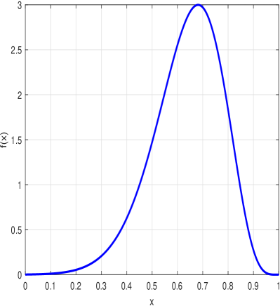
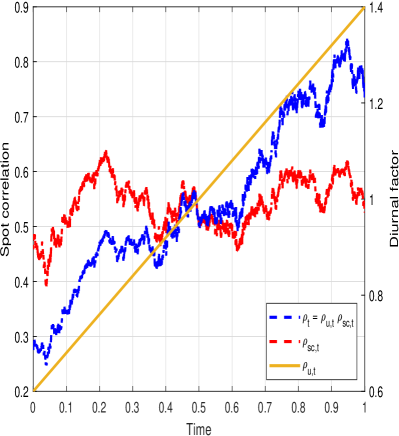
Note. In Panel A, we plot the stationary distribution of $\rho_{sc,t}$ implied by the stochastic correlation model in (71). The parameter vector is $(\kappa,\rho,\sigma)=(1.5,0.6,0.3)$. In Panel B, we show a sample path of this process with $t\in[0,1]$ and $\mathrm{d}t=1/\text{23,400}$. We further plot the diurnal correlation function $\rho_{u,t}$ from (70) with $(a,b)=(0.6,0.8)$, which together form the spot correlation $\rho_{t}=\rho_{u,t}\rho_{sc,t}$.

The above SDE can be constructed via a Fisher transformation of $\rho_{sc,t}$ (e.g., Teng, Ehrhardt, and Günther, 2016): $\displaystyle P_{sc,t}=\operatorname{arctanh}(\rho_{sc,t})=\frac{1}{2}\ln\left(\frac{1+\rho_{sc,t}}{1-\rho_{sc,t}}\right)$. Suppose $P_{sc,t}$ is a modified Gaussian Ornstein-Uhlenbeck process $\mathrm{d}P_{sc,t}=-\tilde{\kappa}\left(\tanh\left(P_{sc,t}\right)-\tilde{\rho}\right)\mathrm{d}t+\tilde{\sigma}\mathrm{d}\tilde{B}_{t}$ with $\tilde{\kappa},\tilde{\sigma}>0$ and $\tilde{\rho}\in(-1,1)$. An application of Itô’s Lemma to the inverse $\displaystyle\rho_{sc,t}=\tanh(P_{sc,t})=\frac{\exp(2P_{sc,t})-1}{\exp(2P_{sc,t})+1}$ then delivers (71) with $\sigma^{2}=\tilde{\sigma}^{2}$, $\kappa=\tilde{\kappa}+\tilde{\sigma}^{2}$ and $\displaystyle\rho=\frac{\tilde{\kappa}}{\tilde{\kappa}+\tilde{\sigma}^{2}}\tilde{\rho}$. If the parameters satisfy the “Feller”-type condition $\displaystyle\kappa>\frac{\sigma^{2}}{1\pm\rho}$, $\rho_{sc,t}$ is stationary with state space $(-1,1)$, i.e. the probability mass at the boundary goes sufficiently fast to zero as $\rho_{sc,t}\rightarrow\pm 1$, such that the barriers are not attainable (nor attractive). This is suitable for a dynamic correlation model.

We set $(\kappa,\rho,\sigma)=(1.5,0.6,0.3)$, so that the above condition is fulfilled. This means that the average value of $\rho_{sc,t}$ is 0.6, implying a modest positive association between $X$ and $Y$ in line with the descriptive statistics of the unconditional correlation presented in Table 3 in the empirical investigation. The initial condition $\rho_{sc,0}$ is drawn at random from the stationary distribution of $\rho_{sc,t}$, which is illustrated in Panel A of Figure 1. A realization of the full-blown continuous-time dynamics of $\rho_{sc,t}$ is shown in Panel B of Figure 1.

We add a pure-jump component to the continuous sample path log-price, which is simulated as a compound Poisson process:

$$\mathrm{d}J_{t}^{\bullet}=q_{t}^{\bullet}\mathrm{d}N_{t}^{\bullet},$$

where $q_{t}^{\bullet}$ is the jump size at time $t$ and $N_{t}^{\bullet}$ is a Poisson process with intensity $\lambda_{J}$. We draw $q_{t}^{\bullet}\sim N(0,\sigma_{J}^{2})$ with $\displaystyle\sigma_{J}=\sqrt{\frac{1}{\lambda_{J}}\frac{p_{J}}{1-p_{J}}V_{0}}$, so the quadratic jump variation is proportional to the average diffusive variance. $p_{J}$ controls how much of the second-order variation in the log-price process that is due to the jump component. We assume $\lambda_{J}=0.2$ and $p_{J}=0.1$, such that a jump is observed in every fifth replication, while accounting for 10% of the quadratic variation, on average. This conforms with empirical evidence on jump testing (e.g., Aït-Sahalia, Jacod, and Li, 2012; Aït-Sahalia and Xiu, 2016; Bajgrowicz, Scaillet, and Treccani, 2016).

We discretize the system with an Euler scheme and a baseline step of $\mathrm{d}t=1/23{,}400$. This represents the “continuous-time” foundation from which we extract a coarser sample of size $n=$ 26, 39, 78, 390, 780, 1,560, and 4,680, equidistant log-price increments over an interval of length $T=$ 5, 22, and 66. The former can be interpreted as discretely sampling a process every 900, 600, 300, 60, 30, 15, and 5 seconds, while the latter corresponds to observing such high-frequency data over a week, month, and quarter.

A total of 10,000 replica are made. As described in Section 3, in each simulation we divide the available high-frequency data $(\Delta_{(t-1)n+i}^{n}X)_{i=1,\dots,n\text{ and }t=1,\dots,T}$ and $(\Delta_{(t-1)n+i}^{n}Y)_{i=1,\dots,n\text{ and }t=1,\dots,T}$ into non-overlapping subsets of size $k_{n}=$ 13, 13, 26, 130, 195, 390, and 963, corresponding to $n/k_{n}=$ 2, 3, 3, 3, 4, 4, and 5, so the number of blocks is rising slowly with $n$, as required by the rate condition from Theorem 4.4. Indeed, because the testing procedure explores the properties of the covariance process, a casual robustness check suggests that is preferable with a smaller number of blocks consisting of a larger number of increments, than vice versa, as it is important to get a good approximation of its intraday dynamic.

We calculate the jump-robust bipower variation and relieve log-returns from the jump component by blockwise truncation of increments that are numerically above $v_{n}=q\sqrt{\text{BV}}n^{0.5-\varpi}$ with $q=5$ and $\varpi=0.49$. Hence, our procedure labels a log-return as a jump if it exceeds about five diffusive standard deviations.

We inspect both the nonpivotal-based test statistic derived from Theorem 4.1 and the pivotal-based test statistic derived from Theorem 4.4. Note that Assumption (C6) does not hold in our setting, so the latter should be viewed as a robustness check. In the below, we first summarize our findings for the pivotal-based test statistic and then comment on the main differences with the other one. In either case, we implement the HAC estimator with $H_{T}=[T^{1/3}]$ and a Parzen kernel. The results are robust to the concrete choice of lag length, so long as it is not exceedingly large. To evaluate the nonpivotal test statistic, we draw $9{,}999$ realizations of $\widehat{\mathcal{Z}}$ and extract an appropriate quantile from the induced empirical distribution function.

Table 1: Rejection rate of the nonpivotal-based test statistic derived from Theorem 4.1.

Panel A: $T=5$
			nominal level of 10%						nominal level of 5%						nominal level of 1%
$n$	$k_{n}$	$a=$	1.000	0.950	0.900	0.850	0.800	$a=$	1.000	0.950	0.900	0.850	0.800	$a=$	1.000	0.950	0.900	0.850	0.800
26	13		0.232	0.256	0.318	0.387	0.488		0.164	0.185	0.238	0.294	0.387		0.087	0.098	0.129	0.168	0.236
39	13		0.231	0.248	0.315	0.411	0.521		0.148	0.161	0.220	0.300	0.384		0.060	0.067	0.102	0.141	0.205
78	26		0.231	0.274	0.396	0.576	0.742		0.150	0.183	0.287	0.451	0.628		0.065	0.084	0.144	0.251	0.400
390	130		0.230	0.453	0.824	0.981	0.999		0.153	0.346	0.724	0.957	0.997		0.068	0.183	0.529	0.858	0.980
780	195		0.224	0.573	0.960	1.000	1.000		0.136	0.437	0.910	0.998	1.000		0.044	0.224	0.739	0.981	1.000
1,560	390		0.215	0.786	0.999	1.000	1.000		0.128	0.665	0.997	1.000	1.000		0.046	0.419	0.967	1.000	1.000
4,680	936		0.208	0.990	1.000	1.000	1.000		0.120	0.970	1.000	1.000	1.000		0.032	0.858	1.000	1.000	1.000
Panel B: $T=21$
			nominal level of 10%						nominal level of 5%						nominal level of 1%
$n$	$k_{n}$	$a=$	1.000	0.950	0.900	0.850	0.800	$a=$	1.000	0.950	0.900	0.850	0.800	$a=$	1.000	0.950	0.900	0.850	0.800
26	13		0.153	0.212	0.378	0.575	0.745		0.085	0.136	0.270	0.464	0.652		0.030	0.054	0.126	0.270	0.458
39	13		0.150	0.221	0.421	0.668	0.839		0.077	0.125	0.299	0.541	0.756		0.020	0.039	0.127	0.302	0.542
78	26		0.142	0.310	0.691	0.928	0.979		0.073	0.209	0.566	0.873	0.965		0.021	0.077	0.333	0.699	0.917
390	130		0.137	0.801	0.999	1.000	0.999		0.076	0.699	0.997	0.999	0.999		0.021	0.464	0.986	0.999	0.998
780	195		0.133	0.960	1.000	1.000	1.000		0.070	0.917	1.000	1.000	1.000		0.015	0.746	1.000	1.000	0.999
1,560	390		0.143	0.999	1.000	1.000	1.000		0.076	0.998	1.000	1.000	1.000		0.017	0.985	1.000	1.000	1.000
4,680	936		0.132	1.000	1.000	1.000	1.000		0.064	1.000	1.000	1.000	1.000		0.011	1.000	1.000	1.000	1.000
Panel C: $T=66$
			nominal level of 10%						nominal level of 5%						nominal level of 1%
$n$	$k_{n}$	$a=$	1.000	0.950	0.900	0.850	0.800	$a=$	1.000	0.950	0.900	0.850	0.800	$a=$	1.000	0.950	0.900	0.850	0.800
26	13		0.117	0.257	0.543	0.720	0.806		0.054	0.159	0.431	0.638	0.751		0.012	0.057	0.243	0.491	0.661
39	13		0.110	0.290	0.653	0.832	0.889		0.048	0.181	0.535	0.772	0.852		0.010	0.063	0.329	0.649	0.788
78	26		0.105	0.543	0.924	0.952	0.968		0.051	0.419	0.895	0.940	0.956		0.012	0.206	0.801	0.922	0.944
390	130		0.115	0.995	0.997	0.998	0.999		0.059	0.989	0.996	0.998	0.997		0.013	0.959	0.996	0.996	0.997
780	195		0.111	1.000	0.999	1.000	1.000		0.054	0.999	0.999	0.999	1.000		0.011	0.999	0.999	0.999	0.999
1,560	390		0.112	1.000	1.000	1.000	1.000		0.054	1.000	1.000	1.000	1.000		0.010	1.000	1.000	1.000	1.000
4,680	936		0.106	1.000	1.000	1.000	1.000		0.052	1.000	1.000	1.000	1.000		0.009	1.000	1.000	1.000	1.000

Note. We simulate a bivariate jump-diffusion model with diurnal variation in the correlation coefficient, such that $\rho_{t}=\rho_{sc,t}\rho_{u,t}$, where $\rho_{sc,t}$ is a stochastic process and $\rho_{u,t}=a+bt$ with $b=2(1-a)$ captures the deterministic component. The hypothesis $\mathcal{H}_{0}:\int_{0}^{1}(\rho_{u,t}-1)^{2}\mathrm{d}t=0$ is tested against $\mathcal{H}_{a}:\int_{0}^{1}(\rho_{u,t}-1)^{2}\mathrm{d}t\neq 0$. In the model, the null is equivalent to $a=1$, whereas the alternative corresponds to $a\neq 1$. The table reports rejection rates of the test statistic derived from Theorem 4.1 at various levels of significance $\alpha=(0.10,0.05,0.01)$. $n$ is the number of intradaily observations over a sample period of $T$ days, while $k_{n}$ is the number of log-price increments used to compute the block-wise realized covariance estimator.

Table 2: Rejection rate of the pivotal-based test statistic from Theorem 4.4.

Panel A: $T=5$
			nominal level of 10%						nominal level of 5%						nominal level of 1%
$n$	$k_{n}$	$a=$	1.000	0.950	0.900	0.850	0.800	$a=$	1.000	0.950	0.900	0.850	0.800	$a=$	1.000	0.950	0.900	0.850	0.800
26	13		0.108	0.129	0.169	0.218	0.301		0.090	0.107	0.142	0.184	0.254		0.066	0.077	0.102	0.135	0.194
39	13		0.149	0.161	0.215	0.292	0.388		0.115	0.127	0.178	0.240	0.328		0.079	0.085	0.122	0.170	0.244
78	26		0.156	0.188	0.299	0.471	0.651		0.124	0.150	0.253	0.409	0.587		0.083	0.104	0.181	0.315	0.482
390	130		0.159	0.362	0.773	0.971	0.999		0.128	0.315	0.722	0.961	0.998		0.087	0.241	0.635	0.931	0.994
780	195		0.191	0.538	0.956	1.000	1.000		0.150	0.479	0.937	0.999	1.000		0.096	0.384	0.895	0.998	1.000
1,560	390		0.182	0.765	0.999	1.000	1.000		0.144	0.719	0.999	1.000	1.000		0.094	0.625	0.996	1.000	1.000
4,680	936		0.215	0.993	1.000	1.000	1.000		0.170	0.989	1.000	1.000	1.000		0.113	0.973	1.000	1.000	1.000
Panel B: $T=21$
			nominal level of 10%						nominal level of 5%						nominal level of 1%
$n$	$k_{n}$	$a=$	1.000	0.950	0.900	0.850	0.800	$a=$	1.000	0.950	0.900	0.850	0.800	$a=$	1.000	0.950	0.900	0.850	0.800
26	13		0.095	0.130	0.240	0.430	0.634		0.077	0.105	0.197	0.372	0.581		0.057	0.074	0.139	0.285	0.483
39	13		0.108	0.162	0.333	0.581	0.797		0.082	0.125	0.277	0.512	0.747		0.055	0.079	0.193	0.399	0.654
78	26		0.090	0.228	0.601	0.899	0.980		0.065	0.183	0.533	0.865	0.974		0.039	0.116	0.425	0.792	0.957
390	130		0.080	0.722	0.998	0.999	1.000		0.057	0.667	0.998	0.999	0.999		0.030	0.564	0.995	0.999	0.999
780	195		0.093	0.945	1.000	1.000	1.000		0.066	0.919	1.000	1.000	1.000		0.035	0.864	1.000	1.000	1.000
1,560	390		0.102	0.999	1.000	1.000	1.000		0.073	0.999	1.000	1.000	1.000		0.038	0.996	1.000	1.000	1.000
4,680	936		0.108	1.000	1.000	1.000	1.000		0.076	1.000	1.000	1.000	1.000		0.038	1.000	1.000	1.000	1.000
Panel C: $T=66$
			nominal level of 10%						nominal level of 5%						nominal level of 1%
$n$	$k_{n}$	$a=$	1.000	0.950	0.900	0.850	0.800	$a=$	1.000	0.950	0.900	0.850	0.800	$a=$	1.000	0.950	0.900	0.850	0.800
26	13		0.110	0.200	0.454	0.696	0.815		0.095	0.168	0.397	0.653	0.788		0.075	0.127	0.309	0.572	0.742
39	13		0.120	0.257	0.622	0.860	0.926		0.101	0.209	0.566	0.834	0.913		0.078	0.146	0.458	0.777	0.887
78	26		0.081	0.456	0.930	0.973	0.984		0.060	0.389	0.911	0.968	0.980		0.040	0.280	0.870	0.960	0.975
390	130		0.063	0.991	0.997	0.999	0.999		0.041	0.987	0.997	0.998	0.998		0.020	0.975	0.996	0.998	0.998
780	195		0.072	1.000	0.999	1.000	1.000		0.046	0.999	0.999	1.000	1.000		0.021	0.999	0.999	0.999	1.000
1,560	390		0.071	1.000	1.000	1.000	1.000		0.046	1.000	1.000	1.000	1.000		0.021	1.000	1.000	1.000	1.000
4,680	936		0.077	1.000	1.000	1.000	1.000		0.050	1.000	1.000	1.000	1.000		0.023	1.000	1.000	1.000	1.000

Note. We simulate a bivariate jump-diffusion model with diurnal variation in the correlation coefficient, such that $\rho_{t}=\rho_{sc,t}\rho_{u,t}$, where $\rho_{sc,t}$ is a stochastic process and $\rho_{u,t}=a+bt$ with $b=2(1-a)$ captures the deterministic component. The hypothesis $\mathcal{H}_{0}:\int_{0}^{1}(\rho_{u,t}-1)^{2}\mathrm{d}t=0$ is tested against $\mathcal{H}_{a}:\int_{0}^{1}(\rho_{u,t}-1)^{2}\mathrm{d}t\neq 0$. In the model, the null is equivalent to $a=1$, whereas the alternative corresponds to $a\neq 1$. The table reports rejection rates of the test statistic from Theorem 4.4 at various levels of significance $\alpha=(0.10,0.05,0.01)$. $n$ is the number of intradaily observations over a sample period of $T$ days, while $k_{n}$ is the number of log-price increments used to compute the block-wise realized covariance estimator.

The outcome of the exercise is presented in Tables 1 – 2. They show rejection rates of the testing procedure for the intraday sample sizes (in rows) and diurnal correlation slopes (in columns). The different values of $T$ are reported in Panel A – C.

The column headings with $a=1.00$ refer to the null hypothesis and we look at those to begin with. We observe that for $T=5$ the test is somewhat oversized, as the rejection rates are higher than the nominal level. With such a small $T$, the time-averaged block-wise realized covariance is inevitably going to be a very crude measure of the associated time-of-day spot covariance, which introduces some distortion. At $T=22$, the rejection rates have already settled around the anticipated value at the 10% nominal level, but we still see a slight overrejection at lower significance levels. The latter arises from discrepancies between the sampling distribution of the test statistic for a finite number of blocks (in the ideal situation, this is a standardized chi-squared distribution) and that predicted by the asymptotic theory (a standard normal). The former is heavy-tailed and retains a sustained positive skew for a low number of degrees of freedom (corresponding to a small number of blocks, $n/k_{n}$), and for this reason the right-hand tail remains somewhat elevated compared to that of a Gaussian density. Of course, it can potentially also be attributed to our choice of tuning parameters in the implementation, which impacts the results in finite samples. By and large, however, the numbers align with the asymptotic distribution theory under the null. We therefore leave the pursuit of more optimal tuning parameters to a future endeavour.

Moving to the right toward columns with $a\neq 1$, which defines our alternative, we observe a monotonic rise in the rejection rates as $a$ gets smaller, which steepens the slope of the intraday correlation curve, and as the sample size increases (either $n$ or $T$). This is in line with the prescribed asymptotic theory from Section 4. Note that for commonly employed intraday sample sizes (e.g. $n=78$ or $n=390$) and a month worth of high-frequency data (i.e. $T=22$), the power is rather good. This is compelling, since our naive configuration with a straight line understates the evolution of the nonlinear curve observed in practice.

The nonpivotal-based statistic is a bit more oversized for small $T$, but it appears less sensitive to the concrete value of $n$ and $k_{n}$. The rejection rates again settle around the nominal level as the time span increases under the null hypothesis, while under the alternative they are slightly higher compared to the pivotal statistic. However, the latter finding is mainly caused by the size distortion. Overall, the different test statistics largely concur in their assessment.

6 Empirical application

We conduct an assessment about the presence of diurnal variation in the empirical correlation process by studying a vast dataset covering an extended time frame and a broad selection of companies from the large-cap segment of the US stock market.

6.1 Data description

At our disposal are high-frequency data from the members of the Dow Jones Industrial Average index, as of the August 31, 2020 recomposition. In addition, we include the SPDR (formerly known as Standard & Poor’s Depository Receipts) S&P 500 trust, listed under the ticker symbol SPY. The latter is an exchange-traded fund that aims to replicate the total return of the S&P 500 index (before expenses). Its price development is therefore representative of market-wide changes in the valuation of US equities.

We downloaded a time series of transaction and quotation data for each security from the NYSE Trade and Quote (TAQ) database for the sample period January 4, 2010 to April 28, 2023. Prior to our investigation, we preprocessed the raw high-frequency data with a standard filtering algorithm to remove outliers (see, e.g., Barndorff-Nielsen, Hansen, Lunde, and Shephard, 2009; Christensen, Oomen, and Podolskij, 2014).

The US stock market is open for trading from 9:30am to 4:00pm on normal business days. However, on a regular basis most venues halt trading at an earlier time in observance of upcoming holidays. This is, for example, done before Independence Day, assuming July 3rd is a good day. In such instances, the trading session is shortened and the exchanges close at 1:00pm. As the diurnal correlation pattern on those days can be expected to deviate substantially from that on a regular business day with a usual trading schedule, we remove them from the sample. Furthermore, we purge the Flash Crash of May 6, 2010 due to its highly irregular volatility that exerts a disproportional effect on our estimation procedure. As a result, the empirical investigation is based on the $T=3{,}325$ days remaining in our sample.

In Table 3, we present a list of ticker symbols and descriptive statistics of the associated high-frequency data.

Table 3: Descriptive statistics of TAQ high-frequency data.

						versus SPY (point estimate)						versus rest (interquartile range)
Ticker		$N$	$\bar{\sigma}$	H		$\bar{\rho}$	$\hat{a}$	$\hat{b}$	$\hat{P}(\mathcal{T}>q_{1-\alpha/\#T})$			$\bar{\rho}$	$\hat{a}$	$\hat{b}$	$\hat{P}(\mathcal{T}>q_{1-\alpha/\#T})$
									$\mathcal{N}$	$\mathcal{P}$					$\mathcal{N}$	$\mathcal{P}$
AAPL		279,133	0.214	0.026		0.701	0.876	0.248	0.500	0.500		[0.354; 0.457]	[0.529; 0.687]	[0.626; 0.942]	[0.400; 0.475]	[0.575; 0.669]
AMGN		33,223	0.214	0.044		0.534	0.726	0.548	0.588	0.681		[0.331; 0.380]	[0.524; 0.590]	[0.820; 0.952]	[0.356; 0.487]	[0.581; 0.688]
AXP		38,304	0.213	0.033		0.674	0.838	0.325	0.562	0.481		[0.383; 0.486]	[0.552; 0.729]	[0.542; 0.896]	[0.431; 0.506]	[0.562; 0.675]
BA		64,796	0.268	0.030		0.594	0.837	0.325	0.550	0.512		[0.334; 0.423]	[0.507; 0.736]	[0.528; 0.986]	[0.381; 0.450]	[0.562; 0.650]
CAT		41,780	0.233	0.020		0.668	0.820	0.359	0.675	0.644		[0.379; 0.488]	[0.524; 0.729]	[0.542; 0.952]	[0.469; 0.531]	[0.631; 0.756]
CRM		46,594	0.281	0.025		0.603	0.829	0.342	0.581	0.544		[0.310; 0.414]	[0.451; 0.683]	[0.635; 1.098]	[0.356; 0.431]	[0.556; 0.662]
CSCO		108,339	0.201	0.057		0.666	0.862	0.275	0.269	0.269		[0.392; 0.458]	[0.609; 0.715]	[0.571; 0.782]	[0.344; 0.412]	[0.438; 0.537]
CVX		62,546	0.213	0.023		0.611	0.793	0.414	0.700	0.656		[0.351; 0.442]	[0.502; 0.689]	[0.622; 0.997]	[0.438; 0.531]	[0.625; 0.713]
DIS		72,947	0.202	0.031		0.662	0.838	0.323	0.600	0.550		[0.374; 0.458]	[0.542; 0.701]	[0.599; 0.916]	[0.419; 0.512]	[0.556; 0.656]
DOW		36,603	0.234	0.037		0.619	0.814	0.371	0.525	0.469		[0.361; 0.468]	[0.531; 0.745]	[0.510; 0.938]	[0.369; 0.444]	[0.519; 0.669]
GS		36,885	0.231	0.031		0.648	0.835	0.330	0.569	0.544		[0.359; 0.466]	[0.532; 0.713]	[0.574; 0.937]	[0.412; 0.519]	[0.562; 0.725]
HD		50,243	0.197	0.030		0.666	0.806	0.388	0.694	0.688		[0.407; 0.463]	[0.572; 0.661]	[0.679; 0.857]	[0.475; 0.581]	[0.637; 0.738]
HON		29,750	0.191	0.034		0.704	0.849	0.303	0.675	0.606		[0.415; 0.498]	[0.618; 0.740]	[0.519; 0.764]	[0.506; 0.581]	[0.613; 0.719]
IBM		39,641	0.169	0.029		0.672	0.778	0.443	0.738	0.700		[0.420; 0.486]	[0.579; 0.667]	[0.665; 0.841]	[0.512; 0.575]	[0.675; 0.756]
INTC		135,872	0.226	0.051		0.656	0.853	0.293	0.331	0.275		[0.361; 0.444]	[0.549; 0.707]	[0.585; 0.902]	[0.338; 0.400]	[0.431; 0.575]
JNJ		58,556	0.149	0.034		0.580	0.687	0.627	0.787	0.819		[0.365; 0.438]	[0.465; 0.597]	[0.805; 1.070]	[0.406; 0.544]	[0.619; 0.750]
JPM		112,419	0.217	0.022		0.689	0.842	0.316	0.619	0.556		[0.385; 0.488]	[0.553; 0.732]	[0.537; 0.894]	[0.438; 0.537]	[0.569; 0.744]
KO		66,613	0.149	0.051		0.571	0.694	0.612	0.644	0.694		[0.364; 0.421]	[0.503; 0.618]	[0.764; 0.995]	[0.375; 0.481]	[0.562; 0.669]
MCD		37,803	0.157	0.035		0.574	0.718	0.563	0.750	0.769		[0.367; 0.412]	[0.534; 0.586]	[0.828; 0.932]	[0.425; 0.506]	[0.631; 0.725]
MMM		28,154	0.177	0.038		0.668	0.801	0.398	0.669	0.706		[0.416; 0.482]	[0.589; 0.689]	[0.623; 0.823]	[0.494; 0.581]	[0.637; 0.750]
MRK		64,628	0.177	0.036		0.552	0.702	0.595	0.637	0.619		[0.351; 0.406]	[0.502; 0.601]	[0.798; 0.997]	[0.362; 0.456]	[0.537; 0.681]
MSFT		199,454	0.205	0.038		0.721	0.862	0.275	0.550	0.487		[0.388; 0.475]	[0.517; 0.668]	[0.664; 0.966]	[0.438; 0.506]	[0.544; 0.637]
NKE		44,202	0.204	0.026		0.639	0.797	0.406	0.662	0.619		[0.373; 0.446]	[0.525; 0.663]	[0.675; 0.949]	[0.444; 0.531]	[0.619; 0.713]
PG		56,081	0.153	0.044		0.543	0.636	0.728	0.756	0.756		[0.343; 0.414]	[0.422; 0.566]	[0.869; 1.156]	[0.412; 0.531]	[0.594; 0.744]
TRV		17,920	0.182	0.061		0.577	0.729	0.543	0.738	0.725		[0.361; 0.442]	[0.534; 0.645]	[0.710; 0.933]	[0.425; 0.537]	[0.669; 0.719]
UNH		39,641	0.218	0.042		0.552	0.724	0.551	0.694	0.738		[0.350; 0.383]	[0.530; 0.574]	[0.852; 0.941]	[0.394; 0.475]	[0.625; 0.738]
V		56,107	0.201	0.041		0.637	0.814	0.372	0.631	0.656		[0.365; 0.439]	[0.540; 0.673]	[0.654; 0.920]	[0.419; 0.494]	[0.625; 0.700]
VZ		78,106	0.161	0.037		0.512	0.670	0.660	0.644	0.650		[0.330; 0.383]	[0.501; 0.588]	[0.824; 0.998]	[0.344; 0.438]	[0.525; 0.637]
WBA		41,062	0.221	0.043		0.532	0.742	0.515	0.544	0.594		[0.343; 0.383]	[0.585; 0.656]	[0.689; 0.830]	[0.344; 0.400]	[0.550; 0.606]
WMT		60,565	0.156	0.034		0.538	0.664	0.673	0.756	0.781		[0.350; 0.398]	[0.453; 0.557]	[0.887; 1.094]	[0.388; 0.487]	[0.594; 0.706]
SPY		414,927	0.130	0.010		–	–	–	–	–		[0.571; 0.668]	[0.724; 0.838]	[0.325; 0.551]	[0.562; 0.694]	[0.544; 0.700]

Note. Ticker is the stock symbol. $N$ is the number of transaction data before previous-tick imputation to a 60-second sampling frequency. $\bar{\sigma}$ is the truncated realized variance of Mancini (2009) converted to an annualized standard deviation. H is the rejection rate of the Hausman test for microstructure noise described in Aït-Sahalia and Xiu (2019). $\bar{\rho}$ is the sample correlation coefficient. $(\hat{a},\hat{b})$ are OLS estimates of the parametric diurnal correlation function from (70). We implement the test of no diurnal correlation $\mathcal{H}_{0}:\int_{0}^{1}(\rho_{u,t}-1)^{2}\mathrm{d}t=0$ each month. The sample period is January 4, 2010 to April 28, 2023. $\hat{P}(\mathcal{T}>q_{1-\alpha/\#T})$ is the associated fraction of the nonpivotal-based test statistic derived from Theorem 4.1 ($\mathcal{T}=\mathcal{N}$) and the pivotal-based test statistic derived from Theorem 4.4 ($\mathcal{T}=\mathcal{P}$) that exceed the $(1-\alpha/\#T)$-quantile of the appropriate limiting distribution described in the main text, where $\alpha=0.01$ is the overall significance level and $\#T$ is the total number of hypothesis tested. We employ a Bonferroni correction to control the family-wise error rate.

We construct a 60-second equidistant transaction price series from the cleaned high-frequency data using the previous-tick rule of Wasserfallen and Zimmermann (1985), so we collect $n=390$ high-frequency returns per day for each asset. Although the asymptotic theory requires $n\rightarrow\infty$ and the amount of tick-by-tick data is an order of magnitude larger—as evident from column “$N$” in Table 3—a 60-second window is the smallest time gap at which the data can be perceived noise-free, as gauged by the Aït-Sahalia and Xiu (2019) Hausman test for microstructure noise. We compute their test statistic at the daily horizon and report the rejection rate in the “H” column in Table 3. This should be compared to a 1% level of significance. Apart from a few stocks, the rejection rate is typically close to the nominal level, showing that noise is not a major concern. Meanwhile, lowering the sampling frequency further raises the rejection rate materially (unreported, but available at request) and is not recommendable, unless a noise-robust approach is adopted.

Figure 2: A representative diurnal covariance and correlation function.

Panel A: Diurnal covariance.	Panel B: Diurnal correlation.

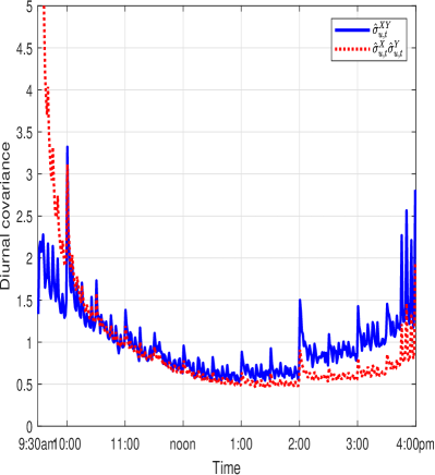
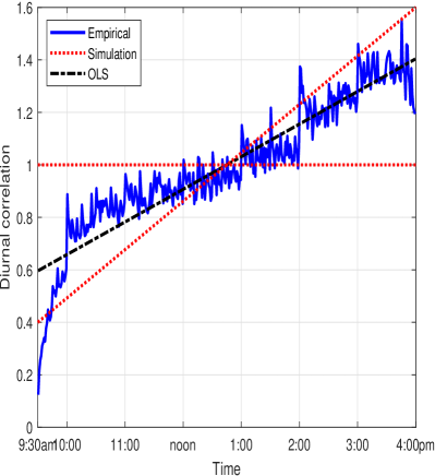
Note. In Panel A, we report a jump-robust estimator of the diurnal covariance function, $\hat{\sigma}_{u,t}^{XY}$, and compare it to $\hat{\sigma}_{u,t}^{X}\hat{\sigma}_{u,t}^{Y}$, where the latter is the imputed diurnal covariation in absence of deterministic variation in the intraday correlation coefficient, $\rho_{u,t}$. The estimator $\hat{\rho}_{u,t}$ is reported in Panel B. “OLS” is the least squares regression $\rho_{u,t}=a+bt$ [with the restriction $b=2(1-a)$] fitted to $\hat{\rho}_{u,t}$. “Simulation” shows the range of $a$ and $b$ values that are inspected in the Monte Carlo in Section 5.

6.2 The diurnal pattern in correlation

In Panel A of Figure 2, we plot a representative example of the diurnal covariance pattern inherent in our data. We follow Christensen, Hounyo, and Podolskij (2018) and compute it as the 0.5% trimmed mean realized covariance estimate (after jump-truncation) at a fixed 60-second time-of-day slot, where the average is taken across the $T=3{,}325$ days in the sample and $\displaystyle\frac{d(d-1)}{2}=465$ pairwise combinations of the number of included equities, $d$. We contrast this to the geometric mean of the idiosyncratic diurnal variance, $\hat{\sigma}_{u,t}^{X}\hat{\sigma}_{u,t}^{Y}$ (everything is normalized as in Assumption (C2) to be comparable). Since $\sigma_{u,t}^{XY}=\sigma_{u,t}^{X}\sigma_{u,t}^{Y}\rho_{u,t}$, the latter can be interpreted as the imputed diurnal covariance pattern present with no seasonality in the intraday correlation (i.e., $\rho_{u,t}=1$). In agreement with prior literature (e.g., Andersen and Bollerslev, 1997; Bibinger, Hautsch, Malec, and Reiss, 2019; Christensen, Hounyo, and Podolskij, 2018), $\hat{\sigma}_{u,t}^{X}\hat{\sigma}_{u,t}^{Y}$ resembles a “tilted J.” In contrast, we observe the actual diurnal covariance, $\hat{\sigma}_{u,t}^{XY}$, is almost symmetric and much closer to U-shaped. This is anecdotal evidence that $\rho_{u,t}$ is not always equal to one.

Next, we map each 60-second pairwise realized covariance matrix into a correlation estimate and repeat the above averaging procedure. The ensuing time-of-day correlation measure—portrayed in Panel B of Figure 2—should be randomly distributed around one under the null of no diurnal variation. Instead, we observe a pronounced upward-sloping and almost piecewise linear curve. There is notably lower (on average less positive) correlation in the morning than in the afternoon, which is in accord with Allez and Bouchaud (2011) and Hansen and Luo (2023). These findings are further corroborated by estimating the equation $\rho_{u,t}=a+bt$ in (70) from the empirical high-frequency data. The OLS parameter estimates, subject to the maintained restriction $b=2(1-a)$, are $\hat{a}=0.5969$ and $\hat{b}=0.8062$ with the fitted regression line inserted into the figure as a reference point. In practice, of course, $\rho_{u,t}$ evolves in a much more nonlinear and discontinuous fashion. We notice a positive jump at 10:00am, arguably caused by the publication of macroeconomic information. There is a another upsurge around 2:00pm, corresponding to the release of minutes from Federal Open Market Committee (FOMC) meetings.

The right-hand side of Table 3 has further descriptive statistics on diurnal correlation. It also reports the outcome of our testing procedure. We proceed as in Section 5 in terms of tuning parameters, i.e. for $n=390$ we take $k_{n}=130$. We calculate the nonpivotal- and pivotal-based test statistic each month (of which there are 160 in total) with a Parzen kernel and lag length $H_{T_{m}}=[T_{m}^{1/3}]$, where $T_{m}$ is the number of days in month $m$ (with $T_{m}=21$ on average). The analysis is then divided in two: We correlate individual members of the DJIA index against the SPY (“versus SPY”) and summarize with the interquartile range the results of pairing each stock—including the SPY—against all the thirty remaining ones (“versus rest”).

Gauging at the “versus SPY” part, several interesting findings emerge. First, every asset is positively related with the stock market portfolio exhibiting a typical level of correlation $\bar{\rho}=0.556$. Second, on an individual stock basis the estimated $a$ and $b$ parameters are broadly in line with the aggregate figures reported above and remarkably consistent over the cross-section of equities. In the end, it translates into an average rejection rate of around two thirds with either version of our test statistic. Apart from a few instances, the latter are remarkably close for the vast majority of the assets.

Switching to the “versus rest” part, on the one hand single names display a weaker association with each other than with the market, which is as expected. On the other hand, there is a tendency for the intraday correlation to exhibit a stronger linear association with $a$ being lower and $b$ being higher vis-à-vis the market. Interestingly, there is a somewhat larger discrepancy between the nonpivotal- and pivotal-based test statistic for individual assets tested against each other, where the latter is in line with the findings for the market index, whereas the former is notably lower, but it remains far above the asymptotic level.

Overall, our results suggest diurnal variation in the correlation process is a nontrivial effect, which is present most of the months in our sample.

6.3 Implications for risk management

In the closing, we highlight the importance of incorporating diurnal variation in the correlation process as exemplified via the operations of a trading desk. We suppose a dealer is long one stock from the DJIA index. The risk is offset with a dynamic short position in the market index (SPY in our context). We assume the trader employs a conventional five-minute frequency and updates the hedge at the end of each time interval—based on available information—in order to minimize the expected variance of the combined portfolio during the next five-minute window. The minimum variance hedge ratio, denoted $\phi_{i\mid i-1}^{n}$, is an adapted discrete-time stochastic process that is selected at the beginning of the $i$th interval $[(i-1)/n,i/n]$ via the following optimization problem:

$$\phi_{i\mid i-1}^{n}=\underset{\phi}{\operatorname{arg\,min}}\ \text{var}\left(\Delta_{i}^{n}X-\phi\Delta_{i}^{n}Y\mid\mathcal{F}_{\frac{i-1}{n}}\right).$$ (72)

The solution is given by:

$$\phi_{i\mid i-1}^{n}=\frac{\text{cov}\left(\Delta_{i}^{n}X,\Delta_{i}^{n}Y\mid\mathcal{F}_{\frac{i-1}{n}}\right)}{\text{var}\left(\Delta_{i}^{n}Y\mid\mathcal{F}_{\frac{i-1}{n}}\right)},$$ (73)

for $i=1,\ldots,n$, where $\Delta_{i}^{n}X$ is the subsequent five-minute log-return on the underlying asset and $\Delta_{i}^{n}Y$ is the associated SPY log-return (note that in this subsection we set $n=78$ to represent a five-minute frequency for notational convenience).

The trading policy depends on the conditional covariance matrix:

$$\Sigma_{i\mid i-1}^{n}=\text{var}\left(\begin{matrix}\Delta_{i}^{n}X\\ \Delta_{i}^{n}Y\end{matrix}\mid\mathcal{F}_{\frac{i-1}{n}}\right).$$ (74)

In practice, $\Sigma_{i\mid i-1}^{n}$ is not known in advance and has to be modeled. However, we do not pursue this approach here. Instead, we assume that an estimator of $\Sigma_{i\mid i-1}^{n}$ is accessible via the 5-minute ex-post realized covariance matrix of $X$ and $Y$ (calculated from the 60-second high-frequency data extracted above).

$\phi_{i\mid i-1}^{n}$ is then selected as:

$$\phi_{i\mid i-1}^{n}=\hat{\rho}_{[i-1,i]}\frac{\hat{\sigma}_{[i-1,i]}^{X}}{\hat{\sigma}_{[i-1,i]}^{Y}},$$ (75)

with $\hat{\sigma}_{[i-1,i]}^{X}$ and $\hat{\sigma}_{[i-1,i]}^{Y}$ being the square-root realized variance of $X$ and $Y$ on the $i$th interval, whereas $\hat{\rho}_{[i-1,i]}$ is the realized correlation.

In other words, $\phi_{i\mid i-1}^{n}$ is the ex-post minimum variance hedge ratio, conditional on knowing the subsequent realized covariance matrix over that window. It follows that $(\phi_{i\mid i-1}^{n})_{i=1}^{n}$ adapts to intraday seasonality in both the variance and correlation processes. Suppose that the stochastic correlation component is constant within a day, i.e. $\rho_{t}=\rho_{sc,\lfloor t\rfloor}\rho_{u,t}$, where $\rho_{sc,\lfloor t\rfloor}$ is determined at the start of day $t$. This assumption is common in the discrete-time multivariate stochastic volatility literature, and it is a decent approximation to the dynamic of the stochastic correlation process in view of its persistence. In this case, the high-frequency correlation estimate can be decomposed as $\hat{\rho}_{[i-1,i]}=\hat{\rho}_{u,[i-1,i]}\hat{\rho}_{sc}$, where $\hat{\rho}_{sc}=n^{-1}\sum_{i=1}^{n}\hat{\rho}_{[i-1,i]}$ is the average realized correlation over the whole day and $\hat{\rho}_{u,[i-1,i]}$ is the diurnal coefficient. This further implies that

$$\phi_{i\mid i-1}^{n}=\hat{\rho}_{u,[i-1,i]}\hat{\rho}_{sc}\frac{\hat{\sigma}_{[i-1,i]}^{X}}{\hat{\sigma}_{[i-1,i]}^{Y}}=\hat{\rho}_{u,[i-1,i]}\bar{\phi}_{i\mid i-1}^{n},$$ (76)

where ${\bar{\phi}}_{i\mid i-1}^{n}$ is the optimal ex-post hedge ratio, when the local correlation estimate is replaced by an average for the entire day, all else equal. Hence, ${\bar{\phi}}_{i\mid i-1}^{n}$ adapts to diurnal variation in the variance but not the correlation.

Figure 3: The distribution of the minimum variance hedge ratio.

Panel A: intraday evolution.	Panel B: unconditional distribution.

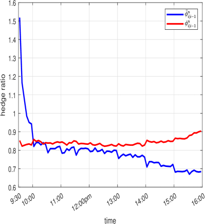
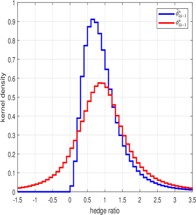
Note. In Panel A, we plot the evolution of the average intraday minimum variance hedge ratio, i.e. $\phi_{i\mid i-1}^{n}$ and $\bar{\phi}_{i\mid i-1}^{n}$. In Panel B, we show unconditional distribution of $\phi_{i\mid i-1}^{n}$ and $\bar{\phi}_{i\mid i-1}^{n}$.

We compare $\phi_{i\mid i-1}^{n}$ and $\bar{\phi}_{i\mid i-1}^{n}$ to illustrate the effect on risk management. The minimum variance hedge ratio is computed as described above across the components of the DJIA index and for each 5-minute interval in the sample. Figure 3 reports the results. In Panel A, we plot the intraday profile of $\phi_{i\mid i-1}^{n}$ and $\bar{\phi}_{i\mid i-1}^{n}$. The optimal $\phi_{i\mid i-1}^{n}$ is around 0.7 – 0.8. In contrast, there is pronounced variation in $\bar{\phi}_{i\mid i-1}^{n}$. The latter fails to acknowledge that lower correlation in the morning has a detrimental impact on the diversification effect, causing a reduced hedge ratio (and vice versa in the afternoon). Interestingly, this means there are fewer transaction costs associated with managing a portfolio based on $\phi_{i\mid i-1}^{n}$. In Panel B, we see the unconditional distribution of $\phi_{i\mid i-1}^{n}$ is more symmetric and has mass below zero, as it automatically adapts to brief lapses of low-to-negative correlation. In contrast, the histogram of $\bar{\phi}_{i\mid i-1}^{n}$ is floored at zero, because the daily correlation with the stock index tends to be positive.

The variance ratio of the full sample ex-post portfolio return:

$$\frac{\widehat{\text{var}}(\Delta_{i}^{n}X-\phi_{i\mid i-1}^{n}\Delta_{i}^{n}Y)}{\widehat{\text{var}}(\Delta_{i}^{n}X-\bar{\phi}_{i\mid i-1}^{n}\Delta_{i}^{n}Y)}=0.824,$$ (77)

suggesting it is possible to achieve a highly nontrivial reduction in risk exposure of about 17.6% in a risk management model that controls for diurnal variation in correlation.

7 Conclusion

We document pervasiveness in the intraday correlation dynamics in the US equity market. As consistent with Allez and Bouchaud (2011), Bibinger, Hautsch, Malec, and Reiss (2019), and Hansen and Luo (2023), correlations start out low in the morning and rise systematically during the trading session with notable spikes around the release of macroeconomic information. We develop a nonparametric test of the hypothesis that there is no diurnal variation in the correlation process. The test statistic has a known distribution under the null, whereas it diverges under an alternative with deterministic variation in the correlation. In a simulation study, the testing procedure aligns closely with these predictions and it attains a good rejection rate for moderate sample sizes and realistic shapes in the diurnal correlation process.

Andersen, Thyrsgaard, and Todorov (2019) test whether the intraday volatility curve is changing over time (see Andersen, Su, Todorov, and Zhang, 2023, for related work). They exploit an assumed stationarity of the stochastic volatility and compare the unconditional distribution of different time-of-the-day high-frequency returns. As in this paper, their results are derived based on a combination of infill and long-span analysis. It may be possible to adapt that setting to our framework by feeding their test statistic with devolatized high-frequency returns. We leave this idea for inspiration.

Appendix A Proofs

In this appendix, we prove the theoretical results presented in the main text. To facilitate the derivations, we denote the continuous part of $X$ and $Y$ by

$$X^{c}\equiv X_{0}+\int_{0}^{t}a^{X}\mathrm{d}s+\int_{0}^{t}\sigma_{s}^{X}\mathrm{d}W_{s}^{X}\quad\text{and}\quad Y^{c}\equiv Y_{0}+\int_{0}^{t}a^{Y}\mathrm{d}s+\int_{0}^{t}\sigma_{s}^{Y}\left(\rho_{s}\mathrm{d}W_{s}^{X}+\sqrt{1-\rho_{s}^{2}}\mathrm{d}W_{s}^{Y}\right).$$

We set $e^{XY}_{t,\tau}=\hat{c}_{t,\tau}^{XY}-\hat{c}_{t,\tau}^{X^{c}Y^{c}}$ for $t=1,\dots,T$ and $\tau\in[0,1)$, which is the block-wise difference between the realized covariance calculated on the whole process or only its continuous component. We also denote $i_{t,j}=t-1+(j-1)k_{n}\Delta_{n}$ and write $U_{t,j}=U_{i_{t,j}}$ for any stochastic process $U$.

Furthermore, we define

$$\zeta_{1}^{n}(t,\tau_{j}) =\frac{n}{k_{n}}\sum_{\ell=(j-1)k_{n}+1}^{jk_{n}}\int_{i_{t,\ell}}^{i_{t,\ell+1}}a_{s}^{X}\mathrm{d}s\cdot\int_{i_{t,\ell}}^{i_{t,\ell+1}}a_{s}^{Y}\mathrm{d}s,$$

$$\zeta_{2}^{n}(t,\tau_{j}) =\frac{n}{k_{n}}\sum_{\ell=(j-1)k_{n}+1}^{jk_{n}}\int_{i_{t,\ell}}^{i_{t,\ell+1}}a_{s}^{X}\mathrm{d}s\cdot\int_{i_{t,\ell}}^{i_{t,\ell+1}}\sigma_{s}^{Y}\left(\rho_{s}\mathrm{d}W_{s}^{X}+\sqrt{1-\rho_{s}^{2}}\mathrm{d}W_{s}^{Y}\right),$$

$$\zeta_{3}^{n}(t,\tau_{j}) =\frac{n}{k_{n}}\sum_{\ell=(j-1)k_{n}+1}^{jk_{n}}\int_{i_{t,\ell}}^{i_{t,\ell+1}}a_{s}^{Y}\mathrm{d}s\cdot\int_{i_{t,\ell}}^{i_{t,\ell+1}}\sigma_{s}^{X}\mathrm{d}W_{s}^{X},$$

$$\zeta_{4}^{n}(t,\tau_{j}) =\frac{n}{k_{n}}\sum_{\ell=(j-1)k_{n}+1}^{jk_{n}}\int_{i_{t,\ell}}^{i_{t,\ell+1}}\left(\sigma_{s}^{X}-\sigma_{t,j}^{X}\right)\mathrm{d}W_{s}^{X}\cdot\int_{i_{t,\ell}}^{i_{t,\ell+1}}\sigma_{s}^{Y}\left(\rho_{s}\mathrm{d}W_{s}^{X}+\sqrt{1-\rho_{s}^{2}}\mathrm{d}W_{s}^{Y}\right),$$

$$\zeta_{5}^{n}(t,\tau_{j}) =\frac{n}{k_{n}}\sum_{\ell=(j-1)k_{n}+1}^{jk_{n}}\int_{i_{t,\ell}}^{i_{t,\ell+1}}\sigma_{s}^{X}\mathrm{d}W^{X}_{s}\cdot\int_{i_{t,\ell}}^{i_{t,\ell+1}}\left(\sigma_{s}^{Y}-\sigma_{t,j}^{Y}\right)\left(\rho_{s}\mathrm{d}W_{s}^{X}+\sqrt{1-\rho_{s}^{2}}\mathrm{d}W_{s}^{Y}\right),$$

$$\zeta_{6}^{n}(t,\tau_{j}) =\frac{n}{k_{n}}\sum_{\ell=(j-1)k_{n}+1}^{jk_{n}}\int_{i_{t,\ell}}^{i_{t,\ell+1}}\left(\sigma_{s}^{X}-\sigma_{t,j}^{X}\right)\mathrm{d}W_{s}^{X}\cdot\int_{i_{t,\ell}}^{i_{t,\ell+1}}\left(\sigma_{s}^{Y}-\sigma_{t,j}^{Y}\right)\left(\rho_{s}\mathrm{d}W_{s}^{X}+\sqrt{1-\rho_{s}^{2}}\mathrm{d}W_{s}^{Y}\right).$$

We are going to need a couple of auxiliary lemmas.

Lemma A.1

Suppose the boundedness condition in Assumption (C4) holds. Then, for $i=1,\dots,3$:

$$\mathrm{\mathbb{E}}\left(\left|\frac{1}{T}\sum_{t=1}^{T}\zeta_{i}^{n}(t,\tau_{j})\right|^{m}\right)\leq\frac{C}{n^{m}},$$

for any $m\geq 2$ and $\tau_{j}\in[0,1]$.

Proof: The term $\frac{1}{T}\sum_{t=1}^{T}\zeta_{1}^{n}(t,\tau_{j})$ is handled with Jensen’s inequality and the $C_{r}$ inequality:

$$\mathbb{E}\left(\left|\frac{1}{T}\sum_{t=1}^{T}\zeta_{1}^{n}(t,\tau_{j})\right|^{m}\right) \leq\frac{n^{m}}{Tk_{n}}\sum_{t=1}^{T}\sum_{\ell=(j-)k_{n}+1}^{jk_{n}}\mathbb{E}\left[\left(\int_{i_{t,\ell}}^{i_{t,\ell+1}}a_{s}^{X}\mathrm{d}s\cdot\int_{i_{t,\ell}}^{i_{t,\ell+1}}a_{s}^{Y}\mathrm{d}s\right)^{m}\right]$$

$$\leq\frac{C_{m}n^{m}}{Tk_{n}}\sum_{t=1}^{T}\sum_{\ell=(j-1)k_{n}+1}^{jk_{n}}\mathbb{E}\left[\left(\int_{i_{t,\ell}}^{i_{t,\ell+1}}a_{s}^{X}\mathrm{d}s\right)^{2m}+\left(\int_{i_{t,\ell}}^{i_{t,\ell+1}}a_{s}^{Y}\mathrm{d}s\right)^{2m}\right]$$

$$\leq\frac{C_{m}}{Tk_{n}n^{m-1}}\sum_{t=1}^{T}\sum_{\ell=(j-1)k_{n}+1}^{jk_{n}}\left(\int_{i_{t,\ell}}^{i_{t,\ell+1}}\mathbb{E}\left(a_{s}^{X}\right)^{2m}\mathrm{d}s+\int_{i_{t,\ell}}^{i_{t,\ell+1}}\mathbb{E}\left(a_{s}^{Y}\right)^{2m}\mathrm{d}s\right)$$

$$\leq\frac{C}{n^{m}},$$

where the first line in the array is based on the trivial inequality $ab\leq a^{2}+b^{2}$ and the last line is due to the boundedness condition.

The treatment of the second and third term is nearly identical, so here we only verify the proof of the latter. By the Cauchy-Schwarz inequality, Jensen’s inequality, the Itô isometry, and the boundedness condition, we observe that

$$\mathbb{E}\left(\left|\frac{1}{T}\sum_{t=1}^{T}\zeta_{3}^{n}(t,\tau_{j})\right|^{m}\right) \leq\frac{n^{m}}{Tk_{n}}\sum_{t=1}^{T}\sum_{\ell=(j-1)k_{n}+1}^{jk_{n}}\mathbb{E}\left(\left|\int_{i_{t,\ell}}^{i_{t,\ell+1}}a_{s}^{Y}\mathrm{d}s\cdot\int_{i_{t,\ell}}^{i_{t,\ell+1}}\sigma_{s}^{X}\mathrm{d}W_{s}^{X}\right|^{m}\right)$$

$$\leq\frac{n^{m}}{Tk_{n}}\sum_{t=1}^{T}\sum_{\ell=(j-1)k_{n}+1}^{jk_{n}}\left[\mathbb{E}\left(\left|\int_{i_{t,\ell}}^{i_{t,\ell+1}}a_{s}^{Y}\mathrm{d}s\right|^{2m}\right)\cdot\mathbb{E}\left(\left|\int_{i_{t,\ell}}^{i_{t,\ell+1}}\sigma_{s}^{X}\mathrm{d}W_{s}^{X}\right|^{2m}\right)\right]^{1/2}$$

$$\leq\frac{C}{Tk_{n}n^{m/2-1}}\sum_{t=1}^{T}\sum_{\ell=(j-1)k_{n}+1}^{jk_{n}}\left(\int_{i_{t,\ell}}^{i_{t,\ell+1}}\mathbb{E}\left(a_{s}^{Y}\right)^{2m}\mathrm{d}s\cdot\int_{i_{t,\ell}}^{i_{t,\ell+1}}\mathbb{E}\left(\sigma_{s}^{X}\right)^{2m}\mathrm{d}s\right)^{1/2}$$

$$\leq\frac{C}{n^{m/2}}.$$

$\blacksquare$

Lemma A.2

Suppose the boundedness condition in Assumption in (C4) holds. Then,

$$\mathbb{E}\left(\left|\frac{1}{T}\sum_{t=1}^{T}\zeta_{4}^{n}(t,\tau_{j})\right|\right)\leq\frac{C}{n^{1/2}},\quad\mathbb{E}\left(\left|\frac{1}{T}\sum_{t=1}^{T}\zeta_{5}^{n}(t,\tau_{j})\right|\right)\leq\frac{C}{n^{1/2}},\quad\text{and }\mathbb{E}\left(\left|\frac{1}{T}\sum_{t=1}^{T}\zeta_{6}^{n}(t,\tau_{j})\right|\right)\leq\frac{C}{n}.$$

Proof: By the $C_{r}$ inequality, Burkholder-Davis-Gundy inequality, Assumption (V), and the boundedness condition, for $s\in[i_{t,j},i_{t,j+1}]$, we find that

$$\mathbb{E}\left(|\sigma_{s}^{X}-\sigma_{t,j}^{X}|^{2}\right) \leq C\Bigg{[}\mathbb{E}\left(\int_{i_{t,j}}^{s}\tilde{a}_{u}^{X}\mathrm{d}u\right)^{2}+\mathbb{E}\left(\int_{i_{t,j}}^{s}\tilde{\sigma}_{u}^{X}\mathrm{d}W_{u}^{X}\right)^{2}+\mathbb{E}\left(\int_{i_{t,j}}^{s}\tilde{\sigma}_{u}^{Y}\mathrm{d}W_{u}^{Y}\right)^{2}$$

$$+\mathbb{E}\left(\int_{i_{t,j}}^{s}\tilde{\nu}_{u}^{X}\mathrm{d}\tilde{W}_{u}^{X}\right)^{2}+\mathbb{E}\left(\int_{i_{t,j}}^{s}\tilde{\nu}_{u}^{Y}\mathrm{d}\tilde{W}_{u}^{Y}\right)^{2}+\mathbb{E}\left(\int_{i_{t,j}}^{s}\int_{\mathbb{R}}x\tilde{F}_{x}^{X}\mathrm{d}x\mathrm{d}u\right)^{2}\Bigg{]}\leq\frac{C}{n}.$$

After another round with the Cauchy-Schwarz inequality, Jensen’s inequality, the Itô isometry, and the boundedness condition, we arrive at the conclusion that

$$\mathbb{E}\left(\left|\frac{1}{T}\sum_{t=1}^{T}\zeta_{4}^{n}(t,\tau_{j})\right|\right) \leq\frac{Cn}{Tk_{n}}\sum_{t=1}^{T}\sum_{\ell=(j-1)k_{n}+1}^{jk_{n}}\left(\int_{i_{t,\ell}}^{i_{t,\ell+1}}\mathbb{E}\left(\sigma_{s}^{X}-\sigma_{t,j}^{X}\right)^{2}\mathrm{d}s\cdot\int_{i_{t,\ell}}^{i_{t,\ell+1}}\mathbb{E}\left(\sigma_{s}^{Y}\right)^{2}\mathrm{d}s\right)^{1/2}$$

$$\leq\frac{C}{n^{1/2}}.$$

The proofs of the other inequalities follow the same footsteps. $\blacksquare$

Proof of Theorem 3.1: It suffices to prove the convergence for the covariance term, $\hat{c}_{u,\tau}^{XY}$, for $\tau\in[0,1]$. We begin with a decomposition of the continuous part of $\hat{c}_{t,\tau_{j}}^{XY}$, i.e. $\hat{c}_{t,\tau_{j}}^{X^{c}Y^{c}}$:

$$\hat{c}_{t,\tau_{j}}^{X^{c}Y^{c}} =\frac{n}{k_{n}}\sum_{\ell=(j-1)k_{n}+1}^{jk_{n}}\Delta_{(t-1)n+\ell}^{n}X^{c}\Delta_{(t-1)n+\ell}^{n}Y^{c}$$

$$=\sum_{m=1}^{6}\zeta_{m}^{n}(t,\tau_{j})+\sigma_{t,j}^{X}\sigma_{t,j}^{Y}\rho_{t,j}\cdot\frac{n}{k_{n}}\sum_{\ell=(j-1)k_{n}+1}^{jk_{n}}(\Delta_{(t-1)n+\ell}^{n}W^{X})^{2}$$

$$+\sigma_{t,j}^{X}\sigma_{t,j}^{Y}\sqrt{1-\rho_{t,j}^{2}}\cdot\frac{n}{k_{n}}\sum_{\ell=(j-1)k_{n}+1}^{jk_{n}}\Delta_{(t-1)n+\ell}^{n}W^{X}\Delta_{(t-1)n+\ell}^{n}W^{Y}$$

$$=\sum_{m=1}^{6}\zeta_{m}^{n}(t,\tau_{j})+\sigma_{t,j}^{X}\sigma_{t,j}^{Y}\rho_{t,j}\cdot\alpha_{t,j}^{n}+\sigma_{t,j}^{X}\sigma_{t,j}^{Y}\sqrt{1-\rho_{t,j}^{2}}\cdot\beta_{t,j}^{n},$$

where

$$\alpha_{t,j}^{n}=\frac{n}{k_{n}}\sum_{\ell=(j-1)k_{n}+1}^{jk_{n}}(\Delta_{(t-1)n+\ell}^{n}W^{X})^{2},\quad\beta_{t,j}^{n}=\frac{n}{k_{n}}\sum_{\ell=(j-1)k_{n}+1}^{jk_{n}}\Delta_{(t-1)n+\ell}^{n}W^{X}\Delta_{(t-1)n+\ell}^{n}W^{Y},$$

and $\zeta_{m}^{n}(t,\tau_{j})$ is defined in the preparation step at the beginning of this appendix. Thus, according to Assumption (C1):

$$\hat{c}_{t,\tau_{j}}^{XY} =\sigma_{u,j}^{X}\sigma_{u,j}^{Y}\rho_{u,j}\cdot\sigma_{sv,t,j}^{X}\sigma_{sv,t,j}^{Y}\rho_{sv,t,j}\cdot\alpha_{t,j}^{n}+\sigma_{t,j}^{X}\sigma_{t,j}^{Y}\sqrt{1-\rho_{t,j}^{2}}\cdot\beta_{t,j}^{n}+\sum_{m=1}^{6}\zeta_{m}^{n}(t,\tau_{j})$$

$$=\sigma_{u,j}^{X}\sigma_{u,j}^{Y}\rho_{u,j}\cdot\sigma_{sv,t,j}^{X}\sigma_{sv,t,j}^{Y}\rho_{sv,t,j}$$

$$+\sigma_{u,j}^{X}\sigma_{u,j}^{Y}\rho_{u,j}\cdot\sigma_{sv,t,j}^{X}\sigma_{sv,t,j}^{Y}\rho_{sv,t,j}\cdot(\alpha_{t,j}^{n}-1)+\sigma_{t,j}^{X}\sigma_{t,j}^{Y}\sqrt{1-\rho_{t,j}^{2}}\cdot\beta_{t,j}^{n}+\sum_{m=1}^{6}\zeta_{m}^{n}(t,\tau_{j}).$$

Therefore,

$$\tilde{c}_{u,\tau_{j}}^{XY} =\frac{1}{T}\sum_{t=1}^{T}\hat{c}_{t,\tau_{j}}^{X^{c}Y^{c}}+\frac{1}{T}\sum_{i=1}^{T}e^{XY}_{t,\tau_{j}}$$

$$=\sigma_{u,j}^{X}\sigma_{u,j}^{Y}\rho_{u,j}\cdot\frac{1}{T}\sum_{t=1}^{T}\sigma_{sv,t,j}^{X}\sigma_{sv,t,j}^{Y}\rho_{sv,t,j}+\frac{1}{T}\sum_{i=1}^{T}e^{XY}_{t,\tau_{j}}+\sum_{m=1}^{6}\left(\frac{1}{T}\sum_{t=1}^{T}\zeta_{m}^{n}(t,\tau_{j})\right)$$

$$+\frac{1}{T}\sum_{t=1}^{T}\left(\sigma_{u,j}^{X}\sigma_{u,j}^{Y}\rho_{u,j}\cdot\sigma_{sv,t,j}^{X}\sigma_{sv,t,j}^{Y}\rho_{sv,t,j}\cdot(\alpha_{t,j}^{n}-1)+\sigma_{t,j}^{X}\sigma_{t,j}^{Y}\sqrt{1-\rho_{t,j}^{2}}\cdot\beta_{t,j}^{n}\right)$$

$$\equiv\sigma_{u,j}^{X}\sigma_{u,j}^{Y}\rho_{u,j}\cdot\frac{1}{T}\sum_{t=1}^{T}\sigma_{sv,t,j}^{X}\sigma_{sv,t,j}^{Y}\rho_{sv,t,j}+\mathrm{I}_{j,n,T}+\mathrm{II}_{j,n,T}+\mathrm{III}_{j,n,T}.$$

First, we observe that by the polarization identity and Lemma 12 of Andersen, Su, Todorov, and Zhang (2023), it readily holds that

$$\mathbb{E}\big{(}|\mathrm{I}_{j,n,T}|\big{)}=\mathbb{E}\left(\left|\frac{1}{T}\sum_{t=1}^{T}e^{XY}_{t,\tau_{j}}\right|\right)\leq Cn^{-2\varpi},$$

where $\varpi\in(0,1/2)$. Hence, $\mathbb{E}\big{(}|\mathrm{I}_{j,n,T}|\big{)}\rightarrow 0$. Second, the convergence $\mathbb{E}\big{(}|\mathrm{II}_{j,n,T}|\big{)}\rightarrow 0$ is a direct consequence of Lemmas 1 – 2. Third, it is straightforward to deduce that

$$\mathbb{E}\big{[}(\alpha_{t,j}^{n}-1)^{2}\big{]}\leq\frac{C}{k_{n}}\quad\mathrm{and}\quad\mathbb{E}\big{[}(\beta_{t,j}^{n})^{2}\big{]}\leq\frac{C}{k_{n}},$$

uniformly in $t$ and $j$. Thus, by the boundedness condition $\mathbb{E}\big{(}|\mathrm{III}_{j,n,T}|\big{)}\rightarrow 0$.

We write

$$\eta\equiv\mathbb{E}\left(\sigma_{sv,t,j}^{X}\sigma_{sv,t,j}^{Y}\rho_{sv,t,j}\right)=\mathbb{E}\left(c_{sv,1}^{XY}\right).$$

By applying the law of iterated expectations, Hölder’s inequality and the mixing property in Assumption (C5), for any $\omega>1(1+\ell)/\ell$,

$$\mathbb{E}\left[\left(\frac{1}{T}\sum_{t=1}^{T}\sigma_{sv,t,j}^{X}\sigma_{sv,t,j}^{Y}\rho_{sv,t,j}-\eta\right)^{2}\right]$$

$$=\frac{2}{T^{2}}\sum_{t=1}^{T}\sum_{v=t+1}^{T}\mathbb{E}\left[\left(\sigma_{sv,t,j}^{X}\sigma_{sv,t,j}^{Y}\rho_{sv,t,j}-\eta\right)\mathbb{E}_{t}\left(\sigma_{sv,v,j}^{X}\sigma_{sv,v,j}^{Y}\rho_{sv,v,j}-\eta\right)\right]+\frac{1}{T^{2}}\sum_{t=1}^{T}\mathbb{E}\left(\sigma_{sv,t,j}^{X}\sigma_{sv,t,j}^{Y}\rho_{sv,t,j}-\eta\right)^{2}$$

$$\leq\frac{2}{T^{2}}\sum_{t=1}^{T}\sum_{v=t+1}^{T}\left(\mathbb{E}\Big{[}\left|\sigma_{sv,t,j}^{X}\sigma_{sv,t,j}^{Y}\rho_{sv,t,j}-\eta\right|^{\omega}\Big{]}\right)^{1/\omega}\left(\mathbb{E}\left[\left|\mathbb{E}_{t}\left(\sigma_{sv,v,j}^{X}\sigma_{sv,v,j}^{Y}\rho_{sv,v,j}-\eta\right)\right|^{\omega/(\omega-1)}\right]\right)^{1-1/\omega}+\frac{C}{T}$$

$$\leq\frac{C}{T^{2}}\sum_{t=1}^{T}\sum_{v=t+1}^{T}\alpha_{v-t}^{1-2/\omega}+\frac{C}{T}$$

$$\leq\frac{C}{T},$$

where $\mathbb{E}_{t}(\cdot)\equiv\mathbb{E}(\cdot\mid\mathcal{G}_{t})$ denotes the conditional expectation with respect to the $\sigma$-algebra $\mathcal{G}_{t}=\sigma(Z_{u}\mid u\leq t)$ from Assumption (C5). Therefore,

$$\tilde{c}_{u,\tau_{j}}^{XY}-\sigma_{u,\tau_{j}}^{X}\sigma_{u,\tau_{j}}^{Y}\rho_{u,\tau_{j}}\cdot\mathbb{E}\left(\sigma_{sv,t,j}^{X}\sigma_{sv,t,j}^{Y}\rho_{sv,t,j}\right)=\tilde{c}_{u,\tau_{j}}^{XY}-c_{u,\tau_{j}}^{XY}\mathbb{E}\left(c_{sv,1}^{XY}\right)\overset{p}{\longrightarrow}0.$$

Now, we turn to $\bar{c}_{u,\tau_{j}}^{XY}$. By Assumptions (C1) – (C2):

$$\bar{c}_{sv}^{XY} =\frac{1}{n/k_{n}}\sum_{j=1}^{n/k_{n}}\tilde{c}_{u,\tau_{j}}^{XY}$$

$$=\mathbb{E}\left(c^{XY}_{sv,1}\right)\frac{1}{n/k_{n}}\sum_{j=1}^{n/k_{n}}\sigma_{u,j}^{X}\sigma_{u,j}^{Y}\rho_{u,j}+\frac{1}{n/k_{n}}\sum_{j=1}^{n/k_{n}}\sigma_{u,j}^{X}\sigma_{u,j}^{Y}\rho_{u,j}\cdot\frac{1}{T}\sum_{t=1}^{T}\left(\sigma_{sv,t,j}^{X}\sigma_{sv,t,j}^{Y}\rho_{sv,t,j}-\mathbb{E}\left[c_{sv,1}^{XY}\right]\right)$$

$$+\frac{1}{n/k_{n}}\sum_{j=1}^{n/k_{n}}\left(\mathrm{I}_{j,n,T}+\mathrm{II}_{j,n,T}+\mathrm{III}_{j,n,T}\right)$$

$$\overset{p}{\longrightarrow}\mathbb{E}\left(c_{sv,1}^{XY}\right)\int_{0}^{1}\sigma_{u,s}^{X}\sigma_{u,s}^{Y}\rho_{u,s}\mathrm{d}s=\mathbb{E}\left(c_{sv,1}^{XY}\right).$$

Hence,

$$\tilde{c}_{u,\tau_{j}}^{X}\overset{p}{\longrightarrow}c_{u,\tau_{j}}^{X}\mathbb{E}\left(c_{sv,1}^{X}\right)\quad\mathrm{and}\quad\tilde{c}_{u,\tau_{j}}^{Y}\overset{p}{\longrightarrow}c_{u,\tau_{j}}^{Y}\mathbb{E}\left(c_{sv,1}^{Y}\right).$$

Moreover,

$$\bar{c}_{sv}^{X}\overset{p}{\longrightarrow}\mathbb{E}\left[(\sigma_{sv,1}^{X})^{2}\right]\int_{0}^{1}(\sigma_{u,s}^{X})^{2}\mathrm{d}s\quad\mathrm{and}\quad\bar{c}_{sv}^{Y}\overset{p}{\longrightarrow}\mathbb{E}\left[(\sigma_{sv,1}^{Y})^{2}\right]\int_{0}^{1}(\sigma_{u,s}^{Y})^{2}\mathrm{d}s.$$

According to Assumption (C2), $\int_{0}^{1}\sigma_{u,s}^{X}\sigma_{u,s}^{Y}\rho_{u,s}\mathrm{d}s=1$. This implies that $\int_{0}^{1}(\sigma_{u,s}^{X})^{2}\mathrm{d}s=1$ and $\int_{0}^{1}(\sigma_{u,s}^{Y})^{2}\mathrm{d}s=1$ for $X=Y$, where $\rho_{u,t}=1$, so by the continuous mapping theorem

$$\hat{c}_{u,\tau_{j}}\overset{p}{\longrightarrow}c_{u,\tau_{j}},\quad\hat{\rho}_{u,\tau_{j}}\overset{p}{\longrightarrow}\rho_{u,\tau_{j}},$$

and

$$\bar{\rho}_{sc}=\frac{\bar{c}_{sv}^{XY}}{\sqrt{\bar{c}_{sv}^{X}}\sqrt{\bar{c}_{sv}^{Y}}}\overset{p}{\longrightarrow}\frac{\mathbb{E}(c_{sv,1}^{XY})}{\sqrt{\mathbb{E}(c_{sv,1}^{X})}\sqrt{\mathbb{E}(c_{sv,1}^{Y})}}=E_{\bar{\rho}_{sc}}.$$

Finally, by Assumption (V) it follows trivially that $\mathbb{E}\Big{[}\left\lVert c_{u,\tau_{j}}-c_{u,\tau}\right\rVert\Big{]}\overset{p}{\longrightarrow}0$. This concludes the proof of Theorem 3.1. $\blacksquare$

Proof of Theorem 4.1: We adopt the strategy from the proof of Theorem 2 in Andersen, Su, Todorov, and Zhang (2023). Recall that for $Z\in\{X,XY,Y\}$,

$$A_{t,\tau}^{Z}=c_{t-1+\tau}^{Z}-c_{u,\tau}^{Z}\int_{t-1}^{t}c_{s}^{Z}\mathrm{d}s.$$

Suppose $Z=X$ and note that for $\tau\in[0,1]$,

$$\hat{c}_{u,\tau}^{X}-c_{u,\tau}^{X} =\frac{\tilde{c}_{u,\tau}^{X}}{\bar{c}_{sv}^{X}}-c_{u,\tau}^{X}$$

$$=\frac{1}{\bar{c}_{sv}^{X}}\left(\tilde{c}_{u,\tau}^{X}-c_{u,\tau}^{X}\bar{c}_{sv}^{X}\right)$$

$$=\frac{1}{\bar{c}_{sv}^{X}}\left(\frac{1}{T}\sum_{t=1}^{T}\big{(}\hat{c}_{t,\tau}^{X}-c_{u,\tau}^{X}RV_{t}^{n}(X)\big{)}\right)$$

$$=\frac{1}{\bar{c}_{sv}^{X}}\left(\frac{1}{T}\sum_{t=1}^{T}\big{(}\hat{c}_{t,\tau}^{X}-c_{t-1+\tau}^{X})+c_{u,\tau}^{X}\cdot\frac{1}{T}\sum_{t=1}^{T}\big{(}RV_{t}^{n}(X)-\int_{t-1}^{t}c_{s}^{X}\text{d}s\big{)}+\sum_{t=1}^{T}A_{t,\tau}^{X}\right),$$

where $RV_{t}^{n}(X)\equiv\frac{1}{n/k_{n}}\sum_{j=1}^{n/k_{n}}\hat{c}_{t,\tau_{j}}^{X}$, and $\hat{c}_{t,\tau_{j}}^{X}$ is the (1,1) element of (19).

By Theorem 3.1, $\bar{c}_{sv}^{X}\overset{p}{\longrightarrow}\mathbb{E}\big{(}c_{sv,1}^{X}\big{)}$. Furthermore, the proof of Theorem 4.4 implies that

$$\sqrt{T}\left(\frac{1}{T}\sum_{t=1}^{T}\big{(}\hat{c}_{t,\tau}^{X}-c_{t-1+\tau}^{X}\big{)}\right)\overset{p}{\longrightarrow}0\quad\text{and}\quad\sqrt{T}\left(RV_{t}^{n}(X)-\int_{t-1}^{t}c_{s}^{X}\mathrm{d}s\right)\overset{p}{\longrightarrow}0.$$

An analogous result holds for other selections of $Z$. Thus, it suffices to show that

$$\frac{1}{\sqrt{T}}\sum_{t=1}^{T}\left(\begin{array}[]{c}\begin{bmatrix}A_{t,\tau}^{X}\\ A_{t,\tau}^{XY}\\ A_{t,\tau}^{Y}\end{bmatrix}\oslash\begin{bmatrix}\bar{c}_{sv}^{X}\\ \bar{c}_{sv}^{XY}\\ \bar{c}_{sv}^{Y}\end{bmatrix}\end{array}\right)\overset{d}{\longrightarrow}\mathcal{W}_{\tau}.$$

We denote the process

$$\tilde{A}_{t,\tau}^{Z}=\sum_{j=1}^{\infty}\left(\mathbb{E}_{t}\big{(}A_{t+j,\tau}^{Z}\big{)}-\mathbb{E}_{t-1}\big{(}A_{t+j,\tau}^{Z}\big{)}\right),$$

where $\mathbb{E}_{t}(\cdot)$ is defined as in the proof of Theorem 3.1.

Following Lemma 14 in the Supplementary Appendix of Andersen, Su, Todorov, and Zhang (2023), it follows that $\tilde{A}_{t,\tau}^{Z}$ is well-defined and

$$\frac{1}{\sqrt{T}}\sum_{t=1}^{T}\left(A_{t,\tau}^{Z}-\tilde{A}_{t,\tau}^{Z}\right)\overset{p}{\longrightarrow}0,\quad\frac{1}{T^{3/2}}\sum_{t=1}^{T}\mathbb{E}\left(\big{|}\tilde{A}_{t,\tau}^{Z}\big{|}^{3}\right)\overset{p}{\longrightarrow}0,$$

and

$$\frac{1}{T}\sum_{t=1}^{T}\mathbb{E}_{t-1}\big{(}\tilde{A}_{t,\kappa}^{Z}\tilde{A}_{t,\tau}^{Z}\big{)}\overset{p}{\longrightarrow}\mathbb{E}\big{(}\tilde{A}_{1,\kappa}^{Z}\tilde{A}_{1,\tau}^{Z}\big{)}=\sum_{h=-\infty}^{\infty}v_{\kappa,\tau}^{Z}(h),$$

with $v_{\kappa,\tau}^{Z}(h)=\text{cov}(A_{1,\kappa}^{Z},A_{1,\tau+h}^{Z})$. It also follows for the finite sample covariance that

$$\mathbb{E}\big{(}\tilde{A}_{1,\kappa}^{X}\tilde{A}_{1,\tau}^{Y}\big{)}=\sum_{j=0}^{\infty}\mathbb{E}\big{(}A_{j+1,\kappa}^{X}A_{1,\tau}^{Y}\big{)}+\sum_{j=1}^{\infty}\mathbb{E}\big{(}A_{1,\kappa}^{X}A_{j+1,\tau}^{Y}\big{)}=\sum_{h=-\infty}^{\infty}v_{\kappa,\tau}^{X,Y}(h),$$

since the expectation of $A_{t,\tau}^{Z}$ is zero for all $Z\in\{X,XY,Y\}$. Repeating the computation for other cross-products, we conclude that

$$\frac{1}{T}\sum_{t=1}^{T}\mathbb{E}_{t-1}\begin{bmatrix}\tilde{A}_{t,\kappa}^{X}\tilde{A}^{X}_{t,\tau}&\tilde{A}_{t,\kappa}^{X}\tilde{A}_{t,\tau}^{XY}&\tilde{A}_{t,\kappa}^{X}\tilde{A}_{t,\tau}^{Y}\\ \tilde{A}_{t,\kappa}^{XY}\tilde{A}_{t,\tau}^{X}&\tilde{A}_{t,\kappa}^{XY}\tilde{A}_{t,\tau}^{XY}&\tilde{A}_{t,\kappa}^{XY}\tilde{A}_{t,\tau}^{Y}\\ \tilde{A}_{t,\kappa}^{Y}\tilde{A}_{t,\tau}^{X}&\tilde{A}_{t,\kappa}^{Y}\tilde{A}_{t,\tau}^{XY}&\tilde{A}_{t,\kappa}^{Y}\tilde{A}_{t,\tau}^{Y}\end{bmatrix}\overset{p}{\longrightarrow}\sum_{h=-\infty}^{\infty}\begin{bmatrix}v_{\kappa,\tau}^{X}(h)&v_{\kappa,\tau}^{X,XY}(h)&v_{\kappa,\tau}^{X,Y}(h)\\ v_{\kappa,\tau}^{XY,X}(h)&v_{\kappa,\tau}^{XY}(h)&v_{\kappa,\tau}^{Y,XY}(h)\\ v_{\kappa,\tau}^{Y,X}(h)&v_{\kappa,\tau}^{XY,Y}(h)&v_{\kappa,\tau}^{Y}(h)\end{bmatrix}.$$

Hence, finite sample convergence follows by Slutsky’s theorem.

To establish the functional convergence in law, we follow the proof of Theorem 2 in the Supplementary Appendix of Andersen, Su, Todorov, and Zhang (2023) by verifying three sufficient conditions (for the multivariate version of the problem). To begin with, we write the entries of the covariance operator matrix as follows

$$\mathcal{K}^{ij}y(\tau)=\int_{0}^{1}\Gamma_{\kappa,\tau}^{ij}y(\kappa)\mathrm{d}\kappa,$$

for any $y\in\mathcal{L}^{2}$ and $i,j=1,\dots,3$.

First, note that for $i=j$:

$$\frac{1}{\mathbb{E}(c_{sv,1}^{X})^{2}}\frac{1}{T}\sum_{t=1}^{T}\mathbb{E}_{t-1}\big{(}\lVert\tilde{A}_{t,\tau}^{X}\rVert^{2}\big{)}\overset{p}{\longrightarrow}\int_{0}^{1}\Gamma_{\tau,\tau}^{11}\mathrm{d}\tau=\operatorname{Trace}(\mathcal{K}^{11}),$$

$$\frac{1}{\mathbb{E}(c_{sv,1}^{XY})^{2}}\frac{1}{T}\sum_{t=1}^{T}\mathbb{E}_{t-1}\big{(}\lVert\tilde{A}_{t,\tau}^{XY}\rVert^{2}\big{)}\overset{p}{\longrightarrow}\int_{0}^{1}\Gamma_{\tau,\tau}^{22}\mathrm{d}\tau=\operatorname{Trace}(\mathcal{K}^{22}),$$

$$\frac{1}{\mathbb{E}(c_{sv,1}^{Y})^{2}}\frac{1}{T}\sum_{t=1}^{T}\mathbb{E}_{t-1}\big{(}\lVert\tilde{A}_{t,\tau}^{Y}\rVert^{2}\big{)}\overset{p}{\longrightarrow}\int_{0}^{1}\Gamma_{\tau,\tau}^{33}\mathrm{d}\tau=\operatorname{Trace}(\mathcal{K}^{33}).$$

The other cases can be handled individually. For example, for $i=1$ and $j=3$:

$$\frac{1}{\mathbb{E}(c_{sv,1}^{X})\mathbb{E}(c_{sv,1}^{Y})}\frac{1}{T}\sum_{t=1}^{T}\mathbb{E}_{t-1}\big{(}\langle\tilde{A}_{t,\tau}^{X},\tilde{A}_{t,\tau}^{Y}\rangle\big{)}\overset{p}{\longrightarrow}\int_{0}^{1}\Gamma_{\tau,\tau}^{13}\mathrm{d}\tau=\operatorname{Trace}(\mathcal{K}^{13}).$$

Second, it is straightforward to show that

$$\frac{1}{\mathbb{E}(c_{sv,1}^{Z})^{3}T^{3/2}}\sum_{t=1}^{T}\mathbb{E}_{t-1}\big{(}\lVert\tilde{A}_{t,\tau}^{Z}\rVert^{3}\big{)}\overset{p}{\longrightarrow}0,$$

and therefore the conditional Lyapunov condition follows immediately from the conditional Cauchy-Schwarz inequality.

Third, for an orthonormal basis $\{e_{i}\}_{i\in\mathbb{N}^{+}}$ in $\mathcal{L}^{2}$:

$$\frac{1}{(\mathbb{E}[c_{sv,1}^{X}])^{2}T}\sum_{t=1}^{T}\mathbb{E}_{t-1}\left(\langle\tilde{A}_{t,\tau}^{X},e_{j}\rangle\langle\tilde{A}_{t,\tau}^{X},e_{k}\rangle\right)\overset{p}{\longrightarrow}\int_{0}^{1}\int_{0}^{1}\Gamma_{\kappa,\tau}^{11}e_{j}(\kappa)e_{k}(\tau)\mathrm{d}\kappa\mathrm{d}\tau=\langle\mathcal{K}^{11}e_{j},e_{k}\rangle,$$

$$\frac{1}{(\mathbb{E}[c_{sv,1}^{XY}])^{2}T}\sum_{t=1}^{T}\mathbb{E}_{t-1}\left(\langle\tilde{A}^{XY}_{t,\tau},e_{j}\rangle\langle\tilde{A}^{XY}_{t,\tau},e_{k}\rangle\right)\overset{p}{\longrightarrow}\int_{0}^{1}\int_{0}^{1}\Gamma_{\kappa,\tau}^{22}e_{j}(\kappa)e_{k}(\tau)\mathrm{d}\kappa\mathrm{d}\tau=\langle\mathcal{K}^{22}e_{j},e_{k}\rangle,$$

$$\frac{1}{(\mathbb{E}[c_{sv,1}^{Y}])^{2}T}\sum_{t=1}^{T}\mathbb{E}_{t-1}\left(\langle\tilde{A}_{t,\tau}^{Y},e_{j}\rangle\langle\tilde{A}_{t,\tau}^{Y},e_{k}\rangle\right)\overset{p}{\longrightarrow}\int_{0}^{1}\int_{0}^{1}\Gamma_{\kappa,\tau}^{33}e_{j}(\kappa)e_{k}(\tau)\mathrm{d}\kappa\mathrm{d}\tau=\langle\mathcal{K}^{33}e_{j},e_{k}\rangle.$$

As above, the other cases are handled on a standalone basis, such as $i=1$ and $j=3$:

$$\frac{1}{\mathbb{E}(c_{sv,1}^{X})\mathbb{E}(c_{sv,1}^{Y})T}\sum_{t=1}^{T}\mathbb{E}_{t-1}\big{(}\langle\tilde{A}_{t,\tau}^{X},e_{j}\rangle\langle\tilde{A}_{t,\tau}^{Y},e_{k}\rangle\big{)}\overset{p}{\longrightarrow}\int_{0}^{1}\int_{0}^{1}\Gamma_{\kappa,\tau}^{13}e_{j}(\kappa)e_{k}(\tau)\mathrm{d}\kappa\mathrm{d}\tau=\langle{\mathcal{K}}^{13}e_{j},e_{k}\rangle.$$

Hence, the functional convergence follows and the proof is complete. $\blacksquare$

Proof of Theorem 4.2:

a) This is a direct consequence of Theorem 3.1 and Riemann integrability.

b) The result follows from Theorem 4.1 and the arguments presented in Section A.5 of the Supplementary Appendix to Andersen, Su, Todorov, and Zhang (2023). $\blacksquare$

Proof of Theorem 4.3: The consistency of the long-run covariance matrix estimator can be shown as in Proposition A.1 below. Moreover, following the proof of Theorem 6 in Andersen, Su, Todorov, and Zhang (2023), we can further show that

$$\widehat{\mathcal{W}}_{\tau}\overset{d}{\longrightarrow}\mathcal{W}_{\tau},$$

so the result follows from Slutsky’s theorem and the continuous mapping theorem. $\blacksquare$

Proof of Theorem 4.4: We consider the term $\eta_{u,\tau_{j}}^{XY}\equiv\tilde{c}_{u,\tau_{j}}^{XY}-c_{u,\tau_{j}}^{XY}\cdot\mathbb{E}(c_{sv}^{XY})$. Then,

$$\eta_{u,\tau_{j}}^{XY}=c_{u,\tau_{j}}^{XY}\cdot\frac{1}{T}\sum_{t=1}^{T}\left(c_{sv,t,j}^{XY}-\mathbb{E}(c_{sv,1}^{XY})\right)+\left(\mathrm{I}_{j,n,T}+\mathrm{II}_{j,n,T}+\mathrm{III}_{j,n,T}\right).$$

To derive the limiting behaviour of $\eta_{u,\tau_{j}}^{XY}$, first we note that

$$\mathbb{E}\left(|\sqrt{T}\mathrm{I}_{j,n,T}|\right)\leq C\sqrt{T/n^{4\varpi}}\rightarrow 0,$$

provided $T/n^{4\varpi}\rightarrow 0$. Second, from Lemmas 1 – 2 we obtain

$$\mathbb{E}\left(|\sqrt{T}\cdot\mathrm{II}_{j,n,T}|\right)\leq C\sqrt{T/n}\rightarrow 0,$$

if $T/n\rightarrow 0$. Third,

$$\mathrm{III}_{j,n,T}=\frac{1}{T}\sum_{t=1}^{T}\left[c_{u,\tau_{j}}^{XY}c_{sv,t,j}^{XY}\cdot(\alpha_{t,j}^{n}-1)+\sigma_{t,j}^{X}\sigma_{t,j}^{Y}\sqrt{1-\rho_{t,j}^{2}}\cdot\beta_{t,j}^{n}\right].$$

We let

$$\gamma_{u,\tau_{j},t}^{XY}=c_{u,\tau_{j}}^{XY}c_{sv,t,j}^{XY}\cdot(\alpha_{t,j}^{n}-1)+\sigma_{t,j}^{X}\sigma_{t,j}^{Y}\sqrt{1-\rho^{2}_{t,j}}\cdot\beta_{t,j}^{n}.$$

We see that $\mathbb{E}\big{(}\gamma_{u,\tau_{j},t}^{XY}\big{)}=0$. Hence, $\mathbb{E}\left(\mathrm{II}_{j,n,T}\right)=0$ and because $(\alpha_{t,j}^{n},\beta_{t,j}^{n})$ are independent for $t=1,\cdots,T$, then $\gamma_{u,\tau_{j},t}^{XY}$ are mean zero and verify the mixing condition in Assumption (C5).

Now,

$$\text{var}\left(\gamma_{u,\tau_{j},t}^{XY}\right)=\frac{1}{k_{n}}(\sigma_{u,j}^{X}\sigma_{u,j}^{Y})^{2}\mathbb{E}\left((\sigma_{sv,1}^{X}\sigma_{sv,1}^{Y})^{2}\right),$$

and $\text{cov}\left(\gamma_{u,\tau_{j},t}^{XY},\gamma_{u,\tau_{j},t+h}^{XY}\right)=0$, when $h\geq 1$. Therefore,

$$\mathbb{E}\left(\big{(}\sqrt{T}\mathrm{III}_{j,n,T}\big{)}^{2}\right)=\frac{1}{k_{n}}(\sigma_{u,j}^{X}\sigma_{u,j}^{Y})^{2}\mathbb{E}\left((\sigma_{sv,j}^{X}\sigma_{sv,j}^{Y})^{2}\right)\rightarrow 0.$$

Hence, for $T=O(k_{n})$, by the central limit theorem for ergodic and stationary sequences with the given mixing condition in Assumption (C5), we deduce that

$$\sqrt{T}\eta_{u,\tau_{j}}^{XY}\overset{d}{\longrightarrow}N\big{(}0,\Gamma_{\tau_{j}}^{XY}\big{)},$$

where

$$\Gamma_{\tau_{j}}^{XY}=\big{(}c^{XY}_{u,\tau_{j}}\big{)}^{2}\times\lim_{T\rightarrow\infty}\frac{1}{T}\sum_{t=0}^{T}\sum_{v=0}^{T}\text{cov}(c_{sv,t+\tau_{j}}^{XY},c_{sv,v+\tau_{j}}^{XY})=(c_{u,\tau_{j}}^{XY})^{2}\sum_{h=-\infty}^{\infty}v_{h}^{XY},$$

and $v_{h}^{XY}=\text{cov}(c_{sv,t}^{XY},c_{sv,t+h}^{XY})$.

Following this recipe, we employ a multivariate version of the above result to get the joint convergence in law:

$$\sqrt{T}\begin{bmatrix}\eta_{u,\tau_{j}}^{X}\\ \eta_{u,\tau_{j}}^{XY}\\ \eta_{u,\tau_{j}}^{Y}\end{bmatrix}\overset{d}{\longrightarrow}N(0,\Gamma_{\tau_{j}}),$$

where

$$\Gamma_{\tau_{j}} =\begin{bmatrix}(c_{u,\tau_{j}}^{X})^{2}&c_{u,\tau_{j}}^{X}c_{u,\tau_{j}}^{XY}&c_{u,\tau_{j}}^{X}c_{u,\tau_{j}}^{Y}\\ -&(c_{u,\tau_{j}}^{XY})^{2}&c_{u,\tau_{j}}^{XY}c_{u,\tau_{j}}^{Y}\\ -&-&(c_{u,\tau_{j}}^{Y})^{2}\end{bmatrix}\odot\sum_{h=-\infty}^{\infty}\begin{bmatrix}v_{h}^{X}&v_{h}^{X,XY}&v_{h}^{X,Y}\\ -&v_{h}^{XY}&v_{h}^{XY,Y}\\ -&-&v_{h}^{Y}\end{bmatrix}$$

is the long-run covariance matrix,

$$v_{h}^{X,XY}=\text{cov}(c_{sv,t}^{X},c_{sv,t+h}^{XY}),\quad v_{h}^{XY,Y}=\text{cov}(c_{sv,t}^{XY},c_{sv,t+h}^{Y}),\quad\text{and }v_{h}^{X,Y}=\text{cov}(c_{sv,t}^{X},c_{sv,t+h}^{Y}).$$

Finally, by Assumption (V) we deduce that $\sqrt{T}\mathbb{E}(|E_{\rho_{u,\tau_{j}}}-E_{\rho_{u,\tau_{j}}}|)\overset{p}{\longrightarrow}0$ under the conditions of the theorem. This brings the proof of Theorem 4.4 to an end. $\blacksquare$

Proof of Theorem 4.5:

(a) The result is straightforward by Theorem 3.1 and Riemann integrability.

(b) Note that

$$T_{j}^{2}-1 =\frac{T(\hat{\rho}_{u,\tau_{j}}-1)^{2}}{{\bar{\gamma}}}-1$$

$$=\frac{T}{\bar{\rho}_{sc}^{2}{\bar{\gamma}}}(\tilde{\rho}_{u,\tau_{j}}-E_{\bar{\rho}_{sc}})^{2}-1+\frac{T}{\left(\bar{\rho}_{sc}\right)^{2}{\bar{\gamma}}}(\bar{\rho}_{sc}-E_{\bar{\rho}_{sc}})^{2}+\frac{2T}{\left(\bar{\rho}_{sc}\right)^{2}{\bar{\gamma}}}(\tilde{\rho}_{u,\tau_{j}}-E_{\bar{\rho}_{sc}})(\bar{\rho}_{sc}-E_{\bar{\rho}_{sc}})$$

$$\equiv\zeta_{j,1}^{n}+\zeta_{2}^{n}+\zeta_{j,3}^{n},$$

where $\zeta_{j,1}^{n}=\frac{T}{\bar{\rho}_{sc}^{2}{\bar{\gamma}}}(\tilde{\rho}_{u,\tau_{j}}-E_{\bar{\rho}_{sc}})^{2}-1$. Thus,

$$\mathcal{P}^{\text{inf.}} =\frac{1}{\sqrt{2n/k_{n}}}\sum_{j=1}^{n/k_{n}}(T_{j}^{2}-1)$$

$$=\frac{1}{\sqrt{2n/k_{n}}}\sum_{j=1}^{n/k_{n}}\zeta_{j,1}^{n}+\sqrt{\frac{n/k_{n}}{2}}\zeta_{2}^{n}+\frac{1}{\sqrt{2n/k_{n}}}\sum_{j=1}^{n/k_{n}}\zeta_{j,3}^{n}.$$

By Assumption (C5), it holds that $\sqrt{\frac{n/k_{n}}{2}}\zeta_{2}^{n}\overset{p}{\longrightarrow}0$, and

$$\frac{1}{\sqrt{2n/k_{n}}}\sum_{j=1}^{n/k_{n}}\zeta_{j,3}^{n}=\frac{2T(\bar{\rho}_{sc}-E_{\bar{\rho}_{sc}})}{\sqrt{2n/k_{n}}}\sum_{j=1}^{n/k_{n}}(\tilde{\rho}_{u,\tau_{j}}-E_{\bar{\rho}_{sc}})=O_{p}\left(\sqrt{\frac{1}{n/k_{n}}}\right).$$

Hence, it remains to show that

$$\frac{1}{\sqrt{2n/k_{n}}}\sum_{j=1}^{n/k_{n}}\zeta_{j,1}^{n}\overset{d}{\longrightarrow}N(0,1).$$

We recall that $\tilde{\rho}_{u,\tau_{j}}=\frac{\tilde{c}_{u,\tau_{j}}^{XY}}{\sqrt{\tilde{c}_{u,\tau_{j}}^{X}\tilde{c}_{u,\tau_{j}}^{Y}}}$ and $E_{\bar{\rho}_{sc}}=\frac{c_{u,\tau_{j}}^{XY}\mathbb{E}\left(c_{sv,1}^{XY}\right)}{\sqrt{c_{u,\tau_{j}}^{X}\mathbb{E}\big{(}c_{sv,1}^{X}\big{)}\cdot c_{u,\tau_{j}}^{Y}\mathbb{E}\left(c_{sv,1}^{Y}\right)}}=\frac{\mathbb{E}\big{(}c_{sv,1}^{XY}\big{)}}{\sqrt{\mathbb{E}\big{(}c_{sv,1}^{X}\big{)}\mathbb{E}\big{(}c_{sv,1}^{Y}\big{)}}}$, where the last equality holds for $\rho_{u,\tau}\equiv 1$. Then, by a first-order Taylor expansion,

$$(\tilde{\rho}_{u,\tau_{j}}-E_{\bar{\rho}_{sc}})^{2} =\Bigg{[}g_{\tau_{j}}^{(2)}c_{u,\tau_{j}}^{XY}\left(\frac{1}{T}\sum_{t=1}^{T}c_{sv,t,j}^{XY}-\mathbb{E}\big{(}c_{sv,1}^{XY}\big{)}\right)+g_{\tau_{j}}^{(1)}c_{u,\tau_{j}}^{X}\left(\frac{1}{T}\sum_{t=1}^{T}c_{sv,t,j}^{Y}-\mathbb{E}\big{(}c_{sv,1}^{X}\big{)}\right)$$

$$+g_{\tau_{j}}^{(3)}c_{u,\tau_{j}}^{Y}\left(\frac{1}{T}\sum_{t=1}^{T}c_{sv,t,j}^{Y}-\mathbb{E}\big{(}c_{sv,1}^{Y}\big{)}\right)\Bigg{]}^{2}+o_{p}(1),$$

where $g_{\tau_{j}}^{(k)}$, for $k=1,\dots,3$, are first-order partial derivatives of the function $g(x,y,z)=y(xz)^{-1/2}$ evaluated at the point $(x,y,z)=\left(c_{u,\tau_{j}}^{X}\mathbb{E}\big{(}c_{sv,1}^{X}\big{)},c_{u,\tau_{j}}^{XY}\mathbb{E}\big{(}c_{sv,1}^{XY}\big{)},c_{u,\tau_{j}}^{Y}\mathbb{E}\big{(}c_{sv,1}^{Y}\big{)}\right)$.

Now, let

$$\zeta_{1,j}^{\prime n} \equiv\Bigg{[}g_{\tau_{j}}^{(2)}c^{XY}_{u,\tau_{j}}\left(\frac{1}{T}\sum_{t=1}^{T}c^{XY}_{sv,t,j}-\mathbb{E}\big{(}c^{XY}_{sv,1}\big{)}\right)+g_{\tau_{j}}^{(1)}c^{X}_{u,\tau_{j}}\left(\frac{1}{T}\sum_{t=1}^{T}c^{Y}_{sv,t,j}-\mathbb{E}\big{(}c^{X}_{sv,1}\big{)}\right)$$

$$+g_{\tau_{j}}^{(3)}c^{Y}_{u,\tau_{j}}\left(\frac{1}{T}\sum_{t=1}^{T}c^{Y}_{sv,t,j}-\mathbb{E}\big{(}c^{Y}_{sv,1}\big{)}\right)\Bigg{]}^{2}-\bar{\gamma}E_{\bar{\rho}_{sc}}^{2}.$$

Then, $\mathbb{E}(\zeta_{1,j}^{\prime n})=0$. If we define $\mathcal{F}_{i}=\sigma\left(c^{XY}_{sv,t,j}:j\leq i,t\geq 1\right)$, then $(\zeta_{1,j}^{\prime n})_{j\geq 1}$ is a martingale difference sequence with respect to $(\mathcal{F}_{j})_{j\geq 1}$. After some computation, it also follows that

$$\frac{1}{2n/k_{n}}\sum_{j=1}^{n/k_{n}}\text{var}(\zeta^{\prime n}_{j,1})\rightarrow\bar{\gamma}^{2}E_{\bar{\rho}_{sc}}^{4}.$$

Hence, the result follows by a standard martingale central limit theorem. $\blacksquare$

Now, we derive the CLT of $\hat{\rho}_{u,\tau_{j}}$. We reiterate that under the null hypothesis, $\rho_{u,s}\equiv 1$, so a valid test statistic can be constructed based on the distribution of $\hat{\rho}_{u,\tau_{j}}-1$. Note that

$$\hat{\rho}_{u,\tau_{j}}-1=\frac{\tilde{\rho}_{u,\tau_{j}}-\bar{\rho}_{sc}}{\bar{\rho}_{sc}}=\frac{1}{\bar{\rho}_{sc}}(\tilde{\rho}_{u,\tau_{j}}-E_{\bar{\rho}_{sc}})-\frac{1}{\bar{\rho}_{sc}}(\bar{\rho}_{sc}-E_{\bar{\rho}_{sc}}).$$

By Assumption (C5) and Taylor’s expansion,

$$\mathbb{E}\left(|\bar{\rho}_{sc}-E_{\bar{\rho}_{sc}})|\right) \leq C\left(\mathbb{E}\left(|\bar{c}_{sv}^{XY}-\mathbb{E}\big{(}c_{sv,1}^{XY}\big{)}|\right)+\mathbb{E}\left(|\bar{c}_{sv}^{X}-\mathbb{E}\big{(}c_{sv,1}^{X}\big{)}|\right)+\mathbb{E}\left(|\bar{c}_{sv}^{Y}-\mathbb{E}\big{(}c_{sv,1}^{Y}\big{)}|\right)\right)+o(1)$$

$$\leq\frac{C}{\sqrt{Tn/k_{n}}}+o(1).$$

Thus,

$$\sqrt{T}(\hat{\rho}_{u,\tau_{j}}-1)=\frac{1}{\bar{\rho}_{sc}}\cdot\sqrt{T}(\tilde{\rho}_{u,\tau_{j}}-E_{\bar{\rho}_{sc}})+o_{p}(1).$$

Taking $g(x,y,z)=y(xz)^{-1/2}$ as above, by the delta method we deduce that

$$\sqrt{T}(\tilde{\rho}_{u,\tau}-E_{\bar{\rho}_{sc}})\overset{d}{\longrightarrow}N\left(0,\left(4c_{u,\tau}^{X}c_{u,\tau}^{Y}\mathbb{E}\big{(}c_{sv,1}^{X}\big{)}\mathbb{E}\big{(}c_{sv,1}^{Y}\big{)}\right)^{-1}\gamma_{\tau}\right),$$

where

$$\gamma_{\tau}=\left(\frac{c_{u,\tau}^{XY}\mathbb{E}\big{(}c_{sv,1}^{XY}\big{)}}{c_{u,\tau}^{X}\mathbb{E}\big{(}c_{sv,1}^{X}\big{)}},-2,\frac{c_{u,\tau}^{XY}\mathbb{E}\big{(}c_{sv,1}^{XY}\big{)}}{c_{u,\tau}^{Y}\mathbb{E}\big{(}c_{sv,1}^{Y}\big{)}}\right)\Gamma_{\tau}\left(\frac{c_{u,\tau}^{XY}\mathbb{E}\big{(}c_{sv,1}^{XY}\big{)}}{c_{u,\tau}^{X}\mathbb{E}\big{(}c_{sv,1}^{X}\big{)}},-2,\frac{c_{u,\tau}^{XY}\mathbb{E}\big{(}c_{sv,1}^{XY}\big{)}}{c_{u,\tau}^{Y}\mathbb{E}\big{(}c_{sv,1}^{Y}\big{)}}\right)^{\top}.$$

After simplification, we get

$$(4c_{u,\tau}^{X}c_{u,\tau}^{Y}\mathbb{E}\big{(}c_{sv,1}^{X}\big{)}\mathrm{\mathbb{E}}\big{(}c_{sv,1}^{Y}\big{)})^{-1}\gamma_{\tau}=\rho_{u,\tau}^{2}E_{\bar{\rho}_{sc}}^{2}\bar{\gamma},$$

where $\bar{\gamma}$ does not depend on $\tau$ and has the closed-form solution:

$$\bar{\gamma} =\frac{\Gamma_{\tau}(1,1)}{4\left(\mathbb{E}\big{(}c_{sv,1}^{X}\big{)}\right)^{2}}-\frac{\Gamma_{\tau}(1,2)}{\mathbb{E}\big{(}c_{sv,1}^{X}\big{)}\mathbb{E}\big{(}c_{sv,1}^{XY}\big{)}}+\frac{\Gamma_{\tau}(2,2)}{\left(\mathbb{E}\big{(}c_{sv,1}^{XY}\big{)}\right)^{2}}+\frac{\Gamma_{\tau}(1,3)}{2\mathbb{E}\big{(}c_{sv,1}^{X}\big{)}\mathbb{E}\big{(}c_{sv,1}^{Y}\big{)}}-\frac{\Gamma_{\tau}(2,3)}{\mathbb{E}\big{(}c_{sv,1}^{Y}\big{)}\mathbb{E}\big{(}c_{sv,1}^{XY}\big{)}}+\frac{\Gamma_{\tau}(3,3)}{4\left(\mathbb{E}\big{(}c_{sv,1}^{Y}\big{)}\right)^{2}}.$$

This leads to the conclusion that

$$\frac{\sqrt{T}(\hat{\rho}_{u,\tau}-1)}{\sqrt{{\bar{\gamma}}}}\overset{d}{\longrightarrow}N(0,1),$$

when $\rho_{u,\tau}=1$.

Proof of Proposition 4.1: We define

$$V_{\tau}^{X} =\sum_{h=-\infty}^{\infty}\text{cov}(c_{\tau}^{X},c_{\tau+h}^{X}),$$ (P.1)

$$V_{\tau}^{XY} =\sum_{h=-\infty}^{\infty}\text{cov}(c_{\tau}^{XY},c_{\tau+h}^{XY}),$$ (P.2)

$$V_{\tau}^{Y} =\sum_{h=-\infty}^{\infty}\text{cov}(c_{\tau}^{Y},c_{\tau+h}^{Y}),$$ (P.3)

$$V_{\tau}^{X,XY} =\sum_{h=-\infty}^{\infty}\text{cov}(c_{\tau}^{X},c_{\tau+h}^{XY}),$$ (P.4)

$$V_{\tau}^{Y,XY} =\sum_{h=-\infty}^{\infty}\text{cov}(c_{\tau}^{Y},c_{\tau+h}^{XY}),$$ (P.5)

$$V_{\tau}^{X,Y} =\sum_{h=-\infty}^{\infty}\text{cov}(c_{\tau}^{X},c_{\tau+h}^{Y}).$$ (P.6)

We also set

$$\hat{V}_{\tau}^{X} =\hat{\nu}_{\tau,0}^{X}+\sum_{h=1}^{H_{T}}\omega\left(\frac{h}{H_{T}}\right)\left(\hat{\nu}_{\tau,h}^{X}+\hat{\nu}_{\tau,-h}^{X}\right),$$ (E.1)

$$\hat{V}_{\tau}^{X,XY} =\hat{\nu}_{\tau,0}^{X,XY}+\sum_{h=1}^{H_{T}}\omega\left(\frac{h}{H_{T}}\right)\left(\hat{\nu}_{\tau,h}^{X,XY}+\hat{\nu}_{\tau,-h}^{X,XY}\right),$$ (E.2)

$$\hat{V}_{\tau}^{XY} =\hat{\nu}_{\tau,0}^{XY}+\sum_{h=1}^{H_{T}}\omega\left(\frac{h}{H_{T}}\right)\left(\hat{\nu}_{\tau,h}^{XY}+\hat{\nu}_{\tau,-h}^{XY}\right),$$ (E.3)

$$\hat{V}_{\tau}^{X,Y} =\hat{\nu}_{\tau,0}^{X,Y}+\sum_{h=1}^{H_{T}}\omega\left(\frac{h}{H_{T}}\right)\left(\hat{\nu}_{\tau,h}^{X,Y}+\hat{\nu}_{\tau,-h}^{X,Y}\right),$$ (E.4)

$$\hat{V}_{\tau}^{Y,XY} =\hat{\nu}_{\tau,0}^{Y,XY}+\sum_{h=1}^{H_{T}}\omega\left(\frac{h}{H_{T}}\right)\left(\hat{\nu}_{\tau,h}^{Y,XY}+\hat{\nu}_{\tau,-h}^{Y,XY}\right),$$ (E.5)

$$\hat{V}_{\tau}^{Y} =\hat{\nu}_{\tau,0}^{Y}+\sum_{h=1}^{H_{T}}\omega\left(\frac{h}{H_{T}}\right)\left(\hat{\nu}_{\tau,h}^{Y}+\hat{\nu}_{\tau,-h}^{Y}\right),$$ (E.6)

where

$$\hat{\nu}_{\tau,h}^{X}=\frac{1}{T}\sum_{t=h+1}^{T}(\hat{c}_{t,\tau}^{X}-\tilde{c}_{u,\tau}^{X})(\hat{c}_{t-h,\tau}^{X}-\tilde{c}_{u,\tau}^{X}),$$

$$\hat{\nu}_{\tau,h}^{XY}=\frac{1}{T}\sum_{t=h+1}^{T}(\hat{c}_{t,\tau}^{XY}-\tilde{c}_{u,\tau}^{XY})(\hat{c}_{t-h,\tau}^{XY}-\tilde{c}_{u,\tau}^{XY}),$$

$$\hat{\nu}_{\tau,h}^{Y}=\frac{1}{T}\sum_{t=h+1}^{T}(\hat{c}_{t,\tau}^{Y}-\tilde{c}_{u,\tau}^{Y})(\hat{c}_{t-h,\tau}^{Y}-\tilde{c}_{u,\tau}^{Y}),$$

$$\hat{\nu}_{\tau,h}^{X,XY}=\frac{1}{T}\sum_{t=h+1}^{T}(\hat{c}_{t,\tau}^{X}-\tilde{c}_{u,\tau}^{XY})(\hat{c}_{t-h,\tau}^{XY}-\tilde{c}_{u,\tau}^{XY}),$$

$$\hat{\nu}_{\tau,h}^{Y,XY}=\frac{1}{T}\sum_{t=h+1}^{T}(\hat{c}_{t,\tau}^{Y}-\tilde{c}_{u,\tau}^{Y})(\hat{c}_{t-h,\tau}^{XY}-\tilde{c}_{u,\tau}^{XY}),$$

$$\hat{\nu}_{\tau,h}^{X,Y}=\frac{1}{T}\sum_{t=h+1}^{T}(\hat{c}_{t,\tau}^{X}-\tilde{c}_{u,\tau}^{X})(\hat{c}_{t-h,\tau}^{Y}-\tilde{c}_{u,\tau}^{Y}).$$

and $\omega(h,H_{T})\equiv\omega\left(h/H_{T}\right)$ is a kernel function upholding the basic regularity conditions given by, e.g., Andrews (1991).

Proposition A.1

Let $H_{T}$ be a deterministic sequence of integers such that $H_{T}/\sqrt{T}\rightarrow 0$, $H_{T}/k_{n}\rightarrow 0$, $k_{n}/\sqrt{n}\rightarrow 0$, and $H_{T}/n^{2\varpi}\rightarrow 0$. Then, it holds that

$$\text{(E.I)}\overset{p}{\longrightarrow}\text{(P.I)},$$

for $I=1,\dots,6$.

Proof of Proposition A.1: First, we show $\hat{V}_{\tau}^{X}\overset{p}{\longrightarrow}V_{\tau}^{X}$. To this end, we define

$$\nu_{\tau,h}^{T,X}=\frac{1}{T}\sum_{t=h+1}^{T}\left(c_{t,\tau}^{X}-\mathbb{E}\left[c_{t,\tau}^{X}\right]\right)\left(c_{t-h,\tau}^{X}-\mathbb{E}\left[c_{t-h,\tau}^{X}\right]\right)\quad\text{and}\quad V_{\tau}^{X,T}=\nu_{\tau,0}^{X,T}+\sum_{h=1}^{H_{T}}\omega\left(\frac{h}{H_{T}}\right)\left(\nu_{\tau,h}^{X,T}+\nu_{\tau,-h}^{X,T}\right).$$

By a standard argument for HAC estimators (see, e.g., Proposition 1 in Andrews, 1991),

$$V_{\tau}^{X,T}\overset{p}{\longrightarrow}\sum_{h=-\infty}^{\infty}\text{cov}(c_{t,\tau,t}^{X},c_{t+h,\tau}^{X})=V_{\tau}^{X}.$$

Thus, it suffices to show $\hat{V}_{\tau}^{X}-V_{\tau}^{X,T}\overset{p}{\longrightarrow}0$. Note that

$$\hat{\nu}_{\tau,h}-\nu_{\tau,h}^{T,X} =\frac{1}{T}\sum_{t=h+1}^{T}\left(\hat{c}_{t,\tau}^{X}\hat{c}_{t-h,\tau}^{X}-c_{t,\tau}^{X}c_{t-h,\tau}^{X}\right)+\left(\mathbb{E}\left[c_{t,\tau}^{X}\right]^{2}-\left(\frac{1}{T}\sum_{t=1}^{T}c_{t,\tau}^{X}\right)^{2}\right)+\left[\left(\frac{1}{T}\sum_{t=1}^{T}c_{t,\tau}^{X}\right)^{2}-\left(\tilde{c}_{u,\tau}^{X}\right)^{2}\right]$$

$$+\tilde{c}_{u,\tau}^{X}\left(\frac{1}{T}\sum_{t=1}^{h}\hat{c}_{t,\tau}^{X}+\frac{1}{T}\sum_{t=T-h+1}^{T}\hat{c}_{t,\tau}^{X}\right)-\mathbb{E}\left(c_{t,\tau}^{X}\right)\left(\frac{1}{T}\sum_{t=1}^{h}{c}_{t,\tau}^{X}+\frac{1}{T}\sum_{t=T-h+1}^{T}{c}_{t,\tau}^{X}\right)$$

$$\equiv A_{n,T}+B_{T}+C_{n,T}+D_{n,T}+E_{T}.$$

By Assumption (C2), $\mathbb{E}\left(|D_{n,T}|\right)\leq C/T$ and $\mathbb{E}\left(|E_{T}|\right)\leq C/T$. Assumption (C3) and the Cauchy-Schwarz inequality delivers that $\mathbb{E}\left(|B_{T}|\right)\leq C/\sqrt{T}$. Moreover, from the Proof of Theorem 3.1 we deduce that

$$\mathbb{E}\left(|A_{n,T}|\right)=O\left(\Delta_{n}^{2\varpi}\vee\frac{1}{k_{n}}\vee k_{n}^{2}\Delta_{n}\right)\quad\text{and}\quad\mathbb{E}\left(|C_{n,T}|\right)=O\left(\Delta_{n}^{2\varpi}\vee\frac{1}{k_{n}}\vee k_{n}^{2}\Delta_{n}\right).$$

Hence, the result follows from the rate conditions imposed a priori, i.e. $H_{T}/\sqrt{T}\rightarrow 0$, $H_{T}/k_{n}\rightarrow 0$, $k_{n}/\sqrt{n}\rightarrow 0$, and $H_{T}/n^{2\varpi}\rightarrow 0$.

The proofs for $\hat{V}_{\tau}^{XY}$ and $\hat{V}_{\tau}^{Y}$ follow the outline above. The last three terms can be dealt with using polarization identity for covariance. Hence, because

$$\Gamma_{\tau}=\begin{bmatrix}V_{\tau}^{X}&V_{\tau}^{X,XY}&V_{\tau}^{X,Y}\\ -&V_{\tau}^{XY}&V_{\tau}^{Y,XY}\\ -&-&V_{\tau}^{Y,Y}\\ \end{bmatrix}$$

Proposition A.1 (and Proposition 4.1) follow upon observing that 1) $H_{T}/\sqrt{T}\rightarrow 0$ and $T/n^{4\varpi}\rightarrow 0$ lead to $H_{T}/n^{2\varpi}\rightarrow 0$ together with 2) $H_{T}/\sqrt{T}\rightarrow 0$ and $T/k_{n}$ lead to $H_{T}/k_{n}\rightarrow 0$. $\blacksquare$

References

• (1)
• Aït-Sahalia, Fan, and Xiu (2010) Aït-Sahalia, Y., J. Fan, and D. Xiu, 2010, “High-frequency covariance estimates with noisy and asynchronous financial data,” Journal of the American Statistical Association, 105(492), 1504–1517.
• Aït-Sahalia and Jacod (2018) Aït-Sahalia, Y., and J. Jacod, 2018, “Semimartingale: Itô or not?,” Stochastic Processes and their Applications, 128(1), 233–254.
• Aït-Sahalia, Jacod, and Li (2012) Aït-Sahalia, Y., J. Jacod, and J. Li, 2012, “Testing for jumps in noisy high frequency data,” Journal of Econometrics, 168(2), 207–222.
• Aït-Sahalia and Xiu (2016) Aït-Sahalia, Y., and D. Xiu, 2016, “Increased correlation among asset classes: Are volatility or jumps to blame, or both?,” Journal of Econometrics, 194(2), 205–219.
• Aït-Sahalia and Xiu (2019)   , 2019, “A Hausman test for the presence of market microstructure noise in high frequency data,” Journal of Econometrics, 211(1), 176–205.
• Allez and Bouchaud (2011) Allez, R., and J.-P. Bouchaud, 2011, “Individual and collective stock dynamics: intra-day seasonalities,” New Journal of Physics, 13(2), 025010.
• Andersen and Bollerslev (1997) Andersen, T. G., and T. Bollerslev, 1997, “Intraday periodicity and volatility persistence in financial markets,” Journal of Empirical Finance, 4(2), 115–158.
• Andersen and Bollerslev (1998)   , 1998, “Deutsche Mark-Dollar volatility: Intraday activity patterns, macroeconomic announcements, and longer run dependencies,” Journal of Finance, 53(1), 219–265.
• Andersen, Dobrev, and Schaumburg (2012) Andersen, T. G., D. Dobrev, and E. Schaumburg, 2012, “Jump-robust volatility estimation using nearest neighbour truncation,” Journal of Econometrics, 169(1), 75–93.
• Andersen, Su, Todorov, and Zhang (2023) Andersen, T. G., T. Su, V. Todorov, and Z. Zhang, 2023, “Intraday periodic volatility curves,” Journal of the American Statistical Association, Forthcoming.