Generalized Quantum Stein’s Lemma and Second Law of Quantum Resource Theories

Abstract

The second law of thermodynamics is the cornerstone of physics, characterizing the convertibility between thermodynamic states through a single function, entropy. Given the universal applicability of thermodynamics, a fundamental question in quantum information theory is whether an analogous second law can be formulated to characterize the convertibility of resources for quantum information processing by such a single function. In 2008, a promising formulation was proposed, linking resource convertibility to the optimal performance of a variant of the quantum version of hypothesis testing. Central to this formulation was the generalized quantum Stein’s lemma, which aimed to characterize this optimal performance by a measure of quantum resources, the regularized relative entropy of resource. If proven valid, the generalized quantum Stein’s lemma would lead to the second law for quantum resources, with the regularized relative entropy of resource taking the role of entropy in thermodynamics. However, in 2023, a logical gap was found in the original proof of this lemma, casting doubt on the possibility of such a formulation of the second law. In this work, we address this problem by developing alternative techniques and successfully proving the generalized quantum Stein’s lemma. Based on our proof, we reestablish and extend the formulation of quantum resource theories with the second law, applicable to both static and dynamical resources. These results resolve the fundamental problem of bridging the analogy between thermodynamics and quantum information theory.

Introduction.

Quantum information processing marks a groundbreaking shift in information technology, offering capabilities beyond those of classical information processing, such as significant speedups in quantum computation and strong security in quantum cryptography [1]. These breakthroughs are driven by the efficient use of intrinsic quantum properties such as entanglement and coherence, which serve as resources amplifying the power of quantum information processing. To systematically explore and harness these quantum properties, quantum resource theories (QRTs) [2, 3] have been developed, offering an operational framework for studying the manipulation and quantification of quantum resources. QRTs are defined by specifying a restricted class of operations, i.e., free operations, such as local operations and classical communication (LOCC) [4, 5, 6] for manipulating entanglement across distant laboratories. Quantum states freely obtainable under these operations are called free states, while non-free states to overcome the operational restrictions are viewed as resources. By analyzing tasks that involve these operations and quantum resources, QRTs uncover the potential advantages and the fundamental limitations of quantum information processing, all governed by the law of quantum mechanics.

The construction of such operational frameworks has been a successful approach in the field of physics. Thermodynamics, one of the most traditional operational theories in physics, has revealed potential uses and fundamental limits of energy resources based on a few axioms [7, 8, 9, 10, 11, 12]. Thermodynamics applies to various domains, including chemical reactions [13, 14] and energy consumption in computation [15, 16], thanks to its axiomatic formulation ensuring universal applicability. Central to thermodynamics is the concept of entropy, a real-valued function indicating convertibility between thermodynamic states. Specifically, as formulated in Refs. [10, 11, 12], the second law of thermodynamics states that the conversion from a thermodynamic state $X_{1}$ to another state $X_{2}$ under adiabatic operations is possible if and only if their entropies satisfy $S\quantity(X_{1})\leq S\quantity(X_{2})$.

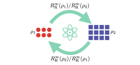
Figure 1: The second law of quantum resource theories (QRTs). Our main result, i.e., the proof of the generalized quantum Stein’s lemma, leads to an axiomatic formulation of QRTs with a second law analogous to that of thermodynamics. In this formulation, a single function, the regularized relative entropy of resource $R_{\mathrm{R}}^{\infty}$, provides the necessary and sufficient condition for the asymptotic convertibility between quantum resources (quantum states $\rho_{1}$ represented by red circles and $\rho_{2}$ by blue squares) at the optimal rate, in analogy to entropy in the second law of thermodynamics.

While thermodynamics provides a quantitative understanding of energy and entropy through the state conversion tasks, QRTs also aim to quantify the potential and limit of quantum resources. A fundamental task in QRTs is the asymptotic conversion between quantum states [2, 3], which involves converting many independently and identically distributed (IID) copies of quantum state $\rho_{1}$ into as many copies of state $\rho_{2}$ as possible with a vanishing error under the restricted operations, in the spirit of Shannon’s information theory [17, 18]. The maximum number of copies of $\rho_{2}$ obtained per $\rho_{1}$ is called the asymptotic conversion rate. In view of the success of thermodynamics, it is fundamental to seek a universal formulation of QRTs with a second law analogous to that of thermodynamics (Fig. 1). Such a second law would provide a necessary and sufficient condition for the asymptotic conversion at a certain rate characterized by a single function of $\rho_{j}$ ($j\in\{1,2\}$), similar to entropy in thermodynamics.

However, establishing the second law for QRTs has been challenging in general. In entanglement theory, for instance, the irreversibility of asymptotic state conversion under LOCC hinders the establishment of the second law to characterize the asymptotic conversion rate [19]. Nevertheless, significant progress toward the second law of entanglement theory has been made in Refs. [20, 21, 22], and this has been extended to general QRTs in Ref. [23]. Conventionally, LOCC is defined using a bottom-up approach, specifying what can be done in the laboratories. In contrast, Refs. [20, 21, 22] took a top-down approach, defining an axiomatic class of operations by specifying what cannot be done, similar to how thermodynamics axiomatically introduces adiabatic operations [10, 11, 12].

Under this class of operations, Refs. [20, 21, 22] established a remarkable connection between the asymptotic conversion of quantum states and a variant of quantum hypothesis testing [24, 25], another fundamental task in quantum information theory. This task aims to distinguish $n$ IID copies of quantum state $\rho^{\otimes n}$ from any state $\sigma_{n}$ in the set of free states, which may not be in IID form. The non-IIDness of $\sigma_{n}$ poses a substantial challenge to its analysis. References [20, 21, 22] tried to address this challenge to establish a lemma characterizing the optimal performance of this task, which is called the generalized quantum Stein’s lemma. If valid, the generalized quantum Stein’s lemma would enable a formulation of QRTs with the second law, as intended in Refs. [20, 21, 22, 23]; however, as described in Refs. [26, 27, 28, 29], a logical gap has been found in the original analysis [22] of the lemma, invalidating its consequences. Reference [29] attempted an alternative approach to resolve this issue, but their approach also turned out to be insufficient for completing the proof. Consequently, the first—and only known—general formulation of QRTs with the second law has lost its validity, reopening the question of whether such a framework can be constructed at all.

In this work, we prove the generalized quantum Stein’s lemma and reinforce the general framework for QRTs with the second law. Our proof avoids the logical gaps of the previous analyses of the generalized quantum Stein’s lemma in Refs. [22, 29] by developing alternative techniques to handle the non-IIDness based on twirling and pinching. Progressing beyond QRTs for states (static resources) in Refs. [20, 21, 22, 23], our results extend to QRTs for channels (dynamical resources) [3], encompassing existing results as a special case. Below, we will introduce the QRTs for states, present our main results on the generalized quantum Stein’s lemma, and discuss its implications for formulating QRTs with the second law, concluding with an outlook on future directions. In Methods, we detail our proof of the generalized quantum Stein’s lemma and formulate QRTs for channels with the second law.

Framework of QRTs.

We present the framework of QRTs for states based on the general formulation in Ref. [2]. We represent a quantum system by a $d$-dimensional complex Hilbert space $\mathcal{H}=\mathbb{C}^{d}$ for some finite $d$. Quantum states of $\mathcal{H}$ are positive semidefinite operators on $\mathcal{H}$ with unit trace, with the set of states of $\mathcal{H}$ denoted by $\mathcal{D}\quantity(\mathcal{H})$. For any $n\in\{1,2,\ldots\}$, a composite system of $n$ subsystems $\mathcal{H}$ is represented as $\mathcal{H}^{\otimes n}$ with tensor product. The set of quantum operations from an input system $\mathcal{H}_{\mathrm{in}}$ to an output system $\mathcal{H}_{\mathrm{out}}$ is represented by that of completely positive and trace-preserving (CPTP) linear maps (or channels), denoted by $\mathcal{C}\quantity(\mathcal{H}_{\mathrm{in}}\to\mathcal{H}_{\mathrm{out}})$.

Specifying a set of free operations defines QRTs, representing quantum operations used in quantum information processing. The set of free operations is denoted by $\mathcal{O}\quantity(\mathcal{H}_{\mathrm{in}}\to\mathcal{H}_{\mathrm{out}})\subset\mathcal{C}\quantity(\mathcal{H}_{\mathrm{in}}\to\mathcal{H}_{\mathrm{out}})$, which we may write $\mathcal{O}$ if the argument is obvious from the context. Given $\mathcal{O}$, free states are defined as states $\rho_{\mathrm{free}}$ such that for any initial state $\rho$, there exist some free operations $\mathcal{E}\in\mathcal{O}$ to convert it into $\rho_{\mathrm{free}}=\mathcal{E}\quantity(\rho)$ (in other words, regardless of how non-resourceful $\rho$ may be, $\rho_{\mathrm{free}}$ can be freely obtained, even from scratch) [2]. The set of free states of $\mathcal{H}$ is denoted by $\mathcal{F}\quantity(\mathcal{H})\subset\mathcal{D}\quantity(\mathcal{H})$. Following the previous works [20, 21, 22, 23, 29], we consider QRTs with their sets of free states satisfying the following properties.

1. The set $\mathcal{F}(\mathcal{H})$ of free states is closed and convex.

2. For each $n\in\quantity{1,2,\ldots}$, the set $\mathcal{F}(\mathcal{H}^{\otimes n})$ of free states is symmetric under permutation of $n$ subsystem; that is, if $\rho_{\mathrm{free}}\in\mathcal{F}\quantity(\mathcal{H}^{\otimes n})$, then $U(g)\rho_{\mathrm{free}}U(g)^{\dagger}\in\mathcal{F}\quantity(\mathcal{H}^{\otimes n})$ for any unitary $U(g)$ representing an element $g\in\mathfrak{S}_{n}$ of the permutation group $\mathfrak{S}_{n}$ acting on the $n$ subsystems.

3. The set of free states is closed under tensor product; that is, if $\rho_{\mathrm{free}}\in\mathcal{F}\quantity(\mathcal{H})$ and $\rho_{\mathrm{free}}^{\prime}\in\mathcal{F}\quantity(\mathcal{H}^{\prime})$, then $\rho_{\mathrm{free}}\otimes\rho_{\mathrm{free}}^{\prime}\in\mathcal{F}\quantity(\mathcal{H}\otimes\mathcal{H}^{\prime})$.

4. The set $\mathcal{F}(\mathcal{H})$ of free states contains a full-rank state $\rho_{\mathrm{full}}>0$.

Various QRTs with fundamental motivations, such as those of entanglement, athermality, coherence, asymmetry, and magic states, indeed satisfy the above properties [3]. In the original study of the generalized quantum Stein’s lemma, Refs. [20, 21] considered the entanglement theory, which has these properties. A later extension to general QRTs in Ref. [23] does not explicitly mention Property 4, but Property 4 is necessary for proving and using the generalized quantum Stein’s lemma to reproduce the results of Ref. [23]. In addition to the above properties, the existing attempts to prove the generalized quantum Stein’s lemma in Refs. [22, 29] imposed another assumption that $\mathcal{F}$ should be closed under taking the partial trace; by contrast, our proof does not impose this additional assumption, leading to broader applicability. Furthermore, whereas these properties are attributed to the free states, we also introduce their generalization to QRTs for channels. See Methods for details.

A non-free state, assisting free operations to conduct quantum information processing, is called a resource state, and QRTs provide a way to quantify such resourcefulness via resource measures. Resource measures are a family of real functions $R_{\mathcal{H}}$ of the state of every system $\mathcal{H}$ that is monotonically non-increasing under free operations; i.e., for any free operation $\mathcal{E}$ and any state $\rho$, it should hold that $R(\rho)\geq R(\mathcal{E}(\rho))$, where we may omit the subscript $\mathcal{H}$ of $R_{\mathcal{H}}$ to write $R$ if it is obvious from the context. For example, the relative entropy of resource is defined as $R_{\mathrm{R}}\quantity(\rho)\coloneqq\min_{\rho_{\mathrm{free}}\in\mathcal{F}\quantity(\mathcal{H})}D\left(\rho\middle|\middle|\rho_{\mathrm{free}}\right)$ [3, 2], where $D\left(\rho\middle|\middle|\sigma\right)\coloneqq\Tr[\rho(\log\rho-\log\sigma)]$ is the quantum relative entropy, and $\log$ is the natural logarithm throughout this work. Its variant, the regularized relative entropy of resources, is defined as $R_{\mathrm{R}}^{\infty}\quantity(\rho)\coloneqq\lim_{n\to\infty}\frac{1}{n}R_{\mathrm{R}}\quantity(\rho^{\otimes n})$ [3, 2]. Another example is the generalized robustness of resource (also known as global robustness) defined as $R_{\mathrm{G}}\quantity(\rho)\coloneqq\min\quantity{s\geq 0:\frac{\rho+s\rho^{\prime}}{1+s}\in\mathcal{F}(\mathcal{H}),\rho^{\prime}\in\mathcal{D}\quantity(\mathcal{H})}$ [3]. All these $R_{\mathrm{R}}$, $R_{\mathrm{R}}^{\infty}$, and $R_{\mathrm{G}}$ serve as resource measures, satisfying the monotonicity as required [3].

A fundamental task in QRTs is the asymptotic conversion of quantum states. This task involves converting many copies of one state, $\rho_{1}$, into as many copies as possible of another state, $\rho_{2}$, using free operations, within errors that vanish asymptotically. The conversion rate $r_{\mathcal{O}}\quantity(\rho_{1}\to\rho_{2})$, under a class $\mathcal{O}$ of operations, is the supremum of achievable rates $r$ in this asymptotic conversion. Specifically, $r$ is achievable if $\liminf_{n\to\infty}\frac{1}{2}\left\|\mathcal{E}_{n}\quantity(\rho_{1}^{\otimes n})-\rho_{2}^{\otimes\lceil rn\rceil}\right\|_{1}=0$ for some sequence $\{\mathcal{E}_{n}\}_{n}$ of operations in $\mathcal{O}$, where $\lceil{}\cdots{}\rceil$ is the ceiling function, and $\|\cdots\|_{1}$ is the trace norm [2]. For example, in the entanglement theory, $\mathcal{O}$ can be chosen as LOCC, making $\mathcal{F}$ the set of separable states [2, 3]. However, under such $\mathcal{O}$, $r_{\mathcal{O}}\quantity(\rho_{1}\to\rho_{2})$ cannot be characterized by a single resource measure $R$ due to the irreversibility of conversion between mixed entangled states [19, 30, 31]. To address this issue, as in the previous works [20, 21, 22, 23], one can consider a slightly broader, axiomatically defined class of operations, $\tilde{\mathcal{O}}$, as a relaxation of $\mathcal{O}$. A fundamental question in QRTs is whether it is possible to establish a general framework of QRTs with an appropriate choice of the class $\tilde{\mathcal{O}}$ of operations and a single resource measure $R$ such that the resource measures $R(\rho_{j})$ ($j\in\{1,2\}$) characterize the convertibility at rate $r_{\tilde{\mathcal{O}}}\quantity(\rho_{1}\to\rho_{2})$, which would constitute the second law of QRTs.

Main result: Generalized quantum Stein’s lemma.

— For establishing such a desired framework of QRTs, the generalized quantum Stein’s lemma plays a crucial role, characterizing the optimal performance of a variant of quantum hypothesis testing; our main result is proof of the generalized quantum Stein’s lemma. In this variant of quantum hypothesis testing, as introduced in Ref. [22], we are initially given $n\in\{1,2,\ldots\}$, a classical description of a state $\rho$ of $\mathcal{H}$, and an unknown quantum state of $\mathcal{H}^{\otimes n}$. The task is to perform a two-outcome measurement by a positive operator-valued measure (POVM) $\{T_{n},\mathds{1}-T_{n}\}$ on $\mathcal{H}^{\otimes n}$ (where $\mathds{1}$ is the identity operator, and $0\leq T_{n}\leq\mathds{1}$) to distinguish the following two cases.

• Null hypothesis: The given unknown state is $n$ IID copies $\rho^{\otimes n}$ of $\rho$.

• Alternative hypothesis: The given state is some free state $\sigma\in\mathcal{F}\quantity(\mathcal{H}^{\otimes n})$ in the set satisfying Properties 1–4, where $\sigma$ may have a non-IID form over $\mathcal{H}^{\otimes n}$.

If the measurement outcome is $T_{n}$, we conclude that the given state was $\rho^{\otimes n}$, and if $\mathds{1}-T_{n}$, then was some free state $\sigma\in\mathcal{F}\quantity(\mathcal{H}^{\otimes n})$. For this hypothesis testing, we define the following two types of errors.

• Type I error: The mistaken conclusion that the given state was some free state $\sigma\in\mathcal{F}\quantity(\mathcal{H}^{\otimes n})$ when it was $\rho^{\otimes n}$, which happens with probability $\alpha_{n}\coloneqq\Tr\quantity[\quantity(\mathds{1}-T_{n})\rho^{\otimes n})]$.

• Type II error: The mistaken conclusion that the given state was $\rho^{\otimes n}$ when it was some free state $\sigma\in\mathcal{F}\quantity(\mathcal{H}^{\otimes n})$, which happens with probability $\beta_{n}\coloneqq\max_{\sigma\in\mathcal{F}(\mathcal{H}^{\otimes n})}\Tr\quantity[T_{n}\sigma]$ in the worst case.

For any target type I error $\epsilon\in(0,1)$, by choosing appropriate POVMs, we can suppress the type II error exponentially in $n$ while keeping the type I error below $\epsilon$; as shown below, the generalized quantum Stein’s lemma characterizes the optimal exponent, i.e., the fastest rate in suppressing the type II error, by the regularized relative entropy of resource. Note that by choosing $\mathcal{F}\quantity(\mathcal{H}^{\otimes n})=\quantity{\sigma^{\otimes n}}$, the generalized quantum Stein’s lemma reduces to quantum Stein’s lemma for quantum hypothesis testing in the conventional setting [24, 25, 22]. See Methods for the details of our proof.

Theorem 1 (Generalized quantum Stein’s lemma).

Given any family $\mathcal{F}$ of sets of states satisfying Properties 1–4, any state $\rho$ of $\mathcal{H}$, and any target type I error $\epsilon\in(0,1)$, the optimal exponent of type II error is

$$\lim_{n\to\infty}-\frac{\log\quantity(\min_{T_{n}}\max_{\sigma\in\mathcal{F}\quantity(\mathcal{H}^{\otimes n})}\Tr\quantity[T_{n}\sigma])}{n}=R_{\mathrm{R}}^{\infty}(\rho),$$ (1)

where the minimum is taken over all POVMs $\quantity{T_{n},\mathds{1}-T_{n}}$ suppressing the type I error below $\epsilon$, i.e., $\Tr[\quantity(\mathds{1}-T_{n})\rho^{\otimes n}]\leq\epsilon$, and $R_{\mathrm{R}}^{\infty}$ is the regularized relative entropy of resource.

The challenge in the proof of Theorem 1 arises from the non-IIDness of $\sigma\in\mathcal{F}\quantity(\mathcal{H}^{\otimes n})$. To address the non-IIDness, Ref. [22] considered using the symmetry of this task under the permutation of the $n$ subsystems. This symmetry implies that almost all states of the $n$ subsystems are virtually identical and independent of each other [32, 33], approximately recovering the IID structure of the state. Then, Ref. [22] tried to show that this approximation for recovering the IID structure would not change the quantum relative entropy up to a negligibly small amount, so the optimal exponent would coincide with its regularization $R_{\mathrm{R}}^{\infty}(\rho)$ if Lemma III.9 of Ref. [22] were true, where the logical gap of the proof was found [26]. Reference [29] also tried to address this non-IIDness using a continuity bound in the second argument of the quantum relative entropy in Refs. [34, 35], but it turned out that these continuity bounds are not tight enough for completing the proof. By contrast, our proof overcomes the non-IIDness by developing alternative techniques based on twirling under the permutation group, which allows us to use a pinching technique to maintain the commutativity of operators in the core part of our analysis. See Methods for details.

The second law of QRTs.

Our proof of the generalized quantum Stein’s lemma leads to the second law of QRTs, as originally intended in Refs. [20, 21, 22, 23]. So far, we have introduced the class $\mathcal{O}$ of free operations in a conventional way, i.e., in a bottom-up approach by specifying what can be done. By contrast, Refs. [20, 21, 22, 23] formulated QRTs by introducing a slightly broader class $\tilde{O}$ of operations defined in an axiomatic approach by specifying what cannot be done, as in the adiabatic operations in thermodynamics.

A fundamental requirement for free operations $\mathcal{O}$ is that the free operations should not generate resource states from free states; however, in the context of asymptotic conversion, it is possible to axiomatically define a relaxed class of operations, $\tilde{O}$, which captures this requirement only in an asymptotic sense. Various axiomatic definitions of $\tilde{O}$ can be considered, but even with such $\tilde{O}$, formulating general QRTs with the second law remains highly challenging [31, 30]. The second law does hold for special types of quantum resources, such as QRTs of coherence [36, 37, 26] and athermality [38, 39]; similarly, formulating QRTs with the second law may be possible using some variants of composite quantum Stein’s lemmas [40, 41, 42, 43], but these formulations are not general enough to cover entanglement [26]. Theories with the second law can also be developed by considering “operations” that extend beyond the limitations of quantum mechanics, such as allowing post-selection [44], non-physical quasi-operations [45], and the use of batteries [46]. However, to maintain full generality within the law of quantum mechanics, the only known approach to introducing $\tilde{O}$ that leads to QRTs with the second law is based on the generalized quantum Stein’s lemma, as originally attempted Refs. [20, 21, 22, 23]. Following Refs. [20, 21, 22, 23], we define a class $\tilde{O}$ of asymptotically resource-non-generating operations as a sequence $\tilde{\mathcal{O}}\quantity(\mathcal{H}_{\mathrm{in}}\to\mathcal{H}_{\mathrm{out}})\coloneqq\quantity{\tilde{\mathcal{O}}_{n}\subset\mathcal{C}\quantity(\mathcal{H}_{\mathrm{in}}^{\otimes n}\to\mathcal{H}_{\mathrm{out}}^{\otimes n})}_{n}$ of the sets of operations (CPTP linear maps) such that any sequence of operations in these sets asymptotically generates no resource from any free states in terms of the generalized robustness of resource $R_{\mathrm{G}}$, i.e.,

$$\lim_{n\to\infty}\max_{\begin{subarray}{c}\mathcal{E}_{n}\in\tilde{\mathcal{O}}_{n}\\ \rho_{\mathrm{free}}^{(n)}\in\mathcal{F}\quantity(\mathcal{H}_{\mathrm{in}}^{\otimes n})\end{subarray}}R_{\mathrm{G}}\quantity(\mathcal{E}_{n}\quantity(\rho_{\mathrm{free}}^{(n)}))=0.$$ (2)

Under $\tilde{\mathcal{O}}$ satisfying (2), using the generalized quantum Stein’s lemma in Theorem 1, we show a characterization of the asymptotic convertibility of resource states, as stated by the theorem below. We also extend this theorem from the static resource of states to the dynamical resource of channels, as presented in Methods in detail.

Theorem 2 (Second law of QRTs for states).

Given any family $\mathcal{F}$ of sets of free states satisfying Properties 1–4, for any states $\rho_{1}$ and $\rho_{2}$ satisfying $R_{\mathrm{R}}^{\infty}(\rho_{j})>0$ ($j\in\{1,2\}$), the asymptotic conversion rate between $\rho_{1}$ and $\rho_{2}$ under the asymptotically resource-non-generating operations $\tilde{\mathcal{O}}$ satisfying (2) is

$$r_{\tilde{\mathcal{O}}}\quantity(\rho_{1}\to\rho_{2})=\frac{R_{\mathrm{R}}^{\infty}\quantity(\rho_{1})}{R_{\mathrm{R}}^{\infty}\quantity(\rho_{2})}.$$ (3)

To prove Theorem 2, assuming the generalized quantum Stein’s lemma, Ref. [23] originally showed an inequality $r_{\tilde{\mathcal{O}}}\quantity(\rho_{1}\to\rho_{2})\geq\frac{R_{\mathrm{R}}^{\infty}\quantity(\rho_{1})}{R_{\mathrm{R}}^{\infty}\quantity(\rho_{2})}$ in QRTs for states. The proof of the opposite inequality $r_{\tilde{\mathcal{O}}}\quantity(\rho_{1}\to\rho_{2})\leq\frac{R_{\mathrm{R}}^{\infty}\quantity(\rho_{1})}{R_{\mathrm{R}}^{\infty}\quantity(\rho_{2})}$ was not discussed in Ref. [23] but later provided in Ref. [44] with an extension to probabilistic protocols. Our contribution is to prove both directions of these inequalities in a more general framework of QRTs for channels, which includes Theorem 2 in QRTs for states as a special case. We emphasize that this generalization involves identifying nontrivial conditions for $\tilde{O}$ in QRTs for channels, as was done for QRTs for states in Refs. [20, 21, 22, 23]. See Methods for details.

The equation (3) represents the second law of QRTs. This is analogous to the axiomatic formulation of the second law of thermodynamics in Refs. [10, 11, 12], which provides the necessary and sufficient condition for convertibility between thermodynamic states $X_{1}$ and $X_{2}$ under adiabatic operations solely by comparing the (additive) entropy functions $S(X_{1})$ and $S(X_{2})$. In the framework of QRTs described by Theorem 2, the regularized relative entropy of resource $R_{\mathrm{R}}^{\infty}$ takes the role of entropy in thermodynamics. Similar to the idealization of quasi-static processes under adiabatic operations, which are axiomatically introduced in thermodynamics [10, 11, 12] and may not be exactly realizable in practice, it may be generally unknown how to realize all operations in the axiomatically defined class $\tilde{O}$. However, this axiomatic class of operations is broad enough to include all physically realizable operations, ensuring its universal applicability regardless of future technological advances, much like thermodynamics.

Lastly, for instance in the entanglement theory, $\mathcal{F}(\mathcal{H})$ is taken as the set of separable states on two spatially separated systems $A$ and $B$ [4], and a fundamental resource state is an ebit, i.e., $\Phi_{2}\coloneqq\ket{\Phi_{2}}\bra{\Phi_{2}}$ with $\ket{\Phi_{2}}\coloneqq\frac{1}{\sqrt{2}}\quantity(\ket{0}^{A}\otimes\ket{0}^{B}+\ket{1}^{A}\otimes\ket{1}^{B})$. For an ebit, we have $R_{\mathrm{R}}^{\infty}\quantity(\Phi_{2})=1$ [4]. In the asymptotic conversion from any state $\rho$ to ebit $\Phi_{2}$, the maximum number of ebits $\Phi_{2}$ obtained per $\rho$ is called the distillable entanglement [47], written under the class $\tilde{O}$ of operations as $E_{\mathrm{D},\tilde{\mathcal{O}}}(\rho)\coloneqq r_{\tilde{\mathcal{O}}}\quantity(\rho\to\Phi_{2})$. Also in the asymptotic conversion rate from $\Phi_{2}$ to $\rho$, the minimum required number of ebits $\Phi_{2}$ per $\rho$ is called the entanglement cost [47, 48, 6], which is given under $\tilde{\mathcal{O}}$ by $E_{\mathrm{C},\tilde{\mathcal{O}}}(\rho)\coloneqq 1/{r_{\tilde{\mathcal{O}}}\quantity(\Phi_{2}\to\rho)}$ [2]. Due to (3), our results establish the asymptotic reversibility between all, pure and mixed, bipartite entangled states, as originally intended in Refs. [20, 21], i.e., $E_{\mathrm{D},\tilde{\mathcal{O}}}(\rho)=E_{\mathrm{C},\tilde{\mathcal{O}}}(\rho)=R_{\mathrm{R}}^{\infty}(\rho)$, which resolves the question of the possibility of formulating the reversible framework of entanglement theory raised in Ref. [49]. See also Methods for other examples.

Outlook.

In this work, we proved the generalized quantum Stein’s lemma (Theorem 1), resolving a fundamental open problem in quantum information theory by overcoming the logical gaps of the existing analyses in Refs. [22, 29]. Our proof enables the formulation of the framework of QRTs equipped with the second law under Properties 1–4 (Theorem 2), as originally intended in Refs. [20, 21, 22, 23]. In this framework, a single resource measure, the regularized relative entropy of resource, characterizes the asymptotic convertibility between resource states at the optimal rate, analogous to entropy in the second law of thermodynamics. Since the publication of the initial works [20, 21, 22, 23], the scope of QRTs has expanded far beyond entanglement [3, 2]; therefore, we also extend the framework of QRTs with the second law from those for states to those for channels, broadening their applicability (see Methods for details). A remaining open question is how universally our results further generalize beyond convex and finite-dimensional QRTs satisfying Properties 1–4, for example, to non-convex QRTs [2, 50, 51, 52] and infinite-dimensional QRTs [2, 50, 53, 54, 55, 6]. The generalized quantum Stein’s lemma itself also serves as a valuable tool for analysis in quantum information theory, such as examining the faithfulness of the regularized relative entropy of entanglement [56, 22] and the squashed entanglement [26, 57]. Exploring further applications of this lemma would also be an intriguing research direction. Given the success of thermodynamics, these general results are expected to be fundamental in studying the vast possibilities of the use of quantum resources in the future.

Author contributions

Both authors contributed to the conception of the work, the analysis and interpretation of the work, and the preparation of the manuscript.

Competing interests

The authors declare no competing interests.

Additional information

Supplementary Information is available for this paper. Correspondence and requests for materials should be addressed to Masahito Hayashi and Hayata Yamasaki.

Methods

Proof of generalized quantum Stein’s lemma

We analyze the task of quantum hypothesis testing presented in the main text. We have two possible states $\rho$ and $\sigma$ on a given physical system ${\cal H}$ as our two hypotheses. The performance of the discrimination between these two hypotheses is characterized by

$$\beta_{\epsilon}(\rho\|\sigma)\coloneqq\min_{T:0\leq T\leq\mathds{1}}\{\Tr[T\sigma]:\Tr[(\mathds{1}-T)\rho]\leq\epsilon\},$$ (4)

where $\mathds{1}$ is the identity operator. In the setting of generalized quantum Stein’s lemma, we consider the case when one hypothesis is given as a convex set ${\cal S}$ of states on the system ${\cal H}$. Such a hypothesis is called a composite hypothesis. In this case, the performance is characterized by

$$\beta_{\epsilon}\left(\rho\middle\|{\cal S}\right)\coloneqq\min_{T:0\leq T\leq\mathds{1}}\max_{\sigma\in{\cal S}}\quantity{\Tr[T\sigma]:\Tr[(\mathds{1}-T)\rho]\leq\epsilon}.$$ (5)

Generally, these two quantities satisfy the max-min inequality

$$\max_{\sigma\in{\cal S}}\beta_{\epsilon}\left(\rho\middle\|\sigma\right)\leq\beta_{\epsilon}\left(\rho\middle\|{\cal S}\right).$$ (6)

Interestingly, as shown in Section I, these two quantities have the following relation when $\mathcal{S}$ is convex.

Lemma 3.

For any convex set ${\cal S}$ and any $\epsilon>0$, we have

$$\max_{\sigma\in{\cal S}}\beta_{\epsilon}\left(\rho\middle\|\sigma\right)=\beta_{\epsilon}\left(\rho\middle\|{\cal S}\right).$$ (7)

To characterize these quantities, we consider the $n$-fold tensor product system ${\cal H}^{\otimes n}$ composed of a $d$-dimensional subsystem ${\cal H}$. In this system, we may consider $n$-fold tensor product states $\rho^{\otimes n}$ and $\sigma^{\otimes n}$. Then, due to the quantum Stein’s lemma, for any $\epsilon\in(0,1)$, we have the relation [24, 25]

$$\lim_{n\to\infty}-\frac{1}{n}\log\beta_{\epsilon}\left(\rho^{\otimes n}\middle\|\sigma^{\otimes n}\right)=D\left(\rho\middle\|\sigma\right),$$ (8)

where $D(\rho\|\sigma)\coloneqq\Tr[\rho(\log\rho-\log\sigma)]$ is the quantum relative entropy, and the function $\log$ is the natural logarithm throughout this work. As its natural extension to the composite hypothesis, for a sequence of convex sets ${\cal S}_{n}$ of states of ${\cal H}^{\otimes n}$, one may consider the relation between $\lim_{n\to\infty}-\frac{1}{n}\log\beta_{\epsilon}\left(\rho^{\otimes n}\middle\|{\cal S}_{n}\right)$ (=$\lim_{n\to\infty}-\frac{1}{n}\log\max_{\sigma\in{\cal S}_{n}}\beta_{\epsilon}\left(\rho^{\otimes n}\middle\|\sigma\right)$) and $\lim_{n\to\infty}\frac{1}{n}\min_{\sigma\in{\cal S}_{n}}D\left(\rho^{\otimes n}\middle\|\sigma\right)$. In contrast to Lemma 5, it is not clear whether these quantities are equal in general. To address this problem, we denote the set of permutation on $\{1,\ldots,n\}$ by $\mathfrak{S}_{n}$, and denote the unitary operator of the permutation operation $g\in\mathfrak{S}_{n}$ for the order of the tensor product by $U(g)$. Then, as in the conditions for the set of free states in the main text, we introduce the following conditions for ${\cal S}_{n}$:

(a)

${\cal S}_{n}$ is a convex closed set;

(b)

${\cal S}_{n}$ is closed for the application of permutation group $\mathfrak{S}_{n}$ for the order of tensor product;

(c)

if $\sigma_{n}\in{\cal S}_{n}$ and $\sigma_{m}\in{\cal S}_{m}$, then $\sigma_{n}\otimes\sigma_{m}\in{\cal S}_{n+m}$ for any positive integers $n$ and $m$;

(d)

${\cal S}_{1}$ contains a state $\sigma_{\mathrm{full}}$ with full support, where we write the minimum eigenvalue of $\sigma_{\mathrm{full}}$ by $e^{-\lambda}$.

Our main result is stated as follows.

Theorem 4 (Generalized quantum Stein’s lemma).

If a sequence $\quantity{{\cal S}_{n}}_{n}$ of sets satisfies conditions (a), (b), (c), and (d), then for any $\epsilon\in(0,1)$, it holds that

$$\lim_{n\to\infty}-\frac{1}{n}\log\beta_{\epsilon}\left(\rho^{\otimes n}\middle\|{\cal S}_{n}\right)=\lim_{n\to\infty}\frac{1}{n}\min_{\sigma\in{\cal S}_{n}}D\left(\rho^{\otimes n}\middle\|\sigma\right).$$ (9)

As presented in the main text, the difficulty of proving (9) stems from the complicated structure of the set ${\cal S}_{n}$. To avoid the difficulty, we employ a smaller set

$${\cal S}_{n,\mathop{\rm sym}}\coloneqq \quantity{\sigma\in{\cal S}_{n}:U(g)\sigma U(g)^{\dagger}=\sigma,~{}g\in\mathfrak{S}_{n}}.$$ (10)

The set ${\cal S}_{n,\mathop{\rm sym}}$ of permutation-invariant states still satisfies the convexity. As shown in Section II, the quantities in (9) are characterized by the set ${\cal S}_{n,\mathop{\rm sym}}$ as follows.

Lemma 5.

When a sequence of sets ${\cal S}_{n}$ satisfies condition (a) and (b), for any $\epsilon\geq 0$, we have

$$\beta_{\epsilon}\left(\rho^{\otimes n}\middle\|{\cal S}_{n}\right) =\beta_{\epsilon}\left(\rho^{\otimes n}\middle\|{\cal S}_{n,\mathop{\rm sym}}\right),$$ (11)

$$\max_{\sigma\in{\cal S}_{n}}\beta_{\epsilon}\left(\rho^{\otimes n}\middle\|\sigma\right) =\max_{\sigma\in{\cal S}_{n,\mathop{\rm sym}}}\beta_{\epsilon}\left(\rho^{\otimes n}\middle\|\sigma\right),$$ (12)

$$\min_{\sigma\in{\cal S}_{n}}D\left(\rho^{\otimes n}\middle\|\sigma\right) =\min_{\sigma\in{\cal S}_{n,\mathop{\rm sym}}}D\left(\rho^{\otimes n}\middle\|\sigma\right).$$ (13)

Also, as shown in Section III, we have the following lemma.

Lemma 6.

When a sequence of sets ${\cal S}_{n}$ satisfies conditions (a), (b), and (c), the limits

$$\lim_{n\to\infty}\frac{1}{n}\min_{\sigma\in{\cal S}_{n}}D\left(\rho^{\otimes n}\middle\|\sigma\right)~{}\text{and}$$ (14)

$$\lim_{n\to\infty}\frac{1}{n}\min_{\sigma\in{\cal S}_{n,\mathop{\rm sym}}}D\left(\rho^{\otimes n}\middle\|\sigma\right)$$ (15)

exist.

Due to Lemmas 3, 5, and 6, it suffices to deal with $\max_{\sigma\in{\cal S}_{n,\mathop{\rm sym}}}\beta_{\epsilon}\left(\rho^{\otimes n}\middle\|\sigma\right)$ and $\min_{\sigma\in{\cal S}_{n,\mathop{\rm sym}}}D\left(\rho^{\otimes n}\middle\|\sigma\right)$; in particular, our strategy focuses on analyzing the following relation instead of (9):

$$\lim_{n\to\infty}-\frac{1}{n}\log\max_{\sigma\in{\cal S}_{n,\mathop{\rm sym}}}\beta_{\epsilon}\left(\rho^{\otimes n}\middle\|\sigma\right)$$

$$=\lim_{n\to\infty}\frac{1}{n}\min_{\sigma\in{\cal S}_{n,\mathop{\rm sym}}}D\left(\rho^{\otimes n}\middle\|\sigma\right).$$ (16)

To show an inequality $\leq$ in (16), i.e., the strong converse part, we employ the following lemma, which is shown in Section IV by a modification of the standard proof of the strong converse of quantum Stein’s lemma [25].

Lemma 7.

Given any fixed positive integer $m$, any state $\rho$ of ${\cal H}$, and any state $\sigma_{m}$ of ${\cal H}^{\otimes m}$, for each $n$ (with $k$ satisfying $km\leq n<(k+1)m$), we define states

$$\tilde{\sigma}_{n}^{\ast}\coloneqq\sigma_{m}^{\otimes k}\otimes\sigma_{\mathrm{full}}^{\otimes(n-km)},$$ (17)

where $\sigma_{\mathrm{full}}$ is the full-rank state in $\mathcal{S}_{1}$. For any $\epsilon\in[0,1)$, we have

$$\limsup_{n\to\infty}-\frac{1}{n}\log\beta_{\epsilon}\left(\rho^{\otimes n}\middle\|\tilde{\sigma}_{n}^{\ast}\right)\leq\frac{1}{m}D\left(\rho^{\otimes m}\middle\|\sigma_{m}\right).$$ (18)

By choosing $\sigma_{m}\in{\cal S}_{m}$ in Lemma 7, we have

$$\limsup_{n\to\infty}-\frac{1}{n}\max_{\sigma\in{\cal S}_{n}}\log\beta_{\epsilon}\left(\rho^{\otimes n}\middle\|\sigma\right)$$

$$\leq\limsup_{n\to\infty}-\frac{1}{n}\log\beta_{\epsilon}\left(\rho^{\otimes n}\middle\|\tilde{\sigma}_{n}^{\ast}\right)\leq\frac{1}{m}D\left(\rho^{\otimes m}\middle\|\sigma_{m}\right),$$ (19)

which holds for any $m$ and $\epsilon\in[0,1)$. Therefore, by choosing $\sigma_{m}$ as that minimizing $\min_{\sigma\in\mathcal{S}_{n,\mathop{\rm sym}}}D\left(\rho^{\otimes m}\middle\|\sigma\right)$ and taking $m\to\infty$, Lemmas 5, 6, and 7 lead to

$$\limsup_{n\to\infty}-\frac{1}{n}\max_{\sigma\in{\cal S}_{n,\mathop{\rm sym}}}\log\beta_{\epsilon}\left(\rho^{\otimes n}\middle\|\sigma\right)$$

$$\leq\lim_{m\to\infty}\frac{1}{m}D\left(\rho^{\otimes m}\middle\|\sigma_{m}\right)$$ (20)

$$=\lim_{n\to\infty}\frac{1}{n}\min_{\sigma\in{\cal S}_{n,\mathop{\rm sym}}}D\left(\rho^{\otimes n}\middle\|\sigma\right),$$ (21)

which shows the inequality $\leq$ in (16) for any $\epsilon\in[0,1)$. Thus, recalling that $\epsilon>0$ in Lemma 3, we see that the inequality $\leq$ in (9) has been shown for any $\epsilon\in(0,1)$.

Therefore, the key part of the generalized quantum Stein’s lemma is the proof of the opposite inequality $\geq$ in (16), i.e., the direct part. For any $\epsilon\in(0,1)$, with

$$R_{1,\epsilon}\coloneqq\liminf_{n\to\infty}-\frac{1}{n}\max_{\sigma\in{\cal S}_{n,\mathop{\rm sym}}}\log\beta_{\epsilon}\left(\rho^{\otimes n}\middle\|\sigma\right),$$ (22)

the goal of our analysis is to find a sequence $\quantity{\sigma_{n,*}\in{\cal S}_{n,\mathop{\rm sym}}}_{n}$ of states of ${\cal H}^{\otimes n}$ such that

$$R_{1,\epsilon}\geq\liminf_{n\to\infty}\frac{1}{n}D\left(\rho^{\otimes n}\middle\|\sigma_{n,*}\right).$$ (23)

Then, (23) implies that, for any $\epsilon\in(0,1)$,

$$\liminf_{n\to\infty}-\frac{1}{n}\max_{\sigma\in{\cal S}_{n,\mathop{\rm sym}}}\log\beta_{\epsilon}\left(\rho^{\otimes n}\middle\|\sigma\right)$$

$$\geq\lim_{n\to\infty}\frac{1}{n}\min_{\sigma\in{\cal S}_{n,\mathop{\rm sym}}}D\left(\rho^{\otimes n}\middle\|\sigma\right).$$ (24)

The combination of (21) and (24) completes the proof of (16) and thus (9) for any $\epsilon\in(0,1)$.

To seek $\sigma_{n_{k},*}$ in (23), we prepare the following lemma, which is shown in Section V.

Lemma 8.

Given any sequence $\quantity{\sigma_{n}\in{\cal S}_{n,\mathop{\rm sym}}}_{n}$ of states, suppose that

$$R_{2}\coloneqq\liminf_{n\to\infty}\frac{1}{n}D\left(\rho^{\otimes n}\middle\|\sigma_{n}\right)\geq R_{1,\epsilon},$$ (25)

where $R_{1,\epsilon}$ is defined as (22) for any $\epsilon\in(0,1)$. Then, for any fixed parameter $\tilde{\epsilon}\in(0,\epsilon)$, there exists a sequence $\quantity{\sigma_{n}^{\prime}\in{\cal S}_{n,\mathop{\rm sym}}}_{n}$ of states such that

$$\liminf_{n\to\infty}\frac{1}{n}D\left(\rho^{\otimes n}\middle\|\sigma_{n}^{\prime}\right)-R_{1,\epsilon} \leq(1-\tilde{\epsilon})(R_{2}-R_{1,\epsilon}).$$ (26)

Given $R_{1,\epsilon}$ in (22), we start with any sequence $\quantity{\sigma_{n}\in{\cal S}_{n,\mathop{\rm sym}}}_{n}$ and apply Lemma 8 to obtain an updated sequence $\quantity{\sigma_{n,1}}_{n}$ satisfying

$$\liminf_{n\to\infty}\frac{1}{n}D\left(\rho^{\otimes n}\middle\|\sigma_{n,1}\right)-R_{1,\epsilon} \leq(1-\tilde{\epsilon})(R_{2}-R_{1,\epsilon}).$$ (27)

Applying Lemma 8 twice, we obtain a sequence $\quantity{\sigma_{n,2}}_{n}$ satisfying

$$\liminf_{n\to\infty}\frac{1}{n}D\left(\rho^{\otimes n}\middle\|\sigma_{n,2}\right)-R_{1,\epsilon} \leq(1-\tilde{\epsilon})^{2}(R_{2}-R_{1,\epsilon}).$$ (28)

When Lemma 8 is applied $k$ times, there exists a sequence $\quantity{\sigma_{n,k}}_{n}$ to satisfy

$$\liminf_{n\to\infty}\frac{1}{n}D\left(\rho^{\otimes n}\middle\|\sigma_{n,k}\right)-R_{1,\epsilon} \leq(1-\tilde{\epsilon})^{k}(R_{2}-R_{1,\epsilon}).$$ (29)

Due to (29), for any vanishing sequence $\{\epsilon_{k}>0\}_{k}$ ($\lim_{k\to\infty}\epsilon_{k}=0$), there exists a subsequence $\{n_{k}\}_{k}$ such that for all $k$

$$\frac{1}{n_{k}}D\left(\rho^{\otimes n_{k}}\middle\|\sigma_{n_{k},k}\right)-R_{1,\epsilon} \leq(1-\tilde{\epsilon})^{k}(R_{2}-R_{1,\epsilon})+\epsilon_{k}$$ (30)

$$\to 0\quad\text{as $k\to\infty$}.$$ (31)

Therefore, a sequence $\{\sigma_{n,*}\}_{n}$ such that $\sigma_{n_{k},*}=\sigma_{n_{k},k}$ for all $k$ satisfies (23).

Finally, we sketch the proof of Lemma 8, which requires our key techniques for addressing the non-IIDness. When $R_{2}=R_{1,\epsilon}$, the statement is trivial. Hence, we assume that $R_{2}>R_{1,\epsilon}$. In our proof, the twirling ${\cal W}_{\mathfrak{S}_{n}}$ plays a key role, defined as

$${\cal W}_{\mathfrak{S}_{n}}(\sigma) \coloneqq\sum_{g\in\mathfrak{S}_{n}}\frac{1}{n!}U(g)\sigma U(g)^{\dagger}.$$ (32)

Fix a parameter

$$\epsilon_{0}\coloneqq\frac{\epsilon-\tilde{\epsilon}}{1-\epsilon}\quantity(R_{2}-R_{1,\epsilon}).$$ (33)

For this fixed $\epsilon_{0}$, we choose a fixed integer $m$ such that

$$\frac{1}{m}D\left(\rho^{\otimes m}\middle\|\sigma_{m}\right)\leq R_{2}+\epsilon_{0}.$$ (34)

Then, using the states $\sigma_{n}^{\ast}\coloneqq\mathop{\rm argmax}_{\sigma\in{\cal S}_{n,\mathop{\rm sym}}}\beta_{\epsilon}\left(\rho^{\otimes n}\middle\|\sigma\right)$ and $\tilde{\sigma}_{n}^{\ast}\coloneqq\sigma_{m}^{\otimes k}\otimes\sigma_{\mathrm{full}}^{\otimes(n-mk)}$ (as in Lemma 7, where $k$ is the integer satisfying $mk\leq n<m(k+1)$), we construct

$$\sigma_{n}^{\prime}\coloneqq\frac{1}{3}\quantity(\sigma_{n}^{\ast}+{\cal W}_{\mathfrak{S}_{n}}\quantity(\tilde{\sigma}_{n}^{\ast})+\sigma_{\mathrm{full}}^{\otimes n}),$$ (35)

where $\sigma_{\mathrm{full}}$ is the full-rank state in $\mathcal{S}_{1}$. Since the state ${\cal W}_{\mathfrak{S}_{n}}(\tilde{\sigma}_{n}^{\ast})$ is permutation-invariant, the state $\sigma_{n}^{\prime}$ as well; i.e., $\sigma_{n}^{\prime}\in\mathcal{S}_{n,\mathop{\rm sym}}$.

We then introduce a pinching map ${\cal E}_{n}$ with respect to the state $\sigma_{n}^{\prime}$; that is, we write the spectral decomposition of $\sigma_{n}^{\prime}$ as $\sum_{j}\lambda_{j}E_{j}$, so ${\cal E}_{n}$ is defined as

$${\cal E}_{n}(\sigma)\coloneqq\sum_{j}E_{j}\sigma E_{j}.$$ (36)

Due to the permutation invariance of the state $\sigma_{n}^{\prime}$, we can show that the number of projections $E_{j}$ is upper bounded by a polynomial factor $v_{n}\coloneqq(n+1)^{(d+2)(d-1)/2}$ in $n$. Using the fact that $D\left(\rho^{\otimes n}\middle\|\mathcal{E}_{n}\quantity(\rho^{\otimes n})\right)\leq\log v_{n}=o(n)$, we can show

$$\liminf_{n\to\infty}\frac{1}{n}D\left(\rho^{\otimes n}\middle\|\sigma_{n}^{\prime}\right)=\liminf_{n\to\infty}\frac{1}{n}D({\cal E}_{n}\left(\rho^{\otimes n})\middle\|\sigma_{n}^{\prime}\right).$$ (37)

Then, (26) will follow from the relation

$$\liminf_{n\to\infty}\frac{1}{n}D\left({\cal E}_{n}(\rho^{\otimes n})\middle\|\sigma_{n}^{\prime}\right)-R_{1,\epsilon} \leq(1-\tilde{\epsilon})(R_{2}-R_{1,\epsilon}),$$ (38)

where, importantly, ${\cal E}_{n}(\rho^{\otimes n})$ and $\sigma_{n}^{\prime}$ commute due to the pinching.

To prove (38), for any $\epsilon_{1}\in(0,1]$, we show in Section V the relations

$$\limsup_{n\to\infty}-\frac{1}{n}\log\beta_{1-\epsilon_{1}}\left({\cal E}_{n}(\rho^{\otimes n})\middle\|\sigma_{n}^{\prime}\right) \leq\frac{1}{m}D\left(\rho^{\otimes m}\middle\|\sigma_{m}\right)$$

$$\leq R_{2}+\epsilon_{0},$$ (39)

$$\liminf_{n\to\infty}-\frac{1}{n}\log\beta_{\epsilon}({\cal E}_{n}\left(\rho^{\otimes n})\middle\|\sigma_{n}^{\prime}\right) \leq R_{1,\epsilon}.$$ (40)

For any $\epsilon_{2}>0$, we then define two projections

$$P_{n,1} \coloneqq\quantity{{\cal E}_{n}\quantity(\rho^{\otimes n})\leq e^{n(R_{2}+\epsilon_{0}+\epsilon_{2})}\sigma_{n}^{\prime}},$$ (41)

$$P_{n,2} \coloneqq\quantity{{\cal E}_{n}\quantity(\rho^{\otimes n})\leq e^{n(R_{1,\epsilon}+\epsilon_{2})}\sigma_{n}^{\prime}},$$ (42)

where $\{A\leq B\}$ is a projection onto the eigenspace of nonnegative eigenvalues of the operator $B-A$. Since the projections $P_{n,1}$ and $P_{n,2}$ commute and satisfy $P_{n,2}\leq P_{n,1}$, we can show

$$\frac{1}{n}D\left({\cal E}_{n}(\rho^{\otimes n})\middle\|\sigma_{n}^{\prime}\right)$$

$$\leq\Tr[\quantity(\mathds{1}-P_{n,1}){\cal E}_{n}\quantity(\rho^{\otimes n})]\lambda_{n}$$

$$\quad+\Tr[\quantity(P_{n,1}-P_{n,2}){\cal E}_{n}\quantity(\rho^{\otimes n})]\quantity(R_{2}+\epsilon_{0}+\epsilon_{2})$$

$$\quad+\Tr[P_{n,2}{\cal E}_{n}\quantity(\rho^{\otimes n})]\quantity(R_{1,\epsilon}+\epsilon_{2}),$$ (43)

where $\lambda_{n}\coloneqq\tilde{\lambda}+o(1)$ with constant $\tilde{\lambda}=\max\{\lambda,R_{2}+\epsilon_{0}+\epsilon_{2}\}$. Using (39) and (40), we can show

$$\limsup_{n\to\infty}\Tr[P_{n,1}{\cal E}_{n}\quantity(\rho^{\otimes n})]\geq 1-\epsilon_{1},$$ (44)

$$\liminf_{n\to\infty}\Tr[P_{n,2}{\cal E}_{n}\quantity(\rho^{\otimes n})]\geq\epsilon.$$ (45)

From (43), (44), and (45), taking the limit $n\to\infty$ and then $\epsilon_{1},\epsilon_{2}\to 0$, we obtain

$$\liminf_{n\to\infty}\frac{1}{n}D\left({\cal E}_{n}\quantity(\rho^{\otimes n})\middle\|\sigma_{n}^{\prime}\right)$$

$$\leq R_{1,\epsilon}+\quantity(1-\epsilon)(R_{2}-R_{1,\epsilon})+\quantity(1-\epsilon)\epsilon_{0},$$ (46)

which implies (38) and thus completes the proof of Lemma 8, i.e., the key lemma in our proof of the generalized quantum Stein’s lemma.

The second law of QRTs for channels.

Given the generalized quantum Stein’s lemma proven above, we show its implication to QRTs. In the main text, we have discussed the conventional QRTs for states, i.e., static resources [2, 3], but to demonstrate the wide applicability, we here present a more general framework of QRTs for channels, i.e., dynamical resources [3], which includes QRTs for states (hence the existing results in Refs. [20, 22, 21, 23]) as a special case. QRTs for channels may have applications in communication scenarios [58]. As in the case of QRTs for states in the main text, special types of QRTS for channels may have the second law, such as that of athermality [59] and that involving the quantum reverse Shanno theorem [60, 61, 62], but in general, it has been challenging to formulate QRTs for channels with the second law, similar to the case of QRTs for states. Note that further generalization to QRTs for super channels is also possible by applying our demonstration in the same way while we present the case of QRTs for channels for simplicity of presentation.

We write a set of super channels transforming channels from $\mathcal{C}\quantity(\mathcal{H}_{\mathrm{in}}^{(1)}\to\mathcal{H}_{\mathrm{out}}^{(1)})$ to $\mathcal{C}\quantity(\mathcal{H}_{\mathrm{in}}^{(2)}\to\mathcal{H}_{\mathrm{out}}^{(2)})$ as $\mathcal{C}\quantity(\quantity(\mathcal{H}_{\mathrm{in}}^{(1)}\to\mathcal{H}_{\mathrm{out}}^{(1)})\to\quantity(\mathcal{H}_{\mathrm{in}}^{(2)}\to\mathcal{H}_{\mathrm{out}}^{(2)}))$, where a super channel

$$\Theta\in\mathcal{C}\quantity(\quantity(\mathcal{H}_{\mathrm{in}}^{(1)}\to\mathcal{H}_{\mathrm{out}}^{(1)})\to\quantity(\mathcal{H}_{\mathrm{in}}^{(2)}\to\mathcal{H}_{\mathrm{out}}^{(2)}))$$ (47)

is defined as a linear map satisfying the following conditions (such $\Theta$ is also represented as a quantum comb [63, 64]):

1. any completely positive (CP) linear map $\mathcal{N}$ is converted into a CP linear map $\Theta\quantity(\mathcal{N})$;

2. for any linear map $\mathcal{N}$ and operator $\rho$, $\Theta$ preserves the trace as $\Tr[\Theta\quantity(\mathcal{N})\quantity(\rho)]=\Tr[\mathcal{N}\quantity(\rho)]$.

In this definition, with any auxiliary systems $\mathcal{H}_{\mathrm{in}}^{(\mathrm{aux})}$ and $\mathcal{H}_{\mathrm{out}}^{(\mathrm{aux})}$, the map $\mathcal{N}$ is from the space of operators on $\mathcal{H}_{\mathrm{in}}^{(1)}\otimes\mathcal{H}_{\mathrm{in}}^{(\mathrm{aux})}$ to that on $\mathcal{H}_{\mathrm{out}}^{(1)}\otimes\mathcal{H}_{\mathrm{out}}^{(\mathrm{aux})}$, and $\Theta\quantity(\mathcal{N})$ from that on $\mathcal{H}_{\mathrm{in}}^{(2)}\otimes\mathcal{H}_{\mathrm{in}}^{(\mathrm{aux})}$ to that on $\mathcal{H}_{\mathrm{out}}^{(2)}\otimes\mathcal{H}_{\mathrm{out}}^{(\mathrm{aux})}$. We may write a set of channels or super channels as $\mathcal{C}$ if the argument is obvious from the context. For $j\in\{1,2\}$ and $x\in\{\mathrm{in},\mathrm{out}\}$, we let $\mathds{1}_{x}^{(j)}$ denote the identity operator on $\mathcal{H}_{x}^{(j)}$, and $d_{x}^{(j)}\coloneqq\dim\quantity(\mathcal{H}_{x}^{(j)})$. For a channel $\mathcal{N}\in\mathcal{C}(\mathcal{H}_{\mathrm{in}}\to\mathcal{H}_{\mathrm{out}})$, we let

$$J(\mathcal{N})\coloneqq(\operatorname{id}\otimes\mathcal{N})\quantity(\Phi_{d})$$ (48)

denote the (normalized) Choi state of $\mathcal{H}_{\mathrm{in}}\otimes\mathcal{H}_{\mathrm{out}}$, where $\operatorname{id}$ is the identity map, $\Phi_{d}=\ket{\Phi_{d}}\bra{\Phi_{d}}$, $\ket{\Phi_{d}}=\frac{1}{\sqrt{d}}\sum_{j=0}^{d-1}\ket{j}\otimes\ket{j}$, and $d=\dim(\mathcal{H}_{\mathrm{in}})$. For any linear map $\mathcal{N}$, the Choi operator $J\quantity(\mathcal{N})$ is defined as the operator in the same way as (48), and for any linear map $\Theta$ of $\mathcal{N}$, the corresponding transformation $\tilde{\Theta}$ of Choi operators

$$\tilde{\Theta}\coloneqq J\circ\Theta\circ J^{-1}:J(\mathcal{N})\mapsto J\quantity(\Theta\quantity(\mathcal{N}))$$ (49)

is a linear map of operators. As shown in Ref. [64, (39) and Theorem 5], $\Theta$ is a super channel if and only if the linear map $\tilde{\Theta}$ in (49) is a CP linear map, and its Choi operator $J_{2}\coloneqq J\quantity(\tilde{\Theta})\geq 0$ satisfies for some operator $J_{1}\geq 0$

$$\Tr_{\mathrm{out}{(2)}}[J_{2}]=\frac{\mathds{1}_{\mathrm{out}}^{(1)}}{d_{\mathrm{out}}^{(1)}}\otimes J_{1},\quad\Tr_{\mathrm{in}{(1)}}[J_{1}]=\frac{\mathds{1}_{\mathrm{in}}^{(2)}}{d_{\mathrm{in}}^{(2)}},$$ (50)

where $\Tr_{\mathrm{out}{(2)}}$ and $\Tr_{\mathrm{in}{(2)}}$ are the partial traces over $\mathcal{H}_{\mathrm{out}}^{(2)}$ and $\mathcal{H}_{\mathrm{in}}^{(1)}$, respectively. By contrast, the CP linear map $\tilde{\Theta}$ is trace-non-increasing if and only if its Choi operator $J_{2}\geq 0$ satisfies

$$\Tr_{\mathrm{in}(2),\mathrm{out}(2)}\quantity[J_{2}]\leq\frac{\mathds{1}_{\mathrm{in}}^{(1)}}{d_{\mathrm{in}}^{(1)}}\otimes\frac{\mathds{1}_{\mathrm{out}}^{(1)}}{d_{\mathrm{out}}^{(1)}},$$ (51)

where $\Tr_{\mathrm{in}(2),\mathrm{out}(2)}$ is the partial trace over $\mathcal{H}_{\mathrm{in}}^{(2)}\otimes\mathcal{H}_{\mathrm{out}}^{(2)}$; hence, in general, the CP linear map $\tilde{\Theta}$ in (49) for a super channel $\Theta$ may increase the trace of operators. Also, as shown in Ref. [64, Theorem 6], $\Theta$ is a super channel if and only if it can be implemented for $\mathcal{N}\in\mathcal{C}\quantity(\mathcal{H}_{\mathrm{in}}^{(1)}\to\mathcal{H}_{\mathrm{out}}^{(1)})$ as $\Theta(\mathcal{N})=\mathcal{N}_{\mathrm{post}}\circ\quantity(\mathcal{N}\otimes\operatorname{id})\circ\mathcal{N}_{\mathrm{pre}}$, where $\operatorname{id}\in\mathcal{C}\quantity(\mathcal{H}^{\mathrm{(aux)}}\to\mathcal{H}^{\mathrm{(aux)}})$ is the identity map on an auxiliary system $\mathcal{H}^{\mathrm{(aux)}}$, and $\mathcal{N}_{\mathrm{pre}}\in\mathcal{C}\quantity(\mathcal{H}_{\mathrm{in}}^{\mathrm{(2)}}\to\mathcal{H}_{\mathrm{in}}^{\mathrm{(1)}}\otimes\mathcal{H}^{\mathrm{(aux)}})$ and $\mathcal{N}_{\mathrm{post}}\in\mathcal{C}\quantity(\mathcal{H}_{\mathrm{out}}^{\mathrm{(1)}}\otimes\mathcal{H}^{\mathrm{(aux)}}\to\mathcal{H}_{\mathrm{out}}^{\mathrm{(2)}})$ are some CPTP linear maps for pre- and post-processing, respectively. When $\dim\quantity(\mathcal{H}_{\mathrm{in}}^{(j)})=1$ ($j\in\{1,2\}$), the super channels reduce to channels (CPTP linear maps) transforming states from $\mathcal{H}_{\mathrm{out}}^{(1)}$ to $\mathcal{H}_{\mathrm{out}}^{(2)}$.

QRTs for channels are defined by specifying, as free operations, a family $\mathcal{O}\quantity(\quantity(\mathcal{H}_{\mathrm{in}}^{(1)}\to\mathcal{H}_{\mathrm{out}}^{(1)})\to\quantity(\mathcal{H}_{\mathrm{in}}^{(2)}\to\mathcal{H}_{\mathrm{out}}^{(2)}))\subset\mathcal{C}\quantity(\quantity(\mathcal{H}_{\mathrm{in}}^{(1)}\to\mathcal{H}_{\mathrm{out}}^{(1)})\to\quantity(\mathcal{H}_{\mathrm{in}}^{(2)}\to\mathcal{H}_{\mathrm{out}}^{(2)}))$ of super channels  [3], which we may write $\mathcal{O}$ if the argument is obvious from the context. Similar to the set of free states in the main text, a set $\mathcal{F}(\mathcal{H}_{\mathrm{in}}\to\mathcal{H}_{\mathrm{out}})\subset\mathcal{C}(\mathcal{H}_{\mathrm{in}}\to\mathcal{H}_{\mathrm{out}})$ of free channels is given by those obtained from any given channel (regardless of how non-resourceful the given channel is) by some super channels in $\mathcal{O}$, i.e., for given $\mathcal{O}$,

$$\mathcal{F}(\mathcal{H}_{\mathrm{in}}\to\mathcal{H}_{\mathrm{out}})\coloneqq\left\{\mathcal{N}_{\mathrm{free}}\in\mathcal{C}(\mathcal{H}_{\mathrm{in}}\to\mathcal{H}_{\mathrm{out}}):\right.$$

$$\quad\left.\forall\mathcal{N}\in\mathcal{C},\exists\Theta\in\mathcal{O}~{}\text{such that}~{}\mathcal{N}_{\mathrm{free}}=\Theta\quantity(\mathcal{N})\right\}.$$ (52)

We may also omit the argument to write the set of free channels as $\mathcal{F}$. When $\dim\quantity(\mathcal{H}_{\mathrm{in}}^{(j)})=1$ ($j\in\{1,2\}$), this formulation reduces to QRTs for states presented in the main text. QRTs for measurements can also be covered by this framework; in particular, in place of free measurements represented by quantum instruments $\{\mathcal{E}_{i}\}_{i}$, it suffices to consider free channels in the form of $\sum_{i}\ket{i}\bra{i}\otimes\mathcal{E}_{i}$ [65, 52].

We generalize the properties of QRTs for states presented in the main text to those for channels. We consider the QRTs with their sets of free channels satisfying the following properties.

1. The set $\mathcal{F}(\mathcal{H}_{\mathrm{in}}\to\mathcal{H}_{\mathrm{out}})$ is closed and convex.

2. For any $n\in\quantity{1,2,\ldots}$, $\mathcal{F}(\mathcal{H}_{\mathrm{in}}^{\otimes n}\to\mathcal{H}_{\mathrm{out}}^{\otimes n})$ is closed under the permutation of the $n$ subsystems of $\mathcal{H}_{\mathrm{in}}^{\otimes n}$ and $\mathcal{H}_{\mathrm{out}}^{\otimes n}$.

3. For any $\mathcal{N}_{\mathrm{free}}\in\mathcal{F}\quantity(\mathcal{H}_{\mathrm{in}}\to\mathcal{H}_{\mathrm{out}})$ and $\mathcal{N}_{\mathrm{free}}^{\prime}\in\mathcal{F}(\mathcal{H}_{\mathrm{in}}^{\prime}\to\mathcal{H}_{\mathrm{out}}^{\prime})$, it holds that $\mathcal{N}_{\mathrm{free}}\otimes\mathcal{N}_{\mathrm{free}}^{\prime}\in\mathcal{F}(\mathcal{H}_{\mathrm{in}}\otimes\mathcal{H}_{\mathrm{in}}^{\prime}\to\mathcal{H}_{\mathrm{out}}\otimes\mathcal{H}_{\mathrm{out}}^{\prime})$.

4. For each $\mathcal{H}_{\mathrm{in}}$ and $\mathcal{H}_{\mathrm{out}}$, $\mathcal{F}(\mathcal{H}_{\mathrm{in}}\to\mathcal{H}_{\mathrm{out}})$ contains a free channel $\mathcal{N}_{\mathrm{full}}\in\mathcal{F}(\mathcal{H}_{\mathrm{in}}\to\mathcal{H}_{\mathrm{out}})$ that outputs a full-rank state $\rho_{\mathrm{full}}$ of $\mathcal{H}_{\mathrm{out}}$ for any input; that is, its Choi state is $J(\mathcal{N}_{\mathrm{full}})=\quantity(\mathds{1}/d)\otimes\rho_{\mathrm{full}}>0$, where $d=\dim(\mathcal{H}_{\mathrm{in}})$.

Note that, following the conventional formulation of QRTs [2, 3], we have operationally formulated QRTs by specifying free operations $\mathcal{O}$ while Properties 1–4 to be used for our analysis are imposed on the set $\mathcal{F}$ of free channels derived from $\mathcal{O}$; in our analysis, $\mathcal{O}$ does not explicitly appear, but QRTs must be appropriately specified via any $\mathcal{O}$ with its $\mathcal{F}$ in (The second law of QRTs for channels.) satisfying Properties 1–4. As explained in the main text, the use of $\mathcal{O}$ itself is insufficient for the second law of QRTs, so we will also introduce a larger class $\tilde{\mathcal{O}}$ of operations below. Properties 1–4 reduce to those of QRTs for states shown in the main text when $\dim(\mathcal{H}_{\mathrm{in}})=1$.

We introduce generalizations of resource measures presented in the main text. In place of the relative entropy of resource, we define

$$R_{\mathrm{R}}\quantity(\mathcal{N})\coloneqq\min_{\mathcal{N}_{\mathrm{free}}\in\mathcal{F}\quantity(\mathcal{H}_{\mathrm{in}}\to\mathcal{H}_{\mathrm{out}})}D(J(\mathcal{N})\|J(\mathcal{N}_{\mathrm{free}})),$$ (53)

and its regularization

$$R_{\mathrm{R}}^{\infty}\quantity(\mathcal{N})\coloneqq\lim_{n\to\infty}\frac{1}{n}R_{\mathrm{R}}\quantity(\mathcal{N}^{\otimes n}).$$ (54)

Generalized robustness is defined as

$$R_{\mathrm{G}}\quantity(\mathcal{N}) \coloneqq\min\left\{s\geq 0:\frac{\mathcal{N}+s\mathcal{N}^{\prime}}{1+s}\in\mathcal{F}\quantity(\mathcal{H}_{\mathrm{in}}\to\mathcal{H}_{\mathrm{out}}),\right.$$

$$\quad\left.{\mathcal{N}^{\prime}\in\mathcal{C}\quantity(\mathcal{H}_{\mathrm{in}}\to\mathcal{H}_{\mathrm{out}})}\right\}.$$ (55)

These functions reduce to resource measures of QRTs for states defined in the main text when $\dim(\mathcal{H}_{\mathrm{in}})=1$.

Corresponding to the asymptotically resource-non-generating operations in QRTs for states presented in the main text, we define asymptotically free operations in QRTs for channels. For this definition, we consider a set

$$\tilde{\mathcal{O}}_{n}\subset\mathcal{C}\quantity(\quantity(\mathcal{H}_{\mathrm{in}}^{(1)\otimes n}\to\mathcal{H}_{\mathrm{out}}^{(1)\otimes n})\to\quantity(\mathcal{H}_{\mathrm{in}}^{(2)\otimes n}\to\mathcal{H}_{\mathrm{out}}^{(2)\otimes n}))$$ (56)

of operations (super channels, which are defined in (47) and represented by quantum combs [63, 64]) for each $n$. The class of asymptotically free operations is defined as a sequence

$$\tilde{\mathcal{O}}\quantity(\quantity(\mathcal{H}_{\mathrm{in}}^{(1)}\to\mathcal{H}_{\mathrm{out}}^{(1)})\to\quantity(\mathcal{H}_{\mathrm{in}}^{(2)}\to\mathcal{H}_{\mathrm{out}}^{(2)}))\coloneqq\quantity{\tilde{\mathcal{O}}_{n}}_{n}$$ (57)

of such sets satisfying the following properties:

asymptotically resource-non-generating property

the sequence $\quantity{\tilde{\mathcal{O}}_{n}}_{n}$ asymptotically generates no resource from any free channels in terms of the generalized robustness, i.e.,

$$\lim_{n\to\infty}\max_{\begin{subarray}{c}\Theta_{n}\in\tilde{\mathcal{O}}_{n}\\ \mathcal{N}_{\mathrm{free}}^{(n)}\in\mathcal{F}\end{subarray}}R_{\mathrm{G}}\quantity(\Theta_{n}\quantity(\mathcal{N}_{\mathrm{free}}^{(n)}))=0;$$ (58)

asymptotic continuity

for any two sequences $\quantity{\mathcal{N}_{n}}_{n}$ and $\quantity{\mathcal{N}_{n}^{\prime}}_{n}$ of channels satisfying $\lim_{n\to\infty}\frac{1}{2}\|J\quantity(\mathcal{N}_{n})-J\quantity(\mathcal{N}_{n}^{\prime})\|_{1}=0$, the sequence $\quantity{\tilde{\mathcal{O}}_{n}}_{n}$ satisfies

$$\lim_{n\to\infty}\max_{\Theta_{n}\in\tilde{\mathcal{O}}_{n}}\frac{1}{2}\left\|J\quantity(\Theta_{n}\quantity(\mathcal{N}_{n}))-J\quantity(\Theta_{n}\quantity(\mathcal{N}_{n}^{\prime}))\right\|_{1}=0.$$ (59)

We may write this class as $\tilde{\mathcal{O}}$ if the argument is obvious from the context. Note that in the QRTs for states, (59) is automatically satisfied so we may not need to impose (59) explicitly, as in the main text. More generally, (59) also holds in the QRTs for channels such that the CP linear map $\tilde{\Theta}_{n}:J\quantity(\mathcal{N})\mapsto J\quantity(\Theta_{n}\quantity(\mathcal{N}))$ of Choi operators in (49) is trace-non-increasing for all $\Theta_{n}\in\tilde{\mathcal{O}}_{n}$ in $\tilde{\mathcal{O}}$, since the trace distance does not increase under the CP trace-non-increasing linear map. However, in QRTs for channels in general, this CP linear map $\tilde{\Theta}_{n}$ may increase the trace of operators as discussed in (50) and (51), and hence, it is necessary to require (59) explicitly. Under $\tilde{\mathcal{O}}$, the asymptotic conversion rate of parallel quantum channels is

$$r_{\tilde{\mathcal{O}}}\quantity(\mathcal{N}_{1}\to\mathcal{N}_{2})\coloneqq\sup\left\{r\geq 0:\exists\quantity{\Theta_{n}\in\tilde{\mathcal{O}}_{n}}_{n},\right.$$

$$\quad\left.\liminf_{n\to\infty}\frac{1}{2}\left\|J\quantity(\Theta_{n}\quantity(\mathcal{N}_{1}^{\otimes n}))-J\quantity(\mathcal{N}_{2}^{\otimes\lceil rn\rceil})\right\|_{1}=0\right\}.$$ (60)

These definitions coincide with those defined for QRTs for states in the main text when $\dim(\mathcal{H}_{\mathrm{in}})=1$.

In this general framework of QRTs for channels, we prove the second law of QRTs, as shown by the following theorem. See Section VI for the details of the proof.

Theorem 9 (Second law of QRTs for channels).

Given any family $\mathcal{F}$ of sets of free channels satisfying Properties 1–4, for any $\mathcal{N}_{1}\in\mathcal{C}\quantity(\mathcal{H}_{\mathrm{in}}^{(1)}\to\mathcal{H}_{\mathrm{out}}^{(1)})$ and $\mathcal{N}_{2}\in\mathcal{C}\quantity(\mathcal{H}_{\mathrm{in}}^{(2)}\to\mathcal{H}_{\mathrm{out}}^{(2)})$ satisfying $R_{\mathrm{R}}^{\infty}\quantity(\mathcal{N}_{j})>0$ ($j\in\{1,2\}$), the asymptotic conversion rate (The second law of QRTs for channels.) between $\mathcal{N}_{1}$ and $\mathcal{N}_{2}$ under the class $\tilde{\mathcal{O}}$ of operations satisfying (58) and (59) is

$$r_{\tilde{\mathcal{O}}}\quantity(\mathcal{N}_{1}\to\mathcal{N}_{2})=\frac{R_{\mathrm{R}}^{\infty}\quantity(\mathcal{N}_{1})}{R_{\mathrm{R}}^{\infty}\quantity(\mathcal{N}_{2})}.$$ (61)

To prove Theorem 9, as has already been observed in the cases of QRTs for states [20, 21, 22, 23, 26, 31], we inevitably need to impose strong conditions on the operations $\tilde{\mathcal{O}}$, which are (58) and (59) in our framework. For the proof, it is crucial to use the fact that $R_{\mathrm{R}}^{\infty}$ is defined using Choi states as in (53). For this $R_{\mathrm{R}}^{\infty}$, we can prove

$$R_{\mathrm{R}}^{\infty}(\mathcal{N}) =\min_{\quantity{\tilde{\mathcal{N}}_{n}}}\left\{\lim_{n\to\infty}\frac{1}{n}\log\quantity(1+R_{\mathrm{G}}\quantity(\tilde{\mathcal{N}}_{n})):\right.$$

$$\quad\left.\lim_{n\to\infty}\frac{1}{2}\left\|J\quantity(\tilde{\mathcal{N}}_{n})-J(\mathcal{N}^{\otimes n})\right\|_{1}=0\right\},$$ (62)

where the minimum on the right-hand side is taken over all sequences $\quantity{\tilde{\mathcal{N}}_{n}}_{n}$ of channels such that the limit $\lim_{n\to\infty}\frac{1}{n}\log\quantity(1+R_{\mathrm{G}}\quantity(\tilde{\mathcal{N}}_{n}))$ exists. To construct a sequence $\quantity{\tilde{\mathcal{N}}_{n}}$ of channels achieving the minimum in (The second law of QRTs for channels.), it is essential to follow the same argument as our proof of the strong converse part of the generalized quantum Stein’s lemma (note that our proof of the generalized quantum Stein’s lemma does not use (The second law of QRTs for channels.)). We remark that (The second law of QRTs for channels.) is a generalization of Proposition II.1 and Corollary III.2 of Ref. [22] in QRTs for states to those for channels; in particular, (The second law of QRTs for channels.) implies, in the special case of the QRTs for states, that for any state $\rho$, we have

$$R_{\mathrm{R}}^{\infty}(\rho) =\min_{\quantity{\tilde{\rho}_{n}}_{n}}\left\{\lim_{n\to\infty}\frac{1}{n}\log\quantity(1+R_{\mathrm{G}}\quantity(\tilde{\rho}_{n})):\right.$$

$$\quad\left.\lim_{n\to\infty}\frac{1}{2}\left\|\tilde{\rho}_{n}-\rho^{\otimes n}\right\|_{1}=0\right\},$$ (63)

where the minimum on the right-hand side is taken over all sequences $\quantity{\tilde{\rho}_{n}}_{n}$ of states such that the limit $\lim_{n\to\infty}\frac{1}{n}\log\quantity(1+R_{\mathrm{G}}\quantity(\tilde{\rho}_{n}))$ exists. Whereas Proposition II.1 and Corollary III.2 of Ref. [22] do not prove the existence of the minimum and the limit in (The second law of QRTs for channels.), we prove the stronger statement with such existence.

Then, using the direct part of the generalized quantum Stein’s lemma with the relation (The second law of QRTs for channels.), we can generalize the argument for QRTs for states in Ref. [22] to prove the direct part of Theorem 9 for QRTs for channels, i.e.,

$$r_{\tilde{\mathcal{O}}}\quantity(\mathcal{N}_{1}\to\mathcal{N}_{2})\geq\frac{R_{\mathrm{R}}^{\infty}\quantity(\mathcal{N}_{1})}{R_{\mathrm{R}}^{\infty}\quantity(\mathcal{N}_{2})}.$$ (64)

Note that, in QRTs for channels, a channel divergence would also be used as a more conventional resource measure than $R_{\mathrm{R}}^{\infty}$, defined not using the Choi state but using the worst-case input state $\rho$ as [66]

$$\tilde{R}_{\mathrm{R}}\quantity(\mathcal{N})\coloneqq\min_{\mathcal{N}_{\mathrm{free}}\in\mathcal{F}}\max_{\rho}D((\operatorname{id}\otimes\mathcal{N})(\rho)\|(\operatorname{id}\otimes\mathcal{N}_{\mathrm{free}})(\rho));$$ (65)

however, if one were to use the regularization $\tilde{R}_{\mathrm{R}}^{\infty}$ of $\tilde{R}_{\mathrm{R}}$ in place of $R_{\mathrm{R}}^{\infty}$ in Theorem 9, one would need to extend the generalized quantum Stein’s lemma itself to address the non-IIDness of the input $\rho$ in (65), in addition to the non-IIDness of $\mathcal{F}$, which poses a further challenge beyond the proof of the generalized quantum Stein’s lemma. To avoid the non-IIDness of $\rho$, our framework is based on the Choi states, which use IID maximally entangled states in place of non-IID $\rho$, and thus can successfully extend the results in Refs. [20, 21, 22, 23] to QRTs for channels.

At this point, another challenge arises in proving the other direction of inequality since $R_{\mathrm{R}}$ may increase under free super channels, unlike the monotonicity of $\tilde{R}_{\mathrm{R}}$. We nevertheless prove, using (The second law of QRTs for channels.) under the conditions of both (58) and (59), that its regularization $R_{\mathrm{R}}^{\infty}$ has an asymptotic version of monotonicity under $\tilde{\mathcal{O}}$, i.e., for any $\{\Theta_{n}\}_{n}\in\tilde{\mathcal{O}}$,

$$R_{\mathrm{R}}^{\infty}\quantity(\mathcal{N})\geq\liminf_{n\to\infty}\frac{1}{n}R_{\mathrm{R}}^{\infty}\quantity(\Theta_{n}\quantity(\mathcal{N}^{\otimes n})).$$ (66)

Then, we show that this asymptotic monotonicity (66) suffices to prove the converse part of Theorem 9 for QRTs for channels, i.e.,

$$r_{\tilde{\mathcal{O}}}\quantity(\mathcal{N}_{1}\to\mathcal{N}_{2})\leq\frac{R_{\mathrm{R}}^{\infty}\quantity(\mathcal{N}_{1})}{R_{\mathrm{R}}^{\infty}\quantity(\mathcal{N}_{2})}.$$ (67)

Lastly, we discuss the applicability and limitations of our framework of QRTs for channels with the second law. When $\dim(\mathcal{H}_{\mathrm{in}})=1$, our results recover the second law of QRTs for states, as originally intended in Ref. [23] assuming the generalized quantum Stein’s lemma. As discussed in the main text, our results cover representative convex QRTs such as those of entanglement, athermality, coherence, asymmetry, and magic states [2, 3]. Moreover, our framework is also applicable to QRTs for measurements and channels [3]. In these cases, in addition to the asymptotically resource-non-generating property (58), the operations $\tilde{\mathcal{O}}$ may also require the asymptotic continuity (59), but this condition can be met naturally in various QRTs for measurements and channels; for example, in a QRT of measurement incompatibility [67], one allows classical pre-processing and post-processing of POVM measurements as free operations, which do not increase the trace distance between the Choi states of the channels representing the measurements and thus satisfy (59). As for the limitations, Theorem 9 may not be applicable in the following situations.

1. Theorem 9 can be used only if $R_{\mathrm{R}}^{\infty}$ is positive. For conterexample, QRTs with resource states $\rho$ having $R_{\mathrm{R}}^{\infty}(\rho)=0$ are shown in Sec. IV of Ref. [22]. While this example may be artificial, a more physically relevant example, a QRT of asymmetry, may also have the case of $R_{\mathrm{R}}^{\infty}(\ket{\psi})=0$ for all pure states $\ket{\psi}$, as shown by Corollary 6 of Ref. [68]. In these cases, Theorem 9 is not applicable.

2. In general, QRTs may have catalytically replicable resource states [2], which are resource states $\rho$ such that the asymptotic conversion rate from $\rho$ to $\rho$ itself under some class $\mathcal{O}$ of operations is $r_{\mathcal{O}}\quantity(\rho\to\rho)=\infty$. For example, the QRT of imaginarity [69] has a catalytically replicable state $\ket{S}=\frac{1}{\sqrt{2}}\quantity(\ket{0}+i\ket{1})$, i.e., $r_{\mathcal{O}}\quantity(\ket{S}\to\ket{S})=\infty$ under its resource-non-genrating operations (see, e.g., the circuit in Fig. 8 of Ref. [70]). In this case, Theorem 9 implies $R_{\mathrm{R}}^{\infty}\quantity(\ket{S})=0$, conversely to the above.

3. QRTs that do not satisfy Properties 1–4 are out of the scope of Theorem 9. These QRTs include non-convex QRTs [2, 50, 51, 52] and infinite-dimensional QRTs [2, 50, 53, 54, 55, 6]; also, a QRT with no full-rank free state is presented in Example 6 of Ref. [2].

See also Section VII for other counterexamples. Along with these limitations, as explained above, it is not straightforward to show another generalization of Theorem 9 to the formulation using worst-case inputs (i.e., using $\tilde{R}_{\mathrm{R}}$ in (65) and the diamond norm for the distance in (The second law of QRTs for channels.)) to eliminate the requirement of the asymptotic continuity (59), which we leave for future work. However, our contribution is to clarify the generalization to QRTs for channels that encompass the existing results on QRTs for states in Refs. [20, 21, 22, 23] as a special case and have wider applicability than these previous works.

Data availability

No data is used in this study.

Code availability

No code is used in this study.

Supplementary Information

I Proof of Lemma 3

Proof.

Since $\beta_{\epsilon}(\rho\|{\cal S})\geq\beta_{\epsilon}(\rho\|\sigma)$ holds for any $\sigma\in{\cal S}$, we have the relation

$$\beta_{\epsilon}(\rho\|{\cal S})\geq\max_{\sigma\in{\cal S}}\beta_{\epsilon}(\rho\|\sigma).$$ (S1)

Note that this inequality is the max-min inequality $\max_{x}\min_{y}f(x,y)\leq\min_{y}\max_{x}f(x,y)$ [71, Section 5.4.1]. In the following, we will show the opposite inequality.

As shown in the proof of Theorem I in Ref. [22] (i.e., (21) and (28) of Ref. [22]), for any $\epsilon>0$, we have the following duality relation of semidefinite programming (SDP) [71]:

$$\max_{T:0\leq T\leq\mathds{1}}\quantity{\Tr[T\rho]:\max_{\sigma\in{\cal S}}\Tr[T\sigma]\leq\beta} =\min_{\sigma,b}\quantity{\Tr[(\rho-b\sigma)_{+}]+b\beta:\sigma\in{\cal S},b\geq 0}$$ (S2)

$$=\min_{\sigma\in{\cal S}}\min_{b\geq 0}\quantity{\Tr[(\rho-b\sigma)_{+}]+b\beta},$$ (S3)

where we write $(A)_{+}\coloneqq\{0\leq A\}A\{0\leq A\}$. Applying the first equation to the case of ${\cal S}=\{\sigma\}$, we have

$$\min_{b\geq 0}\quantity{\Tr[(\rho-b\sigma)_{+}]+b\beta}=\max_{T:0\leq T\leq\mathds{1}}\quantity{\Tr[T\rho]:\Tr[T\sigma]\leq\beta}.$$ (S4)

Thus, we have

$$\max_{T:0\leq T\leq\mathds{1}}\quantity{\Tr[T\rho]:\max_{\sigma\in{\cal S}}\Tr[T\sigma]\leq\beta}=\min_{\sigma\in{\cal S}}\max_{T:0\leq T\leq\mathds{1}}\quantity{\Tr[T\rho]:\Tr[T\sigma]\leq\beta}.$$ (S5)

That is,

$$\min_{T:0\leq T\leq\mathds{1}}\quantity{\Tr[(\mathds{1}-T)\rho]:\max_{\sigma\in{\cal S}}\Tr[T\sigma]\leq\beta}=\max_{\sigma\in{\cal S}}\min_{T:0\leq T\leq\mathds{1}}\quantity{\Tr[(\mathds{1}-T)\rho]:\Tr[T\sigma]\leq\beta}.$$ (S6)

We choose

$$\beta\coloneqq\max_{\sigma\in{\cal S}}\beta_{\epsilon}(\rho\|\sigma).$$ (S7)

Then, we have

$$\max_{\sigma\in{\cal S}}\min_{T:0\leq T\leq\mathds{1}}\{\Tr[(\mathds{1}-T)\rho]:\Tr[T\sigma]\leq\beta\}\leq\epsilon.$$ (S8)

Thus, (S6) implies

$$\min_{T:0\leq T\leq\mathds{1}}\quantity{\Tr[(\mathds{1}-T)\rho]:\max_{\sigma\in{\cal S}}\Tr[T\sigma]\leq\beta}\leq\epsilon.$$ (S9)

Consequently, we have

$$\beta_{\epsilon}(\rho\|{\cal S})\leq\beta=\max_{\sigma\in{\cal S}}\beta_{\epsilon}(\rho\|\sigma),$$ (S10)

which implies the conclusion. ∎

II Proof of Lemma 5

First, we show (11). Since it trivially holds that

$$\beta_{\epsilon}\left(\rho^{\otimes n}\middle\|{\cal S}_{n}\right)\geq\beta_{\epsilon}\left(\rho^{\otimes n}\middle\|{\cal S}_{n,\mathop{\rm sym}}\right),$$ (S11)

we show the opposite inequality. In the definition of $\beta_{\epsilon}\left(\rho^{\otimes n}\middle\|{\cal S}_{n}\right)$, the optimization is taken over all POVMs $\{T,\mathds{1}-T\}$ such that $\Tr[\quantity(\mathds{1}-T)\rho^{\otimes n}]\leq\epsilon$. Since

$$\Tr[(\mathds{1}-{\cal W}_{\mathfrak{S}_{n}}(T))\rho^{\otimes n}]=\Tr[\quantity(\mathds{1}-T)\rho^{\otimes n}]\leq\epsilon,$$ (S12)

it holds that

$$\min_{T}\max_{\sigma\in{\cal S}_{n}}\Tr[T\sigma]\leq\min_{T}\max_{\sigma\in{\cal S}_{n}}\Tr[{\cal W}_{\mathfrak{S}_{n}}(T)\sigma]=\min_{T}\max_{\sigma\in{\cal S}_{n}}\Tr[T{\cal W}_{\mathfrak{S}_{n}}(\sigma)]=\min_{T}\max_{\sigma\in{\cal S}_{n,\mathop{\rm sym}}}\Tr[T\sigma],$$ (S13)

which implies the opposite inequality to (S11).

Next, we show (12). It trivially holds that

$$\max_{\sigma\in{\cal S}_{n}}\beta_{\epsilon}\left(\rho^{\otimes n}\middle\|\sigma\right)\geq\max_{\sigma\in{\cal S}_{n,\mathop{\rm sym}}}\beta_{\epsilon}\left(\rho^{\otimes n}\middle\|\sigma\right).$$ (S14)

Similar to (S13), it holds that

$$\max_{\sigma\in{\cal S}_{n}}\min_{T}\Tr[T\sigma],\leq\max_{\sigma\in{\cal S}_{n}}\min_{T}\Tr[{\cal W}_{\mathfrak{S}_{n}}(T)\sigma]=\max_{\sigma\in{\cal S}_{n}}\min_{T}\Tr[T{\cal W}_{\mathfrak{S}_{n}}(\sigma)]=\max_{\sigma\in{\cal S}_{n,\mathop{\rm sym}}}\min_{T}\Tr[T\sigma],$$ (S15)

which yields the opposite inequality.

Finally, we show (13). For $\sigma\in{\cal S}_{n}$, the data processing inequality for quantum relative entropy implies

$$D\left(\rho^{\otimes n}\middle\|\sigma\right)\geq D\left({\cal W}_{\mathfrak{S}_{n}}\quantity(\rho^{\otimes n})\middle\|{\cal W}_{\mathfrak{S}_{n}}(\sigma)\right)=D\left(\rho^{\otimes n}\middle\|{\cal W}_{\mathfrak{S}_{n}}(\sigma)\right).$$ (S16)

Thus, noticing that ${\cal W}_{\mathfrak{S}_{n}}(\sigma)\in{\cal S}_{n,\mathop{\rm sym}}$, we see that the range of the minimization in $\min_{\sigma\in{\cal S}_{n}}D\left(\rho^{\otimes n}\middle\|\sigma\right)$ can be reduced to the subset ${\cal S}_{n,\mathop{\rm sym}}$ without changing the minimum. Hence, we obtain (13).

III Proof of Lemma 6

The proof is based on Fekete’s subadditive lemma [72, Lemma A.1]. We choose the states

$$\sigma_{n}^{\ast}\in\mathop{\rm argmin}_{\sigma\in\mathcal{S}_{n}}D\left(\rho^{\otimes n}\middle\|\sigma\right),\quad\sigma_{m}^{\ast}\in\mathop{\rm argmin}_{\sigma\in\mathcal{S}_{m}}D\left(\rho^{\otimes m}\middle\|\sigma\right).$$ (S17)

Since the condition (c) for the set $\mathcal{S}_{n}$ presented in Methods guarantees $\sigma_{n}^{\ast}\otimes\sigma_{m}^{\ast}\in\mathcal{S}_{n+m}$, we have

$$\min_{\sigma\in\mathcal{S}_{n+m}}D\left(\rho^{\otimes(n+m)}\middle\|\sigma\right) \leq D\left(\rho^{\otimes(n+m)}\middle\|\sigma_{n}^{\ast}\otimes\sigma_{m}^{\ast}\right)$$ (S18)

$$=D(\rho^{\otimes n}\|\sigma_{n}^{\ast})+D(\rho^{\otimes m}\|\sigma_{m}^{\ast})$$ (S19)

$$=\min_{\sigma\in\mathcal{S}_{n}}D\left(\rho^{\otimes n}\middle\|\sigma\right)+\min_{\sigma\in\mathcal{S}_{m}}D\left(\rho^{\otimes m}\middle\|\sigma\right).$$ (S20)

Therefore, applying Fekete’s subadditive lemma, we see that the limit $\lim_{n\to\infty}\frac{1}{n}\min_{\sigma\in{\cal S}_{n}}D(\rho^{\otimes n}\|\sigma)$ exists.

As for $\lim_{n\to\infty}\frac{1}{n}\min_{\sigma\in{\cal S}_{n,\mathop{\rm sym}}}D(\rho^{\otimes n}\|\sigma)$, we need an additional step. Since the conditions (a) and (b) for $\mathcal{S}_{n}$ guarantee that ${\cal W}_{\mathfrak{S}_{n+m}}(\sigma_{n,\mathop{\rm sym}}^{\ast}\otimes\sigma_{m,\mathop{\rm sym}}^{\ast})\in\mathcal{S}_{n+m,\mathop{\rm sym}}$, we have

$$\min_{\sigma\in\mathcal{S}_{n+m,\mathop{\rm sym}}}D\left(\rho^{\otimes(n+m)}\middle\|\sigma\right) \leq D\left(\rho^{\otimes(n+m)}\middle\|{\cal W}_{\mathfrak{S}_{n+m}}\quantity(\sigma_{n,\mathop{\rm sym}}^{\ast}\otimes\sigma_{m,\mathop{\rm sym}}^{\ast})\right)$$ (S21)

$$=D\left({\cal W}_{\mathfrak{S}_{n+m}}\quantity(\rho^{\otimes(n+m)})\middle\|{\cal W}_{\mathfrak{S}_{n+m}}\quantity(\sigma_{n,\mathop{\rm sym}}^{\ast}\otimes\sigma_{m,\mathop{\rm sym}}^{\ast})\right)$$ (S22)

$$\stackrel{{\scriptstyle(a)}}{{\leq}}D\left(\rho^{\otimes(n+m)}\middle\|\sigma_{n,\mathop{\rm sym}}^{\ast}\otimes\sigma_{m,\mathop{\rm sym}}^{\ast}\right)$$ (S23)

$$=D\left(\rho^{\otimes n}\middle\|\sigma_{n,\mathop{\rm sym}}^{\ast}\right)+D\left(\rho^{\otimes m}\middle\|\sigma_{m,\mathop{\rm sym}}^{\ast}\right)$$ (S24)

$$=\min_{\sigma\in\mathcal{S}_{n,\mathop{\rm sym}}}D\left(\rho^{\otimes n}\middle\|\sigma\right)+\min_{\sigma\in\mathcal{S}_{m,\mathop{\rm sym}}}D\left(\rho^{\otimes m}\middle\|\sigma\right),$$ (S25)

where $(a)$ follows from the data processing inequality. Therefore, applying Fekete’s subadditive lemma, we see that the limit $\lim_{n\to\infty}\frac{1}{n}\min_{\sigma\in{\cal S}_{n,\mathop{\rm sym}}}D(\rho^{\otimes n}\|\sigma)$ exists.

IV Proof of Lemma 7

To show Lemma 7, we here employ the sandwiched Rényi relative entropy

$$\widetilde{D}_{\alpha}\left(\rho\middle\|\sigma\right)\coloneqq\frac{1}{\alpha-1}\log_{2}\quantity(\Tr[\quantity(\sigma^{\frac{1-\alpha}{2\alpha}}\rho\sigma^{\frac{1-\alpha}{2\alpha}})^{\alpha}]).$$ (S26)

Note that for the proof of Lemma 7, we can follow the argument of the original proof of the strong converse part of quantum Stein’s lemma in Ref. [25] (see also Ref. [72, Section 3.8]) using the Petz Rényi relative entropy $D_{\alpha}(\rho\|\sigma)\coloneqq\frac{1}{\alpha-1}\log\Tr[\rho^{\alpha}\sigma^{1-\alpha}]$ of order $\alpha>1$ in place of $\widetilde{D}_{\alpha}$ used below; however, we present our analysis in terms of $\widetilde{D}_{\alpha}$ since $D_{\alpha}$ may be a looser upper bound than $\widetilde{D}_{\alpha}$ for $\alpha>1$.

As shown in Ref. [73, Lemma 5], for any $\alpha>0$ and $\epsilon\in[0,1)$, we have

$$-\log\beta_{\epsilon}(\rho\|\sigma)\leq\widetilde{D}_{\alpha}(\rho\|\sigma)+\frac{\alpha}{\alpha-1}\log(\frac{1}{1-\epsilon}).$$ (S27)

(Note that Ref. [73, Lemma 5] considers $\epsilon\in(0,1)$, but the proof, based on the data processing inequality, works also in the case of $\epsilon=0$.) Since $\sigma_{\mathrm{full}}\in\mathcal{S}_{1}$ has a full support, $\widetilde{D}_{\alpha}\left(\rho\middle\|\sigma_{\mathrm{full}}\right)$ takes a finite value. Since the additivity of $\widetilde{D}_{\alpha}$ [74, 75] implies $\widetilde{D}_{\alpha}\left(\rho^{\otimes n}\middle\|\tilde{\sigma}_{n}^{\ast}\right)=k\widetilde{D}_{\alpha}\left(\rho^{\otimes m}\middle\|\sigma_{m}\right)+(n-km)\widetilde{D}_{\alpha}\left(\rho\middle\|\sigma_{\mathrm{full}}\right)$, applying the above formula to $\rho^{\otimes n}$ and $\tilde{\sigma}_{n}^{\ast}$, we have

$$\limsup_{n\to\infty}-\frac{1}{n}\log\beta_{\epsilon}\left(\rho^{\otimes n}\middle\|\tilde{\sigma}_{n}^{\ast}\right) \leq\lim_{n\to\infty}\frac{1}{n}\widetilde{D}_{\alpha}\left(\rho^{\otimes n}\middle\|\tilde{\sigma}_{n}^{\ast}\right)$$ (S28)

$$=\frac{1}{m}\widetilde{D}_{\alpha}\left(\rho^{\otimes m}\middle\|\sigma_{m}\right).$$ (S29)

Taking the limit $\alpha\to 1$ (i.e., $\widetilde{D}_{\alpha}(\rho\|\sigma)\to D(\rho\|\sigma)$ [74, 75]), we have

$$\limsup_{n\to\infty}-\frac{1}{n}\log\beta_{\epsilon}\left(\rho^{\otimes n}\middle\|\tilde{\sigma}_{n}^{\ast}\right)\leq \lim_{\alpha\to 1}\frac{1}{m}\widetilde{D}_{\alpha}\left(\rho^{\otimes m}\middle\|\sigma_{m}\right)$$ (S30)

$$= \frac{1}{m}D\left(\rho^{\otimes m}\middle\|\sigma_{m}\right).$$ (S31)

V Proof of Lemma 8

V.1 Fundamental lemmas

Here, we prepare several fundamental lemmas for the information spectrum method [76]. In the information spectrum method, we consider general sequences $\quantity{\rho_{n}}_{n}$ and $\quantity{\sigma_{n}}_{n}$ of states.

First, we have the following non-asymptotic formula.

Lemma S1.

For any $\epsilon_{3}\geq 0$, any states $\rho$, $\sigma$, and any CPTP map $\mathcal{E}$, it holds that

$$\beta_{\epsilon_{3}}\left(\mathcal{E}(\rho)\middle\|\mathcal{E}(\sigma)\right)\geq\beta_{\epsilon_{3}}\left(\rho\middle\|\sigma\right).$$ (S32)

Proof.

We define the dual map $\mathcal{E}^{*}$ as

$$\Tr[X\mathcal{E}(Y)]=\Tr[\mathcal{E}^{*}(X)Y].$$ (S33)

In the quantum hypothesis testing, the performance of any POVM $\{T,\mathds{1}-T\}$ for two states $\mathcal{E}(\rho)$ and $\mathcal{E}(\sigma)$ can be simulated by the performance of any POVM $\quantity{\mathcal{E}^{*}(T),\mathds{1}-\mathcal{E}^{*}(T)}$ for two states $\rho$ and $\sigma$. Hence, we obtain (S32). ∎

Then, we have the following asymptotic facts.

Lemma S2.

For any $\epsilon_{3}\in[0,1]$ and $\epsilon_{4}>0$, when

$$\underline{R} \coloneqq\liminf_{n\to\infty}-\frac{1}{n}\log\beta_{\epsilon_{3}}(\rho_{n}\|\sigma_{n}),$$ (S34)

$$\overline{R} \coloneqq\limsup_{n\to\infty}-\frac{1}{n}\log\beta_{\epsilon_{3}}(\rho_{n}\|\sigma_{n}),$$ (S35)

we have

$$\liminf_{n\to\infty}\Tr[\quantity{\rho_{n}\leq e^{n(\underline{R}+\epsilon_{4})}\sigma_{n}}\rho_{n}] \geq\epsilon_{3},$$ (S36)

$$\limsup_{n\to\infty}\Tr[\quantity{\rho_{n}\leq e^{n(\overline{R}+\epsilon_{4})}\sigma_{n}}\rho_{n}] \geq\epsilon_{3}.$$ (S37)

Proof.

The conclusion trivially holds in the case of $\epsilon_{3}=0$. Thus, we henceforth consider the case of $\epsilon_{3}>0$.

We show (S36) by contradiction. Assume that

$$\liminf_{n\to\infty}\Tr[\quantity{\rho_{n}\leq e^{n(\underline{R}+\epsilon_{4})}\sigma_{n}}\rho_{n}]<\epsilon_{3}.$$ (S38)

There exists a subsequence $\{n_{k}\}_{k}$ such that

$$\Tr[\quantity{\rho_{n_{k}}\leq e^{n_{k}(\underline{R}+\epsilon_{4})}\sigma_{n_{k}}}\rho_{n_{k}}]<\epsilon_{3}$$ (S39)

for every $n_{k}$. We choose $T_{n_{k}}\coloneqq\mathds{1}-\quantity{\rho_{n_{k}}\leq e^{n_{k}(\underline{R}+\epsilon_{4})}\sigma_{n_{k}}}$, which satisfies the condition $\Tr[(\mathds{1}-T_{n_{k}})\rho_{n_{k}}]\leq\epsilon_{3}$ for every $n_{k}$. Since

$$\Tr[T_{n_{k}}\quantity(e^{-n_{k}(\underline{R}+\epsilon_{4})}\rho_{n_{k}}-\sigma_{n_{k}})]\geq 0,$$ (S40)

we have

$$\Tr[T_{n_{k}}\sigma_{n_{k}}]\leq\Tr[T_{n_{k}}\quantity(e^{-n_{k}(\underline{R}+\epsilon_{4})}\rho_{n_{k}})]\leq e^{-n_{k}(\underline{R}+\epsilon_{4})},$$ (S41)

which implies

$$\underline{R}+\epsilon_{4}\leq-\frac{1}{n_{k}}\log\beta_{\epsilon_{3}}\left(\rho_{n_{k}}\middle\|\sigma_{n_{k}}\right)$$ (S42)

for every $n_{k}$. This contradicts (S34).

Next, we show (S37) by contradiction. Assume that

$$\limsup_{n\to\infty}\Tr[\quantity{\rho_{n}\leq e^{n(\overline{R}+\epsilon_{4})}\sigma_{n}}\rho_{n}]<\epsilon_{3}.$$ (S43)

There exists a sufficiently large integer $n_{0}$ such that

$$\Tr[\quantity{\rho_{n}\leq e^{n(\overline{R}+\epsilon_{4})}\sigma_{n}}\rho_{n}]<\epsilon_{3}$$ (S44)

for every integer $n\geq n_{0}$. We choose $T_{n}^{\prime}\coloneqq\mathds{1}-\quantity{\rho_{n}\leq e^{n(\overline{R}+\epsilon_{4})}\sigma_{n}}$, which satisfies the condition $\Tr[\quantity(\mathds{1}-T_{n}^{\prime})\rho_{n}]\leq\epsilon_{3}$ for every $n\geq n_{0}$. Since

$$\Tr[T_{n}^{\prime}\quantity(e^{-n(\overline{R}+\epsilon_{4})}\rho_{n}-\sigma_{n})]\geq 0,$$ (S45)

we have

$$\Tr[T_{n}\sigma_{n}]\leq\Tr[T_{n}\quantity(e^{-n(\overline{R}+\epsilon_{4})}\rho_{n})]\leq e^{-n(\overline{R}+\epsilon_{4})},$$ (S46)

which implies

$$\overline{R}+\epsilon_{4}\leq-\frac{1}{n}\log\beta_{\epsilon_{3}}(\rho_{n}\|\sigma_{n})$$ (S47)

for every $n\geq n_{0}$. This contradicts (S35). ∎

Lemma S3.

When $\sigma_{n}=\frac{1}{3}(\sigma_{n,1}+\sigma_{n,2}+\sigma_{n,3})$, for any $j\in\{1,2,3\}$ and $\epsilon_{3}\geq 0$, we have

$$\liminf_{n\to\infty}-\frac{1}{n}\log\beta_{\epsilon_{3}}\left(\rho_{n}\middle\|\sigma_{n}\right)\leq \liminf_{n\to\infty}-\frac{1}{n}\log\beta_{\epsilon_{3}}\left(\rho_{n}\middle\|\sigma_{n,j}\right),$$ (S48)

$$\limsup_{n\to\infty}-\frac{1}{n}\log\beta_{\epsilon_{3}}\left(\rho_{n}\middle\|\sigma_{n}\right)\leq \limsup_{n\to\infty}-\frac{1}{n}\log\beta_{\epsilon_{3}}\left(\rho_{n}\middle\|\sigma_{n,j}\right).$$ (S49)

Proof.

Since $\sigma_{n}\geq\frac{1}{3}\sigma_{n,j}$, we have $\frac{1}{3}\beta_{\epsilon_{3}}\left(\rho_{n}\middle\|\sigma_{n,j}\right)\leq\beta_{\epsilon_{3}}\left(\rho_{n}\middle\|\sigma_{n}\right)$. Thus, we have

$$-\frac{1}{n}\log\beta_{\epsilon_{3}}\left(\rho_{n}\middle\|\sigma_{n}\right)\leq-\frac{1}{n}\log\beta_{\epsilon_{3}}\left(\rho_{n}\middle\|\sigma_{n,j}\right)+\frac{1}{n}\log 3.$$ (S50)

By taking the limit (i.e., $\liminf_{n\to\infty}$ or $\limsup_{n\to\infty}$), we obtain the desired inequalities. ∎

V.2 Main part of proof of Lemma 8

When $R_{2}=R_{1,\epsilon}$, the statement is trivial. Hence, we assume that $R_{2}>R_{1,\epsilon}$. For our proof of Lemma 8, similar to Refs.  [77, 42, 78, 79], we employ Schur–Weyl duality of ${\cal H}^{\otimes n}$ (see also Ref. [80, Section 4.4] and Ref. [81, Section 6.2]). For this aim, we prepare several notations. A sequence of monotonically increasing non-negative integers $\bm{\lambda}=(\lambda_{1},\ldots,\lambda_{d})$ is called a Young index. We denote the set of Young indices $\bm{\lambda}$ with the condition $\sum_{j=1}^{d}\lambda_{j}=n$ by $Y_{d}^{n}$ . Then, we have

$${\cal H}^{\otimes n}=\bigoplus_{\bm{\lambda}\in Y_{d}^{n}}{\cal U}_{\bm{\lambda}}\otimes{\cal V}_{\bm{\lambda}}.$$ (S51)

Here, ${\cal U}_{\bm{\lambda}}$ expresses the irreducible space of $\mathop{\rm SU}(d)$ for $d=\dim\mathcal{H}$, and ${\cal V}_{\bm{\lambda}}$ expresses the irreducible space of the representation of the permutation group $\mathfrak{S}_{n}$. The dimension $d_{\bm{\lambda}}\coloneqq\dim{\cal U}_{\bm{\lambda}}$ of ${\cal U}_{\bm{\lambda}}$ and the cardinality $|Y_{d}^{n}|$ of $Y_{d}^{n}$ are upper bounded by [81, (6.16) and (6.18)]

$$d_{\bm{\lambda}}\leq(n+1)^{d(d-1)/2},\quad|Y_{d}^{n}|\leq(n+1)^{d-1}.$$ (S52)

Then, the number $d_{n}\coloneqq\sum_{\bm{\lambda}\in Y_{d}^{n}}d_{\lambda}$ is evaluated as

$$d_{n}\leq v_{n}\coloneqq(n+1)^{(d+2)(d-1)/2}.$$ (S53)

When a state $\sigma$ of ${\cal H}^{\otimes n}$ is permutation-invariant, it is written as

$$\sigma =\bigoplus_{\bm{\lambda}\in Y_{d}^{n}}\sigma_{\bm{\lambda}}\otimes\frac{\mathds{1}_{\bm{\lambda}}}{d_{\bm{\lambda}}},$$ (S54)

where $\frac{\mathds{1}_{\bm{\lambda}}}{d_{\bm{\lambda}}}$ is the completely mixed state of ${\cal V}_{\bm{\lambda}}$. Therefore, the number of eigenvalues of $\sigma$ is upper bounded by $d_{n}$. For example, $\rho^{\otimes n}$ can be written in the same way as (S54).

In our proof, the twirling ${\cal W}_{\mathfrak{S}_{n}}$ plays a key role, defined as

$${\cal W}_{\mathfrak{S}_{n}}(\sigma) :=\sum_{g\in\mathfrak{S}_{n}}\frac{1}{n!}U(g)\sigma U(g)^{\dagger}.$$ (S55)

Fix a parameter

$$\epsilon_{0}\coloneqq\frac{\epsilon-\tilde{\epsilon}}{1-\epsilon}\quantity(R_{2}-R_{1,\epsilon}).$$ (S56)

For this fixed $\epsilon_{0}$, we choose a fixed integer $m$ such that

$$\frac{1}{m}D\left(\rho^{\otimes m}\middle\|\sigma_{m}\right)\leq R_{2}+\epsilon_{0}.$$ (S57)

Then, we choose the states

$$\sigma_{n}^{\ast} \coloneqq\mathop{\rm argmax}_{\sigma\in{\cal S}_{n,\mathop{\rm sym}}}\beta_{\epsilon}(\rho^{\otimes n}\|\sigma),$$ (S58)

$$\tilde{\sigma}_{n}^{\ast} \coloneqq\sigma_{m}^{\otimes k}\otimes\sigma_{\mathrm{full}}^{\otimes(n-mk)},$$ (S59)

$$\sigma_{n}^{\prime} \coloneqq\frac{1}{3}\quantity(\sigma_{n}^{\ast}+{\cal W}_{\mathfrak{S}_{n}}\quantity(\tilde{\sigma}_{n}^{\ast})+\sigma_{\mathrm{full}}^{\otimes n}),$$ (S60)

where $k$ is an integer to satisfy $mk\leq n\leq m(k+1)$, and $\sigma_{\mathrm{full}}$ is the full-rank state in $\mathcal{S}_{1}$. Since the state ${\cal W}_{\mathfrak{S}_{n}}(\tilde{\sigma}_{n}^{\ast})$ is permutation-invariant, the state $\sigma_{n}^{\prime}$ as well.

Next, we define the pinching map ${\cal E}_{n}$ with respect to the state $\sigma_{n}^{\prime}$. That is, we write the spectral decomposition of $\sigma_{n}^{\prime}$ as $\sum_{j}s_{j}E_{j}$, the map ${\cal E}_{n}$ is defined as

$${\cal E}_{n}(\sigma):=\sum_{j}E_{j}\sigma E_{j}.$$ (S61)

The permutation-invariance of the state $\sigma_{n}$ guarantees that the number of projections $E_{j}$ is upper bounded by a polynomial factor $d_{n}$ in (S53).

As will be shown in Section V.3, we have the relation

$$\liminf_{n\to\infty}\frac{1}{n}D({\cal E}_{n}(\rho^{\otimes n})\|\sigma_{n}^{\prime})-R_{1,\epsilon} \leq(1-\tilde{\epsilon})(R_{2}-R_{1,\epsilon}).$$ (S62)

Also, as shown in Ref. [24, Lemma 3.1] (see also Ref. [81, Exercise 2.8]), the relation

$$D\left(\rho^{\otimes n}\middle\|{\cal E}_{n}(\rho^{\otimes n})\right)=D\left(\rho^{\otimes n}\middle\|\sigma_{n}^{\prime}\right)-D\left({\cal E}_{n}(\rho^{\otimes n})\middle\|\sigma_{n}^{\prime}\right)$$ (S63)

holds. Also, as shown in Ref. [24, Lemma 3.2] (also following from the pinching inequality $\rho^{\otimes n}\leq d_{n}\mathcal{E}_{n}\quantity(\rho^{\otimes n})$ [72, Lemma 3.10], using the operator monotonicity of $\log$ as in Ref. [29, Proposition S17]), the relation

$$D(\rho^{\otimes n}\|{\cal E}_{n}(\rho^{\otimes n}))\leq\log d_{n}$$ (S64)

holds. The combination of (S53), (S63), and (S64) implies the relation

$$\liminf_{n\to\infty}\frac{1}{n}D({\cal E}_{n}\left(\rho^{\otimes n})\middle\|\sigma_{n}^{\prime}\right)=\liminf_{n\to\infty}\frac{1}{n}D\left(\rho^{\otimes n}\middle\|\sigma_{n}^{\prime}\right).$$ (S65)

Therefore, the combination of (S62) and (S65) implies (26).

V.3 Proof of (S62)

First, for any $\epsilon_{1}\in(0,1]$, we have

$$\limsup_{n\to\infty}-\frac{1}{n}\log\beta_{1-\epsilon_{1}}\left({\cal E}_{n}(\rho^{\otimes n})\middle\|\sigma_{n}^{\prime}\right) \stackrel{{\scriptstyle(a)}}{{=}}\limsup_{n\to\infty}-\frac{1}{n}\log\beta_{1-\epsilon_{1}}\left({\cal E}_{n}(\rho^{\otimes n})\middle\|{\cal E}_{n}\quantity(\sigma_{n}^{\prime})\right)$$ (S66)

$$\stackrel{{\scriptstyle(b)}}{{\leq}}\limsup_{n\to\infty}-\frac{1}{n}\log\beta_{1-\epsilon_{1}}\left(\rho^{\otimes n}\middle\|\sigma_{n}^{\prime}\right)$$ (S67)

$$\stackrel{{\scriptstyle(c)}}{{\leq}}\limsup_{n\to\infty}-\frac{1}{n}\log\beta_{1-\epsilon_{1}}\left(\rho^{\otimes n}\middle\|{\cal W}_{\mathfrak{S}_{n}}\quantity(\tilde{\sigma}_{n}^{\ast})\right)$$ (S68)

$$\stackrel{{\scriptstyle(d)}}{{=}}\limsup_{n\to\infty}-\frac{1}{n}\log\beta_{1-\epsilon_{1}}\left({\cal W}_{\mathfrak{S}_{n}}(\rho^{\otimes n})\middle\|{\cal W}_{\mathfrak{S}_{n}}\quantity(\tilde{\sigma}_{n}^{\ast})\right)$$ (S69)

$$\stackrel{{\scriptstyle(e)}}{{\leq}}\limsup_{n\to\infty}-\frac{1}{n}\log\beta_{1-\epsilon_{1}}\left(\rho^{\otimes n}\middle\|\tilde{\sigma}_{n}^{\ast}\right)$$ (S70)

$$=\limsup_{n\to\infty}-\frac{1}{n}\log\beta_{1-\epsilon_{1}}\left(\rho^{\otimes n}\middle\|\sigma_{m}^{\otimes k}\otimes\sigma_{\mathrm{full}}^{\otimes(n-mk)}\right)$$ (S71)

$$\stackrel{{\scriptstyle(f)}}{{=}}\frac{1}{m}D\left(\rho^{\otimes m}\middle\|\sigma_{m}\right)$$ (S72)

$$\leq R_{2}+\epsilon_{0},$$ (S73)

where $(a)$ and $(d)$ follow from the relations ${\cal E}_{n}(\sigma_{n}^{\prime})=\sigma_{n}^{\prime}$ and ${\cal W}_{\mathfrak{S}_{n}}(\rho^{\otimes n})=\rho^{\otimes n}$, respectively, $(b)$ and $(e)$ from Lemma S1, $(c)$ and $(f)$ from Lemma S3 and Lemma 7, respectively. Similarly, we have

$$\liminf_{n\to\infty}-\frac{1}{n}\log\beta_{\epsilon}\left({\cal E}_{n}\quantity(\rho^{\otimes n})\middle\|\sigma_{n}^{\prime}\right) \stackrel{{\scriptstyle(a)}}{{\leq}}\liminf_{n\to\infty}-\frac{1}{n}\log\beta_{\epsilon}\left(\rho^{\otimes n}\middle\|\sigma_{n}^{\prime}\right)$$

$$\stackrel{{\scriptstyle(b)}}{{\leq}}\liminf_{n\to\infty}-\frac{1}{n}\log\beta_{\epsilon}\left(\rho^{\otimes n}\middle\|\sigma_{n}^{\ast}\right)$$ (S74)

$$\stackrel{{\scriptstyle(c)}}{{=}}R_{1,\epsilon},$$ (S75)

where $(a)$ follows from Lemma S1, $(b)$ from Lemma S3, and $(c)$ from the choice of $\sigma_{n}^{\ast}$.

Next, for any $\epsilon_{2}>0$, we define two projections

$$P_{n,1} \coloneqq\quantity{{\cal E}_{n}\quantity(\rho^{\otimes n})\leq e^{n(R_{2}+\epsilon_{0}+\epsilon_{2})}\sigma_{n}^{\prime}},$$ (S76)

$$P_{n,2} \coloneqq\quantity{{\cal E}_{n}\quantity(\rho^{\otimes n})\leq e^{n(R_{1,\epsilon}+\epsilon_{2})}\sigma_{n}^{\prime}}.$$ (S77)

Since the projections $P_{n,1}$ and $P_{n,2}$ commute and satisfy $P_{n,2}\leq P_{n,1}$, we have the decomposition of the identity operator $\mathds{1}$ into projections in $\quantity{E_{n,j}}_{j=1,2,3}$, where

$$E_{n,1} \coloneqq\mathds{1}-P_{n,1},$$ (S78)

$$E_{n,2} \coloneqq P_{n,1}-P_{n,2},$$ (S79)

$$E_{n,3} \coloneqq P_{n,2}.$$ (S80)

Since two states ${\cal E}_{n}\quantity(\rho^{\otimes n})$ and $\sigma_{n}^{\prime}$ commute each other and also commute the projections in $\quantity{E_{n,j}}_{j=1,2,3}$, we have

$$\frac{1}{n}E_{n,2}\quantity(\log{\cal E}_{n}(\rho^{\otimes n})-\log\sigma_{n}^{\prime}) \leq\quantity(R_{2}+\epsilon_{0}+\epsilon_{2})E_{n,2},$$ (S81)

$$\frac{1}{n}E_{n,3}\quantity(\log{\cal E}_{n}(\rho^{\otimes n})-\log\sigma_{n}^{\prime}) \leq\quantity(R_{1,\epsilon}+\epsilon_{2})E_{n,3},$$ (S82)

In addition, we take a constant $\tilde{\lambda}$ satisfying

$$\tilde{\lambda}\geq\max\quantity{\lambda,R_{2}+\epsilon_{0}+\epsilon_{2}},$$ (S83)

and define

$$\lambda_{n}\coloneqq\tilde{\lambda}+\frac{1}{n}\log 3,$$ (S84)

where $\lambda$ is the constant representing the minimum eigenvalue $e^{-\lambda}$ of the full-rank state $\sigma_{\mathrm{full}}$ in $\mathcal{S}_{1}$. Since $\sigma_{n}^{\prime}\geq\frac{1}{3}\sigma_{\mathrm{full}}^{\otimes n}\geq\frac{1}{3}e^{-n\tilde{\lambda}}\mathds{1}$, we have

$$\frac{1}{n}E_{n,1}\quantity(\log{\cal E}_{n}(\rho^{\otimes n})-\log\sigma_{n}^{\prime})\leq-\frac{1}{n}E_{n,1}\log\sigma_{n}^{\prime}\leq\lambda_{n}E_{n,1}.$$ (S85)

Therefore, it holds that

$$\frac{1}{n}D\left({\cal E}_{n}(\rho^{\otimes n})\middle\|\sigma_{n}^{\prime}\right) =\sum_{j=1}^{3}\frac{1}{n}\Tr[{\cal E}_{n}\quantity(\rho^{\otimes n})E_{n,j}\quantity(\log{\cal E}_{n}(\rho^{\otimes n})-\log\sigma_{n}^{\prime})]$$ (S86)

$$\leq\Tr[{\cal E}_{n}(\rho^{\otimes n})E_{n,1}]\lambda_{n}+\Tr[{\cal E}_{n}(\rho^{\otimes n})E_{n,2}](R_{2}+\epsilon_{0}+\epsilon_{2})+\Tr[{\cal E}_{n}(\rho^{\otimes n})E_{n,3}](R_{1,\epsilon}+\epsilon_{2})$$ (S87)

$$=\lambda_{n}-\Tr[P_{n,1}{\cal E}_{n}(\rho^{\otimes n})]\quantity(\lambda_{n}-(R_{2}+\epsilon_{0}+\epsilon_{2}))-\Tr[P_{n,2}{\cal E}_{n}(\rho^{\otimes n})](R_{2}-R_{1,\epsilon}+\epsilon_{0}).$$ (S88)

Applying Lemma S2 to (S73) and (S75), we have

$$\limsup_{n\to\infty}\Tr[P_{n,1}{\cal E}_{n}(\rho^{\otimes n})]\geq 1-\epsilon_{1},~{}\liminf_{n\to\infty}\Tr[P_{n,2}{\cal E}_{n}(\rho^{\otimes n})]\geq\epsilon.$$ (S89)

Then, taking the limit $n\to\infty$ in (S88), we have

$$\liminf_{n\to\infty}\frac{1}{n}D({\cal E}_{n}(\rho^{\otimes n})\|\sigma_{n}^{\prime}) \leq\lim_{n\to\infty}\lambda_{n}$$

$$\quad+\liminf_{n\to\infty}\quantity(-\Tr[P_{n,1}{\cal E}_{n}(\rho^{\otimes n})]\quantity(\lambda_{n}-(R_{2}+\epsilon_{0}+\epsilon_{2})))$$

$$\quad+\limsup_{n\to\infty}\quantity(-\Tr[P_{n,2}{\cal E}_{n}(\rho^{\otimes n})](R_{2}-R_{1,\epsilon}+\epsilon_{0}))$$ (S90)

$$\leq\tilde{\lambda}-(1-\epsilon_{1})\quantity(\tilde{\lambda}-(R_{2}+\epsilon_{0}+\epsilon_{2}))-\epsilon(R_{2}-R_{1,\epsilon}+\epsilon_{0})$$ (S91)

$$\to R_{2}+(1-\epsilon)(R_{2}-R_{1,\epsilon})+(1-\epsilon)\epsilon_{0}\quad\text{as $\epsilon_{1},\epsilon_{2}\to 0$}.$$ (S92)

Since (S91) holds for arbitrarily small $\epsilon_{1}$ and $\epsilon_{2}$, for the fixed $\epsilon_{0}$ in (S56), we obtain

$$\liminf_{n\to\infty}\frac{1}{n}D({\cal E}_{n}(\rho^{\otimes n})\|\sigma_{n}^{\prime}) \leq R_{2}+(1-\epsilon)(R_{2}-R_{1,\epsilon})+\quantity(1-\epsilon)\epsilon_{0}=R_{1,\epsilon}+\quantity(1-\tilde{\epsilon})(R_{2}-R_{1,\epsilon}),$$ (S93)

which yields (S62).

VI Proof of Theorem 9

As an application of the generalized quantum Stein’s lemma to quantum resource theories (QRTs), we prove Theorem 9 presented in Methods. Given any family $\mathcal{F}$ of sets of free channels satisfying Properties 1–4 presented in Methods, let $\tilde{\mathcal{O}}$ represent the asymptotically free operations with the following condition:

1. it holds that

   $$\lim_{n\to\infty}\max_{\begin{subarray}{c}\Theta_{n}\in\tilde{\mathcal{O}}_{n}\\ \mathcal{N}_{\mathrm{free}}^{(n)}\in\mathcal{F}\end{subarray}}R_{\mathrm{G}}\quantity(\Theta_{n}\quantity(\mathcal{N}_{\mathrm{free}}^{(n)}))=0;$$ (S94)

2. for any sequences $\{\mathcal{N}_{n}\}_{n}$ and $\{\mathcal{N}_{n}^{\prime}\}_{n}$ of channels satisfying $\lim_{n\to\infty}\frac{1}{2}\|J\quantity(\mathcal{N}_{n})-J\quantity(\mathcal{N}_{n}^{\prime})\|_{1}=0$, it holds that

   $$\lim_{n\to\infty}\max_{\Theta_{n}\in\tilde{\mathcal{O}}_{n}}\frac{1}{2}\left\|J\quantity(\Theta_{n}\quantity(\mathcal{N}_{n}))-J\quantity(\Theta_{n}\quantity(\mathcal{N}_{n}^{\prime}))\right\|_{1}=0.$$ (S95)

Under $\tilde{\mathcal{O}}$, the asymptotic conversion rate is

$$r_{\tilde{\mathcal{O}}}\quantity(\mathcal{N}_{1}\to\mathcal{N}_{2})\coloneqq\sup\left\{r\geq 0:\exists\quantity{\Theta_{n}\in\tilde{\mathcal{O}}_{n}}_{n},\liminf_{n\to\infty}\frac{1}{2}\left\|J\quantity(\Theta_{n}\quantity(\mathcal{N}_{1}^{\otimes n}))-J\quantity(\mathcal{N}_{2}^{\otimes\lceil rn\rceil})\right\|_{1}=0\right\}.$$ (S96)

Then, Theorem 9 states that for any $\mathcal{N}_{1}\in\mathcal{C}\quantity(\mathcal{H}_{\mathrm{in}}^{(1)}\to\mathcal{H}_{\mathrm{out}}^{(1)})$ and $\mathcal{N}_{2}\in\mathcal{C}\quantity(\mathcal{H}_{\mathrm{in}}^{(2)}\to\mathcal{H}_{\mathrm{out}}^{(2)})$ satisfying $R_{\mathrm{R}}^{\infty}\quantity(\mathcal{N}_{j})>0$ ($j\in\{1,2\}$), it holds that

$$r_{\tilde{\mathcal{O}}}\quantity(\mathcal{N}_{1}\to\mathcal{N}_{2})=\frac{R_{\mathrm{R}}^{\infty}\quantity(\mathcal{N}_{1})}{R_{\mathrm{R}}^{\infty}\quantity(\mathcal{N}_{2})}.$$ (S97)

To show this relation, we will first provide Lemmas S4 and S5 to show Corollary S6, which provides a relation between $R_{\mathrm{R}}^{\infty}$ and $R_{\mathrm{G}}$, generalizing Proposition II.1 and Corollary III.2 in Ref. [22] in QRTs for states to those for channels. Using Corollary S6, we will show $r_{\tilde{\mathcal{O}}}\quantity(\mathcal{N}_{1}\to\mathcal{N}_{2})\geq\frac{R_{\mathrm{R}}^{\infty}\quantity(\mathcal{N}_{1})}{R_{\mathrm{R}}^{\infty}\quantity(\mathcal{N}_{2})}$ in Proposition S7. As for the other direction of inequality, by showing an asymptotic version of monotonicity of $R_{\mathrm{R}}^{\infty}$ in Lemma S8, we will show $r_{\tilde{\mathcal{O}}}\quantity(\mathcal{N}_{1}\to\mathcal{N}_{2})\leq\frac{R_{\mathrm{R}}^{\infty}\quantity(\mathcal{N}_{1})}{R_{\mathrm{R}}^{\infty}\quantity(\mathcal{N}_{2})}$ in Proposition S9.

Lemma S4.

For any sequence $\quantity{\mathcal{N}_{n}}_{n}$ of channels, we have

$$\liminf_{n\to\infty}\frac{1}{n}R_{\mathrm{R}}\quantity(\mathcal{N}_{n})\leq\inf_{\quantity{\tilde{\mathcal{N}}_{n}}_{n}}\quantity{\liminf_{n\to\infty}\frac{1}{n}\log\quantity(1+R_{\mathrm{G}}\quantity(\tilde{\mathcal{N}}_{n})):\lim_{n\to\infty}\frac{1}{2}\left\|J\quantity(\tilde{\mathcal{N}}_{n})-J\quantity(\mathcal{N}_{n})\right\|_{1}=0}.$$ (S98)

Proof.

Take any sequence $\quantity{\tilde{\mathcal{N}}_{n}}_{n}$ of channels such that

$$\lim_{n\to\infty}\frac{1}{2}\left\|J\quantity(\tilde{\mathcal{N}}_{n})-J\quantity(\mathcal{N}_{n})\right\|_{1}=0.$$ (S99)

For each $n$, as shown in Ref. [82, (55)–(58)] (see also Ref. [83, Lemma 5]), we have a free channel $\mathcal{N}_{\mathrm{free}}^{(n)}$ such that

$$J\quantity(\tilde{\mathcal{N}}_{n})\leq\quantity(1+R_{\mathrm{G}}\quantity(\tilde{\mathcal{N}}_{n}))J\quantity(\mathcal{N}_{\mathrm{free}}^{(n)}).$$ (S100)

Then, due to the operator monotonicity of $\log$ (see also Ref. [29, Proposition S17]), it holds that

$$D\left(J\quantity(\tilde{\mathcal{N}}_{n})\middle\|J\quantity(\mathcal{N}_{\mathrm{free}}^{(n)})\right) \leq\log\quantity(1+R_{\mathrm{G}}\quantity(\tilde{\mathcal{N}}_{n})).$$ (S101)

Therefore, we have

$$\liminf_{n\to\infty}\frac{1}{n}R_{\mathrm{R}}\quantity(\mathcal{N}_{n}) \stackrel{{\scriptstyle(a)}}{{=}}\liminf_{n\to\infty}\frac{1}{n}R_{\mathrm{R}}\quantity(\tilde{\mathcal{N}}_{n})$$ (S102)

$$\leq\liminf_{n\to\infty}\frac{1}{n}D\left(J\quantity(\tilde{\mathcal{N}}_{n})\middle\|J\quantity(\mathcal{N}_{\mathrm{free}}^{(n)})\right)$$ (S103)

$$\stackrel{{\scriptstyle(b)}}{{\leq}}\liminf_{n\to\infty}\frac{1}{n}\log\quantity(1+R_{\mathrm{G}}\quantity(\tilde{\mathcal{N}}_{n})),$$ (S104)

where $(a)$ follows from (S99) due to the asymptotic continuity [84, Lemma 7] (note that $\min_{\mathcal{N}_{\mathrm{free}}\in\mathcal{F}}D\left(J\quantity(\mathcal{N}_{n})\middle\|J\quantity(\mathcal{N}_{\mathrm{free}})\right)=O(n)$ due to the finite dimension and the existence of the full-rank Choi state $J(\mathcal{N}_{\mathrm{full}})^{\otimes n}$), and $(b)$ is (S101). Since (S104) holds for any choice of $\quantity{\tilde{\mathcal{N}}_{n}}$ satisfying (S99), we obtain the conclusion. ∎

Lemma S5.

For any channel $\mathcal{N}$, there exists a sequence $\quantity{\tilde{\mathcal{N}}_{n}}_{n}$ of channels such that

$$R_{\mathrm{R}}^{\infty}(\mathcal{N})\geq\limsup_{n\to\infty}\frac{1}{n}\log\quantity(1+R_{\mathrm{G}}\quantity(\tilde{\mathcal{N}}_{n})),$$ (S105)

$$\lim_{n\to\infty}\frac{1}{2}\left\|J\quantity(\tilde{\mathcal{N}}_{n})-J(\mathcal{N}^{\otimes n})\right\|_{1}=0.$$ (S106)

Proof.

We choose any $R>R_{\mathrm{R}}^{\infty}\quantity(\mathcal{N})$. By definition of $R_{\mathrm{R}}^{\infty}$, there exist an integer $m>0$ and a free channel $\mathcal{N}_{\mathrm{free}}^{(m)}$ on $m$-fold systems such that

$$\frac{1}{m}D\left(J\quantity(\mathcal{N}^{\otimes m})\middle\|J\quantity(\mathcal{N}_{\mathrm{free}}^{(m)})\right)<R.$$ (S107)

For this fixed $m$, let $\mathcal{E}_{k,m}$ be a pinching map with respect to the state $J\quantity(\mathcal{N}_{\mathrm{free}}^{(m)\otimes k})$. We define a projection

$$P_{k,m}\coloneqq\quantity{{\cal E}_{k,m}\quantity(J\quantity(\mathcal{N}^{\otimes km}))\geq e^{kmR}J\quantity(\mathcal{N}_{\mathrm{free}}^{(m)\otimes k})}.$$ (S108)

Since

$$\Tr[P_{k,m}\quantity(e^{-kmR}{\cal E}_{k,m}\quantity(J\quantity(\mathcal{N}^{\otimes km}))-J\quantity(\mathcal{N}_{\mathrm{free}}^{(m)\otimes k}))]\geq 0,$$ (S109)

it holds that

$$\Tr[P_{k,m}J\quantity(\mathcal{N}_{\mathrm{free}}^{(m)\otimes k})]\leq\Tr[P_{k,m}e^{-kmR}J\quantity(\mathcal{N}^{\otimes km}))]\leq e^{-kmR}.$$ (S110)

Then, using the argument in the proof of the strong converse part of the generalized quantum Stein’s lemma (note that our proof of the strong converse part of the generalized quantum Stein’s lemma does not use Lemma S5), we will show

$$\lim_{k\to\infty}\frac{1}{2}\left\|\quantity(\mathds{1}-P_{k,m})J\quantity(\mathcal{N}^{\otimes km})\quantity(\mathds{1}-P_{k,m})-J\quantity(\mathcal{N}^{\otimes km})\right\|_{1}=0.$$ (S111)

To show this, as we have argued in Methods (below Lemma 7), we see that for any $\epsilon\in[0,1)$ and any sequence $\{T_{n_{k}}\}_{k}$ of the operators of the POVMs $\{T_{n_{k}},\mathds{1}-T_{n_{k}}\}$ satisfying for infinitely many $k$

$$\Tr[\quantity(\mathds{1}-T_{n_{k}})J\quantity(\mathcal{N}^{\otimes m})^{\otimes k}]\leq\epsilon,$$ (S112)

it must hold that

$$\limsup_{k\to\infty}-\frac{1}{n_{k}}\log\Tr[T_{n_{k}}J\quantity(\mathcal{N}_{\mathrm{full}}^{(m)})^{\otimes k}]\leq\frac{1}{m}D\left(J\quantity(\mathcal{N}^{\otimes m})\middle\|J\quantity(\mathcal{N}_{\mathrm{free}}^{(m)})\right)<R.$$ (S113)

But the POVM $\{P_{k,m},\mathds{1}-P_{k,m}\}$ outperforms this bound due to (S110), and hence, it is necessary that

$$\lim_{k\to\infty}\Tr[P_{k,m}J\quantity(\mathcal{N}^{\otimes m})^{\otimes k}]=0,$$ (S114)

which yields (S111).

To construct the sequence $\quantity{\tilde{\mathcal{N}}_{n}}_{n}$ of channels, we define a state

$$\rho_{k,m}\coloneqq(\mathds{1}-P_{k,m})J\quantity(\mathcal{N}^{\otimes km})(\mathds{1}-P_{k,m})+\quantity(\quantity(\frac{\mathds{1}}{d})^{\otimes km}-\Tr_{\mathrm{out}}[(\mathds{1}-P_{k,m})J\quantity(\mathcal{N}^{\otimes km})(\mathds{1}-P_{k,m})])\otimes\rho_{\mathrm{full}}^{\otimes km},$$ (S115)

where $d$ is the dimension of the system for the input of $\mathcal{N}$, $\Tr_{\mathrm{out}}$ is the partial trace of the output system of $\mathcal{N}^{\otimes km}$, and $\rho_{\mathrm{full}}$ is the state output by the free channel $\mathcal{N}_{\mathrm{full}}$ satisfying $J\quantity(\mathcal{N}_{\mathrm{full}})=\quantity(\mathds{1}/d)\otimes\rho_{\mathrm{full}}$. We take a subsequence $\{n_{k}\}_{k}$ of $\{1,2,\ldots\}$ as

$$n_{k}\coloneqq km.$$ (S116)

Since $\Tr_{\mathrm{out}}[\rho_{k,m}]=\quantity(\mathds{1}/d)^{\otimes km}$ and $\rho_{k,m}\geq 0$, there exists a channel $\tilde{\mathcal{N}}_{n_{k}}$ such that

$$J\quantity(\tilde{\mathcal{N}}_{n_{k}})=\rho_{k,m}.$$ (S117)

Since $\Tr[\quantity(\frac{\mathds{1}}{d})^{\otimes km}-\Tr_{\mathrm{out}}[(\mathds{1}-P_{k,m})J\quantity(\mathcal{N}^{\otimes km})(\mathds{1}-P_{k,m})]]\to 0$, using (S111), we have

$$\lim_{k\to\infty}\frac{1}{2}\left\|J\quantity(\tilde{\mathcal{N}}_{n_{k}})-J\quantity(\mathcal{N}^{\otimes n_{k}})\right\|_{1}=0.$$ (S118)

With this subsequence $\quantity{\tilde{\mathcal{N}}_{n_{k}}}_{k}$, we define the sequence $\quantity{\tilde{\mathcal{N}}_{n}}_{n}$ as

$$\tilde{\mathcal{N}}_{n}\coloneqq\tilde{\mathcal{N}}_{n_{k}}\otimes\mathcal{N}^{\otimes(n-n_{k})}$$ (S119)

for each $n$ satisfying $n_{k}\leq n<n_{k+1}$, so that $\quantity{\tilde{\mathcal{N}}_{n}}_{n}$ satisfies (S106).

Finally, to show (S105), we will bound $R_{\mathrm{G}}\quantity(\tilde{\mathcal{N}}_{n_{k}})$ in the following. We have

$$\quantity(\quantity(\frac{\mathds{1}}{d})^{\otimes km}-\Tr_{\mathrm{out}}[(\mathds{1}-P_{k,m})J\quantity(\mathcal{N}^{\otimes km})(\mathds{1}-P_{k,m})])\otimes\rho_{\mathrm{full}}^{\otimes km}\leq J\quantity(\mathcal{N}_{\mathrm{full}}^{\otimes km}).$$ (S120)

Also, using the pinching inequality [72, Lemma 3.10], we have

$$\quantity(\mathds{1}-P_{k,m})J\quantity(\mathcal{N}^{\otimes km})\quantity(\mathds{1}-P_{k,m})\leq d_{n_{k}}\quantity(\mathds{1}-P_{k,m}){\cal E}_{k,m}\quantity(J\quantity(\mathcal{N}^{\otimes km}))\quantity(\mathds{1}-P_{k,m})\leq d_{n_{k}}e^{kmR}J\quantity(\mathcal{N}_{\mathrm{free}}^{(m)\otimes k}),$$ (S121)

where $d_{n_{k}}$ is the number of eigenvalues of $J\quantity(N_{\mathrm{free}}^{(m)\otimes k})$. Combining (S120) and (S121), we have

$$J\quantity(\tilde{\mathcal{N}}_{km})\leq\quantity(1+d_{n_{k}}e^{kmR})J\quantity(\frac{d_{n_{k}}e^{kmR}N_{\mathrm{free}}^{(m)\otimes k}+\mathcal{N}_{\mathrm{full}}^{\otimes km}}{d_{n_{k}}e^{kmR}+1}),$$ (S122)

where the Choi state on the right-hand side is that of a free channel. From (S122), as shown in Ref. [82, (55)–(58)] (see also Ref. [83, Lemma 5]), we obtain

$$R_{\mathrm{G}}\quantity(\tilde{\mathcal{N}}_{n_{k}})\leq d_{n_{k}}e^{n_{k}R}.$$ (S123)

We also have

$$R_{\mathrm{G}}\quantity(\mathcal{N}^{\otimes(n-n_{k})})\leq R_{\mathrm{G}}\quantity(\mathcal{N}^{\otimes m})=O\quantity(1)\quad\text{as $n\to\infty$}.$$ (S124)

By definition of $R_{\mathrm{G}}$, there exist channels $\tilde{\mathcal{N}}_{n_{k}}^{\prime}$ and $\mathcal{N}_{n-n_{k}}^{\prime}$ such that

$$\frac{\tilde{\mathcal{N}}_{n_{k}}+R_{\mathrm{G}}\quantity(\tilde{\mathcal{N}}_{n_{k}})\tilde{\mathcal{N}}_{n_{k}}^{\prime}}{1+R_{\mathrm{G}}\quantity(\tilde{\mathcal{N}}_{n_{k}})} \in\mathcal{F},$$ (S125)

$$\frac{\mathcal{N}^{\otimes(n-n_{k})}+R_{\mathrm{G}}\quantity(\mathcal{N}^{\otimes(n-n_{k})})\mathcal{N}_{n-n_{k}}^{\prime}}{1+R_{\mathrm{G}}\quantity(\mathcal{N}^{\otimes(n-n_{k})})} \in\mathcal{F},$$ (S126)

and thus, it holds that

$$\frac{\quantity(\tilde{\mathcal{N}}_{n_{k}}+R_{\mathrm{G}}\quantity(\tilde{\mathcal{N}}_{n_{k}})\tilde{\mathcal{N}}_{n_{k}}^{\prime})\otimes\quantity(\mathcal{N}^{\otimes(n-n_{k})}+R_{\mathrm{G}}\quantity(\mathcal{N}^{\otimes(n-n_{k})})\mathcal{N}_{n-n_{k}}^{\prime})}{1+R_{\mathrm{G}}\quantity(\tilde{\mathcal{N}}_{n_{k}})R_{\mathrm{G}}\quantity(\mathcal{N}^{\otimes(n-n_{k})})+R_{\mathrm{G}}\quantity(\tilde{\mathcal{N}}_{n_{k}})+R_{\mathrm{G}}\quantity(\mathcal{N}^{\otimes(n-n_{k})})}\in\mathcal{F}.$$ (S127)

Hence, for $\tilde{\mathcal{N}}_{n}$ in (S119), we have

$$R_{\mathrm{G}}\quantity(\tilde{\mathcal{N}}_{n})\leq R_{\mathrm{G}}\quantity(\tilde{\mathcal{N}}_{n_{k}})R_{\mathrm{G}}\quantity(\mathcal{N}^{\otimes(n-n_{k})})+R_{\mathrm{G}}\quantity(\tilde{\mathcal{N}}_{n_{k}})+R_{\mathrm{G}}\quantity(\mathcal{N}^{\otimes(n-n_{k})}).$$ (S128)

Since $\frac{1}{n_{k}}\log d_{n_{k}}\to 0$ as we have shown in the proof of Lemma 8, we obtain from (S123), (S124), and (S128)

$$\limsup_{n\to\infty}\frac{1}{n}\log\quantity(1+R_{\mathrm{G}}\quantity(\tilde{\mathcal{N}}_{n}))\leq R,$$ (S129)

which yields (S105). ∎

Corollary S6.

For any channel $\mathcal{N}$, we have

$$R_{\mathrm{R}}^{\infty}(\mathcal{N}) =\min_{\quantity{\tilde{\mathcal{N}}_{n}}_{n}}\left\{\lim_{n\to\infty}\frac{1}{n}\log\quantity(1+R_{\mathrm{G}}\quantity(\tilde{\mathcal{N}}_{n})):\lim_{n\to\infty}\frac{1}{2}\left\|J\quantity(\tilde{\mathcal{N}}_{n})-J(\mathcal{N}^{\otimes n})\right\|_{1}=0,\right.$$

$$\quad\left.\text{the limit $\lim_{n\to\infty}\frac{1}{n}\log\quantity(1+R_{\mathrm{G}}\quantity(\tilde{\mathcal{N}}_{n}))$ exists}\right\},$$ (S130)

where the minimum on the right-hand side exists.

Proof.

Due to Lemma S4, it holds that

$$R_{\mathrm{R}}^{\infty}\quantity(\mathcal{N}) =\liminf_{n\to\infty}\frac{1}{n}R_{\mathrm{R}}(\mathcal{N}^{\otimes n})$$ (S131)

$$\leq\inf_{\quantity{\tilde{\mathcal{N}}_{n}}_{n}}\left\{\liminf_{n\to\infty}\frac{1}{n}\log\quantity(1+R_{\mathrm{G}}\quantity(\tilde{\mathcal{N}}_{n})):\lim_{n\to\infty}\frac{1}{2}\left\|J\quantity(\tilde{\mathcal{N}}_{n})-J(\mathcal{N}^{\otimes n})\right\|_{1}=0\right\}$$ (S132)

$$\leq\inf_{\quantity{\tilde{\mathcal{N}}_{n}}_{n}}\left\{\lim_{n\to\infty}\frac{1}{n}\log\quantity(1+R_{\mathrm{G}}\quantity(\tilde{\mathcal{N}}_{n})):\lim_{n\to\infty}\frac{1}{2}\left\|J\quantity(\tilde{\mathcal{N}}_{n})-J(\mathcal{N}^{\otimes n})\right\|_{1}=0,\right.$$

$$\quad\left.\text{the limit $\lim_{n\to\infty}\frac{1}{n}\log\quantity(1+R_{\mathrm{G}}\quantity(\tilde{\mathcal{N}}_{n}))$ exists}\right\},$$ (S133)

where the last inequality is due to adding the constraint that the limit $\lim_{n\to\infty}\frac{1}{n}\log\quantity(1+R_{\mathrm{G}}\quantity(\tilde{\mathcal{N}}_{n}))$ should exist. Lemma S5 shows that there exists a sequence $\quantity{\tilde{\mathcal{N}}_{n}}_{n}$ achieving

$$\limsup_{n\to\infty}\frac{1}{n}\log\quantity(1+R_{\mathrm{G}}\quantity(\tilde{\mathcal{N}}_{n}))\leq R_{\mathrm{R}}^{\infty}(\mathcal{N}),$$ (S134)

$$\lim_{n\to\infty}\frac{1}{2}\left\|J\quantity(\tilde{\mathcal{N}}_{n})-J(\mathcal{N}^{\otimes n})\right\|_{1}=0.$$ (S135)

Thus, for this sequence $\quantity{\tilde{\mathcal{N}}_{n}}_{n}$, we see that the limit

$$\lim_{n\to\infty}\frac{1}{n}\log\quantity(1+R_{\mathrm{G}}\quantity(\tilde{\mathcal{N}}_{n}))=\liminf_{n\to\infty}\frac{1}{n}\log\quantity(1+R_{\mathrm{G}}\quantity(\tilde{\mathcal{N}}_{n}))=\limsup_{n\to\infty}\frac{1}{n}\log\quantity(1+R_{\mathrm{G}}\quantity(\tilde{\mathcal{N}}_{n}))=R_{\mathrm{R}}^{\infty}(\mathcal{N})$$ (S136)

exists. Due to the existence of $\quantity{\tilde{\mathcal{N}}_{n}}_{n}$ achieving (S136), it follows from (S133) that

$$R_{\mathrm{R}}^{\infty}(\mathcal{N}) =\min_{\quantity{\tilde{\mathcal{N}}_{n}}_{n}}\left\{\liminf_{n\to\infty}\frac{1}{n}\log\quantity(1+R_{\mathrm{G}}\quantity(\tilde{\mathcal{N}}_{n})):\lim_{n\to\infty}\frac{1}{2}\left\|J\quantity(\tilde{\mathcal{N}}_{n})-J(\mathcal{N}^{\otimes n})\right\|_{1}=0\right\}$$ (S137)

$$=\min_{\quantity{\tilde{\mathcal{N}}_{n}}_{n}}\left\{\lim_{n\to\infty}\frac{1}{n}\log\quantity(1+R_{\mathrm{G}}\quantity(\tilde{\mathcal{N}}_{n})):\lim_{n\to\infty}\frac{1}{2}\left\|J\quantity(\tilde{\mathcal{N}}_{n})-J(\mathcal{N}^{\otimes n})\right\|_{1}=0,\right.$$

$$\quad\left.\text{the limit $\lim_{n\to\infty}\frac{1}{n}\log\quantity(1+R_{\mathrm{G}}\quantity(\tilde{\mathcal{N}}_{n}))$ exists}\right\},$$ (S138)

where the minimums exist. ∎

Proposition S7.

For any $\mathcal{N}_{1}\in\mathcal{C}\quantity(\mathcal{H}_{\mathrm{in}}^{(1)}\to\mathcal{H}_{\mathrm{out}}^{(1)})$ and $\mathcal{N}_{2}\in\mathcal{C}\quantity(\mathcal{H}_{\mathrm{in}}^{(2)}\to\mathcal{H}_{\mathrm{out}}^{(2)})$ satisfying

$$R_{\mathrm{R}}^{\infty}\quantity(\mathcal{N}_{j}) >0\quad(j\in\{1,2\}),$$ (S139)

it holds that

$$r_{\tilde{\mathcal{O}}}\quantity(\mathcal{N}_{1}\to\mathcal{N}_{2})\geq\frac{R_{\mathrm{R}}^{\infty}\quantity(\mathcal{N}_{1})}{R_{\mathrm{R}}^{\infty}\quantity(\mathcal{N}_{2})}.$$ (S140)

Proof.

To prove (S140), due to $R_{\mathrm{R}}^{\infty}\quantity(\mathcal{N}_{j})>0$ in (S139), we choose any

$$\delta\in\quantity(0,\min\quantity{R_{\mathrm{R}}^{\infty}\quantity(\mathcal{N}_{1}),R_{\mathrm{R}}^{\infty}\quantity(\mathcal{N}_{2})}),$$ (S141)

and we will construct a sequence $\{\Theta_{n}\}_{n}$ of operations (super channels) in $\tilde{O}$ achieving the asymptotic conversion from $\mathcal{N}_{1}$ to $\mathcal{N}_{2}$ at the rate

$$r\coloneqq\frac{R_{\mathrm{R}}^{\infty}\quantity(\mathcal{N}_{1})-\delta}{R_{\mathrm{R}}^{\infty}\quantity(\mathcal{N}_{2})}.$$ (S142)

In the following, we will first present the construction of $\{\Theta_{n}\}_{n}$, then prove that $\{\Theta_{n}\}_{n}$ satisfies the conditions for $\tilde{\mathcal{O}}$, and finally show that $\{\Theta_{n}\}_{n}$ achieves the asymptotic conversion at rate $r$.

Construction of $\{\Theta_{n}\}_{n}$: Applying the generalized quantum Stein’s lemma to the state $J\quantity(\mathcal{N}_{1})^{\otimes n}=J\quantity(\mathcal{N}_{1}^{\otimes n})$ and the set $\quantity{J\quantity(\mathcal{N}_{\mathrm{free}}):\mathcal{N}_{\mathrm{free}}\in\mathcal{F}}$ of states, we see that there exist a sequence $\{\epsilon_{n}\in(0,1)\}_{n}$ of type I error parameters such that

$$\lim_{n\to\infty}\epsilon_{n}=0,$$ (S143)

and a sequence $\{T_{n},\mathds{1}-T_{n}\}$ of POVMs such that for sufficiently large $n$

$$\Tr[\quantity(\mathds{1}-T_{n})J\quantity(\mathcal{N}_{1}^{\otimes n})] \leq\epsilon_{n},$$ (S144)

$$\max_{\mathcal{N}_{\mathrm{free}}\in\mathcal{F}}\quantity{\Tr[T_{n}J\quantity(\mathcal{N}_{\mathrm{free}})]} \leq\exp\quantity[-n\quantity(R_{\mathrm{R}}^{\infty}(\mathcal{N}_{1})-\frac{\delta}{3})].$$ (S145)

Due to Corollary S6, we have a sequence $\quantity{\mathcal{N}_{2}^{(rn)}}_{n}$ of channels satisfying

$$R_{\mathrm{R}}^{\infty}\quantity(\mathcal{N}_{2})=\lim_{n\to\infty}\frac{\log_{2}\quantity(1+R_{\mathrm{G}}\quantity(\mathcal{N}_{2}^{(rn)}))}{\left\lceil rn\right\rceil},$$ (S146)

$$\lim_{n\to\infty}\frac{1}{2}\left\|J\quantity(\mathcal{N}_{2}^{(rn)})-J\quantity(\mathcal{N}_{2}^{\otimes\lceil rn\rceil})\right\|_{1}=0.$$ (S147)

Let $\mathcal{N}_{2}^{(rn)\prime}$ denote an optimal channel in the minimization of the definition of $R_{\mathrm{G}}\quantity(\mathcal{N}_{2}^{(rn)})$, i.e.,

$$\frac{\mathcal{N}_{2}^{(rn)}+R_{\mathrm{G}}\quantity(\mathcal{N}_{2}^{(rn)})\mathcal{N}_{2}^{(rn)\prime}}{1+R_{\mathrm{G}}\quantity(\mathcal{N}_{2}^{(rn)})}\in\mathcal{F}.$$ (S148)

Then, we define $\Theta_{n}$ as

$$\Theta_{n}\quantity(\mathcal{N})\coloneqq\Tr[T_{n}J\quantity(\mathcal{N})]\mathcal{N}_{2}^{(rn)}+\Tr[\quantity(\mathds{1}-T_{n})J\quantity(\mathcal{N})]\mathcal{N}_{2}^{(rn)\prime}.$$ (S149)

Conditions for $\{\Theta_{n}\}_{n}$ in $\tilde{\mathcal{O}}$: The asymptotic continuity (S95) of $\{\Theta_{n}\}_{n}$ in (S149) is obvious from the fact that $J\quantity(\mathcal{N})\mapsto J\quantity(\Theta_{n}\quantity(\mathcal{N}))$ is a CPTP map of Choi states. Thus, we will show that $\{\Theta_{n}\}_{n}$ has the asymptotically resource-non-generating property (S94); that is, in the following, we will bound $R_{\mathrm{G}}\quantity(\Theta_{n}\quantity(\mathcal{N}_{\mathrm{free}}^{\quantity(n)}))$ for any free channel $\mathcal{N}_{\mathrm{free}}^{\quantity(n)}$.

For simplicity of notation, we define

$$s_{n} \coloneqq R_{\mathrm{G}}\quantity(\mathcal{N}_{2}^{(rn)}),$$ (S150)

$$t_{n} \coloneqq\Tr[T_{n}J\quantity(\mathcal{N}_{\mathrm{free}}^{(n)})].$$ (S151)

Due to (S146), for sufficiently large $n$, $s_{n}$ satisfies

$$\exp[(nr+1)\quantity(R_{\mathrm{R}}^{\infty}\quantity(\mathcal{N}_{2})+\frac{\delta}{3r})]-1\geq s_{n}\geq\exp[nr\quantity(R_{\mathrm{R}}^{\infty}\quantity(\mathcal{N}_{2})-\frac{\delta}{3r})]-1\to\infty\quad\text{as $n\to\infty$}.$$ (S152)

Due to (S145), for sufficiently large $n$, $t_{n}$ satisfies

$$t_{n} \leq\max_{\mathcal{N}_{\mathrm{free}}\in\mathcal{F}}\Tr[T_{n}J\quantity(\mathcal{N}_{\mathrm{free}})]\leq\exp[-{n}\quantity(R_{\mathrm{R}}^{\infty}\quantity(\mathcal{N}_{1})-\frac{\delta}{3})]\to 0\quad\text{as $n\to\infty$}.$$ (S153)

Then, for sufficiently large $n$, it follows from (S152) and (S153) that

$$\frac{1}{1+s_{n}}-t_{n}\geq\frac{1}{\exp[n\quantity(R_{\mathrm{R}}^{\infty}\quantity(\mathcal{N}_{1})-\frac{2\delta}{3})]\times\exp[R_{\mathrm{R}}^{\infty}\quantity(\mathcal{N}_{2})+\frac{\delta}{3r}]}-\exp[-n\quantity(R_{\mathrm{R}}^{\infty}\quantity(\mathcal{N}_{1})-\frac{\delta}{3})]\geq 0.$$ (S154)

Using $s_{n}$ and $t_{n}$, we will bound $R_{\mathrm{G}}\quantity(\Theta_{n}\quantity(\mathcal{N}_{\mathrm{free}}^{\quantity(n)}))$. On one hand, by definition (S149) of $\Theta_{n}$, we have

$$\Theta_{n}\quantity(\mathcal{N}_{\mathrm{free}}^{\quantity(n)})=t_{n}\mathcal{N}_{2}^{\quantity(rn)}+\quantity(1-t_{n})\mathcal{N}_{2}^{\quantity(rn)\prime}.$$ (S155)

On the other hand, it follows from (S148) that

$$\frac{1}{1+s_{n}}\mathcal{N}_{2}^{\quantity(rn)}+\frac{s_{n}}{1+s_{n}}\mathcal{N}_{2}^{\quantity(rn)\prime}\in\mathcal{F}.$$ (S156)

Thus, for sufficiently large $n$ satisfying (S154), it holds that

$$R_{\mathrm{G}}\quantity(\Theta_{n}\quantity(\mathcal{N}_{\mathrm{free}}^{\quantity(n)})) \stackrel{{\scriptstyle(a)}}{{\leq}}\min\quantity{s\geq 0:\frac{\Theta_{n}\quantity(\mathcal{N}_{\mathrm{free}}^{\quantity(n)})+s\mathcal{N}_{2}^{\quantity(rn)}}{1+s}\in\mathcal{F}}$$ (S157)

$$\stackrel{{\scriptstyle(b)}}{{\leq}}\frac{\frac{1}{1+s_{n}}-t_{n}}{\frac{s_{n}}{1+s_{n}}}$$ (S158)

$$\stackrel{{\scriptstyle(c)}}{{\to}}0\quad\text{as $n\to\infty$},$$ (S159)

where $(a)$ holds by taking $\mathcal{N}_{2}^{\quantity(rn)}$ as the channel used in the minimization in the definition of $R_{\mathrm{G}}\quantity(\Theta_{n}\quantity(\mathcal{N}_{\mathrm{free}}^{\quantity(n)}))$, and $(b)$ follows from (S155) and (S156) since $s=\frac{\frac{1}{1+s_{n}}-t_{n}}{\frac{s_{n}}{1+s_{n}}}\geq 0$ is the solution of

$$\frac{\quantity(t_{n}\mathcal{N}_{2}^{\quantity(rn)}+(1-t_{n})\mathcal{N}_{2}^{\quantity(rn)\prime})+s\mathcal{N}_{2}^{\quantity(rn)}}{1+s}=\frac{1}{1+s_{n}}\mathcal{N}_{2}^{\quantity(rn)}+\frac{s_{n}}{1+s_{n}}\mathcal{N}_{2}^{\quantity(rn)\prime}\in\mathcal{F},$$ (S160)

and $(c)$ is obtained from (S152) and (S153). Therefore, we have shown that $\Theta_{n}$ has the asymptotically resource-non-generating property (S94).

Achievability of asymptotic conversion at rate $r$ by $\{\Theta_{n}\}_{n}$: We will show that the sequence $\quantity{\Theta_{n}}_{n}$ achieves the asymptotic conversion from $\mathcal{N}_{1}$ to $\mathcal{N}_{2}$ at the rate $r$. It follows from (S149) that

$$\Theta_{n}\quantity(\mathcal{N}_{1}^{\otimes n})=\Tr[T_{n}J\quantity(\mathcal{N}_{1}^{\otimes n})]\mathcal{N}_{2}^{\quantity(rn)}+\Tr[\quantity(\mathds{1}-T_{n})J\quantity(\mathcal{N}_{1}^{\otimes n})]\mathcal{N}_{2}^{\quantity(rn)\prime}.$$ (S161)

Therefore, we have

$$\frac{1}{2}\left\|J\quantity(\Theta_{n}\quantity(\mathcal{N}_{1}^{\otimes n}))-J\quantity(\mathcal{N}_{2}^{\otimes\lceil rn\rceil})\right\|_{1}$$

$$\stackrel{{\scriptstyle(a)}}{{\leq}}\frac{\Tr[T_{n}J\quantity(\mathcal{N}_{1}^{\otimes n})]}{2}\left\|J\quantity(\mathcal{N}_{2}^{\quantity(rn)})-J\quantity(\mathcal{N}_{2}^{\otimes\lceil rn\rceil})\right\|_{1}+\frac{\Tr[\quantity(\mathds{1}-T_{n})J\quantity(\mathcal{N}_{1}^{\otimes n})]}{2}\left(\left\|J\quantity(\mathcal{N}_{2}^{\otimes\lceil rn\rceil})\right\|_{1}+\left\|J\quantity(\mathcal{N}_{2}^{(rn)\prime})\right\|_{1}\right)$$ (S162)

$$\stackrel{{\scriptstyle(b)}}{{\leq}}\frac{1-\epsilon_{n}}{2}\left\|J\quantity(\mathcal{N}_{2}^{(rn)})-J\quantity(\mathcal{N}_{2}^{\otimes\lceil rn\rceil})\right\|_{1}+2\epsilon_{n}$$ (S163)

$$\stackrel{{\scriptstyle(c)}}{{\to}}0\quad\text{as $n\to\infty$},$$ (S164)

where $(a)$ is the subadditivity and the homogeneity of the trace norm, $(b)$ follows from $\frac{1}{2}\left\|J\quantity(\mathcal{N}_{2}^{\otimes\lceil rn\rceil})\right\|_{1}\leq 1$, $\frac{1}{2}\left\|J\quantity(\mathcal{N}_{2}^{(rn)\prime})\right\|_{1}\leq 1$, and (S144), and $(c)$ from (S143) and (S147). ∎

Lemma S8.

Let $\{\Theta_{n}\}_{n}$ be any sequence of operations in $\tilde{\mathcal{O}}$, satisfying the conditions (S94) and (S95). Then, for any channel $\mathcal{N}$, we have

$$R_{\mathrm{R}}^{\infty}\quantity(\mathcal{N})\geq\liminf_{n\to\infty}\frac{1}{n}R_{\mathrm{R}}\quantity(\Theta_{n}\quantity(\mathcal{N}^{\otimes n})).$$ (S165)

Proof.

Due to Lemma S4, we have

$$\liminf_{n\to\infty}\frac{1}{n}R_{\mathrm{R}}\quantity(\Theta_{n}\quantity(\mathcal{N}^{\otimes n}))\leq\inf_{\{\tilde{\mathcal{N}}_{n}\}}\quantity{\liminf_{n\to\infty}\frac{1}{n}\log(1+R_{\mathrm{G}}(\tilde{\mathcal{N}}_{n})):\lim_{n\to\infty}\frac{1}{2}\left\|J\quantity(\tilde{\mathcal{N}}_{n})-J\quantity(\Theta_{n}\quantity(\mathcal{N}^{\otimes n}))\right\|_{1}=0}.$$ (S166)

Thus, it is sufficient to show the following inequality

$$\inf_{\quantity{\tilde{\mathcal{N}}_{n}}}\quantity{\liminf_{n\to\infty}\frac{1}{n}\log(1+R_{\mathrm{G}}\quantity(\tilde{\mathcal{N}}_{n})):\lim_{n\to\infty}\frac{1}{2}\left\|J\quantity(\tilde{\mathcal{N}}_{n})-J\quantity(\Theta_{n}\quantity(\mathcal{N}^{\otimes n}))\right\|_{1}=0}\leq R_{\mathrm{R}}^{\infty}\quantity(\mathcal{N}).$$ (S167)

To show (S167), due to Corollary S6, we choose a sequence $\quantity{\tilde{\mathcal{N}}_{n}}_{n}$ of channels satisfying

$$\lim_{n\to\infty}\frac{1}{n}\log(1+R_{\mathrm{G}}\quantity(\tilde{\mathcal{N}}_{n}))=R_{\mathrm{R}}^{\infty}\quantity(\mathcal{N}),$$ (S168)

$$\lim_{n\to\infty}\frac{1}{2}\left\|J\quantity(\tilde{\mathcal{N}}_{n})-J\quantity(\mathcal{N}^{\otimes n})\right\|_{1}\to 0.$$ (S169)

Then, due to the condition (S95), we have

$$\lim_{n\to\infty}\frac{1}{2}\left\|J\quantity(\Theta_{n}\quantity(\tilde{\mathcal{N}}_{n}))-J\quantity(\Theta_{n}\quantity(\mathcal{N}^{\otimes n}))\right\|_{1}=0.$$ (S170)

Set

$$r_{n}\coloneqq R_{\mathrm{G}}\quantity(\tilde{\mathcal{N}}_{n}).$$ (S171)

There exists a channel $\tilde{\mathcal{N}}_{n}^{\prime}$ such that $\frac{\tilde{\mathcal{N}}_{n}+r_{n}\tilde{\mathcal{N}}_{n}^{\prime}}{1+r_{n}}$ is a free channel. The condition (S94) implies

$$r_{n}^{\prime}\coloneqq R_{\mathrm{G}}\quantity(\Theta_{n}\quantity(\frac{\tilde{\mathcal{N}}_{n}+r_{n}\tilde{\mathcal{N}}_{n}^{\prime}}{1+r_{n}}))\to 0\quad\text{as $n\to\infty$}.$$ (S172)

There exists a channel $\tilde{\mathcal{N}}_{n}^{\prime\prime}$ such that $\frac{\Theta_{n}\quantity(\frac{\tilde{\mathcal{N}}_{n}+r_{n}\tilde{\mathcal{N}}_{n}^{\prime}}{1+r_{n}})+r_{n}^{\prime}\tilde{\mathcal{N}}_{n}^{\prime\prime}}{1+r_{n}^{\prime}}$ is a free channel. That is, the following is a free channel:

$$\frac{\Theta_{n}\quantity(\frac{\tilde{\mathcal{N}}_{n}+r_{n}\tilde{\mathcal{N}}_{n}^{\prime}}{1+r_{n}})+r_{n}^{\prime}\tilde{\mathcal{N}}_{n}^{\prime\prime}}{1+r_{n}^{\prime}}=\frac{\Theta_{n}\quantity(\tilde{\mathcal{N}}_{n})+r_{n}\Theta_{n}\quantity(\tilde{\mathcal{N}}_{n}^{\prime})+r_{n}^{\prime}\quantity(1+r_{n})\tilde{\mathcal{N}}_{n}^{\prime\prime}}{(1+r_{n})(1+r_{n}^{\prime})}.$$ (S173)

Thus, we have

$$R_{\mathrm{G}}\quantity(\Theta_{n}\quantity(\tilde{\mathcal{N}}_{n}))\leq\quantity(1+r_{n})\quantity(1+r_{n}^{\prime})-1.$$ (S174)

Therefore, due to (S168), (S171) and (S172), we have

$$\liminf_{n\to\infty}\frac{1}{n}\log(1+R_{\mathrm{G}}\quantity(\Theta_{n}\quantity(\tilde{\mathcal{N}}_{n}))) \leq\lim_{n\to\infty}\frac{1}{n}\log(1+R_{\mathrm{G}}\quantity(\tilde{\mathcal{N}}_{n}))=R_{\mathrm{R}}^{\infty}\quantity(\mathcal{N}).$$ (S175)

Since (S170) guarantees that the sequence $\quantity{\Theta_{n}\quantity(\tilde{\mathcal{N}}_{n})}_{n}$ of channels satisfies the condition of $\quantity{\tilde{\mathcal{N}}_{n}}_{n}$ on the left-hand side of (S167), (S175) implies (S167) and thus the conclusion. ∎

Proposition S9.

For any $\mathcal{N}_{1}\in\mathcal{C}\quantity(\mathcal{H}_{\mathrm{in}}^{(1)}\to\mathcal{H}_{\mathrm{out}}^{(1)})$ and $\mathcal{N}_{2}\in\mathcal{C}\quantity(\mathcal{H}_{\mathrm{in}}^{(2)}\to\mathcal{H}_{\mathrm{out}}^{(2)})$, it holds that

$$r_{\tilde{\mathcal{O}}}\quantity(\mathcal{N}_{1}\to\mathcal{N}_{2})\leq\frac{R_{\mathrm{R}}^{\infty}\quantity(\mathcal{N}_{1})}{R_{\mathrm{R}}^{\infty}\quantity(\mathcal{N}_{2})},$$ (S176)

where if $R_{\mathrm{R}}^{\infty}\quantity(\mathcal{N}_{2})=0$, the right-hand side should be understood as a trivial upper bound $\infty$.

Proof.

Take any achievable rate $r\leq r_{\tilde{\mathcal{O}}}\quantity(\mathcal{N}_{1}\to\mathcal{N}_{2})$. We have a sequence $\{\Theta_{n}\}_{n}$ of operations in $\tilde{\mathcal{O}}$ achieving

$$\liminf_{n\to\infty}\frac{1}{2}\left\|J\quantity(\Theta_{n}\quantity(\mathcal{N}_{1}^{\otimes n}))-J\quantity(\mathcal{N}_{2}^{\otimes\lceil rn\rceil})\right\|_{1}=0.$$ (S177)

Then, due to Lemma S8, we obtain

$$R_{\mathrm{R}}^{\infty}\quantity(\mathcal{N}_{1}) \geq\liminf_{n\to\infty}\frac{1}{n}R_{\mathrm{R}}\quantity(\Theta_{n}\quantity(\mathcal{N}_{1}^{\otimes n}))$$ (S178)

$$\stackrel{{\scriptstyle(a)}}{{=}}\lim_{n\to\infty}\frac{1}{n}R_{\mathrm{R}}\quantity(\mathcal{N}_{2}^{\otimes\lceil rn\rceil})$$ (S179)

$$\stackrel{{\scriptstyle(b)}}{{=}}rR_{\mathrm{R}}^{\infty}\quantity(\mathcal{N}_{2}),$$ (S180)

where $(a)$ follows from the asymptotic continuity [84, Lemma 7] (note that $\min_{\mathcal{N}_{\mathrm{free}}\in\mathcal{F}}\quantity{D\left(J\quantity(\mathcal{N}^{\otimes n})\middle\|J\quantity(\mathcal{N}_{\mathrm{free}})\right)}=O(n)$ due to the finite dimension and the existence of the full-rank Choi state $J(\mathcal{N}_{\mathrm{full}})>0$), and $(b)$ from the weak additivity of the regularized function $R_{\mathrm{R}}^{\infty}$. Thus, under the condition $R_{\mathrm{R}}^{\infty}\quantity(\mathcal{N}_{2})>0$ for avoiding the trivial bound $r_{\tilde{\mathcal{O}}}\quantity(\mathcal{N}_{1}\to\mathcal{N}_{2})\leq\infty$, the asymptotic conversion rate is bounded by

$$r_{\tilde{\mathcal{O}}}\quantity(\mathcal{N}_{1}\to\mathcal{N}_{2})\leq\frac{R_{\mathrm{R}}^{\infty}\quantity(\mathcal{N}_{1})}{R_{\mathrm{R}}^{\infty}\quantity(\mathcal{N}_{2})}.$$ (S181)

∎

VII Counterexamples

VII.1 One-copy case

When ${\cal S}$ is not a convex set, the relation (7) in Lemma 3 does not hold in general. To see this, we consider examples using a representation $U$ of a group $G$ over the system ${\cal H}$. We assume that any element of ${\cal S}$ moves to each other by the application of the representation $U$. That is, when an element $\sigma_{0}\in{\cal S}$ is fixed, for any element $\sigma\in{\cal S}$, there exists $g\in G$ such that

$$\sigma=U(g)\sigma_{0}U(g)^{\dagger}.$$ (S182)

Also, we assume that $G$ is a compact group so that $G$ has the invariant probability measure $\nu$. Then, using an element $\sigma_{0}\in{\cal S}$, we can define the average state $\sigma_{\mathrm{av}}\coloneqq\int_{G}U(g)\sigma_{0}U(g)^{\dagger}\nu(dg)$, which does not depend on the choice of $\sigma_{0}\in{\cal S}$. We have the following lemma that will be useful for analyzing examples later.

Lemma S10.

When the set ${\cal S}$ satisfies the above conditions, for any $\epsilon>0$, we have

$$\beta_{\epsilon}(\rho\|{\cal S})=\beta_{\epsilon}(\rho\|\sigma_{\mathrm{av}}),$$ (S183)

and there exists an optimal POVM $\{T,\mathds{1}-T\}$ for this hypothesis testing in the form of

$$T=\int_{G}U(g)^{\dagger}TU(g)\nu(dg).$$ (S184)

Proof.

For any POVM element $T$, it holds that

$$U(g^{\prime})\quantity(\int_{G}U(g)^{\dagger}TU(g)\nu(dg))U(g^{\prime})^{\dagger}=\int_{G}U(g)^{\dagger}TU(g)\nu(dg).$$ (S185)

Thus, given any element $\sigma\in{\cal S}$, we have

$$\Tr[\quantity(\int_{G}U(g)^{\dagger}TU(g)\nu(dg))\sigma] =\Tr[\quantity(\int_{G}U(g)^{\dagger}TU(g)\nu(dg))U(g^{\prime})^{\dagger}\sigma U(g^{\prime})]$$

$$=\Tr[\quantity(\int_{G}U(g)^{\dagger}TU(g)\nu(dg))\quantity(\int_{G}U(g^{\prime})^{\dagger}\sigma U(g^{\prime})\nu(dg^{\prime}))]$$ (S186)

$$=\Tr[\quantity(\int_{G}U(g)^{\dagger}TU(g)\nu(dg))\sigma_{\mathrm{av}}].$$ (S187)

Due to (S182), we have

$$\Tr[\quantity(\int_{G}U(g)^{\dagger}TU(g)\nu(dg))\sigma]=\max_{\sigma^{\prime}\in{\cal S}}\Tr[\quantity(\int_{G}U(g)^{\dagger}TU(g)\nu(dg))\sigma^{\prime}].$$ (S188)

Therefore, we have

$$\max_{\sigma\in{\cal S}}\Tr[T\sigma] =\max_{g\in G}\Tr[TU(g)\sigma_{0}U(g)^{\dagger}]$$ (S189)

$$\geq\int_{G}\Tr[TU(g)\sigma_{0}U(g)^{\dagger}]\nu(dg)$$ (S190)

$$=\Tr[\quantity(\int_{G}U(g)^{\dagger}TU(g)\nu(dg))\sigma_{0}]$$ (S191)

$$=\max_{\sigma\in{\cal S}}\Tr[\quantity(\int_{G}U(g)^{\dagger}TU(g)\nu(dg))\sigma].$$ (S192)

Also, for any $\sigma$, we have

$$\min_{T}\Tr[T\sigma]\leq\min_{T}\Tr[\quantity(\int_{G}U(g)TU(g)^{\dagger}\nu(dg))\sigma].$$ (S193)

Due to (S192) and (S193), the optimal POVM element $T$ can be restricted to $T=\int_{G}U(g)TU(g)^{\dagger}\nu(dg)$ in the hypothesis testing of $\beta_{\epsilon}(\rho,{\cal S})$.

Since the combination of (S187) and (S188) implies

$$\max_{\sigma\in{\cal S}}\Tr[\quantity(\int_{G}U(g)^{\dagger}TU(g)\nu(dg))\sigma]=\Tr[\quantity(\int_{G}U(g)^{\dagger}TU(g)\nu(dg))\sigma_{\mathrm{av}}],$$ (S194)

we obtain (S183). ∎

Example S11.

We consider the two-dimensional system spanned by $\{|0\rangle,|1\rangle\}$. We choose $G$ to be $\mathbb{Z}_{2}=\{0,1\}$ and consider the representation $U$ as

$$U(0)\coloneqq\mathds{1},\quad U(1)\coloneqq|0\rangle\langle 0|-|1\rangle\langle 1|.$$ (S195)

With $\mu\in[0,1/2]$, we set $\rho$ and $\sigma_{0}$ as

$$\rho\coloneqq\frac{\mathds{1}}{2},\quad\sigma_{0}\coloneqq\sigma[\mu],$$ (S196)

where $\sigma[\mu]$ is defined as

$$\sigma[\mu]\coloneqq\frac{1}{2}\left(\begin{array}[]{cc}1&2\mu-1\\ 2\mu-1&1\end{array}\right).$$ (S199)

Hence, $U(1)\sigma_{0}U(1)^{\dagger}=\sigma[1-\mu]$.

Then, for $\epsilon\in[0,1/2]$, we can calculate

$$\max_{\sigma\in{\cal S}}\beta_{\epsilon}(\rho\|\sigma)=(1-2\epsilon)(1-\mu)+\mu=1-2(1-\mu)\epsilon.$$ (S200)

Since $\sigma_{\mathrm{av}}=\mathds{1}/2$, we have

$$\beta_{\epsilon}(\rho\|{\cal S})=\beta_{\epsilon}\left(\frac{\mathds{1}}{2}\middle\|\frac{\mathds{1}}{2}\right)=1-\epsilon>\max_{\sigma\in{\cal S}}\beta_{\epsilon}(\rho\|\sigma).$$ (S201)

Example S12.

For the two dimensional system spanned by $\{|0\rangle,|1\rangle\}$, we consider another example. Let $\rho$ be a pure state $|0\rangle\langle 0|$, and ${\cal S}$ be the set $\{\sigma_{\theta}\}_{\theta\in[0,2\pi)}$, where

$$\sigma_{\theta} \coloneqq U(\theta)|\phi_{p,+}\rangle\langle\psi_{p,+}|U(\theta)^{\dagger},\quad|\phi_{p,\pm}\rangle\coloneqq\sqrt{p}|0\rangle\pm\sqrt{1-p}|1\rangle,$$ (S202)

$$U(\theta) \coloneqq|0\rangle\langle 0|+e^{i\theta}|1\rangle\langle 1|.$$ (S203)

This case satisfies the condition of Lemma S10.

When $\epsilon\geq p$, the POVM $\{T,\mathds{1}-T\}$ for $T=\mathds{1}-\sigma_{\theta}$ satisfies the condition $\Tr[(\mathds{1}-T)\rho]\leq\epsilon$ and is optimal. Then, we have

$$\beta_{\epsilon}\left(\rho\middle\|\sigma_{\theta}\right)=0.$$ (S204)

That is,

$$\max_{\sigma\in{\cal S}}\beta_{\epsilon}(\rho\|\sigma)=0.$$ (S205)

When $\epsilon<p$, $T=\mathds{1}-U(\theta)|\phi_{\epsilon,+}\rangle\langle\phi_{\epsilon,+}|U(\theta)^{\dagger}=U(\theta)|\phi_{1-\epsilon,-}\rangle\langle\phi_{1-\epsilon,-}|$ satisfies the condition $\Tr[(\mathds{1}-T)\rho]\leq\epsilon$ and is optimal. Then, we have

$$\beta_{\epsilon}(\rho\|\sigma_{\theta})=\quantity(\sqrt{(1-\epsilon)p}-\sqrt{\epsilon(1-p)})^{2}.$$ (S206)

That is,

$$\max_{\sigma\in{\cal S}}\beta_{\epsilon}(\rho\|\sigma)=\quantity(\sqrt{(1-\epsilon)p}-\sqrt{\epsilon(1-p)})^{2}.$$ (S207)

Next, we consider $\beta_{\epsilon}(\rho\|{\cal S})$. Due to Lemma S10, $T$ can be restricted to $\frac{1}{2\pi}\int_{0}^{2\pi}U(\theta)TU(\theta)^{\dagger}d\theta$, which has the form $T(a_{0},a_{1}):=a_{0}|0\rangle\langle 0|+a_{1}|1\rangle\langle 1|$. Since $T(a_{0},a_{1})=U(\theta)T(a_{0},a_{1})U(\theta)^{\dagger}$ and $\frac{1}{2\pi}\int_{0}^{2\pi}\sigma_{\theta}d\theta=p|0\rangle\langle 0|+(1-p)|1\rangle\langle 1|$, we see that $T=(1-\epsilon)|0\rangle\langle 0|$ satisfies the condition $\Tr[(\mathds{1}-T)\rho]\leq\epsilon$, and is optimal. Thus, we have

$$\beta_{\epsilon}\left(\rho\middle\|p|0\rangle\langle 0|+(1-p)|1\rangle\langle 1|\right)=(1-\epsilon)p.$$ (S208)

Since (S208) is strictly larger than (S205) and (S207), the relation (7) does not hold in this case.

VII.2 Asymptotic case

In Ref. [85], the case of ${\cal S}_{n}=\quantity{\sigma^{\otimes n}}_{\sigma\in{\cal S}}$ over ${\cal H}^{\otimes n}$ is considered. In this case, we have the representation $\tilde{U}^{n}$ of $G$ as

$$\tilde{U}^{n}(g)\coloneqq\underbrace{U(g)\otimes\cdots\otimes U(g)}_{n}.$$ (S209)

Using $\sigma\in{\cal S}_{n}$, we define

$$\sigma_{0}^{n}:=\int_{G}\tilde{U}^{n}(g)\sigma\tilde{U}^{n}(g)^{\dagger}\nu(dg).$$ (S210)

Applying Lemma S10, we have

$$\beta_{\epsilon}\left(\rho^{\otimes n}\middle\|{\cal S}\right)=\beta_{\epsilon}\left(\rho^{\otimes n}\middle\|\sigma_{\mathrm{av}}^{n}\right).$$ (S211)

In this case, we have the following.

Proposition S13 ([85, Theorem 4.4]).

The limit $\lim_{n\to\infty}\frac{1}{n}D(\rho^{\otimes n}\|\sigma_{\mathrm{av}}^{n})$ exists. We have

$$\lim_{n\to\infty}-\frac{1}{n}\log\beta_{\epsilon}\left(\rho^{\otimes n}\middle\|\sigma_{\mathrm{av}}^{n}\right)=\lim_{n\to\infty}\frac{1}{n}D\left(\rho^{\otimes n}\middle\|\sigma_{\mathrm{av}}^{n}\right).$$ (S212)

Combining (S211) and Proposition S13, we have

$$\lim_{n\to\infty}-\frac{1}{n}\log\beta_{\epsilon}\left(\rho^{\otimes n}\middle\|{\cal S}_{n}\right)=\lim_{n\to\infty}\frac{1}{n}D\left(\rho^{\otimes n}\middle\|\sigma_{\mathrm{av}}^{n}\right).$$ (S213)

In contrast, for an optimal state $\sigma^{\prime}$ in the minimization of $\min_{\sigma\in{\cal S}}D(\rho\|\sigma)$, it holds that

$$\lim_{n\to\infty}-\frac{1}{n}\log\max_{\sigma_{n}\in{\cal S}_{n}}\beta_{\epsilon}\left(\rho^{\otimes n}\middle\|\sigma_{n}\right) \leq\lim_{n\to\infty}-\frac{1}{n}\log\beta_{\epsilon}\left(\rho^{\otimes n}\middle\|{\sigma}^{\prime\otimes n}\right)=D\left(\rho\middle\|\sigma^{\prime}\right)=\min_{\sigma\in{\cal S}}D(\rho\|\sigma).$$ (S214)

Since (6) implies

$$\lim_{n\to\infty}-\frac{1}{n}\log\beta_{\epsilon}\left(\rho^{\otimes n}\middle\|\mathcal{S}_{n}\right)\leq\lim_{n\to\infty}-\frac{1}{n}\log\max_{\sigma_{n}\in{\cal S}_{n}}\beta_{\epsilon}\left(\rho^{\otimes n}\middle\|\sigma_{n}\right),$$ (S215)

we have

$$\lim_{n\to\infty}\frac{1}{n}D\left(\rho^{\otimes n}\middle\|\sigma_{\mathrm{av}}^{n}\right)\leq\min_{\sigma\in{\cal S}}D(\rho\|\sigma).$$ (S216)

The problem of whether (16) holds is reduced to the problem of whether the equality in (S216) holds.

Example S14.

We consider the same example as Example S11. In Ref. [85, Example 6.1] with $\lambda=1/2$, it is shown that

$$\lim_{n\to\infty}\frac{1}{n}D\left(\rho^{\otimes n}\middle\|\sigma_{\mathrm{av}}^{n}\right)=\min D\left(\frac{\mathds{1}}{2}\middle\|\sigma[\mu]\right),$$ (S217)

$$D\left(\frac{\mathds{1}}{2}\middle\|\sigma[1-\mu]\right)=\min_{\sigma\in{\cal S}}D(\rho\|\sigma)=D\left(\frac{\mathds{1}}{2}\middle\|\sigma[\lambda]\right).$$ (S218)

In this example, the equality in (S216) holds.

Example S15.

We consider the same example as Example S14. The example here coincides with Ref. [85, Example 6.5] with $\lambda=1$ and $\mu=p$. Then, it is shown that

$$\lim_{n\to\infty}\frac{1}{n}D\left(\rho^{\otimes n}\middle\|\sigma_{\mathrm{av}}^{n}\right)=-\log p.$$ (S219)

On the other hand, we have

$$\min_{\sigma\in{\cal S}}D(\rho\|\sigma)=D\left(\rho\middle\|\sigma_{0}\right)=\infty.$$ (S220)

In this example, the equality in (S216) does not hold.