Exact Regular Black Hole Solutions with de Sitter Cores and Hagedorn Fluid

Abstract

In this paper, we present three exact solutions to the Einstein field equations, each showing different black hole models. The first solution introduces a black hole with a variable equation of state, $P=k(r)\rho$, that can represent both singular and regular black holes based on parameters $M_{0}$ and $w_{0}$. The second solution features a black hole with Hagedorn fluid, relevant for the late stages of black hole formation, and reveals similarities to the first solution, describing both singular and regular black holes in a specific case. Furthermore, we investigate the shadow cast by these black hole solutions to constrain their parameters. Recognizing that real astrophysical black holes are dynamic, we developed a third, dynamical solution that addresses gravitational collapse and suggests the potential formation of naked singularities, indicating that a black hole can transition from regular to singular and back to regular during its evolution.

I Introduction

Relativistic gravitational collapse, fundamentally integral to black hole physics, suggests that a sufficiently massive star will inevitably form a black hole, a concept rooted in the pioneering 1939 model by Oppenheimer, Snyder, and Datt Oppenheimer and Snyder (1939); Datt (1938), whose model describes a spherical, non-rotating, homogeneous matter cloud made of pressureless ’dust’ particles that collapses under its own weight, forming a black hole once the cloud’s boundary crosses the Schwarzschild radius, with all matter eventually falling into a central singularity hidden from distant observers. Investigating the final fate of gravitational collapse within Einstein’s theory of gravitation is a highly active field in contemporary general relativity, focusing on whether and under what conditions it results in black hole formation. Additionally, researchers seek to identify physical collapse solutions that lead to naked singularities, which would counter the cosmic censorship hypothesis stating that curvature singularities in asymptotically flat space-times are always hidden by event horizons Penrose (1969).

Following the pioneering work of Oppenheimer, Snyder, and Datt, numerous analytical studies of relativistic spherical collapse have explored various physical matter sources, such as dust and perfect fluids, both with and without inhomogeneities, and more recently, attention has shifted to models that incorporate corrections to general relativity at high densities. Static, spherically symmetric solutions to Einstein’s field equations, focusing primarily on isotropic fluids, are detailed in Stephani et al. (2003); Delgaty and Lake (1998); Semiz (2011). While isotropy is generally supported by observations, theoretical work indicates potential local anisotropy in high-density environments Herrera and Santos (1997). Ruderman proposed that extremely compact objects may exhibit pressure anisotropy because of having core density beyond the nuclear density ($\approx 10^{15}$ $g=cm^{3}$) (radial pressure $p_{1}$ and transverse pressure $p_{2}$) due to factors like solid cores and type-3A superfluids Ruderman (1972); Kim (2017).

In 1965, Hagedorn proposed that for large masses $m$, the hadron spectrum $\rho(m)$ increases exponentially, $\rho(m)\sim\exp(m/T_{H})$, with $T_{H}$ being the Hagedorn temperature Hagedorn (1965). This idea stemmed from the observation that at a certain point, adding more energy in proton-proton and proton-antiproton collisions ceases to increase the temperature of the resulting fireball and instead produces more particles, indicating a maximum achievable temperature $T_{H}$ for a hadronic system Atick and Witten (1988); Giddings (1989); Grignani et al. (2001). Moreover, The high-density Hagedorn phase of matter has been widely utilized in cosmology to explain the early stages of the Universe’s evolution Maggiore (1998); Magueijo and Pogosian (2003); Bassett et al. (2003).

Since Einstein introduced the general relativity, we are entering a new era in gravitational physics, marked by two groundbreaking discoveries: first one was in 2016 by the LIGO and VIRGO Collaborations which detected the first gravitational waves from the merger of two black holes Abbott et al. (2016), later including the coalescence of a black hole and a neutron star, while in 2019, the Event Horizon Telescope (EHT) Collaboration revealed the first-ever image of super-heated plasma around the supermassive object at the center of the M87 galaxy and later extended their observations to Sagittarius A* (Sgr A*) Akiyama et al. (2019, 2022). These findings provide strong evidence for the existence of supermassive black holes and the future advancements like will open doors to exploring alternative theories of gravity that go beyond our current understanding based on weaker gravitational fields Zakharov (2018); Zakharov et al. (2018); Zakharov (2022); Virbhadra and Ellis (2000); Claudel et al. (2001); Virbhadra and Keeton (2008); Virbhadra (2022); Adler and Virbhadra (2022); Virbhadra (2024).

This paper aims to investigate the spherically symmetric gravitational collapse of matter in the Hagedorn phase, which could lead to new insights into black hole solutions and the behavior of matter under extreme conditions. We begin our consideration with static models of regular black hole with barotropic equation of state with $r$-depended coiefficient. Then we consider static black hole with Hagedorn fluid and find that under some conditions this model reminds the first model with $r$-depended coefficient of equation of state. Then we consider the dynamical model of gravitational collapse which might lead to both and singular or regular black hole formations.

The gravitational collapse might lead to naked singularity formations Joshi (1997, 2012, 2014); Dey et al. (2019). This phenomenon has been investigated in many works Vaidya (1951); Penrose (1965); Hawking and Penrose (1970); Vertogradov (2018); Shaikh and Joshi (2019); Firouzjaee (2023); Vertogradov (2022); Heydarzade and Vertogradov (2024); Vertogradov (2024); Kim (2017); Sajadi et al. (2024). The process of regular black hole formation has not been widely investigated except for several works Hayward (2006); Petrov (2023); Cai et al. (2008); Culetu (2022); Mann et al. (2022); Simpson et al. (2019); Joshi (2014); Baccetti et al. (2019); Hossenfelder et al. (2010); Ghosh and Saraykar (2000); Ghosh (2000); Ghosh and Deshkar (2008); Ghosh (2015); Hossenfelder et al. (2010); Baccetti et al. (2019); Nasereldin and Lake (2023); Sharif and Yousaf (2016); Berezin et al. (2016); Babichev et al. (2012); Malafarina (2016); Harko (2003). The final fate of the gravitational collapse of our model depends upon initial profile and might lead to naked singularity, singular or regular black hole formations.

This work is organized as follows: In Sec. II, we present the exact regular black hole with De Sitter core and then we extend it to Hagedorn fluid in Sec. III. In sec. IV we study shadow casted by newly obtained regular black holes with de Sitter Cores and Hagedorn fluid and obtain constraints on black hole parameters by comparing our models with black hole shadow of Sagittarius $A^{*}$. In sec. V we explore a third, dynamical solution that addresses gravitational collapse and suggests the potential formation of naked singularities, indicating that a black hole can transition from regular to singular and back to regular during its evolution. Sec. VI represents discussions of obtained results.

Throughout the paper, we will use the geometrized system of units $c=1=G$. Also we use signature $-+++$.

II Black hole with de Sitter core

In this section, we consider the toy model of regular black hole which, as we will find in next section, has connection to the particular case of a black hole with Hagedorn fluid. Our goal, in this section, is to consider a barotropic equation of state with $r$-depended cofficient $k\equiv k(r)$. We consider the general spherically-symmetric static spacetime in the form

$$ds^{2}=-f(r)dt^{2}+\frac{1}{f(r)}dr^{2}+r^{2}d\Omega^{2},$$ (1)

where $d\Omega^{2}=d\theta^{2}+\sin^{2}\theta d\varphi^{2}$ is the metric on unit two-sphere. Then corresponding non-vanishing components of the Einstein field tensors ($G^{\mu}_{\nu}$) are calculated as:

$$G_{t}^{t}=G_{r}^{r}=\frac{rf^{\prime}(r)+f(r)-1}{r^{2}},$$ (2)

$$G_{\theta}^{\theta}=G_{\phi}^{\phi}=\frac{f^{\prime\prime}(r)}{2}+\frac{f^{\prime}(r)}{r},$$ (3)

where the lapse function is chosen as

$$f(r)=\left(1-\frac{2M(r)}{r}\right).$$ (4)

Here $M(r)$ is an arbitrary function of $r$.

The Einstein field equations for metric (4),

$$G_{t}^{t}=G_{r}^{r}=-\frac{2M^{\prime}}{r^{2}},$$ (5)

$$G_{\theta}^{\theta}=G_{\phi}^{\phi}=-\frac{M^{\prime\prime}}{r},$$ (6)

with the energy momentum tensor for an anisotropic fluid is

$$T_{\mu\nu}=\left(\rho+p_{2}\right)u_{\mu}u_{\nu}+\left(p_{1}-p_{2}\right)x_{\mu}x_{\nu}+p_{2}g_{\mu\nu}$$ (7)

where $\rho$ is mass-energy density measured by a comoving observer with the fluid and $p_{1}$ is radial pressure and $p_{2}$ is transverse pressure in a direction perpendicular pressure respectively, prime denotes the derivative with respect to $r$. Note that $u^{\mu}$ and $x^{\nu}$ are its four-velocity and a spacelike unit vector orthogonal to $u^{\mu}$ and angular directions, respectively ($u^{\mu}u_{\mu}=-w^{\mu}w_{\mu}=-1.\quad$)

The radial and angular pressures are assumed to be proportional to the density. Then energy momentum tensor is obtained as $T_{\theta}^{\theta}=T_{\phi}^{\phi}$ and $T_{t}^{t}=T_{r}^{r}$ and $T^{\mu}{}_{\nu}=\left(-\rho,-\rho,P,P\right)$ when the equation of state to be $p_{1}=-\rho$ and $p_{2}=P$.

Hence for the spherical symmetric spacetime:

$$\rho=\frac{2M^{\prime}}{r},$$

$$P=-\frac{M^{\prime\prime}}{r}.$$ (8)

The system of differential equations (II) consists of two equations and has three unknown functions $M$, $\rho$ and $P$. to close the system we need to introduce the equation of state, which we assume in the form

$$P=k(r)\rho.$$ (9)

Here $k(r)$ is a function of equation of state in the range $[-1,1]$. (9) and (II) lead to the differential equation

$$M^{\prime\prime}r+2k(r)M^{\prime}=0.$$ (10)

In order to solve this equation we introduce new function $w(r)\equiv M^{\prime}(r)$ and the equation (10) becomes

$$w^{\prime}r+2kw=0,$$ (11)

with the solution

$$w=w_{0}e^{-2\int\frac{k(r)}{r}dr}.$$ (12)

Here $w_{0}$ is a constant of integration. Then the mass function $M(r)$ is given by

$$M(r)=\int\left[w_{0}e^{-2\int\frac{k(r)}{r}dr}\right]dr+M_{0},$$ (13)

where $M_{0}$ another constant of an integration. We consider the simple model in which $k(r)$ is the linear function of $r$ and we demand that at the star’s surphace $R$ it becomes zero and in the centre it has a de Sitter core, i.e. $k(0)=-1$. Thus, $k(r)$ has the form

$$k(r)=\frac{r}{R}-1.$$ (14)

Substituting (14) into (13) gives after integration

$$M(r)=M_{0}-\frac{w_{0}}{2}\left(Rr^{2}+R^{2}r+\frac{R^{3}}{2}\right)e^{-\frac{2r}{R}}.$$ (15)

The energy density $\rho$ and pressure are given by

$$\rho=2w_{0}e^{-\frac{2r}{R}},$$

$$P=2w_{0}\left(\frac{r}{R}-1\right)e^{-\frac{2r}{R}}.$$ (16)

In general, the spacetime (15) has the singularity at $r=0$. However, if one puts

$$w_{0}=\frac{4M_{0}}{R^{3}},$$ (17)

then the solution (15) describes the non-singular black hole, with the finite Kretschmann scalar at the centre

$$K=\frac{32}{3}w_{0}^{2}=\frac{512M_{0}^{2}}{3R^{6}}.$$ (18)

Finally, we arrive at the non-singular spacetime in the form

$$ds^{2}=-f(r)dt^{2}+f^{-1}(r)dr^{2}+r^{2}d\Omega^{2},$$ (19)

where

$$f(r)=1-\frac{2M_{0}}{r}\left[1-\frac{2}{R^{2}}\left(r^{2}+rR+\frac{R^{2}}{2}\right)e^{-\frac{2r}{R}}\right].$$ (20)

In an asymptotic large $r\gg R$ limit, it becomes an asymptotically flat.

The weak energy condition states that $T_{ab}t^{a}t^{b}\geq 0$ for all time like vectors $t^{a}$ , i.e., for any observer, the local energy density must not be negative. Hence, the energy conditions require $\rho\geq 0$ and $\rho+P_{i}\geq 0$, with $P_{i}=-\rho-\frac{r}{2}\rho^{\prime}$.

III Black hole with Hagedorn fluid

The equation of state in ultra-dense region is based on the assumption that a whole host of baryonic resonant states arise at high densities. Hagedorn offered the model with equation of state Hagedorn (1965); Malafarina (2016); Harko (2003)

$$\bar{P}=P_{0}+\rho_{0}\ln\frac{\rho}{\rho_{0}},$$ (21)

where $P_{0}$ and $\rho_{0}$ are constants. We assume the spacetime in the form

$$ds^{2}=-f(r)dv^{2}+2dvdr+r^{2}d\Omega^{2},$$ (22)

where, without loss of generality, we assume

$$f(r)=1-\frac{2M(r)}{r}.$$ (23)

The spacetime (22) is supported, in general, with anisotropic energy-momentum tensor. However, one can calculate average pressure $\bar{P}$ as

$$\bar{p}=\frac{1}{3}\left(2P_{t}+P_{r}\right).$$ (24)

However, the linearity and additivity of the Einstein tensor for the spacetime (22) state that $G_{0}^{0}=G^{1}_{1}$ and $G^{2}_{2}=G^{3}_{3}$. It means that $P_{r}=-\rho$ and equation of state (21) becomes

$$\frac{2}{3}P_{t}=P_{0}+\frac{1}{3}\rho+\rho_{0}\ln\frac{\rho}{\rho_{0}}.$$ (25)

The Einstein field equations for the metric (22) are given by

$$\rho = \frac{2M^{\prime}}{r^{2}},$$

$$P_{t} = -\frac{M^{\prime\prime}}{r}.$$ (26)

In order to find the mass function $M(r)$ one should solve second order differential equation (25) with (III). To proceed, we introduce a new function

$$h(r)\equiv\frac{2M^{\prime}}{r^{2}\rho_{0}}.$$ (27)

Then, we can obtain the following relation

$$-\frac{2M^{\prime\prime}}{3r}=-\frac{\rho_{0}}{3}rh^{\prime}-\frac{2\rho_{0}}{3}h.$$ (28)

Substituting it into (25), one obtains the following differential equation

$$-rh^{\prime}=3\alpha+3h+3\ln h.$$ (29)

The formal solution is

$$r=\beta e^{-f(h)},$$ (30)

where $\beta$ an integration constant and

$$f(h)\equiv\frac{1}{3}\int\frac{dh}{\alpha+h+\ln h},$$ (31)

and $\alpha\equiv\frac{P_{0}}{\rho_{0}}\approx 0.25$. The mass function then is given by

$$2M(r)=\int hr^{2}dr=-\frac{\beta^{3}}{3}\int\frac{he^{-3h}dh}{\alpha+h+\ln h}+2M_{0}.$$ (32)

Where $M_{0}$ is another integration constant related to the black hole mass. When $\rho\rightarrow\rho_{0}$ the function $h$ becomes close to unity. So, doing in the integral (30) the transformation $w\equiv\ln h$ we can consider the solution (30) in power series of $\frac{r}{\beta}$, i.e.

$$\frac{r}{\beta}\approx 1-\frac{4}{15}w+\mathcal{O}\left(w^{2}\right).$$ (33)

Remembering that $h=e^{w}$, we arrive at

$$h=e^{\frac{15}{4}\left(1-\frac{r}{\beta}\right)}.$$ (34)

By using we arrive at the solution

$$M(r)=M_{0}-\frac{2\beta\rho_{0}}{15}\left(r^{2}+\frac{8\beta r}{15}+\frac{32\beta^{2}}{225}\right)e^{\frac{15}{4}\left(1-\frac{r}{\beta}\right)}.$$ (35)

This solution reminds (15) and it also has regular center if

$$\beta=\frac{15M_{0}}{4\rho_{0}^{\frac{1}{3}}}.$$ (36)

The lapse function becomes

$$F(r)=1-\frac{2M_{0}}{r}+\frac{4\beta\rho_{0}e^{\frac{15}{4}\left(1-\frac{r}{\beta}\right)}\left(32\beta^{2}+225r^{2}+120\beta r\right)}{3375r},$$ (37)

$$F(r)=1-\frac{2M_{0}}{r}+e^{\left(-\frac{15r}{4\beta}+\frac{15}{4}\right)}\left(\frac{4r\rho_{0}\beta}{15}+\frac{32\rho_{0}\beta^{2}}{225}\right)+O\left(\beta^{3}\right).$$ (38)

IV Constraints parameters of a black hole

In this sections we will find constraints on parameter $R$ by comparing the shadow of a black hole (20) with experemental image of Sagittarius$A^{*}$ obtained by Event Horizon Teleskope Collaboration Akiyama et al. (2022). First of all, we should note that the visible angular size of a Sagittarius $A^{*}$ described by Schwarzschild spacetime is $\sim 53\mu$ as which is larger than obtained image. Thus, the parameter $R$ should decrease the angular size of a shadow. Here, we use the method elaborated in the paper Vertogradov and Övgün (2024a), which states that one can consider the lapse function $f$ in the form

$$f(r)=\left(1-\frac{2M_{0}}{r}\right)e^{\alpha g(r)}.$$ (39)

Here $M_{0}$ is a mass of a black hole and $\alpha g(r)$ minimal geometrical deformation of the Schwarzschild spacetime. Then, we consider the radius of a photon sphere $r_{ph}$ as

$$r_{ph}=3M_{0}+\alpha r_{1}.$$ (40)

In the paper Vertogradov and Övgün (2024a) it has been proven that the visible angular size of a shadow decreases if $\alpha g(3M_{0})>0$.In the case of the regular black hole (20), the minimal geometrical deformation $\alpha g(r)$ is given by

$$\alpha g(r)=\ln|\frac{r-2M_{0}\left(2X^{2}+2X+1\right)e^{-2X}}{r-2M_{0}}|.$$ (41)

Where we have denoted $X\equiv\frac{r}{R}$. In order to consider $\alpha g(3M_{0})>0$, one should prove that the following inequality is held

$$\left(\frac{18M_{0}^{2}}{R^{2}}+\frac{6M_{0}}{R}+1\right)e^{-\frac{6M_{0}}{R}}<1.$$ (42)

This inequality is held for $R\in[0,3M_{0})$ In order to find constraints, one should find such $R$ and $r_{ph}$ that the visible angle $\omega$, which is given by

$$\sin^{2}\omega=\frac{b^{2}(r_{ph})}{b^{2}(r_{O})},$$ (43)

corresponds to obtained image. Here $r_{o}$ is the distance from the Earth to Sagittarius $A^{*}$. For this purpose, one should solve the following system of equations

$$\sin^{2}\omega = \frac{b^{2}(r_{ph})}{b^{2}(r_{O})},$$

$$b(r_{ph}) = \frac{r_{ph}}{\sqrt{f(r_{ph})}},$$

$$f^{\prime}(r_{ph})r_{ph} = 2f(r_{ph}.$$ (44)

Here $f(r)$ is given in (20) and the last equation is given by

$$M_{0}\left(-4X^{3}_{ph}+6X^{2}_{ph}+6X_{ph}+1\right)e^{-2X_{ph}}-r_{ph}=0,$$ (45)

where

$$X_{ph}\equiv\frac{r_{ph}}{R}.$$ (46)

In the numerical plot shown in Fig. 1, the radius of the black hole’s shadow ($r_{sh}$) is computed for varying values of $R$. The shadow radius of the black hole with a De Sitter core decreases as the value of $R$ increases shown in 1. Morever Fig. 1 displays the upper limits of $R$ based on EHT observational results for Sgr A*. The $68\%$ confidence level (C.L.) Vagnozzi et al. (2023) indicates that the upper limit for $R$ is $0.9$.

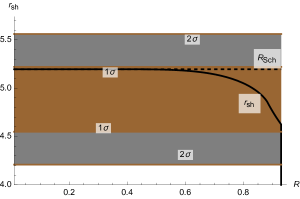
Figure 1: Constraints of black hole with de Sitter core from the Event Horizon Telescope horizon-scale image of Sagıttarius A* at $1\sigma$Vagnozzi et al. (2023), after averaging the Keck and VLTI mass-to-distance ratio priors for the same with $M_{0}=1$, and varying $R$ .

Afterwards, we plot the Fig. 2 that the radius of the black hole’s shadow ($r_{sh}$) is computed for varying values of $\beta$. The shadow radius of the black hole with a Hagedorn fluid first decreases as the value of $\beta$ increases, then shadow radius increases as shown in 2. Moreover Fig. 2 displays the upper limits of $\beta$ based on EHT observational results for Sgr A*. The $68\%$ confidence level (C.L.) Vagnozzi et al. (2023) indicates that the upper limit for $\beta$ is $1.8$.

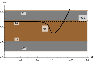
Figure 2: Constraints of black hole with Hagedorn fluid from the Event Horizon Telescope horizon-scale image of Sagıttarius A* at $1\sigma$Vagnozzi et al. (2023), after averaging the Keck and VLTI mass-to-distance ratio priors for the same with $M_{0}=1$, and varying $\beta$ .

V Formation of regular black hole and naked singularities

As we have found out in previous sections that solutions (15) with equation of state $P=k(r)\rho$ (with $k(r)=A+Br$) and (35) with Hagedorn fluid are alike under some conditions. Here, we study the gravitational collapse model with equation of state (14) of the spacetime in the Edington-Finkelstein coordinates $\{v,r,\theta,\varphi\}$:

$$ds^{2}=-\left(1-\frac{2M(v,r)}{r}\right)dv^{2}+2dvdr+r^{2}d\Omega^{2},$$ (47)

here, $M(v,r)$ is the mass function and $v$ advanced Eddington time. The spacetime (47) is supported by combination of two energy-momentum tensors of type-I and II describing null dust and null fluid respectively. This energy-momentum tensor can be written as

$$T^{tot}_{\mu\nu}=T^{ND}_{\mu\nu}+T^{NS}_{\mu\nu},$$ (48)

where $T^{ND}_{\mu\nu}$ is the energy-momentum tensor of null dust

$$T^{(ND)}_{\mu\nu}=\mu(v,r)l_{\mu}l_{\nu},$$ (49)

and $T^{NS}_{\mu\nu}$ represents null fluid

$$T^{(NS)}_{\mu\nu}=(\rho+P)(l_{\mu}n_{\nu}+l_{\nu}n_{\mu})+Pg_{\mu\nu},$$ (50)

where $l^{\mu}$ and $n^{\mu}$ are two null vectors with properties

$$l_{\mu}l^{\mu}=n_{\mu}n^{\mu}=0,~{}~{}n_{\mu}l^{\mu}=-1,$$ (51)

and have the form

$$l_{\mu} = \delta^{0}_{\mu},$$

$$n_{\mu} = \frac{1}{2}\left(1-\frac{2M}{r}\right)\delta^{0}_{\mu}-\delta^{1}_{\mu}.$$ (52)

$\mu$ is the energy density of the null dust and $\rho$ and $P$ are energy density and pressure of the null fluid respectively. They have the form

$$\mu(v,r) = \frac{2\dot{M}(v)}{r^{2}},$$

$$\rho(v,r) = \frac{2M^{\prime}(v,r)}{r^{2}},$$

$$P(v,r) = -\frac{M^{\prime\prime}(v,r)}{r}.$$ (53)

The Einstein field equations with equation of state (14) lead to the mass function of the form

$$M(r,v)=M_{0}(v)-\frac{w_{0}(v)}{2}\left(Rr^{2}+R^{2}r+\frac{R^{3}}{2}\right)e^{-\frac{2r}{R}}.$$ (54)

The physical quantities (V) are given by

$$\mu = \frac{2}{r^{2}}\left[\dot{M}_{0}(v)-\frac{\dot{w}_{0}(v)}{2}\left(Rr^{2}+R^{2}r+\frac{R^{3}}{2}\right)e^{-\frac{2r}{R}}\right],$$

$$\rho = 2w_{0}(v)e^{-\frac{2r}{R}},$$

$$P = 2w_{0}(v)\left(\frac{r}{R}-1\right)e^{-\frac{2r}{R}}.$$ (55)

V.1 Naked singularity formation

First, we consider the case when we have singularity formation, i.e. the condition

$$w_{0}(v)=\frac{4M_{0}(v)}{R^{3}},$$ (56)

is not held. The naked singularity might be the result of the gravitational collapse if the following conditions are fulfiling

• The time of the singularity formation is less than the time of the apparent horizon formation;

• there exists the family of non-spacelike, future-directed geodesics which terminate in the central singularity in the past.

The central singularity forms at $r=0$ at time $v=0$. In order to prove the existence of a family of non-spacelike, future-directed geodesics which terminate at the central singularity in the past, we consider the radial null geodesic which has the form

$$\frac{dv}{dr}=\frac{2}{1-\frac{2M_{0}}{r}+\frac{w_{0}}{r}\left(r^{2}R+rR^{2}+\frac{R^{3}}{2}\right)e^{-\frac{2r}{R}}}.$$ (57)

This geodesic terminates in the central singularity in the past if $\lim\limits_{v\rightarrow 0,r\rightarrow 0}\frac{dv}{dr}$ is finite and positive. Let us denote

$$\lim\limits_{v\rightarrow 0,r\rightarrow 0}\frac{v}{r}=X_{0}.$$ (58)

At the time of singularity formation, i.e. at $v=0$ the condition $M(0,0)=0$ must be held Mkenyeleye et al. (2014). In particular, this condition leads to

$$M_{0}(0)=w_{0}(0)=0.$$ (59)

If this condition is not held but we still have $M(0,0)=0$ then it means that $w_{0}=\frac{4M_{0}}{R^{3}}$, i.e. regular black hole formation. This case we will consider in next subsection.

Thus, one can write

$$M_{0}(v) \sim M_{00}v+\mathcal{O}(v^{2}),$$

$$w_{0}(v) \sim w_{00}v+\mathcal{O}(v^{2}),$$

$$M_{00} \equiv \dot{M}_{0}(0),$$

$$w_{00} \equiv \dot{w}_{0}(0).$$ (60)

Substituting (V.1) into (57) and taking into account the definition (58), we arrive at following algebraic equation

$$\xi X_{0}^{2} - X_{0}+2=0,$$

$$\xi \equiv 2M_{00}-\frac{1}{2}w_{00}R^{3}>0.$$ (61)

The last inequality follows from weak energy condition which states that $\mu>0$ (V). If eqrefeq:naked admits positive root, then the result of the gravitational collapse might be naked singularity. Solving this quadratic equation one obtains:

$$X_{0}^{\pm} = \frac{1}{2\xi}\left(1\pm\sqrt{1-8\xi}\right).$$ (62)

One can see that if $\xi\leq\frac{1}{8}$ then the result of the gravitational collapse might be naked singularity. Note, that in Vaidya spacetime, naked singularity forms if $M_{00}\leq\frac{1}{16}$. However, in our model $M_{00}$ can be greater than $\frac{1}{16}$, i.e. one has the following restriction

$$\xi\leq\frac{1}{8}\rightarrow M_{00}\leq\frac{1}{16}+\frac{w_{00}R^{3}}{2}.$$ (63)

V.2 Regular black hole formation

Now we consider the regular black hole formation. In this case

$$w_{0}(v)=\frac{4M_{0}(v)}{R^{3}}.$$ (64)

A black hole has a regular center if scalar invariants are regular in the limit $r\to 0$. Kretschmann scalar at the centre has the following form

$$K=\frac{32}{3}w_{0}^{2}(v)=\frac{512M_{0}(v)^{2}}{3R^{6}}.$$ (65)

One should note that the energy flux $\mu$ is equal to zero at the centre of a black hole because the condition (64) assumes $\dot{M}(v,0)=0$. From observational point of view, it is important to obtain information from the region with de Sitter core. To achieve this goal one should fulfil the following condition

• the apparent horizon should absent at $v=0$;

• there should be a family of non-spacelike, future-directed geodesics which goes from the centre of a star.

The absence of the apparent horizon at $v\rightarrow 0$assumes that $\lim\limits_{v\rightarrow 0}M(v,r)=0$. This property imposes the following condition on functions $M_{0}(v)$ and $w_{0}(v)$, i.e.

$$M_{0}(0)=0,~{}~{}w_{0}(0)=0.$$ (66)

Now, we should prove that at $v\rightarrow 0$ there is a radial null geodesic which future-directed. The radial null geodesic equation has the form

$$\frac{dv}{dr}=\frac{2}{1-\frac{2M(v,r)}{r}}.$$ (67)

Now, if we take a limit

$$\lim\limits_{v\rightarrow 0,r\rightarrow 0}\frac{dv}{dr}\equiv X_{0}=2,$$ (68)

i.e. this geodesic exists and is future directed. Thus, in this model, under some physical conditions, the de Sitter core can be observed by a distant observer. Here, we should point out the following property of obtained solution, i.e. singularity-regularity oscillation. Let us consider the function

$$N(v)\equiv w_{0}(v)-\frac{4M_{0}(v)}{R^{3}}.$$ (69)

If $N(v)\equiv 0$ then one has regular black hole. However, if $N(v)=0$ only at some points $v_{1},v_{2},v_{3}\cdots v_{n}$ then one has the following black hole: at the time $v=0$ the regular black hole formes, then in the interval $v\in(0,v_{1})$ there is a singularity. However, at the time $v=v_{1}$ the singularity disappears and we again have regular center, then in the interval $v\in(v_{1},v_{2})$ one has singularity and ETC. As an example let us consider the following choice of functions $M_{0}$ and $w_{0}$

$$M_{0}(v) = \mu v,~{}~{}\mu>0,$$

$$w_{0}(v) = \nu v^{2},~{}~{}\nu>0.$$ (70)

In this case, the function $N(v)$ is equal to zero in two points $v_{1}=0$ and $v_{2}=\frac{4\mu}{\nu R^{3}}$. Thus, at the time $v=v_{1}$ we have a regular black hole formation, then in the interval $v\in(v_{1},v_{2})$ we have singularity formation. However, at $v=v_{2}$ one again has regular center and at $v>v_{2}$ one has singular black hole formation.

VI Conclusion

In this paper, we have considered three new solutions of Einstein field equations (15), (35) and (54) describing a black hole. The first model (15) describes a simple model of a black hole with changing equation of state $P=k(r)\rho$. This solution can describe both and singular and regular black holes depending on parameters $M_{0}$ and $w_{0}$. The second model describes a black hole with Hagedorn fluid which is suitable equation of state for late stage of black hole formation. In general, this solution is hard to express in elementary functions. However, we considered a particular case (35) and found out that this solution is similar to the solution (15) and can describe a regular black hole as well as singular one. Then we study shadow cast of the new black hole solutions. The constraints on the black hole shadow radius ($R_{sh}$) for different theoretical models are derived from the Event Horizon Telescope (EHT) observations of Sagittarius A* (Sgr A*), as summarized below:

• Black Hole with De Sitter Core:
  
  - In Fig. 1, the shadow radius $r_{sh}$ is computed for varying values of $R$. The analysis indicates that $r_{sh}$ decreases as $R$ increases.
  
  - The EHT observational results for Sgr A* impose upper limits on $R$. At a $68\%$ confidence level (C.L.) Vagnozzi et al. (2023), the upper limit for $R$ is determined to be $0.9$, following the averaging of Keck and VLTI mass-to-distance ratio priors.

• Black Hole with Hagedorn Fluid:
  
  - As depicted in Fig. 2, the shadow radius $r_{sh}$ is calculated for varying values of $\beta$. Initially, $r_{sh}$ decreases with increasing $\beta$, but it begins to increase for higher values of $\beta$.
  
  - Based on the EHT observations for Sgr A*, the upper limits on $\beta$ are established. At a $68\%$ confidence level (C.L.) Vagnozzi et al. (2023), the upper limit for $\beta$ is found to be $1.8$, derived from the same observational data and priors used in the De Sitter core model.

These constraints provide significant insights into the properties of black holes with different core structures and surrounding matter distributions. The horizon-scale imaging data from the EHT, particularly for Sgr A*, play a crucial role in refining these models and enhancing our understanding of black hole physics.

The first two models describe static spherically-symetric black holes. However, real astrophysical objects gain and lose their masses during gravitational collapse, accretion or radiation. It means that the spacetime describing real astrophysical black holes should be dynamical one. On this reason, we consider dynamical version of the solution (15) and obtained the solution (54). Then we considered the process of gravitational collapse and found out that this process can lead to naked singularity formation. If we match functions $M_{0}(v)$ and $w_{0}(v)$ in such a way that a regular black hole forms then the de Sitter center can be observed by a distant observer. The key point of the solution (54) is that it can describe regular black hole then during the gravitational collapse it becomes singular and after some time it becomes regular again. The obtained solutions have an important astrophysical application:

• The obtained solutions can describe both and regular and singular black holes. It depends only on initial profile. As the result, by calculating a black hole shadow one can distinguish singular black hole from regular one through its shadow properties. It is important to note that we consider one model which will help us to find difference in shadow;

• investigating the motion of $S$ stars and other objects close to a black hole we can find out if the central object singular or regular black hole.

It is also very interesting to investigate the thermodynamical properties of obtained solutions. Especially, we should find out what happens at the time $v=v_{null}$ and if we have something special in two regimes when weak energy condition is valid and violated. Shadow properties of dynamical process of formation and evaporation of singular black hole is also important to better understand the nature of a black holes. For this purpose, one should elaborate the method of analytical calculation of a shadow of a dynamical black hole which is currently apsent. Although the first steps in this direction has been made in the paper Vertogradov and Övgün (2024b). The solution (54) has unusual behavior of the Kretschmann scalar, i.e. during the evolution it can be both and finite and infinite in the centre of a black hole. The process of a singularity formation is understandable because there are a lot of regular black hole solutions supported by non-linear electrodynamics and during neutralization the centre of a black hole becomes singular. However, the opposite process is unatural, i.e. we have the singularity formation then during the evolution it becomes regular. We have not countered this phenomenon before in literature. It should be carefuly investigated in order to give physical explanation of this process or to reject it according to some physically-relevant reasons. This problem we leave for our future research.