Evaluating and Utilizing Surrogate Outcomes in Covariate-Adjusted Response-Adaptive Designs

Abstract

This manuscript explores the intersection of surrogate outcomes and adaptive designs in statistical research. While surrogate outcomes have long been studied for their potential to substitute long-term primary outcomes, current surrogate evaluation methods do not directly account for the potential benefits of using surrogate outcomes to adapt randomization probabilities in adaptive randomized trials that aim to learn and respond to treatment effect heterogeneity. In this context, surrogate outcomes can benefit participants in the trial directly (i.e. improve expected outcome of newly-enrolled study participants) by allowing for more rapid adaptation of randomization probabilities, particularly when surrogates enable earlier detection of heterogeneous treatment effects and/or indicate the optimal (individualized) treatment with stronger signals. Our study introduces a novel approach for surrogate evaluation that quantifies both of these benefits in the context of sequential adaptive experiment designs. We also propose a new Covariate-Adjusted Response-Adaptive (CARA) design that incorporates an Online Superlearner to assess and adaptively choose surrogate outcomes for updating treatment randomization probabilities. We introduce a Targeted Maximum Likelihood Estimation (TMLE) estimator that addresses data dependency challenges in adaptively collected data and achieves asymptotic normality under reasonable assumptions without relying on parametric model assumptions. The robust performance of our adaptive design with Online Superlearner is presented via simulations. Our framework not only contributes a method to more comprehensively quantifying the benefits of candidate surrogate outcomes and choosing between them, but also offers an easily generalizable tool for evaluating various adaptive designs and making inferences, providing insights into alternative choices of designs.

1 Introduction

1.1 Motivation

Surrogate outcomes are often considered as a substitute for the primary outcome when the primary outcome requires a long follow-up time or is expensive to measure. Their most significant application is in clinical trials. Potential advantages of using surrogates to replace primary outcomes include early detection of treatment effects, accelerated drug approvals, and reduced costs (Buyse et al., 2000). For example, vaccine-induced immune responses can be surrogate endpoints for HIV infection (Gilbert and Hudgens, 2008). Surrogate outcomes are also valuable in non-health sectors. For example, in digital experiments conducted by private sector companies, experimenters seek to identify useful surrogates to replace primary outcomes that take time to measure, thereby accelerating decisions on new product launches (Duan et al., 2021; Richardson et al., 2023).

While surrogate outcomes have long been studied for their potential to substitute for long-term primary outcomes in clinical trials, current surrogate evaluation methods do not directly account for the potential benefits of using surrogate outcomes to adapt randomization probabilities in randomized adaptive designs that aim to learn and respond to treatment effect heterogeneity. In contrast to traditional randomized controlled trials that assigns participants to treatment groups with fixed (and usually equal) probabilities throughout the study, adaptive randomization designs introduces a dynamic approach, modifying the allocation of participants to treatment groups based on data collected as the experiment progresses. This flexibility allows adaptive randomization to serve several specific objectives, such as maximizing the statistical precision for estimating the parameter of interest or increasing the likelihood that participants receive the more effective treatments as indicated by real-time evidence.

Among various types of adaptive experimental designs, Response-Adaptive Randomization (RAR) and Covariate-Adjusted Response-Adaptive (CARA) designs are useful to achieve the second objective Rosenberger and Lachin (2015); Robertson et al. (2023). In RAR, the randomization of treatment allocation depends on the treatments and outcomes (responses) from previous participants; treatment randomization probabilities in RAR are adapted to favor a single treatment that shows greater promise based on accumulated data of previous participants. CARA designs further enhance adaptivity by incorporating baseline covariates as a factor to adjust treatment randomization probabilities in response to estimated heterogeneous treatment effects (Rosenberger et al., 2001; Rosenberger and Sverdlov, 2008; Atkinson et al., 2011). In CARA, to achieve the goal of more particpants receiving the treatment that is best for them, treatment randomization probabilities can be adjusted for new patients based on their covariates, favoring the individualized optimal treatments learned from previous data. This approach is useful in contexts where treatment effects and optimal treatments vary among different subgroups without a single treatment that is uniformly optimal for all participants.

While RAR and CARA designs offer the compelling advantage of increasing benefits for participants within a study through their adaptive nature, they encounter limitations when dealing with outcomes that require long follow-up times. In such scenarios, the delay in observable responses hinders randomization probabilities from being adapted promptly, potentially diminishing the designs’ real-time optimization procedure.

In this context, surrogate outcomes, which measured earlier than the primary outcome, have the potential to enhance the benefit of adaptive randomization for participants within the experiment directly (i.e. improve the expected outcome of newly-enrolled participants) by allowing for more rapid adaptation of randomization probabilities, particularly when surrogates, if any, allow for earlier detection of heterogeneous treatment effects. However, the challenge becomes more complex when there are multiple candidate surrogates, raising the question of which surrogate is most useful to replace the primary outcome to facilitate the CARA procedure.

Many statistical methods to evaluate surrogate outcomes in traditional clinical trials have not yet been optimized for this sequential decision-making problem posed by CARA experiments. Specifically, in these designs, the timing of the availability of the surrogate outcome plays a critical role, including potential tradeoffs between the immediacy of early surrogates and their sensitivity and accuracy in indicating optimal treatments. For example, early proxies of primary outcomes can serve as candidate surrogate outcomes. One possible trade-off arises when these early proxies are partially effective (i.e. imperfect surrogates) in identifying the best personalized treatments. Their use as a surrogate allows for an earlier adaptation of randomization probabilities towards more effective treatments for many participants, compared to waiting for the final outcome. However, using these imperfect early proxies can also skew randomization probabilities towards sub-optimal treatments for some participants. Conversely, waiting for final outcomes before adapting randomization probabilties risks delaying benefits for early particpants and skewing randomization probabiltiies towards suboptiomal treatments for early particpants due to insufficient data. The sensitivity of a surrogate to treatment effect heterogeneity is a crucial driver of these trade-offs. A surrogate that is better able to accurately detect heterogeneous treatment effect will lead to a higher probability of participants receiving more effective treatments, compared to one that exhibits less sensitivity.

In short, adaptation of randomization probabilities based on a surrogate, as opposed to the final outcome, has the potential to either help or harm participants in a study. The optimal decision of whether or not to adapt randomization based on a surrogate or to wait for the final outcome, and if using a surrogate, which surrogate to use, is determined by complex trade-offs between the timeliness of the surrogate (i.e., the ability of a candidate surrogate to provide more information earlier about which treatments work best for which patients) and the quality of information a surrogate provides (i.e., the ability of a surrogate to accurately and sensitively reflect optimal treatment assignments conditional on covariates). Navigating these tradeoffs requires both novel approaches for quantifying the benefit of candidate surrogates, and novel designs and estimators that make possible online evaluation of these benefits and dynamic surrogate selection in response during the course of a study.

While existing methods for surrogate evaluation predominantly assess statistical or causal relationships between surrogate and primary outcomes, few methods directly quantify these benefits of surrogates beyond predicitivity. Furthermore, current surrogate evaluation approaches typically evaluate surrogates using data from completed randomized controlled trials or observational studies, making it difficult to capture the aforementioned nuanced and time-sensitive benefits of using surrogates in such static retrospective analyses.

In this work, we are motivated to adopt an adaptive design perspective to evaluate surrogates and propose an approach that evaluates surrogates within the context of Covariate-Adjusted Response-Adaptive (CARA) designs, thereby offering a more comprehensive understanding of surrogates’ utilities. Our target parameter is defined based on a counterfactual adaptive design in which each participant’s treatment assignment probability would be optimized to maximize the expected reward indicated by a candidate surrogate outcome, conditional on previous participants’ data collected before current participant enrollment. Our target is to estimate the expected mean of the primary outcome under this hypothetical adaptive design. This target parameter embodies the previously mentioned considerations by accounting for both the quality of information a surrogate outcome provides and its timing in driving decision-making to maximize benefits for trial participants.

We utilize this criterion to provide a new CARA design with an online selection tool (which we call “Online Superlearner”) that evaluates all potential surrogate outcomes in real-time and selects a surrogate to be used to update treatment randomization probabilities for new participants.

To estimate this target parameter, we propose a Targeted Maximum Likelihood Estimator (TMLE) (Van der Laan et al., 2011; Van der Laan and Rose, 2018; van der Laan, 2008), addressing the technical challenge of making statistical inference on our target parameter based on non-i.i.d data collected from adaptive experiments. We obtain a consistent and asymptotically normal TMLE estimator by leveraging the martingale central limit theorem and maximal inequalities for martingale processes, without relying on parametric assumptions. Our TMLE framework (including the analysis of its asymptotic normality) is generally applicable to help answer other causal questions that would be of interest in regular randomized controlled trials, such as Average Treatment Effect, and the expected reward under optimal treatment rules (regimes) (Murphy, 2003; Luedtke and Van Der Laan, 2016) for maximizing surrogate outcomes and the final outcome.

More broadly, our framework for implementing adaptive designs with Online Superlearner is easily generalizable to evaluate and select from a variety of adaptive designs distinguished by various characteristics, not limited to different surrogates. As experimenters may only determine one specific adaptive design at each time point, our evaluation framework offers a counterfactual reasoning approach to offer insights into how the reward might differ under alternative design choices, and provides a way to choose one from various candidate designs for real-time sequential decision-making processes.

1.2 Related Work

Surrogates outcomes. Surrogate outcomes have been an active field of statistical research. Many statistical methods have been proposed to evaluate surrogate outcomes, including but not limited to Prentice’s criteria (Prentice, 1989), proportion of treatment effect explained (PTE) (Freedman et al., 1992; Lin et al., 1997), direct and indirect causal effects frameworks (Robins and Greenland, 1992; Joffe and Greene, 2009), principal stratification frameworks (Frangakis and Rubin, 2002; Gilbert and Hudgens, 2008) and meta-analysis frameworks (Daniels and Hughes, 1997; Buyse et al., 2000). One can find a thorough review and discussion of surrogate evaluation methods in VanderWeele (2013), Weir and Taylor (2022) and Elliott (2023). However, existing methods are genrally focused on their ability of surrogates to accurately reflect treatment effects on the primary outcome, and do not directly quantify other key metrics of a surrogate’s value in the context of adaptive trial designs, such as speed and accuracy with which the surrogate can identify heterogeneous treatment effects, and the implications for the primary outcome of the patient’s enrolled in the trial. Our target parameter integrates these considerations to evaluate the utility of surrogate outcomes in CARA designs, offering a more comprehensive and realistic assessment of surrogates’ potentials and providing a robust tool for surrogate selection.

Adaptive Experimental Designs. Adaptive designs are another active research area in causal inference and experimental designs. In clinical trials, adaptive design methods have become very popular due to their flexibility and efficiency (Chow and Chang, 2008). Adaptive designs allow for modifications to eligiblity criteria, randomization probabilities, and other key design features based on the sequentially accrued data during the ongoing experiment. Such adaptivity can also be applied to online A/B testing in digital experiments. Among various kinds of adaptive designs, the Response-Adaptive Randomization (RAR) design presents a procedure that allows the treatment randomization scheme to be changed based on the treatment and response of subjects enrolled previously, with the aim of achieving different targeted experimental objectives, ranging fron gaining efficiency in learning treatment effects to bringing more welfare to subjects in experiments (i.e. minimizing regret) (Hu and Rosenberger, 2006; Robertson et al., 2023). One can further implement a Covariate-Adjusted Response-Adaptive (CARA) design, which allows the adaptation of treatment randomization probabilities to depend on baseline covariates of existing subjects (Rosenberger et al., 2001; Rosenberger and Sverdlov, 2008; Atkinson et al., 2011). Tracing its origins to the seminal work of Thompson (1933); Robbins (1952), the RAR and CARA experimental designs with the objective of bringing the welfare of the study participants, are intrinsically linked to a substantial body of research on Multi-Arm Bandits (MAB) and their derivative, Contextual Bandits (CB) (see Bubeck et al. (2012); Lattimore and Szepesvári (2020)). A significant portion of this research is dedicated to exploring the efficiency of various algorithms in minimizing regret (see survey in Simchi-Levi and Wang (2023)).

Using surrogate outcomes to facilitate RAR / CARA design. The use of surrogate outcomes is also discussed in some literature on RAR designs, as they can be quickly observed when the primary outcome is delayed (Robertson et al., 2023). Tamura et al. (1994) uses a short-term response to conduct adaptive randomization to treat out-patients with depressive disorder. Huang et al. (2009) uses a Bayes mixture distribution to model the relationship between surrogates and primary outcomes to facilitate RAR procedure. McDonald et al. (2023) utilizes a pre-trained Bayesian reward model to run bandits without delay. Yang et al. (2023) considers using an external dataset to construct a surrogate outcome to impute the missing primary outcome to run contextual bandit algorithms. While these approaches allow for earlier deployment of CARA procedure before observing primary outcome data, either relying on prior knowledge, external dataset or generalization assumptions, our framework equips researchers with a tool to dynamically re-evaluate multiple candidate surrogates in their comprehensive utility in CARA design and refine their surrogate choice within the ongoing sequential decision-making environment.

Inference after adaptive experiments. Our estimation method is related to the challenge of drawing statistical inference based on data collected from adaptive experiments, which is an important research question considered in the adaptive design literature. For example, Zhang et al. (2007); Zhu (2015) established asymptotic results for making statistical inferences from data generated by CARA designs under correctly specified models. Following van der Laan (2008), Chambaz and van der Laan (2014) proposed a CARA design targeting an optimal design for estimating the risk difference and log-relative risk, and provides statistical inference robust to model mis-specification with Targeted Maximum Likelihood Estimation (TMLE) (Van Der Laan and Rubin, 2006; Van der Laan et al., 2011; Van der Laan and Rose, 2018) methodology. Chambaz et al. (2017) established a CARA design targeted for estimating the mean outcome of the optimal treatment rule, and proved a central limit theorem which enables the construction of confidence intervals without relying on parametric model assumptions. Recently, several works used a stabilized doubly robust estimator, following an approach originally proposed by (Luedtke and Van Der Laan, 2016) to provide inference for the mean outcome under a possibly non-unique optimal treatment strategy, to make valid inference to evaluate treatment effects or the mean outcome under a target treatment rule in non-contextual setting (Hadad et al., 2021) and contextual setting (Bibaut et al., 2021; Zhan et al., 2021).

While the focus of these methodologies has been to infer the counterfactual mean outcome under a static treatment rule, either as preordained by the user or as an data-adaptive optimal treatment rule learned from the data, we propose a distinct target parameter that is able to reflect the timeliness of a surrogate outcome in facilitating the sequential decision-making process with CARA procedures. Specifically, we propose as target parameter the counterfactual mean outcome across a sequence of stochastic treatment rules, which are optimized to maximize a surrogate outcome, conditional on the finite-dimensional summary measure of historical data before making a treatment decision for each participant. This general approach draws on related work on causal inference for time-series data (van der Laan and Malenica, 2018; Malenica et al., 2021, 2024), where the target estimand is defined as an average of a series of time-specific treatment rules conditional on the summary measure of the historical data before each time point.

The rest of the manuscript is organized as follows. In Section 2, we present the statistical setup of our CARA designs and introduce the target parameters for surrogate evaluation. Next, we describe the estimation procedure using TMLE and detail how our adaptive design is implemented with the Online Superlearner that evaluates and selects surrogates to faciliate CARA procedure. Section 3 introduces the sampling schemes we employed to update treatment randomization probabilities in our design. In Section 4, we explore the asymptotic properties of our TMLE estimator. Simulation results are presented in Section 5, followed by extensions, discussions and concluding remarks in Section 6.

2 Data, Model, and Statistical Setup of CARA Experiments

We consider a sequential CARA experiment for a longitudinal data structure. Suppose we have binary treatment $A$ from the set $\mathcal{A}=\{0,1\}$. We use $W\in\mathcal{W}$ to denote the baseline covariates of subjects. Let $Y_{K}$ denote the final outcome we are interested in, where $K$ denotes the follow-up time required to observe $Y_{K}$ after assigning a treatment to each subject. We suppose that $Y_{K}$ falls within the range of $0$ to $1$ and that higher values indicate better outcomes. Similarly, we consider $K-1$ shorter-term surrogate outcomes, denoted by $Y_{k}$; the follow-up times required to observe these outcomes range from $k=1$ to $k=K-1$, respectively.

Let $T$ represent the total duration of the adaptive experiment. At each time point $t$, the experimenter reviews historical data related to a surrogate outcome $Y_{k}$. Using the data available before time $t$, the experimenter estimates the Conditional Average Treatment Effect (CATE) for the surrogate outcome $Y_{k}$. The CATE for a user with covariate $w$ is defined $E[Y_{k}|A=1,W=w]-E[Y_{k}|A=0,W=w]$. Based on the estimated CATE function of $Y_{k}$, and the baseline covariates of new subjects enrolled at time $t$, the experimenter generates a treatment randomization function $\tilde{g}_{k,t}:\mathcal{A}\times\mathcal{W}\to[0,1]$ that maps treatment levels and covariate values to a treatment probability in the range $[0,1]$. This function is used to adjust treatment randomization probabilities for all subjects newly enrolled at time $t$. More details about how to estimate CATE functions and how to adapt treatment randomization probabilities based on this CATE estimate will be introduced in Section 3.1.

In light of the aforementioned trade-offs in utilizing different surrogates in adaptive designs, we introduce a novel adaptive design that incorporates evaluation and selection of the most effective surrogate online (i.e., using an approach that continually updates as new data are accrued), without replying on prior knowledge. This design incorporates a surrogate evaluation procedure assessing each surrogate’s utility through a target estimand. This estimand quantifies the expected average reward in the final outcome $Y_{K}$ for each subject, assuming they were treated in a hypothetical (or coutnerfactual) adaptive design that was responsive to a surrogate outcome at the time of their enrollment. We use Targeted Maximum Likelihood Estimation (TMLE) to estimate the target estimands and identify the surrogate with the largest lower confidence bound of the TMLE estimate. This surrogate is then utilized to adjust treatment randomization probabilities for newly enrolled subjects. This approach enhances the design’s adaptivity and effectiveness by selecting surrogates that are more likely to yield benefits for subjects within the experiment.

In this section, we first outline notations for data and model. Then we define a general target parameter, which evaluates each candidate surrogate within a counterfactual adaptive design.

2.1 Statistical Setup

We begin by introducing the notation for the observed data and the causal model on the observed data generating process. Let $E(t)$ subjects at each time point $t$, and define $N(t)=\sum_{t^{\prime}=1}^{t}E(t^{\prime})$ as the cumulative number of participants enrolled up to time $t$. For each participant $i$, we observe $O_{i}=(t_{i},W_{i},A_{i},Y_{i,1},\cdots,Y_{i,K})$ where $t_{i}$ is entry time; $W_{i}$ and $A_{i}$ are the baseline covariates and treatment, observed at time $t_{i}$; at time $t_{i}+k$, we observe $Y_{i,1},...,Y_{i,K-1}$ are $K-1$ surrogate outcomes with follow-up time from $1$ to $K-1$, respectively. At time $t_{i}+K$, we observe $Y_{i,K}$, the final outcome of interest of the $i$-th participant. In order to emphasize the chronological time that each node is observed, we define $\tilde{W}_{i}(t_{i})=W_{i},\tilde{A}_{i}(t_{i})=A_{i}$, and $\tilde{Y}_{i}(t_{i}+k)=Y_{i,k}$ for $k=1,\cdots,K$. We use the two sets of notations interchangeably. We then denote the historical data from time $1$ to $t-1$ by $\bar{O}(t-1)=\{{\tilde{W}_{i}(t^{\prime}):i\in[N(t-1)],t^{\prime}\leq t-1}\}\bigcup\{\tilde{A}_{i}(t^{\prime}):i\in[N(t-1)],t^{\prime}\leq t-1\}\bigcup\{\tilde{Y}_{i}(t^{\prime}):i\in[N(t-1)],t^{\prime}\leq t-1\}$.

As time moves from $t-1$ to $t$, we will observe more nodes from two groups of subjects: $R_{1}(t)=\{i:t-K\leq t_{i}\leq t-1\}$ and $R_{2}(t)=\{i:t_{i}=t\}$. $R_{1}(t)$ are all previously enrolled participants who haven’t reached their endpoint before time $t$; $R_{2}(t)$ are all subjects who enter the experiment beginning at time $t$. We define that at each time $t$, we first observe outcomes $Y_{i,t-t_{i}}$ for all $i\in R_{1}(t)$, subsequently observe $W_{i}$, and then assign $A_{i}$ for each $i\in R_{2}(t)$.

We use $\overline{\mathcal{H}}(t)=\bar{O}(t-1)\bigcup\{\tilde{Y}_{i}(t),i\in R_{1}(t)\}$ to denote the historical data before the observation of $\{(W_{i},A_{i}),i\in R_{2}(t)\}$, the covariate and treatment nodes for subjects in $R_{2}(t)$. We define $\tilde{g}_{t}:\mathcal{A}\times\mathcal{W}\to[0,1]$ as a time $t$-specific function that presents the conditional distributions of $A$ given $W$. Let $\mathcal{G}_{t}$ denote a set of conditional distributions of $A$ given $W$ that includes $\tilde{g}_{t}$. We note that $\tilde{g}_{t}$ is itself a mapping from $\overline{\mathcal{H}}(t)$ to $\mathcal{G}_{t}$. In an adaptive experiment, $\tilde{g}_{t}$ is defined based on historical data $\overline{\mathcal{H}}(t)$, and subsequently used to assign treatment randomization probabilities to every new unit $i\in R_{2}(t)$ based on their baseline covariates $W_{i}$.

To formalize this for individual participants within the experiment, we define $\mathcal{H}(i):=(\overline{\mathcal{H}}(t_{i}),W_{i})$ to denote the unit $i$-specific historical data before treatment $A_{i}$. We focus on an $i$-specific stochastic rule that depends on $\mathcal{H}(i)$ through a fixed dimensional summary measure $C_{i}:=f_{C}(\mathcal{H}(i))\in\mathcal{C}$, where $f_{C}$ is a fixed function that maps the historical data $\mathcal{H}(i)$ into a fixed-dimensional real-valued space. In practice, we require that $C_{i}$ always includes the baseline covariates $W_{i}$. Given the summary measure $C_{i}$ before $A_{i}$, we define $g_{i}(\cdot|C_{i}):\mathcal{A}\to[0,1]$ as the function of assigning treatment randomization probability for any $a\in\mathcal{A}=\{0,1\}$.

Let $q_{W}$ denote the marginal density of $W$, and $q_{Y_{k}}$ denote the conditional density of outcome $Y_{k}$ given $W,A,Y_{1},\cdots,Y_{k-1}$ ($k=1,\cdots,K$). We can represent the likelihood of data $\bar{O}(t)$ by

$$p\left(\bar{O}(t)\right) =\prod_{i=1}^{N(t)}q_{W}(w_{i})g_{i}(a_{i}|C_{i})\times\prod_{k=1}^{\min(K,t-t_{i})}q_{Y_{k}}(y_{i,k}|w_{i},a_{i},y_{i,1},\cdots,y_{i,k-1})$$

We define $\bar{Q}_{k}(A,W)=E(Y_{k}|A,W)$ to be the conditional mean for $k=1,\cdots,K$, and define $\theta=(g,q_{w},\bar{Q}_{1},\cdots,\bar{Q}_{K})\in\mathcal{G}\times\mathcal{Q}_{W}\times\bar{\mathcal{Q}}_{1}\times\cdots\times\bar{\mathcal{Q}}_{K}$. $\bar{Q}_{1},\cdots,\bar{Q}_{K}$ are common functions across all units. Conditional on the realized summary $C_{i}$ of every unit $i$, the statistical model of distributions of $O_{i}$ is $\mathcal{M}(C_{i})=\{P_{\theta,C_{i}}:\theta\}$.

Let $\bar{O}_{i}(t)$ denote the cumulative data $O_{i}$ observed up to time $t$ for the $i$-th participant. We can rewrite the conditional likelihood of $\bar{O}_{i}(t)$ up to time $t$, given the observed summary measure $C_{i}$ as follows:

$$p_{\theta,C_{i}}(o_{i}) =q_{W}(w_{i})g_{i}(a_{i}|C_{i})\prod_{k=1}^{t-t_{i}}q_{Y_{k}}(y_{i,k}|w_{i},a_{i},y_{i,1},\cdots,y_{i,k-1}).$$

We specify a Structural Causal Model (SCM) (Pearl et al., 2000) for variables of new unit $i$ enrolled at time $t_{i}$ by

$$W_{i} =f_{W}(U_{W_{i}}),$$

$$\mathcal{H}(i) =(\overline{\mathcal{H}}(t),W_{i}),$$

$$C_{i} =f_{C}(\mathcal{H}(i)),$$

$$A_{i} =f_{A}(C_{i},U_{A_{i}}),$$

$$Y_{i,k} =f_{Y_{k}}(W_{i},A_{i},Y_{i,1},\cdots,Y_{i,k-1},U_{Y_{i,k}}),k=1,\cdots,K,$$

where $U_{i}=(U_{W,i},U_{A,i},U_{Y_{i,1}},\cdots,U_{Y_{i,K}})$ are unmeasured and independent exogenous variables and follow the same distribution across all units. We use $g_{0,i}$ to denote the actual stochastic rule to assign treatments for unit $i$, and $\mathbf{g}_{0,1:n_{t}}=(g_{0,1},\cdots,g_{0,n_{t}})$ denote the actual adaptive design that we assign treatments and collect data.

2.2 A General Target Parameter to Evaluate Mean Outcome under a Counterfactual CARA Design

We first propose a general target parameter of interest under a modified SCM under any counterfactual adaptive design. We start by defining a vector of summary measures $\bar{C}^{*}(n):=(C_{1}^{*},\cdots,C_{n}^{*})$, which are generated sequentially in a counterfactual adaptive design denoted by $\mathbf{g}_{*,1:n}(\bar{C}^{*}(n)):=(g_{*,i}(\cdot|C_{i}^{*}))_{i=1,\cdots,n}$, where each $g_{*,i}(\cdot|C_{i}^{*})$ is a stochastic treatment rule $\mathcal{A}\to[0,1]$, depending on $C_{i}^{*}$. The generations of $\bar{C}^{*}(n)$ and $\mathbf{g}_{*,1:n}(\bar{C}^{*}(n))$ are illustrated in the following modified SCM:

$$W_{i} =f_{W}(U_{W}),$$

$$\mathcal{H}^{*}(i) =(\overline{\mathcal{H}}^{*}(t_{i}),W_{i}),$$

$$C_{i}^{*} =f_{C}(\mathcal{H}^{*}(i)),$$

$$A_{i}^{*} \sim g_{*,i}(\cdot|C_{i}^{*}),$$

$$Y_{i,k}^{*} =f_{Y_{k}}(W_{i},A_{i}^{*},Y_{i,1}^{*},\cdots,Y_{i,k-1}^{*},U_{Y_{k}}),k=1,\cdots,K,$$

in which $f_{A}$ nodes are replaced by stochastic rules $g_{*,i}(\cdot|C_{i}^{*})$. We note that each element $C_{i}^{*}$ influences the subsequent treatment rule $g_{*,i}(\cdot|C_{i}^{*})$, thus impacting the subsequent $A_{i}$, $Y_{i,k}$, and $C_{i+1}$. This model highlights the iterative and cumulative impact had we intervened with a series of counterfactual stochastic treatment rules.

An ideal target parameter of interest is the counterfactual expectation of $Y_{K}^{*}$ under the counterfactual adaptive design $\mathbf{g}_{*,1:n}(\bar{C}^{*}(n))$ generated by that modified SCM. While it is theoretically feasible to identify this target parameter by using the $g$-computation formula Robins (1986, 1987), it results in a complex statistical estimand, for which any estimation procedure would be computationally intensive in the nested data structure where any small change in early nodes could have a cumulative impact on follow-up nodes.

Instead, we modify our target parameter by following the causal inference framework for single time-series data, as introduced in van der Laan and Malenica (2018) and Malenica et al. (2021). We set up another SCM that is modified as follows:

$$W_{i} =f_{W}(U_{W}),$$

$$\mathcal{H}(i) =(\overline{\mathcal{H}}(t_{i}),W_{i}),$$

$$C_{i}^{*} =f_{C}(\mathcal{H}^{*}(i)),$$

$$A_{i}^{*} \sim g_{*,i}(\cdot|C_{i}),$$

$$Y_{i,k}^{*} =f_{Y_{k}}(W_{i},A_{i}^{*},Y_{i,1}^{*},\cdots,Y_{i,k-1}^{*},U_{Y_{k}}),k=1,\cdots,K,$$

where our $g_{*,i}$ is defined by the observed summary measure $C_{i}$ for every unit $i$. Under this simplified SCM with less modification, we propose the following data-adaptive parameter conditional on $\bar{C}(n):=(C_{1},\cdots,C_{n})$:

$$\Psi_{\mathbf{g}_{*,1:n}\left(\bar{C}(n)\right)}=\frac{1}{n}\sum_{i=1}^{n}E_{g_{*,i}\left(\cdot|C_{i}\right)}\left[Y_{i,K}^{*}\right],$$

which targets the counterfactual final outcome of all units had they been treated, at their entry time, by different stochastic rules given the summary measures observed from the experiment.

Remark 1. While the cumulative impact over $\bar{C}^{*}(n)$ and $\mathbf{g}_{*,1:n}(\bar{C}^{*}(n))$ may appear unpredictable, such concerns are mitigated under a well-designed CARA framework, which makes our target parameter $\Psi_{\mathbf{g}_{*,1:n}\left(\bar{C}(n)\right)}$ a viable alternative estimand to circumvent the identification and estimation complexities by with the $g$-formula. Specifically, in Section 3, we discuss the CARA framework where each $C_{i}$ only depends on CATE functions estimated from previous data and the surrogate selected by Online Superlearner. In this setting, any change in early context primarily affects the proportion of treatment and control observed in subsequent stages, without altering the true CATE functions to be estimated. By applying a doubly-robust estimator for CATE functions using pseudo-outcomes (Van der Laan, 2006; Luedtke and van der Laan, 2016), we expect such impact will be mild on future contexts and the choice of surrogate in the Online Superlearner in our setup, thanks to the stationarity in the outcome models and our knowledge of true treatment probabilities in the adaptive design. We refer readers to Section 9.1 in Malenica et al. (2021) for a detailed discussion about the statistical and computational advantages of context-specific parameters compared to marginal target parameters. While comparing these two types of parameters could itself be an interesting direction for future research, for the remainder of this paper, we focus on evaluating counterfactual adaptive designs by using $\Psi_{\mathbf{g}_{*,1:n}\left(\bar{C}(n)\right)}$ as our target parameter, which can be robustly estimated under sequential adaptive designs with a lower computational burden.

3 Evaluating and Utilizing Surrogates within CARA design

In this section, we first introduce how we design a CARA procedure to adapt treatment randomization probabilities. Then we define our target parameter, which evaluates each candidate surrogate within a counterfactual adaptive design that utilizes the surrogate to adapt treatment randomization probabilities. Following this, we will demonstrate how to use the TMLE of the target parameter to evaluate surrogates. Finally we will introduce a new CARA design that incorporates an Online Superlearner to identify and utilize the most useful surrogate.

3.1 A Class of CARA Designs that Use Surrogates to Adapt Treatment Randomization Probabilities

We focus on a class of CARA designs that utilize a candidate surrogate as a response to adapt treatment randomization probabilities, following an extension of the strategy proposed by Chambaz et al. (2017).

We define a treatment randomization function $h_{m}:[-1,1]\times\mathbb{R}^{+}\to[0,1]$ as follows:

$$h_{m}(x,b)=m\mathds{1}(x\leq-b)+(1-m)\mathds{1}(x\geq b)+\left(\frac{1/2-m}{2b^{3}}x^{3}+\frac{1/2-m}{2b/3}x+\frac{1}{2}\right)\mathds{1}\left(-b\leq x\leq b\right),$$

where $m\in[0,0.5]$ is a user-specified constant such that $m<|h_{m}|<1-m$. Let $B_{0,k}:\mathcal{W}\to[-2,2]$ denote the true CATE function $E[Y_{k}\mid 1,W]-E[Y_{k}\mid 0,W]$ of an outcome $Y_{k}$ ($k=1,\cdots,K$). Let $B_{n,k}(w_{i})$ denote an estimate of CATE of $Y_{k}$ based on $w_{i}$, the baseline covariates of unit $i$. We use $\tau_{n,k}(w_{i})$ to denote the estimated standard error of CATE of unit $i$. Both estimates are based on $\mathcal{H}(i)$, the historical data observed before unit $i$ is enrolled. We employ a doubly-robust estimator to estimate CATE functions using pseudo-outcomes (Van der Laan, 2006; Luedtke and van der Laan, 2016) and applying Highly Adaptive Lasso van der Laan (2015, 2017); Benkeser and van der Laan (2016); van der Laan (2023) to obtain $B_{n,k}$ and $\tau_{n,k}$ (see Appendix B). Users are flexible to define their own methods to estimate them.

Then we use $h_{m}$ to map $C_{i}$ to a treatment randomization probability between 0 and 1. We define a three-dimensional, $k$-specific summary measure $C_{i,k}=\left(w_{i},B_{n,k}(w_{i}),\tau_{n,k}(w_{i})\right)$ for every $k\in[K]$, the index for surrogate $Y_{k}$. Taking the union of $C_{i,k}$ across $k\in[K]$, we define $C_{i}:=(C_{i,k})_{k=1}^{K}$ as the complete summary measure before treatment decision for unit $i$. Recall that $g^{*}_{k,i}(a\mid C_{i})$ describes the treatment randomization probability tailored for optimizing a surrogate outcome $Y_{k}$, based on summary measure $C_{i}$. $g^{*}_{k,i}$ is generated by the following equation:

$$g^{*}_{k,i}(a|C_{i})=\begin{cases}h_{m}\left(B_{n,k}(w_{i}),z_{1-\alpha/2}\cdot\tau_{n,k}(w_{i})\right)&a=1,\\ 1-h_{m}\left(B_{n,k}(w_{i}),z_{1-\alpha/2}\cdot\tau_{n,k}(w_{i})\right)&a=0,\end{cases}$$

where $z_{1-\alpha/2}$ is the $1-\alpha/2$-th quantile of standard normal distribution ($\alpha=0.05$).

Our strategy balances exploration and exploitation based on the CATE functions learned from the data. Intuitively, $g^{*}_{k,i}(a|C_{i})$ depends on the confidence interval of the estimated CATE of $Y_{k}$ for participant $i$: $B_{n,k,i}(w_{i})\pm z_{1-\alpha/2}\cdot\tau_{n,k,i}(w_{i})$. The more deviated the confidence interval is from zero, the more likely it is to assign unit $i$ to an optimal individual treatment. Note that $m$ is the lower bound of the randomization probability of assigning a sub-optimal treatment, and $1-m$ is the upper bound of the probability to assign optimal treatment. If the confidence interval excludes zero, we assign the better treatment with probability $1-m$. If no $Y_{k}$ has been observed before the enrollment of unit $i$, we set $g^{*}_{k,i}=0.5$.

3.2 Target Parameter to Evaluate Surrogates under Counterfactual CARA Designs

As a specification of the general target parameter under a hypothetical adaptive design (as introduced in Section 2.2), we consider $K$ candidate adaptive designs $\mathbf{g}^{*}_{k,1:n_{t}}$ ($k=1,\cdots,K$) for all units enrolled from time $1$ to $t-K$ with complete follow-up, using $n_{t}=N(t-K)$ to denote the total number of units till time $t-K$. In the $k$-th design $\mathbf{g}^{*}_{k,1:n_{t}}$, the stochastic rule $g^{*}_{k,i}$ is generated by the estimated conditional average treatment effect on the surrogate outcome $Y_{k}$ using nodes $W$, $A$ and $Y_{k}$ observed from historical data $\mathcal{H}(i)$. We define the following target parameter for each surrogate $Y_{k}$:

$$\Psi_{t,k}:=\Psi_{t,\mathbf{g}^{*}_{k,1:n_{t}}}=\frac{1}{n_{t}}\sum_{i=1}^{n_{t}}E_{g^{*}_{k,i}}\left[Y_{i,K}^{*}\right].$$

We refer to this parameter of “the utility of a candidate surrogate” in the CARA design. Our target parameter corresponds to the expected final outcome $Y_{K}$ of all $n_{t}$ units had they been treated, at their entry time, by a stochastic rule tailored to optimize the mean outcome of an early surrogate $Y_{k}$. We will use this target parameter to evaluate the utility of different surrogate outcomes in the CARA design, and utilize this to choose the surrogate to be used for updating the treatment allocation strategy used for the next time point in the ongoing adaptive design.

Let $Q_{0}:=(\bar{Q}_{0,K},Q_{0,W})\in\bar{\mathcal{Q}}_{K}\times\mathcal{Q}_{W}$, where $Q_{0,W}$ is the true distribution of $W$, and $\bar{Q}_{0,K}$ is the true conditional mean function of the final outcome $Y_{K}$ given $A$ and $W$. We can identify our causal estimand (i.e., the utlity of a candidate surrogate) by the observed data under the following assumptions. Since the investigators are designing the adaptive experiments, they can ensure that the causal identification assumptions hold by carefully specifying their designs.

Assumption 1 (Sequential Randomization).

For any $k\in[K]$ and every subject $i\in\{1,\cdots,n_{t}\}$, we have $Y_{i,k}(a)\perp\!\!\!\perp A_{i}\mathrel{|}C_{i}$.

Assumption 2 (Positivity).

For any subject $i$, $g_{0,i}(a_{i}|C_{i})>0$ for every $a_{i}\in\mathcal{A}$.

Theorem 1 (Identification).

With assumptions 1 and 2, one can identify $\Psi_{t,k}(Q_{0})$ from the observed data by

$$\Psi_{t,k}(Q_{0})=\Psi_{t,\mathbf{g}^{*}_{k,1:n_{t}}}(Q_{0})=\frac{1}{n_{t}}\sum_{i=1}^{n_{t}}E_{g^{*}_{k,i},Q_{0}}\left[Y_{i,K}^{*}\right]=\frac{1}{n_{t}}\sum_{i=1}^{n_{t}}\sum_{a=0}^{1}\bar{Q}_{0,K}(a,w_{i})g^{*}_{k,i}(a|C_{i})\\ .$$

Remark 2. Our target parameter evaluates the utility of surrogates by their early availability, as well as their predictability and sensitivity in indicating effective treatments, defined in the following sense. We define a trajectory of stochastic treatment rules $\tilde{g}^{*}_{k,1:t}:=(\tilde{g}^{*}_{k,1},\cdots,\tilde{g}^{*}_{k,t})$, with each rule $\tilde{g}^{*}_{k,t^{\prime}}$ generating personalized stochastic rules $g^{*}_{k,i}$ for each participant $i$ enrolled at time $t^{\prime}$. The rule $g^{*}_{k,i}$ is specifically tailored to maximize the surrogate outcome $Y_{k}$ based on their baseline covariates. We note that at each time point $t^{\prime}$, $\tilde{g}^{*}_{k,t^{\prime}}$ only depends on historical data $\overline{\mathcal{H}}(t^{\prime})$. Therefore, $\tilde{g}^{*}_{k,t^{\prime}}$ can not deviate from a static design with equal randomization probabilities during the initial $k$ time points, as observation of $Y_{k}$ is not yet available. Once $Y_{k}$ is available at $t^{\prime}=k+1$, $\tilde{g}^{*}_{k,t^{\prime}}$ starts moving towards its optimal treatment rule $d_{0,k}(W):=I\left(\bar{Q}_{0,k}(1,W)-\bar{Q}_{0,k}(0,W)>0\right)$ over time. If $d_{0,k}$ closely aligns with the true optimal rule for the primary outcome $d_{0,K}$, then the surrogate $Y_{k}$ demonstrates the advantage of its early availability in informing which treatment is better in the context of sequential decision making, compared to later outcomes. As is shown in Section 3.1, the progression of $\tilde{g}^{*}_{k,t^{\prime}}$ from a static design with equal randomization probabilities towards the optimal treatment rule $d_{0,k}$ depends on the magnitude of treatment superiority (as measured by the point estimate of CATE) and its uncertainty (as reflected by estimated standard error of CATE). Therefore, if a surrogate $Y_{k}$ exhibits good alignment with the primary outcome in terms of optimal treatment rule and presents a strong signal of individualized optimal treatment over other surrogates, this surrogate will be preferred and given a higher $\Psi_{t,k}$. Of course, even if a surrogate demonstrates early availability and sensitivity, it will be assigned a lower $\Psi_{t,k}$ value if it fails to predict optimal personalized treatments. This is because the ultimate evaluation of a surrogate’s performance is based on the primary outcome, underscoring the critical role of predictability in evaluating surrogate outcomes in adaptive designs. In summary, our proposed causal parameter quantifies the utility of a candidate surrogate and thus provides a summary measure that incorporates these trade-offs.

3.3 Targeted Maximum Likelihood Estimation

We propose using a Targeted Maximum Likelihood Estimator (TMLE) to estimate $\Psi_{t,k}$. Let $\bar{Q}_{n,K,t}(A,W)$ be an initial estimate of $\bar{Q}_{0,K}(A,W)$ based on the historical data $\bar{H}(t)$ observed up till time $t$. One can employ the Super Learner (Van der Laan et al., 2007) or Highly Adaptive Lasso (Benkeser and van der Laan, 2016; van der Laan et al., 2022) to obtain an initial estimator $\bar{Q}_{n,K,t}$ of the conditional mean function $\bar{Q}_{0,K}$. Then we apply a TMLE procedure to update $\bar{Q}_{n,K,t}$ by fitting the following logistic model

$$\mathop{\mathrm{logit}}\bar{Q}_{n,K,t,\epsilon}\left(A,W\right)=\mathop{\mathrm{logit}}\bar{Q}_{n,K,t}\left(A,W\right)+\epsilon$$

with weights $\frac{g^{*}_{k,i}(a_{i}|C_{i})}{g_{0,i}(a_{i}|C_{i})}$ (Van Der Laan and Rubin, 2006; Van der Laan et al., 2011; Malenica et al., 2024). The estimate of $\epsilon$ is denoted by $\hat{\epsilon}_{t}$, and an updated estimator of the conditional mean function, $\bar{Q}_{n,K,t}^{*}:=\bar{Q}_{n,K,t,\hat{\epsilon}_{t}}$, is obtained, which solves the following estimating equation:

$$\frac{1}{n_{t}}\sum_{i=1}^{n_{t}}\frac{g^{*}_{k,i}(a_{i}|C_{i})}{g_{0,i}(a_{i}|C_{i})}\left(Y_{i,K}-\bar{Q}_{n,K,t}^{*}(a_{i},w_{i})\right)=0.$$

The TMLE estimate for $\Psi_{t,k}$ is thus given by

$$\hat{\Psi}_{t,k}=\frac{1}{n_{t}}\sum_{i=1}^{n_{t}}\sum_{a=0}^{1}\bar{Q}_{n,K,t}^{*}(a,w_{i})g^{*}_{k,i}(a|C_{i}).$$

We estimate the standard error of $\hat{\Psi}_{t,k}$ by $\sqrt{\frac{1}{n_{t}}\hat{\sigma}^{2}_{t,k}}$, where

$$\hat{\sigma}^{2}_{t,k}=\frac{1}{n_{t}}\sum_{i=1}^{n_{t}}\left[\frac{g^{*}_{k,i}(a_{i}|C_{i})}{g_{0,i}(a_{i}|C_{i})}\left(Y_{i,K}-\bar{Q}_{n,K,t}^{*}(a_{i},w_{i})\right)\right]^{2}.$$

We also provide the following confidence interval for $\hat{\Psi}_{t,k}$:

$$\left[\hat{\Psi}_{t,k}-z_{1-\alpha/2}\sqrt{\frac{1}{n_{t}}\hat{\sigma}^{2}_{t,k}},\hat{\Psi}_{t,k}+z_{1-\alpha/2}\sqrt{\frac{1}{n_{t}}\hat{\sigma}^{2}_{t,k}}\right],$$

where $z_{1-\alpha/2}$ is the $1-\alpha/2$-th quantile of standard normal distribution ($\alpha=0.05$). This method is widely applicable for estimating the target parameter $\Psi_{\mathbf{g}_{*,1:n}\left(\bar{C}(n)\right)}$ under a general counterfactual adaptive design $\mathbf{g}_{*,1:n}\left(\bar{C}(n)\right)$, as introduced in Section 2.2.

3.4 Online Superlearner that Selects Surrogate Outcomes in CARA Experiments

As we progress to a new time point $t$, we have up to $K$ candidate stochastic rules $g^{*}_{1,i},\cdots,g^{*}_{k,i}$ for assigning treatment randomization probabilities for a new participant $i$ enrolled at $t$. For each $k$, the stochastic rule $g^{*}_{k,i}$ is generated based on historical data, specifically tailored to optimize the mean outcome of $Y_{k}$. We next propose the use of an Online Superlearner to select the most useful surrogate at time $t$ (denoted as $Y_{k^{*}_{t}}$), which is used to guide subsequent treatment randomization decisions; importantly, this approach allows surrogate selection to depend on information about a surrogate’s utility accrued during the study, and allows this surrogate selected to evolve over the course of the study. This process begins by estimating $\hat{\Psi}_{t,k}$ for each $k\in[K]$ and obtaining confidence intervals for these estimates. The surrogate $Y_{k^{*}_{t}}$ is then determined by identifying $k^{*}_{t}$, which is defined as:

$$k^{*}_{t}=\mathop{\mathrm{argmax}}_{k\in[K]}\hat{\Psi}_{t,k}-z_{1-\alpha/2}\sqrt{\frac{1}{n_{t}}\hat{\sigma}^{2}_{t,k}},$$

where $k^{*}_{t}$ corresponds to the surrogate with the highest lower confidence interval bound among all $\hat{\Psi}_{t,k}$ for $k=1,\cdots,K$. Finally, for all units $i$ enrolled at time $t$, we assign treatment randomization probabilities using $g^{*}_{k_{t}^{*},i}$.

Remark 3. We note that in adaptive designs in which randomization probabilities are adapted in response to an outcome $Y_{k}$, all participants would be randomly assigned to different treatment groups with equal probability prior to the first observation of surrogate $Y_{k}$ at $t=k+1$ (Section 3.1). Similarly, in our adaptive design with the Online Superlearner, every treatment decision before $t=K+1$ is randomly made by flipping a fair coin. This is because the surrogate evaluation procedure is only activated after the primary outcome $Y_{K}$ has been observed for the initially enrolled subset of participants. While we will propose in Section 6 a modified adaptive design that is able to initiate surrogate evaluation and the adapt treatment randomization probabilities at an earlier stage, the adaptive designs investigated within this section represent the most conservative approaches ensuring that every adaptation, without exception, is activated only subsequent to the observation of related outcomes within the ongoing experimental environment. Such conservativeness helps maintain reliability in adapting treatment randomization probabilities and evaluating surrogates.

While the optimal choice of a surrogate is not known a priori in practice, our Online Superlearner will identify the most useful surrogate for maximizing reward as more data accumulates. It will then adjust the actual treatment randomization probabilities towards the optimal treatment rule associated with that surrogate. Consequently, our design will converge to a design that improves the efficiency in estimating the mean outcome under the optimal treatment rule of that most useful surrogate.

3.5 Statistical Inference at the End of CARA Experiments

When the experiment ends at time $T$, one can follow the same methodology outlined in Section 3.3 to estimate $\Psi_{T,k}$. Furthermore, we note that the non-i.i.d. data collected from our adaptive experiments also allow us to identify and estimate (with rigorous inference) other causal questions typically answered in randomized controlled trials. These questions include evaluating the average treatment effect and the expected reward under optimal treatment rules for both surrogate outcomes and the final outcome. For these target parameters, a doubly-robust TMLE estimator is feasible, specifically designed to handle the challenges of data dependency while ensuring asymptotic normality. The methodology for constructing TMLEs for these parameters mirrors the approach of making statistical inference for our target parameter $\Psi_{T,k}$ and the other parameters shown in van der Laan (2008); Chambaz et al. (2017); Bibaut et al. (2021); Malenica et al. (2021, 2024).

For example, one might be interested in other questions and have other target parameters from the data collected from adaptive designs. For example, given an estimate $d^{*}_{n,k,T}$ of $d_{0,k}(W)$, the true optimal treatment rule of $Y_{k}$. One can establish the following modified SCM :

$$W =f_{W}(U_{W})$$

$$A^{*} \sim d^{*}_{n,k,T}(W)$$

$$Y_{k}^{*} =f_{Y_{k}}(W,A^{*},Y_{1}^{*},\cdots,Y_{k-1}^{*},U_{Y_{k}}),k=1,\cdots,K$$

had everyone is treated by $d^{*}_{n,k,T}$. Under this modified SCM, one can propose a target parameter $\psi_{d^{*}_{n,k,T}}=E_{d^{*}_{n,k,T}}[Y_{K}]$, the mean final outcome $Y_{K}$ under an estimated optimal treatment rule for a surrogate $Y_{k}$. To estimate $\psi_{d^{*}_{n,k,T}}$, one can first obtain an initial estimator $\bar{Q}_{n,K,t}(A,W)$ and apply the TMLE procedure to solve the following estimating equation:

$$\frac{1}{n_{T}}\sum_{i=1}^{n_{T}}\frac{d^{*}_{n,k,T}(a_{i}|C_{i})}{g_{0,i}(a_{i}|C_{i})}\left(Y_{i,K}-\bar{Q}_{n,K,T}^{*}(a_{i},w_{i})\right)=0.$$

Then we can plug $\bar{Q}_{n,K,T}^{*}(A,W)$ and the empirical distribution of $Q_{W}$ into $\psi_{T,k}$ to get an TMLE

$$\hat{\psi}_{d^{*}_{n,k,T}}=\frac{1}{n_{T}}\sum_{i=1}^{n_{T}}\bar{Q}_{n,K,t}^{*}(d^{*}_{n,k,T}(w_{i}),w_{i}).$$

We can estimate its standard error by $\sqrt{\frac{1}{n_{T}}\hat{\sigma}^{2}_{d^{*}_{n,k,T}}}$, where

$$\hat{\sigma}^{2}_{d^{*}_{n,k,T}}=\frac{1}{n_{T}}\sum_{i=1}^{n_{T}}\left[\frac{d^{*}_{n,k,T}(a_{i}|C_{i})}{g_{0,i}(a_{i}|C_{i})}\left(Y_{i,K}-\bar{Q}_{n,K,T}^{*}(a_{i},w_{i})\right)+\bar{Q}_{n,K,T}^{*}(d^{*}_{n,k,T}(w_{i}),w_{i})-\hat{\psi}_{d^{*}_{n,k,T}}\right]^{2}.$$

However, since $d^{*}_{n,k,T}$ is learned from the data itself, the regular TMLE estimate is biased upward for the mean outcome under the rule. We recommend using cross-validated TMLE (CV-TMLE) (Zheng and Van Der Laan, 2010; van der Laan and Luedtke, 2015; Montoya et al., 2021), which uses internal sample splitting to avoid finite sample bias.

We note that $\psi_{d^{*}_{n,k,T}}=E_{d^{*}_{n,k,T}}[Y_{K}]$ can be an interesting supplemental target parameter to evaluate a surrogate, as it reflects the mean primary outcome under the surrogate-based optimal treatment rule. This type of approach was also introduced in Hsu et al. (2015) and Yang et al. (2023). However, similar to most existing surrogacy evaluation methods and in contrast to the surrogate utility parameter we proposed, this measure does not evaluate the timeliness and sensitivity of surrogates in detecting effective treatments.

4 Theoretical Analysis of TMLE

In this section, we show consistency and asymptotically normality property of TMLE $\hat{\Psi}_{t,k}$ by decomposing its difference from the truth $\Psi_{t,k}$ into a sum of martingale difference sequence and a martingale process and analyzing them by Martingale Central Limit Theorem and equicontinuity conditions.

For any $\bar{Q}_{K}\in\bar{\mathcal{Q}}_{K}$ we define

$$D_{k}(\bar{Q}_{K})\left(O_{i},C_{i}\right)=\frac{g^{*}_{k,i}\left(A_{i}|C_{i}\right)}{g_{0,i}\left(A_{i}|C_{i}\right)}\left(Y_{i,K}-\bar{Q}_{K}\left(A_{i},W_{i}\right)\right),$$

where $C_{i}$ is a summary measure, including baseline covariates $W_{i}$. theoremrepThmDecomposition For any $\bar{Q}_{n,K,t}^{*}\in\bar{\mathcal{Q}}_{K}$ and $\bar{Q}_{0,K}\in\bar{\mathcal{Q}}_{0,K}$, the difference between $\hat{\Psi}_{t,k}$ and $\Psi_{t,k}$ can be decomposed as

$$\hat{\Psi}_{t,k}-\Psi_{t,k}=M_{1,n_{t}}(\bar{Q}_{0,K})+M_{2,n_{t}}(\bar{Q}_{n,K,t}^{*},\bar{Q}_{0,K}),$$

where

$$M_{1,n_{t}}\left(\bar{Q}_{0,K}\right) =\frac{1}{n_{t}}\sum_{i=1}^{n_{t}}\left[D_{k}\left(\bar{Q}_{0,K}\right)\left(O_{i},C_{i}\right)-E\left[D_{k}\left(\bar{Q}_{0,K}\right)\left(O_{i},C_{i}\right)|\mathcal{H}(i)\right]\right],$$

$$M_{2,n_{t}}\left(\bar{Q}_{n,K,t}^{*},\bar{Q}_{0,K}\right) =\frac{1}{n_{t}}\sum_{i=1}^{n_{t}}\Biggl{[}\biggl{[}D_{k}\left(\bar{Q}_{n,K,t}^{*}\right)\left(O_{i},C_{i}\right)-E\left[D_{k}\left(\bar{Q}_{n,K,t}^{*}\right)\left(O_{i},C_{i}\right)|\mathcal{H}(i)\right]\biggr{]}$$

$$-\biggl{[}D_{k}\left(\bar{Q}_{0,K}\right)\left(O_{i},C_{i}\right)-E\left[D_{k}\left(\bar{Q}_{0,K}\right)\left(O_{i},C_{i}\right)|\mathcal{H}(i)\right]\biggr{]}\Biggr{]}.$$

4.1 Analysis of the first term

We first analyze the asymptotic normality of the first term $\sqrt{n_{t}}M_{1,n_{t}}(\bar{Q}_{0,K})$, which is a sum of martingale difference sequence. This is true because both $g^{*}_{k,i}(a_{i}|C_{i})$ and $g_{0,i}(a_{i}|C_{i})$ are known and dependent on historical data $H(i)$ only through $C_{i}$, while $\bar{Q}_{K}(a_{i},w_{i})$ also depends on $C_{i}$ as we require $w_{i}$ is a component of $C_{i}$. Therefore, one can apply a martingale central limit theorem for $\sqrt{n_{t}}M_{1,n_{t}}(\bar{Q}_{0,K})$. Assumptions 3 and 4 constitute a set of sufficient conditions for the asymptotic normality of (a) $D_{k}(\bar{Q}_{0,K})$ remains bounded, and (b) the average of conditional variances of $D_{k}(\bar{Q}_{0,K})$ stablizes.

Assumption 3 (Strong positivity).

For every $i$, there exists $\zeta>0$ such that $g_{0,i}>\zeta$ and $g^{*}_{k,i}>\zeta$.

Assumption 4 (Stabilization of the average of conditional variances).

There exists $\sigma^{2}_{t,k}\in\mathbb{R}^{+}$ such that

$$\frac{1}{n_{t}}\sum_{i=1}^{n_{t}}Var\left[D_{k}(\bar{Q}_{0,K})(O_{i},C_{i})\mid\mathcal{H}(i)\right]\overset{p}{\to}\sigma^{2}_{t,k}$$

Theorem 2 (Asymptotic normality of the first term).

Suppose that assumptions 3 and 4 hold, then

$$\sqrt{n_{t}}M_{1,n_{t}}\left(\bar{Q}_{0,K}\right)\overset{d}{\to}N(0,\sigma^{2}_{t,k}),$$

Proof.

The result is a direct consequence of various versions of martingale central limit theorems (e.g. theorem 2 in Brown (1971)). ∎

4.2 Analysis of the second term

Now we suppress the notation $t$ by denoting the sample size $n_{t}$ by $N$, the estimated conditional mean of final outcome $\bar{Q}_{n,K,t}^{*}$ by $\bar{Q}_{N,K}^{*}$ and the equicontinuity term $M_{2,n_{t}}$ by $M_{2,N}$. Suppose $\bar{\mathcal{Q}}_{0,K}\in\bar{\mathcal{Q}}_{K}$ and $\bar{\mathcal{Q}}_{N,K}^{*}\in\bar{\mathcal{Q}}_{K}$. To construct an asymptotically normal estimator, we need the negligibility of the second term $M_{2,N}(\bar{Q}_{N,K}^{*},\bar{Q}_{0,K})$, i.e.

$$M_{2,N}(\bar{Q}_{N,K}^{*},\bar{Q}_{0,K})=o_{P}(N^{-\frac{1}{2}}).$$

Let $N_{\infty}({\epsilon},\bar{\mathcal{Q}}_{K})$ denote the $\epsilon$-covering number in supremum norm of $\bar{\mathcal{Q}}_{K}$. We define $J_{\infty}({\epsilon},\bar{\mathcal{Q}}_{K}):=\int_{0}^{\epsilon}\sqrt{\log\left(1+N_{\infty}({\epsilon},\bar{\mathcal{Q}}_{K})\right)}du$ as the $\epsilon$-entropy integral in supremum norm of $\bar{\mathcal{Q}}_{K}$.

assumptionrepAssmptReasonableCoveringIntegral $\bar{\mathcal{Q}}_{K}$ is a class of functions with finite sup-norm covering number $N_{\infty}({r},\bar{\mathcal{Q}}_{K})$.

assumptionrepAssmpSigmaNConvergence Define $\sigma_{N}\left(\bar{Q}_{K},\bar{Q}_{0,K}\right):=\sqrt{\frac{1}{N}\sum_{i=1}^{N}E_{P_{0}}\left[\phi\left(\frac{|D_{k}\left(\bar{Q}_{K}\right)(O_{i},C_{i})-D_{k}\left(\bar{Q}_{0,K}\right)(O_{i},C_{i})|}{Z}\right)\bigm{|}C_{i}\right]}$, where $\phi(x)=e^{x}-x-1$, $Z=\frac{16(1-\zeta)^{2}}{\zeta^{2}}$. Assume that $\sigma_{N}(\bar{Q}_{N,K}^{*},\bar{Q}_{0,K})=o_{P}(1).$

theoremrepThmEquicontinuity (Equicontinuity of the Martingale Process Term) Suppose Assumptions 3, 4.2, 4.2 hold. Then $M_{2,N}(\bar{Q}_{N,K}^{*},\bar{Q}_{0,K})=o_{P}(N^{-\frac{1}{2}})$. The proof depends on general results in Appendix C, which proves equicontinuity of martingale process in a general setup (see Theorem 5 and Corollary 5). We leave the proof of Theorem 4.2 for adaptive design to Appendix D.

Recent work of van der Laan (2023) introduces a class of $k$-th order smoothness functions with bounded sectional variation norm on up to their $k$-th-order derivatives and the higher order spline Highly Adaptive Lasso (HAL) estimator, which will be reviewed in Appendix A. The theoretical results in van der Laan (2023) imply that if $\bar{Q}_{0,K}$ is in that class of functions and $\bar{Q}_{N,K}$ is estimtated by higher order spline Highly Adaptive Lasso (HAL), we can prove the equicontinuity condition without relying on Assumption 4.2. More details about these results are discussed in Appendix C.

assumptionrepAssmpHigherOrderSpline $\bar{Q}_{0,K}$ and $\bar{Q}_{N,K}^{*}$ are from a class of functions that are represented by a $k$-th order ($k=1,2,\cdots$) smooth function whose $k$-th order derivatives are Càdlàg functions with bounded variation norm (van der Laan, 2023). corollaryrepCoroHighOrderSplineEquicontinuity Suppose Assumptions 3 and 4.2 hold. Then $M_{2,N}(\bar{Q}_{N,K}^{*},\bar{Q}_{0,K})=o_{P}(N^{-\frac{1}{2}})$. We leave the proof of Theorem 4.2 to Appendix D, which depends on the general result of Corollary 5 in Appendix C.

4.3 Asymptotic normality of the TMLE

Theorem 3 (Asymptotic normality of the TMLE).

Suppose assumptions 3, 4, 4.2 4.2 hold, or alternatively, assumptions 3, 4, 4.2 hold, then

$$\sqrt{n_{t}}(\hat{\Psi}_{t,k}-\Psi_{t,k})\overset{d}{\to}N(0,\sigma^{2}_{t,k}).$$

We estimate the standard error $\sigma^{2}_{t,k}$ by $\hat{\sigma}^{2}_{t,k}=\frac{1}{n_{t}}\sum_{i=1}^{n_{t}}\left\{\frac{g^{*}_{k,i}\left(A_{i}\mid C_{i}\right)}{g_{0,i}\left(A_{i}\mid C_{i}\right)}\left[Y_{i,K}-Q_{n,K,t}^{*}\left(A_{i},W_{i}\right)\right]\right\}^{2}$ (which converges in probability to $\sigma^{2}_{t,k}$), and provide a confidence interval

$$\left[\hat{\Psi}_{t,k}-z_{1-\alpha/2}\sqrt{\frac{1}{n_{t}}\hat{\sigma}^{2}_{t,k}},\hat{\Psi}_{t,k}+z_{1-\alpha/2}\sqrt{\frac{1}{n_{t}}\hat{\sigma}^{2}_{t,k}}\right].$$

The asymptotic normality of $\hat{\Psi}_{t,k}-\Psi_{t,k}$ is directly obtained from the asymptotic normality of the first term $\sqrt{n_{t}}M_{1,n_{t}}(\bar{Q}_{0,K})$ and the equicontinuity condition in the second term $M_{2,n_{t}}\left(\bar{Q}_{n,K,t}^{*},\bar{Q}_{0,K}\right)=o_{p}\left(n_{t}^{-\frac{1}{2}}\right)$.

5 Simulations

We have introduced a new adaptive design with an Online Superlearner that evaluates multiple surrogates online and, at each time point at which randomization is occuring, adaptively selects one of them to guide the assignment of treatment randomization probabilities for newly enrolled subjects, with the overall objective of maximizing reward (minimizing regret) for subjects enrolled in the trial. In this section, we present simulation studies aimed at evaluating the performance of this adaptive design with the Online Superlearner and comparing it to other designs, including a traditional fixed Randomized Controlled Trial (RCT) design and $K$ adaptive designs, each guided by an individual surrogate $Y_{k}$ ($k=1,\cdots,K-1$) or the final outcome $Y_{K}$.

In our simulation setup, we consider a binary treatment $A\in\{0,1\}$, a one-dimensional baseline covariate $W$, which follows a uniform distribution $U(-4,4)$, four surrogate outcomes $Y_{k}$ measured at follow-up times $k=1,2,3,4$, respectively, and a final outcome $Y_{5}$ measured at follow-up time 5. Each unit’s outcome $Y_{k}$ is generated by its conditional mean $E(Y_{k}|A,W)$ plus a random noise following the normal distribution $N(0,1)$. We estimate conditional mean functions using Super Learner (Van der Laan et al., 2007), which incorporates Random Forest (Breiman, 2001), XGBoost (Chen and Guestrin, 2016) and first-order Highly Adaptive Lasso (HAL) estimator (van der Laan, 2023). The CATE functions and their pointwise confidence intervals are estimated using the first-order HAL estimator. More details are provided in Appendix B.

We evaluate the performance of various designs in two scenarios. In Scenario 1, the conditional mean functions of $Y_{k}$ given $A$ and $W$ are $E(Y_{k}|A,W)=(2A-1)\times\left(0.5-\frac{1}{1+e^{-(3-k)W}}\right)$. The CATE function is shown in the left of Figure 1. In this scenario, the optimal treatment rule (based on the final outcome of interest) is more aligned with the optimal treatment rule defined in terms of later versus earlier surrogates. This implies that, despite requiring some time to measure and thus delaying adaptation in randomization probabilities, later surrogates are more useful in guiding treatment assignment probabilities so that more people are treated by the correct individualized optimal treatment that maximizes the reward measured by the final outcome.

In Scenario 2, the conditional mean functions of $Y_{k}$ are $E(Y_{k}|A,W)=(2A-1)\times\left(0.5-\frac{1}{1+e^{-\gamma_{k}W}}\right)$, where $\gamma_{1}=3$,$\gamma_{2}=2$,$\gamma_{3}=1$,$\gamma_{4}=0.5$ and $\gamma_{5}=0.25$. The CATE functions are shown in the right of Figure 1. In this scenario, all surrogate outcomes have the same optimal treatment rule as that of the final outcome. Notably, early surrogates demonstrate a larger absolute value in the conditional average treatment effect (CATE) compared to later surrogates. This suggests that early surrogates are more sensitive to different treatments, potentially making them superior indicators of the most beneficial treatment compared to the final outcome. In other words, in this scenario, earlier surrogates have the joint advantage of both timeliness and improved sensitvity for detecting treatment effect heterogeneity.

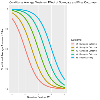
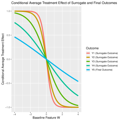
Figure 1: Conditional Average Treatment Effect (CATE) functions for Scenario 1 (left), in which later surrogates have higher utility and Scenario 2 (right) in which earlier surrogates have higher utility. Each curve represents the CATE function of a candidate surrogate, ranging from $Y_{1}$ to $Y_{5}$.

For each design, we run experiments for $T=50$ time points, enrolling 50 subjects at every time point. We compare three designs varying in their strategy to assign treatment randomization probability:

• simple sequential RCT, which randomly allocates two treatments with equal probability throughout the experiment;

• adaptive designs in response to an a priori fixed choice of either a surrogate outcome $Y_{k}$ ($k$ = 1, …, 4) or based on the final outcome $Y_{K}$ ($K=5$);

• adaptive design with Online Superlearner that selects an outcome from $Y_{1},\cdots,Y_{5}$ at each time point.

We set $m=0.1$ in $h_{m}$ to generate our stochastic rule in each adaptive design. Therefore, treatment allocation probabilities $g_{0,i}$ and $g^{*}_{k,i}$ are all bounded between 0.1 and 0.9.

We evaluate the performance of our adaptive design by assessing its ability to identify the oracle surrogate $Y_{k_{t}^{*}}$, which has the highest $\Psi_{t,k}$ at time $t$, and the regret associated with not assigning subjects to their optimal treatments.

5.1 Surrogate Evaluation Performance within the Online Superlearner

Our objective is to evaluate if our adaptive design with Online Superlearner can consistently identify the oracle surrogate, which we define as the candidate with the highest true $\Psi_{t,k}$ at time $t$ among all $Y_{k}$ (in other words, the surrogate that if used would result in the optimal expected outcomes for all persons in the trial). The oracle surrogate is the surrogate that results in the adaptive experiment updating treatment randomization probabilities towards true optimal individualized treatments such that benefit for participants is maximized.

Table 1 presents the average of true $\Psi_{t,k}$ values at times 11, 21, 31, 41, and 50 for Scenarios 1 and 2 across 500 Monte Carlo simulations. Additionally, $\Psi_{t,RCT}$, the expected outcome of $Y_{5}$ under a non-adaptive simple randomized controlled trial, is reported for both scenarios. The table highlights the expected reward for subjects enrolled up to time $t-K$, under the adaptive design defined by the oracle surrogate, denoted as $\Psi_{t,k_{t}^{*}}$, in bold at each respective time point $t$. Table 2 compares the probability of not assigning optimal personalized treatment within different designs.

In Scenario 1, the oracle surrogate with the highest $\Psi_{t,k_{t}^{*}}$ gradually shifts towards later surrogates as time elapses and more data from these surrogates become available to guide the adaptation of treatment randomization probabilities. Initially, surrogates $Y_{3}$ and $Y_{4}$ have the highest value at times 11 and 21, which are contributed by their early availability and moderate predictability in indicating personalized optimal treatments. While they show their utility by bringing more benefits in the short term, they do not consistently predict the correct optimal treatment for the primary outcome across all subgroups, leading them to be eventually outperformed by designs that utilize the true primary outcome $Y_{5}$ as additional follow-up time is accrued. This is expected, as the ultimate assessment of a surrogate’s effectiveness hinges on its ability to predict the optimal personalized treatment for primary outcome, highlighting the essential role of predictability in evaluating surrogate outcomes in adaptive designs.

In Scenario 2, surrogate $Y_{1}$ remains the most useful one throughout, due to its early availability, sensitivity and predictability in informing optimal individualized treatment for the long-term primary outcome. In constrast, later outcomes $Y_{4}$ and $Y_{5}$ have lower scores. This disparity can be attributed to the fact that while $Y_{4}$ and $Y_{5}$ may eventually contribute to identifying the optimal treatment as time goes infinitely, their utility is limited in the finite-time scenario. In such settings, designs that depend on later surrogates have a higher probability of assigning non-optimal treatment to participants due to their lower sensitivity and the fact that they provide less data for informed decision making. This limitation is demonstrated by the lower values in $\Psi_{t,4}$ and $\Psi_{t,5}$ compared to earlier surrogates.

Table 1: $\Psi_{t,k}$ in Scenario 1 and 2 ($t=11,21,31,41,50$).

(a) Scenario 1 $t$ $\Psi_{t,RCT}$ $\Psi_{t,1}$ $\Psi_{t,2}$ $\Psi_{t,3}$ $\Psi_{t,4}$ $\Psi_{t,5}$ 11 0 -0.013 0.054 0.078 0.065 0.033 21 0 -0.008 0.082 0.145 0.174 0.171 31 0 -0.004 0.088 0.160 0.201 0.206 41 0 -0.001 0.091 0.167 0.214 0.223 50 0 0 0.093 0.171 0.220 0.232

(b) Scenario 2 $t$ $\Psi_{t,RCT}$ $\Psi_{t,1}$ $\Psi_{t,2}$ $\Psi_{t,3}$ $\Psi_{t,4}$ $\Psi_{t,5}$ 11 0 0.072 0.057 0.039 0.018 0.004 21 0 0.086 0.080 0.072 0.059 0.037 31 0 0.089 0.085 0.080 0.071 0.050 41 0 0.091 0.088 0.084 0.077 0.058 50 0 0.092 0.090 0.086 0.080 0.063

Table 2: Probability (%) of not assigning optimal individualized treatments in Scenario 1 and 2 ($t=11,21,31,41,50$). $p^{\textit{non-opt}}_{t}:=\frac{1}{E(t)}\sum_{i:t_{i}=t}I\left(A_{i}\neq d_{0,K}(W_{i})\right)$, where $d_{0,K}(W):=I(\bar{Q}_{0,K}(1,W)-\bar{Q}_{0,K}(0,W)>0)$

(a) Scenario 1 $t$ $p^{\textit{non-opt}}_{t,SL}$ $p^{\textit{non-opt}}_{t,RCT}$ $p^{\textit{non-opt}}_{t,1}$ $p^{\textit{non-opt}}_{t,2}$ $p^{\textit{non-opt}}_{t,3}$ $p^{\textit{non-opt}}_{t,4}$ $p^{\textit{non-opt}}_{t,5}$ 11 27.9 49.8 51.0 40.3 29.8 20.6 17.1 21 20.6 50.3 50.3 39.9 30.4 20.2 15.0 31 17.4 49.8 50.5 39.7 29.5 20.1 13.8 41 16.4 49.8 50.3 40.0 29.9 19.9 13.4 50 15.7 50.5 49.8 39.6 30.5 20.1 13.6

(b) Scenario 2 $t$ $p^{\textit{non-opt}}_{t,SL}$ $p^{\textit{non-opt}}_{t,RCT}$ $p^{\textit{non-opt}}_{t,1}$ $p^{\textit{non-opt}}_{t,2}$ $p^{\textit{non-opt}}_{t,3}$ $p^{\textit{non-opt}}_{t,4}$ $p^{\textit{non-opt}}_{t,5}$ 11 15.2 50.5 14.6 14.8 16.3 20.5 30.4 21 13.7 50.1 13.0 13.4 14.1 16.8 23.4 31 12.8 49.5 12.1 12.8 13.7 15.7 20.9 41 12.4 50.2 12.0 12.3 12.9 15.5 18.9 50 13.1 49.2 11.9 12.1 13.1 14.7 18.4

Table 3 reports the coverage probability for the 95% confidence intervals corresponding to the true $\Psi_{t,RCT}$ and $\Psi_{t,k}$ at times 11, 21, 31, 41, and 50 in two scenarios across repeated Monte Carlo simulations. The results show that our confidence intervals reliably achieve the nominal coverage rate. These results underpin the reliability of subsequent analyses that calculate the selection frequency of the oracle surrogate within the Online Superlearner.

Table 3: Coverage probability (%) of confidence intervals for $\Psi_{t,k}$ in Scenario 1 and 2 ($t=11,21,31,41,50$).

(a) Scenario 1 $t$ $\Psi_{t,RCT}$ $\Psi_{t,1}$ $\Psi_{t,2}$ $\Psi_{t,3}$ $\Psi_{t,4}$ $\Psi_{t,5}$ 11 96.2 95.2 96.8 95.8 95.8 95.8 21 94.0 94.4 94.6 95.0 95.4 93.8 31 93.0 93.2 94.4 95.0 94.2 93.4 41 93.2 94.4 94.4 94.6 94.4 93.4 50 93.8 95.0 95.2 93.8 94.4 95.0

(b) Scenario 2 $t$ $\Psi_{t,RCT}$ $\Psi_{t,1}$ $\Psi_{t,2}$ $\Psi_{t,3}$ $\Psi_{t,4}$ $\Psi_{t,5}$ 11 94.6 94.4 94.0 93.8 95.4 95.6 21 95.4 95.6 96.2 95.2 95.6 95.2 31 94.6 95.6 95.4 94.6 94.8 95.8 41 95.6 96.6 95.8 96.0 95.4 97.0 50 94.8 96.6 96.0 96.8 95.8 96.0

Figure 2 tracks the frequency that each candidate adaptive design is selected by our proposed Online Superlearner at each time point $t$. Without prior knowledge of the relationships between various outcomes, the Online Superlearner is able to identify the oracle surrogate outcome for the adaptive design in each setting.

Recall that in Scenario 1, later surrogate outcomes serve as better proxies for the final outcome when determining optimal individualized treatments. The left part of Figure 2 shows that as the experiment progresses, with more observations of the final outcomes available, the Online Super Learner increasingly favors adaptive designs that correspond to later outcomes, ultimately selecting designs related to $Y_{4}$ and $Y_{5}$ with the highest frequency.

Conversely, in Scenario 2, the earliest surrogate outcome $Y_{1}$ emerges as the oracle surrogate, accurately pinpointing the optimal individualized treatment and presenting the highest $\Psi_{t,k}$ among its counterparts. As shown in the right part of Figure 2, the Online Superlearner, without a priori guidance, predominantly opts for adaptive designs that respond to early surrogates, selecting the design corresponding to $Y_{1}$ most frequently, followed by $Y_{2}$ and $Y_{3}$. In contrast, $Y_{4}$ and $Y_{5}$ are rarely chosen.

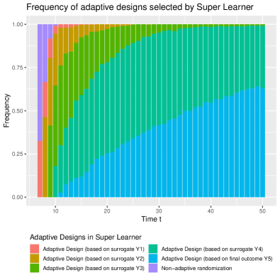
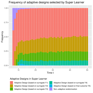
Figure 2: Frequency of candidate adaptive design selection by the Online Superlearner at each time point, differentiated by outcomes $Y_{k}$ ($k\in\{1,2,3,4,5\}$). The left panel shows Scenario 1 and the right panel Scenario 2. Each color presents a candidate surrogate outcome / final outcome from $Y_{1}$ to $Y_{5}$.The height of each bar indicates the frequency with which $\hat{\psi}_{t,k}$ has the highest lower bound of the confidence interval relative to the other $\hat{\psi}_{t,k^{\prime}}$($k^{\prime}\neq k$).

5.2 Regret of Different Designs

We use $d_{0,K}(W)$ to denote the optimal individualized treatment rule for $Y_{K}$, which is defined as $d_{0,K}(W):=I(\bar{Q}_{0,K}(1,W)-\bar{Q}_{0,K}(0,W)>0)$. Subsequently, we define $R_{t}=\frac{1}{E(t)}\sum_{i:t_{i}=t}I\left(A_{i}\neq d_{0,K}(W_{i})\right)\times|\bar{Q}_{0,K}(1,W)-\bar{Q}_{0,K}(0,W)|$, the average regret for units enrolled at time $t$ within an adaptive design, where each unit $i$ contributes the absolute value of the discrepancy in $Q_{0,K}$ between the optimal treatment and the actual treatment received. The lower $R_{t}$, the better the design brings benefit in $Y_{K}$ for units enrolled at time t. We use $R_{t,k}$ to denote the average regret within an adaptive design in response to $Y_{k}$ at time $t$, while $R_{t,RCT}$ and $R_{t,SL}$ represent the average regret within the RCT design and our adaptive design with Online Superlearner at time $t$, respectively.

Table 4 reports the average regret of different designs across 500 Monte Carlo simulations at $t=$ 11, 21, 31, 41 and 50. Complementing Table 4, Figure 3 illustrates the regret trajectories with line plots, where the bandwidth represents twice the standard deviation of $R_{t}$ over the Monte Carlo iterations

In the first scenario, where later surrogates are superior for identifying the optimal individualized treatment, the adaptive design responsive to $Y_{5}$, as expected, consistently demonstrates the lowest regret across the experiment. Conversely, in the second scenario, the regret within the adaptive design that responds to $Y_{1}$ remains consistently the lowest. There is a noticeable trend that the adaptive design in response on the final outcome $Y_{5}$ exhibits a slower convergence towards the regret level of the oracle surrogate $Y_{1}$, with a substantial discrepancy in regret persisting even at $t=50$.

Of course, in practice the optimal choice of surrogate would not be known a priori. This motivates the use of an Online Superlearner to data-adaptively selects the optimal surrogate and corresponding adaptive design. Across both scenarios, the adaptive design incorporating the Online Superlearner demonstrates stable efficacy in approximating the minimal regret achievable compared to other designs. In our simulations, its regret ranks as the second lowest since $t=31$ in Scenario 1, and approximates the lowest regret trajectory of $Y_{1}$ with negligible deviation following $t=11$ in Scenario 2. The robust performance of our proposed adaptive design can be attributed to the evaluative mechanism embedded within the Online Superlearner, which continuously assesses various surrogate outcomes, strategically selects the most advantageous surrogate that maximizes benefits, and utilizes it in the subsequent stage.

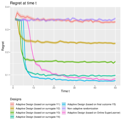
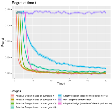
Figure 3: Regret at time $t$ for different design strategies in Scenario 1 (left) and Scenario 2 (right). This figure includes seven curves: five curves correspond to regrets from adaptive designs using outcomes from $Y_{1}$ to $Y_{5}$, respectively; one curve illustrates the regret for an adaptive design employing an Online Superlearner to evaluate and utilize surrogates; and the last curve represents the regret of a fixed design, which assigns equal probabilities to each treatment group.

Table 4: $R_{t,k}$ in Scenario 1 and 2 ($t=11,21,31,41,50$).

(a) Scenario 1 $t$ $R_{t,SL}$ $R_{t,RCT}$ $R_{t,1}$ $R_{t,2}$ $R_{t,3}$ $R_{t,4}$ $R_{t,5}$ 11 0.150 0.343 0.343 0.245 0.158 0.102 0.089 21 0.105 0.345 0.340 0.242 0.163 0.099 0.078 31 0.089 0.344 0.340 0.239 0.156 0.097 0.075 41 0.085 0.340 0.337 0.240 0.157 0.095 0.074 50 0.083 0.349 0.334 0.239 0.159 0.098 0.075

(b) Scenario 2 $t$ $R_{t,SL}$ $R_{t,RCT}$ $R_{t,1}$ $R_{t,2}$ $R_{t,3}$ $R_{t,4}$ $R_{t,5}$ 11 0.030 0.122 0.028 0.028 0.030 0.037 0.063 21 0.027 0.120 0.026 0.026 0.026 0.031 0.044 31 0.026 0.119 0.024 0.026 0.025 0.029 0.038 41 0.025 0.121 0.025 0.025 0.025 0.029 0.034 50 0.027 0.119 0.025 0.024 0.025 0.028 0.032

6 Extension and Discussion

In the adaptive design with the Online Superlearner, as investigated in previous sections, a conservative treatment randomization strategy is employed, ensuring that adaptations based on surrogate outcomes, as selected by the Online Superlearner, are initiated only subsequent to the observation of the primary outcome at $t=K+1$. However, there may be scenarios where experimenters wish to adapt treatment randomization probabilities at an earlier stage. To address this, we propose a modified strategy in which a plausible surrogate outcome (e.g., $Y_{k}$) is designated as a temporary primary outcome. This surrogate serves as the foundation for implementing our adaptive design that treats $Y_{k}$ as the primary outcome and enabling the adaptation of treatment randomization probabilities as early as $t=k+1$. As the experiment progresses, subsequent surrogate outcomes can be sequentially established as new temporary primary outcomes until the true primary outcome is observed. If one has prior knowledge or external datasets to infer the relationship between surrogates and primary outcomes, one can apply other methods to start adapting treatment randonmization probabilities earlier. However, that usually depends on generalization assumptions or prespecified models between surrogates and primary outcomes. We note that whatever strategy the experimenter chooses, our framework with Online Superlearner provides a tool for experimenters to evaluate how outcomes would be different under other designs that could have been implemented, and dynamically utilizes the most useful design within the ongoing sequential decision-making environment.

In summary, this manuscript contributes to both the fields of surrogate outcomes and adaptive designs in statistical research. We propose a novel target parameter to evaluate surrogate outcomes in the context of sequential adaptive designs. This parameter is defined as the counterfactual mean of the primary outcome of interest had each participant been treated, at their entry time, by stochastic rules that favor the optimal individualized treatment for the surrogate outcome under a counterfactual CARA design. Our target parameter not only emphasizes the evaluation of surrogates’ predictive precision regarding optimal individualized treatment rules for the primary outcome, but also quantifies the ability of surrogates to benefit more subjects at earlier stages through earlier shifts in randomization probability, providing a more comprehensive evaluation of surrogates’ benefits than alternative approaches. We further propose an adaptive design based on an online Superlearner to allow learning over the course of the study which of a set of candidate surrogates is most useful, and dynamically adapt subsequent randomization probabilities accordingly. This framework is widely applicable to evaluate a variety of adaptive designs distinguished by various characteristics, not limited to the surrogates they rely on for adapting randomization probabilities. While experimenters may only select a specific adaptive design at any given time, our evaluation framework provides a counterfactual reasoning approach to offer insights into how outcomes might differ under alternative design choices and converge over time, based on incoming data, to the best design for a given sequential decision-making process.

To address the issue of data dependency in adaptively collected data within CARA designs, we introduce Targeted Maximum Likelihood Estimation (TMLE) (Van der Laan et al., 2011; Van der Laan and Rose, 2018; van der Laan, 2008) to estimate the target parameter, obtaining a consistent and asymptotically normal estimator based on martingale CLT, fundamental maximal inqualities for martingale processes, and the recent theoretical results of Highly Adaptive Lasso (van der Laan, 2023). Our approach is broadly applicable for constructing robust estimators and providing statistical inference for a general class of context-specific causal parameters based on sequentially dependent data collected in multiple setups, including but not limited to adaptive sequential designs and time series with temporal dependence.

While we focus on the context-specific target parameter in this work, the comparison between this and the marginal parameter, as discussed in Remark 1, remains an interesting question in sequential decision-making setups. Research on this topic could provide valuable insights into the strengths and limitations of these parameters in answering causal queries, as well as the trade-offs with their statistical properties and computational efficiency in different scenarios. We leave the investigation of this topic for future research.

Appendix

Appendix A The Highly Adaptive Lasso Estimator

The Highly Adaptive Lasso (HAL) (van der Laan, 2015; Benkeser and van der Laan, 2016; van der Laan, 2023) is a nonparametric estimator for regression functions that does not require local smoothness of the true regression function. In short, the HAL estimator is constructed from a set of data-adaptive Càdlàg basis functions (i.e., right-hand continuous functions with left-hand limits) and is represented as the minimizer of an empirical risk criterion subject to a $L_{1}$ constraint on the sectional variation of the target regression function. In this paper, we use HAL to estimate Conditional Average Treatment Effect (CATE) functions (see Appendix B) and provide a corollary for proving equicontinuity condition of martingale process based on recent theoretical results of higher order spline HAL-MLEs in (van der Laan, 2023) (see Appendix C, D).

We first introduce $D^{(0)}([0,1]^{d})$, a class of $d$-variate cadlag functions defined on a unit cube $[0,1]^{d}$ with bounded sectional variation norm (Gill et al., 1995) and the Highly Adaptive Lasso Estimator for $D^{(0)}([0,1]^{d})$ (van der Laan, 2015; Benkeser and van der Laan, 2016; Bibaut and van der Laan, 2019). Then we will introduce the recent result of van der Laan (2023) that introduces $D^{(k)}([0,1]^{d})$ $(k=1,2,\cdots)$, a class of $k$-th order smoothness functions with bounded sectional variation norm on up to their $k$-th-order derivatives and the higher order spline HAL-MLEs to estimate them.

According to Gill et al. (1995); van der Laan (2015); Benkeser and van der Laan (2016), any function $Q\in D^{(0)}([0,1]^{d})$ can be represented as

$$Q(x)=\int_{[0,x]}dQ(u)=\int_{u\in[0,1]^{d}}\phi_{u}^{0}(x)dQ(u),$$

with basis function $\phi_{u}^{0}(x):=I(u\leq x)=\prod_{j=1}^{d}I\left(u_{j}\leq x_{j}\right)$ a tensor product of zero-order splines. For every non-empty $s\subset\{1,\ldots,d\}$, we can define $E_{s}=\left\{(x(s),0(-s)):x\in[0,1]^{d}\right\}$ as a $s$-specific zero edge of $[0,1]^{d}$, which sets the coordinates in the complement of subset $s$ equal to 0. As a convention, we include the empty subset $s=\emptyset$ in which case $E_{\emptyset}=\{0\}$. Since $[0,1]^{d}$ can be partitioned into the singleton $\{0\}$ ($s=\emptyset$), $s$-specific left-edges $E_{s}$ ($s\subsetneqq\{1,\ldots,d\}$, $s\neq\emptyset$), and the full-dimensional inner set $(0,1]^{d}$ ($s=\{1,\ldots,d\}$), one can represent $dQ(u)$ as the sum measure over these disjoint complementary supports $dQ(u)=\sum_{s\subset\{1,\ldots,d\}}I(u\in E_{s})dQ(u(s),0(-s))$. For $s=\emptyset$, $E_{s}=\{0\}$, $dQ(u(s),0(-s))=dQ(\{0\})=Q(0)$; for a non-empty $s\subsetneqq\{1,\ldots,d\}$, $dQ(u(s),0(-s))$ is the measure $Q(du(s),0(-s))$ implied by its $s$-specific section $Q_{s}:x(s)\to Q(x(s),0(-s))$ on the zero edge $E_{s}$; for $s=\{1,\ldots,d\}$, $dQ(u(s),0(-s))$ represents the measure for $u$ in the full-dimensional inner cube $(0,1]^{d}$. Therefore, any cadlag function $Q\in D^{(0)}([0,1]^{d})$ can also be written as

$$Q(x)=\int_{[0,x]}dQ(u):=Q(0)+\sum_{s\subset\{1,\ldots,d\},s\neq\emptyset}\int_{(0(s),x(s)]}Q(du(s),0(-s)).$$

The sectional variation norm of $Q$ is defined by the sum over $s$ of the variation norms of the measures on every $s$-specific section:

$$\|Q\|_{v}^{*}:=\int_{[0,1]^{d}}|dQ(u)|=|Q(0)|+\sum_{s\subset\{1,\ldots,d\},s\neq\emptyset}\int_{(0(s),1(s)]}|Q(du(s),0(-s))|.$$

We use $[d]$ to denote the full set $\{1,\ldots,d\}$ and correspondingly define $\mathcal{S}^{0}_{[d]}$ as the set of all subsets $s\subset[d]$, including the empty subset. For each subset $s\subset\{1,\ldots,d\}$, we define $\mathcal{R}^{0}(s)=(0(s),1(s)]$ on the $s$-specific zero edge $E_{s}$. Let $\mathcal{R}^{0}_{[d]}=\left\{(s,u_{s}):s\neq\emptyset,s\in\mathcal{S}^{0}_{[d]},u_{s}\in\mathcal{R}^{0}(s)\right\}\cup\left\{\left(\{0\},0\right):s=\emptyset\right\}$ be the set of all subsets $s\subset[d]$ and all knot points $u_{s}$ on $s$-specific zero edges, which represents all basis functions needed to span $D^{(0)}([0,1]^{d})$. Therefore, one can represent $D^{(0)}([0,1]^{d})$ by

$$D^{(0)}(\mathcal{R}^{0}_{[d]}):=\left\{\sum_{s\in\mathcal{S}^{0}_{[d]}}\int_{u_{s}\in\mathcal{R}^{0}(s)}\phi_{u_{s}}^{0}(\cdot)dQ(u_{s}):Q\in D^{(0)}([0,1]^{d})\right\}.$$

One can define $\mathcal{R}^{0,*}_{[d]}=\left\{(s,u_{s}):s\in\mathcal{S}^{0,*}_{[d]},u_{s}\in\mathcal{R}^{0,*}(s)\right\}$, where $\mathcal{S}^{0,*}_{[d]}\subset\mathcal{S}^{0}_{[d]}$ and $\mathcal{R}^{0,*}(s)\subset\mathcal{R}^{0}(s)$ for every $s\in[d]$. Since $\mathcal{R}^{0,*}_{[d]}$ is a subset of $\mathcal{R}^{0}_{[d]}$, one can define the following submodel of $D^{(0)}([0,1]^{d})$ based on $\mathcal{R}^{0,*}_{[d]}$:

$$D^{(0)}(\mathcal{R}^{0,*}_{[d]}):=\left\{\sum_{s\in\mathcal{S}^{0,*}_{[d]}}\int_{u_{s}\in\mathcal{R}^{0,*}(s)}\phi_{u_{s}}^{0}(\cdot)dQ(u_{s}):Q\in D^{(0)}([0,1]^{d})\right\}.$$

One can also specify a submodel whose sectional variation norm $\|Q\|_{v}^{*}$ is upper bounded by $C^{u}$:

$$D^{(0)}_{C^{u}}(\mathcal{R}^{0,*}_{[d]}):=\left\{\sum_{s\in\mathcal{S}^{0,*}_{[d]}}\int_{u_{s}\in\mathcal{R}^{0,*}(s)}\phi_{u_{s}}^{0}(\cdot)dQ(u_{s}):Q\in D^{(0)}([0,1]^{d}),\|Q\|_{v}^{*}<C^{u}\right\}.$$

Suppose we observe $n$ i.i.d samples $(x_{i},y_{i})$ ($i=1,\cdots,n$) with $x_{i}=(x_{i,1},\cdots,x_{i,d})\in\mathbb{R}^{d}$, $y_{i}\in\mathbb{R}$. van der Laan (2015); Benkeser and van der Laan (2016) proposed to use discrete measures that put mass on the observed knot points $\mathcal{R}_{n}^{0,*}(s)=(x_{i}(s),i\in[n])\subset\mathcal{R}^{0,*}(s)$ on all $s$-specific edges ($s\subset[d]$) to construct a submodel $D^{(0)}(\mathcal{R}^{0,n}_{[d]})$ to approximate the representation of $Q(x)$:

$$D^{(0)}(\mathcal{R}^{0,n}_{[d]}):=\left\{\sum_{s\in\mathcal{S}^{0,*}_{[d]}}\sum_{u_{s}\in\mathcal{R}_{n}^{0,*}(s)}\phi_{u_{s}}^{0}(\cdot)dQ(u_{s}):Q\in D^{(0)}([0,1]^{d})\right\},$$

where $\mathcal{R}^{0,n}_{[d]}:=\left\{(s,u_{s}):s\neq\emptyset,s\in\mathcal{S}^{0,*}_{[d]},u_{s}\in\mathcal{R}_{n}^{0,*}(s)\right\}\cup\left\{\left(\{0\},0\right):s=\emptyset\right\}$. Similarly, one can consider a submodel with bounded total variation norm $C^{u}$:

$$D^{(0)}_{C^{u}}(\mathcal{R}^{0,n}_{[d]}):=\left\{\sum_{s\in\mathcal{S}^{0,*}_{[d]}}\sum_{u_{s}\in\mathcal{R}_{n}^{0,*}(s)}\phi_{u_{s}}^{0}(\cdot)dQ(u_{s}):Q\in D^{(0)}([0,1]^{d}),\|Q\|_{v}^{*}<C^{u}\right\}.$$

Accordingly, a zero-order HAL-MLE can be defined by solving the following loss-based minimization problem:

$$Q_{n}=\mathop{\mathrm{argmin}}_{Q\in D^{(0)}_{C_{n}^{u}}(\mathcal{R}^{0,n}_{[d]})}\mathbb{P}_{n}L(Q),$$

with $L(\cdot)$ an appropriately defined loss function and $C_{n}^{u}$ a data-adaptive cross-validation or undersmoothed selector of bounded sectional variation norm for the working model. Define $\big{|}\mathcal{R}^{0,n}_{[d]}\big{|}$ the cardinality of $\mathcal{R}^{0,n}_{[d]}$ and $\mathcal{B}_{n}:=\left\{\beta:\beta\in\mathbb{R}^{\big{|}\mathcal{R}^{0,n}_{[d]}\big{|}};\beta=\left(\beta_{s,u_{s}}\right),(s,u_{s})\in\mathcal{R}_{n}^{0,*}(s)\right\}$. The construction of HAL-MLE is equivalent to solving

$$\beta_{n}=\mathop{\mathrm{argmin}}_{\beta:\beta\in\mathcal{B}_{n},\|\beta\|_{1}\leq C_{n}^{u}}\mathbb{P}_{n}L\left(\sum_{s\in\mathcal{S}^{0,*}_{[d]}}\sum_{u\in\mathcal{R}_{n}^{0,*}(s)}\phi_{u_{s}}^{0}(\cdot)\beta_{s,u_{s}}\right),$$

thus HAL-MLE can be expressed by $Q_{n}(\cdot)=\sum_{s\in\mathcal{S}^{0,*}_{[d]}}\sum_{u_{s}\in\mathcal{R}_{n}^{0,*}(s)}\phi_{u_{s}}^{0}(\cdot)\beta_{s,u_{s}}$. Bibaut and van der Laan (2019) shows the $L_{2}$ rate of convergence of $O(n^{-\frac{1}{3}})$ up till a $\log$-n factor for zero-order HAL-MLE.

van der Laan (2023) further defines a $k$-th order smoothness class $D^{(k)}([0,1]^{d})$ $(k=1,2,\cdots)$ on $[0,1]^{d}$, which includes functions $Q$ whose $k$-th-order Lebesgue Radon-Nikodym derivatives, defined on every nested subset $\bar{s}(k+1):=(s_{1},\cdots,s_{k+1})$ with $s_{k+1}\subset s_{k}\subset\cdots\subset s_{1}\subset[d]$, are real-valued cadlag function with bounded sectional variation norm for every nested subset $\bar{s}(k+1)$. Similar to representing $D^{(0)}([0,1]^{d})$ by sets of knot points $\mathcal{R}^{k,*}_{[d]}$ on each subset $s\subset[d]$, van der Laan (2023) shows that one can use knot points in $\mathcal{R}^{k,*}_{[d]}$ (an analogue to $\mathcal{R}^{0,*}_{[d]}$, including knot points $\mathcal{R}^{k,*}(\bar{s}(k+1))$ on nested subsets $\bar{s}(k+1)$) to represent $D^{(k)}([0,1]^{d})$, and use observed knot points $\mathcal{R}_{n}^{k,*}(\bar{s}(k+1))$ to construct a working model. Similar to the zero-order HAL MLE that estimates a target function in $D^{(0)}([0,1]^{d})$, one can construct a higher order HAL-MLE that uses $k$-th order splines to estimate the target function in $D^{(k)}([0,1]^{d})$. The $k$-th order HAL-MLEs are of form $Q_{n}(\cdot)=\sum_{\bar{s}(k+1)}\sum_{u\in\mathcal{R}_{n}^{k,*}(\bar{s}(k+1))}\phi_{u}^{k}(\cdot)\beta_{\bar{s}(k+1),u}$, with $\phi_{u}^{k}(\cdot):=\int_{u}^{x}\phi_{u_{1}}^{k-1}(\cdot)du_{1}$. For example, for $d=1$, the first-order spline function is $\phi^{1}_{u}(x)=(x-u)I(x\geq u)$, and second-order spline function for is $\phi^{2}_{u}(x)=\frac{1}{2}(x-u)^{2}I(x\geq u)$, and so on. van der Laan (2023) proved the supremum-norm covering number for $D^{(k)}([0,1]^{d})$ for $(k=1,2,\cdots)$, with a uniform entropy intergral $J_{\infty}\left(r,D^{(k)}([0,1]^{d})\right)\asymp r^{(2k+1)/(2k+2)}(-\log r)^{d-\frac{3}{2}}$. He also proved that the $k$-th order spline HAL-MLEs is asymptotically normal and has uniform rate of convergence of $n^{-\frac{k+1}{2k+3}}$ with up till $\log$ $n$-factors.

Appendix B Estimation of Conditional Average Treatment Effect

A key procedure in our adaptive design is estimating the Conditional Average Treatment Effect (CATE). By estimating the CATE function, the experimenter can identify the optimal treatment rule that maximizes the expected reward based on the expected outcome conditional on baseline covariates, and update treatment randomization probabilities in adaptive design as in Subsection 3.1.

We propose using the Highly Adaptive Lasso (HAL) estimator to estimate the CATE function. As introduced in Appendix A, the HAL estimator is a nonparametric regression method that can estimate a rich class of cadlag functions with a remarkable rate of convergence without relying on local smoothness assumptions. Furthermore, we can directly apply the delta-method to obtain a Wald-type confidence interval for the CATE. This confidence interval guides the exploration-exploitation trade-off in adaptive designs by adjusting treatment randomization probabilities based on the uncertainty in CATE estimates.

Recall that $\bar{Q}_{0,k}(A,W)=E[Y_{k}|A,W]$ is the true conditional expectation of the $k$-th surrogate outcome, given the treatment $A$ and baseline covariates $W$. For every new participant $i$ enrolled at time $t$, we use $B_{n,k,t}(w_{i})$ to denote an estimate of $B_{0,k}(w_{i})$ is the true CATE of $Y_{k}$ given $w_{i}$, the baseline covariates of participant $i$. We use $\tau_{n,k,t}(w_{i})$ to denote the estimated standard error of CATE. Both estimates are based on $\mathcal{H}(i)$, the historical data observed before participant $i$ is enrolled.

For each surrogate outcome $Y_{k}$, we estimate CATE functions by two steps. First, we transform $Y_{k}$ into the pseudo-outcome (Van der Laan, 2006; Luedtke and van der Laan, 2016):

$$\eta_{k}(\bar{Q}_{k},g)(O)=\frac{2A-1}{g(A\mid W)}[Y_{k}-\bar{Q}_{k}(A,W)]+\bar{Q}_{k}(1,W)-\bar{Q}_{k}(0,W).$$

We note that the pseudo-outcome has the double-robust property that $\mathbb{E}_{0}[\eta_{k}(\bar{Q}_{k},g)(O)\mid W]=B_{0,k}(W)$ if $\bar{Q}_{k}=\bar{Q}_{0,k}$ or $g=g_{0}$. Since $g_{0}$ is known in adaptive design, we only need to estimate $\bar{Q}_{0,k}$ with $\bar{Q}_{n,k}$, then impute $\bar{Q}_{n,k,t}$ and $g_{0}$ to generate the pseudo-outcome $\eta_{k}(\bar{Q}_{n,k,t},g_{0})$.

Second, we estimate the CATE function $B_{0,k}$ by regressing the pseudo-outcome $D_{k}\left(\bar{Q}_{n,k,t},g_{0}\right)$ on baseline covariates $W$ by first-order spline HAL-MLE, which minimizes the empirical risk over the $D^{(1)}([0,1]^{d})$,the first-order smoothness class with its first order derivative being cadlag function with bounded first order sectional variation norm. That is, at time $t$, we estimate the CATE function by solving the following minimization problem:

$$B_{n,k,t}=\mathop{\mathrm{argmin}}_{B_{k}\in D^{(1)}_{C_{n}^{u}}(\mathcal{R}^{1,n}_{[d]})}\frac{1}{n_{t,k}}\sum_{j=1}^{n_{t,k}}L_{k}(B_{k})(O_{j}),$$

where $L_{k}$ is the loss function defined by $L_{k}(B_{k})(O):=(B_{k}(W)-\eta_{k}(O))^{2}$; $n_{t,k}:=N(t-k)$ is the number of participants with observed $Y_{k}$ at time $t$; $\mathcal{R}^{1,n}_{[d]}$ is the set of observed knot points from samples (see Appendix A); $C_{n}^{u}$ is an upper bound for the first order sectional variation norm that is data-adaptively selected via cross-validation.

As introduced in Appendix A, $B_{n,k,t}(\cdot)$ can be written as a linear combination of first-order spline basis functions with non-zero coeffcients. To quantify the uncertainty of CATE estimates, we apply the delta method in this data-adaptive HAL working model to make inferences on CATE. We use $\tau_{n,k,t}(w_{i})$, the estimate of the standard error of $B_{n,k,t}(w_{i})$, to construct a Wald-type confidence interval for the CATE function. Both $B_{n,k,t}(w_{i})$ and $\tau_{n,k,t}(w_{i})$ are incorporated into the $h_{m}$ function in Section 3.1 to determine the treatment randomization probability $g_{k,i}^{*}$ for every participant $i$.

Appendix C General Theorem for Equicontinuity Condition of a General Martingale Process

In this section, we provide a theorem about the equicontinuity condition of martingale processes in a setup that is more general than our adaptive design.

C.1 Statistical Setup

Suppose we sequentially generate a sequence of data $O_{i}$ from $i=1$ to $N$. Every $O_{i}\in\mathcal{O}_{i}$ is generated from historical data $\bar{O}(i-1):=(O_{1},\cdots,O_{i-1})$. We define a probability triple $(\Omega,\mathcal{F},\mathbf{P})$, where $\mathcal{F}_{i}$, $(i=1,\cdots,N,\cdots)$ are defined as sub-sigma algebras $\mathcal{F}_{1}\subset\cdots\mathcal{F}_{N}\subset\cdots\subset\mathcal{F}$ with $\bar{O}(i)\in\mathcal{O}_{1}\times\cdots\times\mathcal{O}_{i}\subset\mathcal{F}_{i}$. We consider a scenario in which every $O_{i}$ is generated based on $\bar{O}(i-1)$ through a fixed dimensional summary measure $C_{i}\in\mathcal{C}$, where $C_{i}$ is generated by a known function $h_{C}:\bar{O}(i-1)\to\mathcal{C}$ for every $i=1,\cdots,N$.

Let $f_{\theta}:\mathcal{O}\times\mathcal{C}\to\mathbb{R}$ be a $\mathcal{F}_{i}$-measurable function, indexed by a class of functions $\Theta$. Define

$$M_{N}(\theta)=\frac{1}{N}\sum_{i=1}^{N}f_{\theta}(O_{i},C_{i})-E\left[f_{\theta}(O_{i},C_{i})\mid\bar{O}(i-1)\right].$$

Suppose there is an unknown element $\theta_{0}\in\Theta$ to be estimated by $\theta_{N}\in\Theta$ based on data $\bar{O}(N)$. We provide a general theorem for the equicontinuity condition with respect to the martingale process as follows:

$$M_{2,N}(\theta_{N},\theta_{0}):=M_{N}(\theta_{N})-M_{N}(\theta_{0})=o_{P}(N^{-\frac{1}{2}}).$$

C.2 Proof of Equicontinuity Condition

We first restate a bracketing entropy based on Definition A.1 in van Handel (2011) (which was introduced by Definition 8.1 in van de Geer (1999)) by our notation.

definitionrepDefSeqBracketing(Bracketing entropy for martingales) Consider a stochastic process of the form $\left\{\left(\xi_{\theta,i}\right)_{i=1}^{N}:\theta\in\Theta\right\}$ where $\Theta$ is an index set such that, for every $\theta\in\Theta,i\in[N]$, $\xi_{\theta,i}$ is an $\bar{O}(i)$-measurable random variable for all $i$ and $\theta$. Denote $F:=\bar{O}(N)\in\mathcal{F}$. We say that a collection of random variables of the form $\mathcal{B}:=\left\{\left(\Lambda_{i}^{j},\Upsilon_{i}^{j}\right)_{i=1}^{N}:j\in[J]\right\}$ is a $(N,\Theta,F,K,\epsilon)$-bracketing if

1. for every $i\in[N]$, and $j\in[J],\left(\Lambda_{i}^{j},\Upsilon_{i}^{j}\right)$ is $\bar{O}(i)$-measurable,

2. for every $\theta\in\Theta$, there exists $j\in[J]$, such that, for every $i\in[N],\Lambda_{i}^{j}\leq\xi_{\theta,i}\leq\Upsilon_{i}^{j}$,

3. for every $j\in[J]$,

   $$\frac{2K^{2}}{N}\sum_{i=1}^{N}E\left[\phi\left(\frac{\Upsilon_{i}^{j}-\Lambda_{i}^{j}}{K}\right)\mid\bar{O}(i-1)\right]\leq\epsilon^{2},$$

where $\phi(x)=e^{x}-x-1$. We denote $\mathcal{N}_{[]}\left(N,\Theta,F,{K},{\epsilon}\right)$ the minimal cardnality of an $\left(N,\Theta,\mathcal{F},K,\epsilon\right)$-bracketing. We define the bracketing entropy integral as $\mathcal{J}_{[]}\left(N,\Theta,F,{K},{\epsilon}\right):=\int_{0}^{\epsilon}\mathcal{N}_{[]}\left(N,\Theta,F,{K},{u}\right)du$.

Theorem 4 (Theorem A.4 in van Handel (2011)).

Given $K>0$, for all $i\geq 0$, define

$$M_{\theta,i}=\frac{1}{N}\sum_{l=1}^{i}\left(\xi_{\theta,l}-E\left[\xi_{\theta,l}\mid\mathcal{F}_{l-1}\right]\right),$$

$$R_{\theta,i}=\frac{1}{N}2K^{2}\sum_{l=1}^{i}E\left[\phi\left(\frac{|\xi_{\theta,l}|}{K}\right)\bigg{|}\mathcal{F}_{l-1}\right].$$

By Theorem A.4 in van Handel (2011), for any $N\in\mathbb{N}$, $x>0$, and $0<R<\infty$,

$$P\left(\sup_{\theta\in\Theta}I\left(R_{\theta,N}\leq R\right)\max_{i\in[N]}\sqrt{N}M_{\theta,i}\geq 16\mathcal{H}+32\sqrt{Rx}+\frac{16}{\sqrt{N}}Kx\right)\leq 2e^{-x},$$

where $\mathcal{H}:=\frac{K}{\sqrt{N}}\log\mathcal{N}_{[]}\left(N,\Theta,F,{K},{\sqrt{R}}\right)+4\mathcal{J}_{[]}\left(N,\Theta,F,{K},{\sqrt{R}}\right)$.

We focus on the process of $\xi_{\theta,i}=f_{\theta}(O_{i},C_{i})-f_{\theta_{0}}(O_{i},C_{i})$ ($i=1,\ldots,n$), with $\theta_{0}\in\Theta,\theta\in\Theta$. As the bracketing entropy condition may be hard to check because of its intricate definition, we relate it to the supremum norm covering entropy, following the approach outlined by van de Geer (1999) in Definition 8.1 and Chambaz and van der Laan (2011) in Lemma 7. Our method differs from their approaches in that we relate the bracketing entropy to the supremum norm covering entropy for $\Theta$ instead of $\{f_{\theta}:\theta\in\Theta\}$.

Let $\mathcal{N}_{\infty}\left({\epsilon},{\Theta}\right)$ denote the $\epsilon$-covering number in supremum norm of $\Theta$ and let $\mathcal{J}_{\infty}\left({\epsilon},{\Theta}\right):=\int_{0}^{\epsilon}\sqrt{\log\left(1+\mathcal{N}_{\infty}\left({\epsilon},{\Theta}\right)\right)}du$ denote the $\epsilon$-entropy integral in supremum norm of $\Theta$.

Assumption 5 (Uniform Boundedness).

$\sup_{\theta\in\Theta}\left\|\theta\right\|_{\infty}<\infty$, $\sup_{\theta\in\Theta}\left\|f_{\theta}\right\|_{\infty}<\infty$.

Assumption 6.

$\sup_{\theta_{1}\in\Theta,\theta_{2}\in\Theta,\theta_{1}\neq\theta_{2}}\frac{\left\|f_{\theta_{1}}-f_{\theta_{2}}\right\|_{\infty}}{\left\|\theta_{1}-\theta_{2}\right\|_{\infty}}<\infty$.

Lemma 1.

Suppose that Assumptions 5 and 6 hold and $N_{\infty}(\epsilon,\Theta)$ is finite. Then the following holds:

$$\mathcal{N}_{[]}\left(N,\Theta,F,{8mM},{2\sqrt{2}m\epsilon}\right)\leq\mathcal{N}_{\infty}(\epsilon,\Theta),$$

and

$$\mathcal{J}_{[]}\left(N,\Theta,F,{8mM},{2\sqrt{2}m\epsilon}\right)\leq\mathcal{J}_{\infty}\left({\epsilon},{\Theta}\right).$$

Proof.

Suppose $\{\theta_{j}:j\in[J]\}\subset\Theta$ is an $\epsilon$-covering of $\Theta$ in supremum norm such that $\forall\theta\in\Theta$, there exists $j\in[J]$ such that $\theta_{j}\in\Theta$ and $\|\theta_{j}-\theta\|_{\infty}\leq\epsilon$. Denoting $\lambda_{j}=\theta_{j}-\epsilon$ and $v_{j}=\theta_{j}+\epsilon$. Under Assumption 5, suppose $\left\|\theta\right\|_{\infty}<M$ for some $M>0$. Without loss of generality, we can suppose $\epsilon\leq 2M$ as $\lambda_{j}=\theta_{j}-M$ and $v_{j}=\theta_{j}+M$ always construct a valid pair of brackets. Under Assumption 6, suppose $\frac{\left\|f_{\theta_{1}}-f_{\theta_{2}}\right\|_{\infty}}{\left\|\theta_{1}-\theta_{2}\right\|_{\infty}}\leq m$, where $0<m<\infty$. Then $\left\|f_{\theta_{j}}-f_{\theta}\right\|_{\infty}\leq m\left\|\theta_{j}-\theta\right\|_{\infty}\leq m\epsilon$. Define $\Lambda_{i}^{j}=f_{\theta_{j}}-m\epsilon$ and $\Upsilon_{i}^{j}=f_{\theta_{j}}+m\epsilon$. Then $|\Upsilon_{i}^{j}-\Lambda_{i}^{j}|\leq 2m\epsilon$. Therefore, we have that

$$\frac{1}{N}2K^{2}\sum_{i=1}^{N}E\left[\phi\left(\frac{|\Upsilon_{i}^{j}-\Lambda_{i}^{j}|}{K}\right)\mid\bar{O}(i-1)\right]\leq 2K^{2}\phi\left(\frac{2m\epsilon}{K}\right)\leq 2K^{2}\sum_{p\geq 2}\frac{1}{p!}\frac{p!}{2}\left(\frac{2m\epsilon}{K}\right)^{p}=\frac{2m\epsilon}{\frac{1}{2m\epsilon}-\frac{1}{K}}.$$

Let $K=8mM$. We have that

$$\frac{1}{N}2K^{2}\sum_{i=1}^{N}E\left[\phi\left(\frac{|\Upsilon_{i}^{j}-\Lambda_{i}^{j}|}{K}\right)\mid\bar{O}(i-1)\right]\leq(2\sqrt{2}m\epsilon)^{2}.$$

Therefore,

$$\mathcal{N}_{[]}\left(N,\Theta,F,{8mM},{2\sqrt{2}m\epsilon}\right)\leq\mathcal{N}_{\infty}(\epsilon,\Theta),$$

and

$$\mathcal{J}_{[]}\left(N,\Theta,F,{8mM},{2\sqrt{2}m\epsilon}\right)\leq\mathcal{J}_{\infty}\left({\epsilon},{\Theta}\right).$$

∎

Assumption 7 (Convergence of $\theta_{N}$).

Define $\sigma_{N}\left(\theta,\theta_{0}\right):=\sqrt{\frac{1}{N}\sum_{i=1}^{N}E\left[\phi\left(\frac{f_{\theta}\left(O_{i},C_{i}\right)-f_{\theta_{0}}\left(O_{i},C_{i}\right)}{K}\right)\mid\bar{O}(i-1)\right]}$, where $K=8mM$. $\theta_{N}$ is an estimate of $\theta_{0}$ based on $\bar{O}(N)$ such that $\sigma_{N}\left(\theta_{N},\theta_{0}\right)=o_{P}(1)$.

Theorem 5 (Maximal Inequality of Martingale Process).

$\forall x>0,N\in\mathbb{N}$, and $0<r<\infty$. Denote $a_{N}(r,x):=\frac{16K}{\sqrt{N}}\log\mathcal{N}_{\infty}\left({\frac{r}{2\sqrt{2}m}},{\Theta}\right)+64\mathcal{J}_{\infty}\left({\frac{r}{2\sqrt{2}m}},{\Theta}\right)+32r\sqrt{x}+\frac{16}{\sqrt{N}}Kx$. Suppose that Assumptions 5, 6 and 7 hold. Then,

$$P\left(\sup_{\theta_{0}\in\Theta}I\left(\sigma_{N}(\theta_{N},\theta_{0})\leq r\right)\sqrt{N}M_{2,N}(\theta_{N},\theta_{0})\geq a_{N}(r,x)\right)\leq 2e^{-x}.$$

Proof.

Recall that

$$M_{2,N}(\theta_{N},\theta_{0})=\frac{1}{N}\sum_{i=1}^{N}f_{\theta}\left(O_{i},C_{i}\right)-f_{\theta_{0}}\left(O_{i},C_{i}\right)-E\left[f_{\theta}(O_{i},C_{i})-f_{\theta_{0}}(O_{i},C_{i})\mid\bar{O}(i-1)\right].$$

Let $K=8mM$ and $b_{N}(r,x)=\frac{16K}{\sqrt{N}}\log\mathcal{N}_{[]}\left(N,\Theta,F,{K},{r}\right)+64\mathcal{J}_{[]}\left(N,\Theta,F,{K},{r}\right)+32r\sqrt{x}+\frac{16}{\sqrt{N}}Kx$. We have that

$$P\left(\sqrt{N}M_{2,N}(\theta_{N},\theta_{0})I\left(\sigma_{N}\left(\theta_{N},\theta_{0}\right)\leq r\right)\geq a_{N}(r,x)\right) \leq P\left(\sup_{\theta_{0}\in\Theta}I\left(\sigma_{\theta,N}\leq r\right)\sqrt{N}M_{2,N}(\theta_{N},\theta_{0})\geq a_{N}(r,x)\right)$$

$$\leq P\left(\sup_{\theta_{0}\in\Theta}I\left(\sigma_{\theta,N}\leq r\right)\sqrt{N}M_{2,N}(\theta_{N},\theta_{0})\geq b_{N}(r,x)\right)$$

$$\leq 2e^{-x},$$

where the second inequality is given by Lemma 1 and the third inequality is based on the maximal inequality for the martingale process in Theorem 4.

∎

corollaryrepCoroHighOrderSplineEquicontinuity_general Suppose Assumptions 5, 6 and 7 hold, then $M_{2,N}(\theta_{N},\theta_{0})=o_{P}(N^{-\frac{1}{2}})$.

Proof.

Let $r_{N}$ to be any sequence that converges to 0 at a rate slower than $\sigma_{N}(\theta_{N},\theta_{0})$ does as $N\to\infty$. $\forall x>0,y>0$. Since

$$a_{N}(r_{N},x) =\frac{16K}{\sqrt{N}}\log\mathcal{N}_{\infty}\left({\frac{r_{N}}{2\sqrt{2}m}},{\Theta}\right)+64\mathcal{J}_{\infty}\left({\frac{r_{N}}{2\sqrt{2}m}},{\Theta}\right)+32r_{N}\sqrt{x}+\frac{16}{\sqrt{N}}Kx$$

$$\leq\frac{16K}{\sqrt{N}}\left(\frac{2\sqrt{2}m}{r_{N}}\mathcal{J}_{\infty}\left({\frac{r_{N}}{2\sqrt{2}m}},{\Theta}\right)\right)^{2}+64\mathcal{J}_{\infty}\left({\frac{r_{N}}{2\sqrt{2}m}},{\Theta}\right)+32r_{N}\sqrt{x}+\frac{16}{\sqrt{N}}Kx$$

$$\leq\left(\frac{108m^{2}K}{\sqrt{N}r_{N}^{2}}\mathcal{J}_{\infty}\left({\frac{r_{N}}{2\sqrt{2}m}},{\Theta}\right)+64\right)\mathcal{J}_{\infty}\left({\frac{r_{N}}{2\sqrt{2}m}},{\Theta}\right)+32r_{N}\sqrt{x}+\frac{16}{\sqrt{N}}Kx$$

$$\to 0,$$

there exists a $N_{1}>0$, such that for every $N>N_{1}$,

$$P(\sqrt{N}M_{2,N}(\theta_{N},\theta_{0})I\left(\sigma_{N}\left(\theta_{N},\theta_{0}\right)\leq r_{N}\right)>y)$$

$$\leq P\left(\sup_{\theta_{0}\in\Theta}I\left(\sigma_{\theta,N}\leq r_{N}\right)\sqrt{N}M_{2,N}(\theta_{N},\theta_{0})\geq a_{N}(r_{N},x)\right)$$

$$\leq 2e^{-x},$$

with the last inequality implied by Theorem 5. Similarly, $\forall x>0,y>0$, there exists a $N_{2}>0$, such that for every $N>N_{2}$, $P(-\sqrt{N}M_{2,N}(\theta_{N},\theta_{0})I\left(\sigma_{N}\left(\theta_{N},\theta_{0}\right)\leq r_{N}\right)>y)\leq 2e^{-x}$. Combined with Assumption 7 which implies $P(\sigma_{N}\left(\theta_{N},\theta_{0}\right)\leq r_{N})\to 1$, we have that $\sqrt{N}M_{2,N}(\theta_{N},\theta_{0})=o_{P}(1).$ ∎

As introduced in Appendix A, van der Laan (2023) proved the supremum-norm covering number for the class of functions $D^{(k)}([0,1]^{d})$ for $(k=1,2,\cdots)$, which implies a bound on its uniform entropy intergral $J_{\infty}\left(r,D^{(k)}([0,1]^{d})\right)\asymp r^{(2k+1)/(2k+2)}(-\log r)^{d-\frac{3}{2}}$. He also defined the $k$-th order HAL-MLEs and proved that their uniform rate of convergence is $N^{-\frac{k+1}{2k+3}}$ with up till $\log$ $N$-factors. Using these theoretical results, we provide another corollary which shows that if the target function $\theta_{0}$ lies in $D^{(k)}([0,1]^{d})$ ($k=1,2,3,\cdots$) and $\theta_{N}$ is an estimate of $\theta_{0}$ by higher order spline HAL-MLE, then the equicontinuity result for the martingale process $M_{2,N}$ holds.

assumptionrepAssmpHigherOrderSpline_general Suppose that $\theta_{0}\in D^{(k)}([0,1]^{d})$ and $\theta_{N}$ is estimated by the $k$-order spline HAL-MLE $(k=1,2,\cdots)$.

corollaryrepCoroHighOrderSplineEquicontinuity_general Suppose Assumptions 5, 6 and 5 hold, then $M_{2,N}(\theta_{N},\theta_{0})=o_{P}(N^{-\frac{1}{2}})$.

Proof.

Let $N_{\infty}\left(r,D^{(k)}([0,1]^{d})\right)$ denote the number of spheres of size $\epsilon$ w.r.t. supremum norm that are needed to cover $D^{(k)}([0,1]^{d})$. Define $J_{\infty}\left(r,D^{(k)}([0,1]^{d})\right)$ as the corresponding supremum norm entropy integral of $D^{(k)}([0,1]^{d})$. In van der Laan (2023), Lemma 29 shows that $J_{\infty}\left(r,D^{(k)}([0,1]^{d})\right)\asymp r^{(2k+1)/(2k+2)}(-\log r)^{d-\frac{3}{2}}$; Theorem 12 proves the uniform convergence rate $\left\|\theta_{N}-\theta_{0}\right\|_{\infty}=O_{P}(N^{-\frac{k+1}{2k+3}}\log^{m_{1}}N)$ for some specified $m_{1}<\infty$, which satisfies Assumption 7 that $\sigma_{N}(\theta_{N},\theta_{0})=o_{P}(1)$. Therefore, if Assumption 5 and 6 also hold, one can apply Corollary 5 to prove that $M_{2,N}(\theta_{N},\theta_{0})=o_{P}(N^{-\frac{1}{2}})$. ∎

Appendix D Proof of Equicontinuity Result in Adaptive Designs

Recall that the equicontinuity term in Section 4 is

$$M_{2,N}\left(\bar{Q}_{N,K}^{*},\bar{Q}_{0,K}\right) =\frac{1}{N}\sum_{i=1}^{N}\Biggl{\{}\biggl{[}D_{k}\left(\bar{Q}_{N,K}^{*}\right)\left(O_{i},C_{i}\right)-E\left[D_{k}\left(\bar{Q}_{N,K}^{*}\right)\left(O_{i},C_{i}\right)|\mathcal{H}(i)\right]\biggr{]}$$

$$-\biggl{[}D_{k}\left(\bar{Q}_{0,K}\right)\left(O_{i},C_{i}\right)-E\left[D_{k}\left(\bar{Q}_{0,K}\right)\left(O_{i},C_{i}\right)|\mathcal{H}(i)\right]\biggr{]}\Biggr{\}}.$$

where $D_{k}(\bar{Q}_{K})\left(O_{i},C_{i}\right):=\frac{g^{*}_{k,i}\left(A_{i}|C_{i}\right)}{g_{0,i}\left(A_{i}|C_{i}\right)}\left(Y_{i,K}-\bar{Q}_{K}\left(A_{i},W_{i}\right)\right)$. We apply the general results in Appendix C to prove the equicontinuity condition $M_{2,N}(\bar{Q}_{N,K}^{*},\bar{Q}_{0,K})=o_{P}(N^{-\frac{1}{2}})$ in Theorem 4.2 and Corollary 4.2 in the context of adaptive designs.

Proof of Theorem 4.2 and Corollary 4.2.

Let $\Theta:=\bar{\mathcal{Q}}_{K}$, $f_{\theta}:=D_{k}(\bar{Q}_{K})$, $\theta_{0}:=\bar{\mathcal{Q}}_{0,K}$, $\theta_{N}:=\bar{\mathcal{Q}}_{N,K}$ in the general setup in Appendix C. Under Assumption 3, $\zeta<g_{0,i}<1-\zeta$ and $\zeta<g_{k,i}^{*}<1-\zeta$. Since $Y_{K}$ and $Q_{K}$ take values in the interval $[0,1]$, we have that $\sup_{\bar{Q}_{K}\in\bar{\mathcal{Q}}_{K}}\left\|D_{k}(\bar{Q}_{K})\right\|_{\infty}\leq\frac{2(1-\zeta)}{\zeta}<\infty$, $\sup_{\bar{Q}_{K,1}\in\bar{\mathcal{Q}}_{K},\bar{Q}_{K,2}\in\bar{\mathcal{Q}}_{K},\bar{Q}_{K,1}\neq\bar{Q}_{K,2}}\frac{\left\|D_{k}(\bar{Q}_{K,1})-D_{k}(\bar{Q}_{K,2})\right\|_{\infty}}{\left\|\bar{Q}_{K,1}-\bar{Q}_{K,2}\right\|_{\infty}}\leq\frac{1-\zeta}{\zeta}<\infty$. Therefore, Assumptions 5 and 6 are satisfied. Since Assumption 4.2 serves as an analog in our adaptive design framework to Assumption 7 in the general framework, we can utilize Corollary 5 to demonstrate that $M_{2,N}\left(\bar{Q}_{N,K}^{*},\bar{Q}_{0,K}\right)=o_{P}(N^{-\frac{1}{2}})$. Similarly, Assumption 4.2 parallels Assumption 5 in Corollary 5. Therefore, Corollary 4.2 is a specification of Corollary 5 within our adaptive design setup. ∎

References

- Atkinson et al. (2011) AC Atkinson, A Biswas, and L Pronzato. Covariate-balanced response-adaptive designs for clinical trials with continuous responses that target allocation probabilities. Technical report, Technical Report NI11042-DAE, Isaac Newton Institute for Mathematical …, 2011.
- Benkeser and van der Laan (2016) David Benkeser and Mark van der Laan. The highly adaptive lasso estimator. In 2016 IEEE international conference on data science and advanced analytics (DSAA), pages 689–696. IEEE, 2016.
- Bibaut et al. (2021) Aurélien Bibaut, Maria Dimakopoulou, Nathan Kallus, Antoine Chambaz, and Mark van Der Laan. Post-contextual-bandit inference. Advances in neural information processing systems, 34:28548–28559, 2021.
- Bibaut and van der Laan (2019) Aurélien F Bibaut and Mark J van der Laan. Fast rates for empirical risk minimization over cadlag functions with bounded sectional variation norm. arXiv preprint arXiv:1907.09244, 2019.
- Breiman (2001) Leo Breiman. Random forests. Machine learning, 45:5–32, 2001.
- Brown (1971) Bruce M Brown. Martingale central limit theorems. The Annals of Mathematical Statistics, pages 59–66, 1971.
- Bubeck et al. (2012) Sébastien Bubeck, Nicolo Cesa-Bianchi, et al. Regret analysis of stochastic and nonstochastic multi-armed bandit problems. Foundations and Trends® in Machine Learning, 5(1):1–122, 2012.
- Buyse et al. (2000) Marc Buyse, Geert Molenberghs, Tomasz Burzykowski, Didier Renard, and Helena Geys. The validation of surrogate endpoints in meta-analyses of randomized experiments. Biostatistics, 1(1):49–67, 2000.
- Chambaz and van der Laan (2011) Antoine Chambaz and Mark J van der Laan. Targeting the optimal design in randomized clinical trials with binary outcomes and no covariate: simulation study. The International Journal of Biostatistics, 7(1), 2011.
- Chambaz and van der Laan (2014) Antoine Chambaz and Mark J van der Laan. Inference in targeted group-sequential covariate-adjusted randomized clinical trials. Scandinavian Journal of Statistics, 41(1):104–140, 2014.
- Chambaz et al. (2017) Antoine Chambaz, Wenjing Zheng, and Mark J van der Laan. Targeted sequential design for targeted learning inference of the optimal treatment rule and its mean reward. Annals of statistics, 45(6):2537, 2017.
- Chen and Guestrin (2016) Tianqi Chen and Carlos Guestrin. Xgboost: A scalable tree boosting system. In Proceedings of the 22nd acm sigkdd international conference on knowledge discovery and data mining, pages 785–794, 2016.
- Chow and Chang (2008) Shein-Chung Chow and Mark Chang. Adaptive design methods in clinical trials–a review. Orphanet journal of rare diseases, 3(1):1–13, 2008.
- Daniels and Hughes (1997) Michael J Daniels and Michael D Hughes. Meta-analysis for the evaluation of potential surrogate markers. Statistics in medicine, 16(17):1965–1982, 1997.
- Duan et al. (2021) Weitao Duan, Shan Ba, and Chunzhe Zhang. Online experimentation with surrogate metrics: Guidelines and a case study. In Proceedings of the 14th ACM International Conference on Web Search and Data Mining, pages 193–201, 2021.
- Elliott (2023) Michael R Elliott. Surrogate endpoints in clinical trials. Annual Review of Statistics and its Application, 10:75–96, 2023.
- Frangakis and Rubin (2002) Constantine E Frangakis and Donald B Rubin. Principal stratification in causal inference. Biometrics, 58(1):21–29, 2002.
- Freedman et al. (1992) Laurence S Freedman, Barry I Graubard, and Arthur Schatzkin. Statistical validation of intermediate endpoints for chronic diseases. Statistics in medicine, 11(2):167–178, 1992.
- Gilbert and Hudgens (2008) Peter B Gilbert and Michael G Hudgens. Evaluating candidate principal surrogate endpoints. Biometrics, 64(4):1146–1154, 2008.
- Gill et al. (1995) Richard D Gill, Mark J Laan, and Jon A Wellner. Inefficient estimators of the bivariate survival function for three models. In Annales de l’IHP Probabilités et statistiques, volume 31, pages 545–597, 1995.
- Hadad et al. (2021) Vitor Hadad, David A Hirshberg, Ruohan Zhan, Stefan Wager, and Susan Athey. Confidence intervals for policy evaluation in adaptive experiments. Proceedings of the national academy of sciences, 118(15):e2014602118, 2021.
- Hsu et al. (2015) Jesse Y Hsu, Edward H Kennedy, Jason A Roy, Alisa J Stephens-Shields, Dylan S Small, and Marshall M Joffe. Surrogate markers for time-varying treatments and outcomes. Clinical Trials, 12(4):309–316, 2015.
- Hu and Rosenberger (2006) Feifang Hu and William F Rosenberger. The theory of response-adaptive randomization in clinical trials. John Wiley & Sons, 2006.
- Huang et al. (2009) Xuelin Huang, Jing Ning, Yisheng Li, Elihu Estey, Jean-Pierre Issa, and Donald A Berry. Using short-term response information to facilitate adaptive randomization for survival clinical trials. Statistics in medicine, 28(12):1680–1689, 2009.
- Joffe and Greene (2009) Marshall M Joffe and Tom Greene. Related causal frameworks for surrogate outcomes. Biometrics, 65(2):530–538, 2009.
- Lattimore and Szepesvári (2020) Tor Lattimore and Csaba Szepesvári. Bandit algorithms. Cambridge University Press, 2020.
- Lin et al. (1997) DY Lin, TR Fleming, and V De Gruttola. Estimating the proportion of treatment effect explained by a surrogate marker. Statistics in medicine, 16(13):1515–1527, 1997.
- Luedtke and Van Der Laan (2016) Alexander R Luedtke and Mark J Van Der Laan. Statistical inference for the mean outcome under a possibly non-unique optimal treatment strategy. Annals of statistics, 44(2):713, 2016.
- Luedtke and van der Laan (2016) Alexander R Luedtke and Mark J van der Laan. Super-learning of an optimal dynamic treatment rule. The international journal of biostatistics, 12(1):305–332, 2016.
- Malenica et al. (2021) Ivana Malenica, Aurelien Bibaut, and Mark J van der Laan. Adaptive sequential design for a single time-series. arXiv preprint arXiv:2102.00102, 2021.
- Malenica et al. (2024) Ivana Malenica, Jeremy R Coyle, Mark J van der Laan, and Maya L Petersen. Adaptive sequential surveillance with network and temporal dependence. Biometrics, 80(1):ujad007, 2024.
- McDonald et al. (2023) Thomas M McDonald, Lucas Maystre, Mounia Lalmas, Daniel Russo, and Kamil Ciosek. Impatient bandits: Optimizing recommendations for the long-term without delay. In Proceedings of the 29th ACM SIGKDD Conference on Knowledge Discovery and Data Mining, pages 1687–1697, 2023.
- Montoya et al. (2021) Lina Montoya, Mark van der Laan, Alexander Luedtke, Jennifer Skeem, Jeremy Coyle, and Maya Petersen. The optimal dynamic treatment rule superlearner: considerations, performance, and application. arXiv preprint arXiv:2101.12326, 2021.
- Murphy (2003) Susan A Murphy. Optimal dynamic treatment regimes. Journal of the Royal Statistical Society Series B: Statistical Methodology, 65(2):331–355, 2003.
- Pearl et al. (2000) Judea Pearl et al. Models, reasoning and inference. Cambridge, UK: CambridgeUniversityPress, 19(2):3, 2000.
- Prentice (1989) Ross L Prentice. Surrogate endpoints in clinical trials: definition and operational criteria. Statistics in medicine, 8(4):431–440, 1989.
- Richardson et al. (2023) Lee Richardson, Alessandro Zito, Dylan Greaves, and Jacopo Soriano. Pareto optimal proxy metrics. arXiv preprint arXiv:2307.01000, 2023.
- Robbins (1952) Herbert Robbins. Some aspects of the sequential design of experiments. 1952.
- Robertson et al. (2023) David S Robertson, Kim May Lee, Boryana C López-Kolkovska, and Sofía S Villar. Response-adaptive randomization in clinical trials: from myths to practical considerations. Statistical science: a review journal of the Institute of Mathematical Statistics, 38(2):185, 2023.
- Robins (1986) James Robins. A new approach to causal inference in mortality studies with a sustained exposure period—application to control of the healthy worker survivor effect. Mathematical modelling, 7(9-12):1393–1512, 1986.
- Robins (1987) James M Robins. Addendum to “a new approach to causal inference in mortality studies with a sustained exposure period—application to control of the healthy worker survivor effect”. Computers & Mathematics with Applications, 14(9-12):923–945, 1987.
- Robins and Greenland (1992) James M Robins and Sander Greenland. Identifiability and exchangeability for direct and indirect effects. Epidemiology, 3(2):143–155, 1992.
- Rosenberger and Lachin (2015) William F Rosenberger and John M Lachin. Randomization in clinical trials: theory and practice. John Wiley & Sons, 2015.
- Rosenberger and Sverdlov (2008) William F Rosenberger and Oleksandr Sverdlov. Handling covariates in the design of clinical trials. 2008.
- Rosenberger et al. (2001) William F Rosenberger, AN Vidyashankar, and Deepak K Agarwal. Covariate-adjusted response-adaptive designs for binary response. Journal of biopharmaceutical statistics, 11(4):227–236, 2001.
- Simchi-Levi and Wang (2023) David Simchi-Levi and Chonghuan Wang. Multi-armed bandit experimental design: Online decision-making and adaptive inference. In International Conference on Artificial Intelligence and Statistics, pages 3086–3097. PMLR, 2023.
- Tamura et al. (1994) Roy N Tamura, Douglas E Faries, John S Andersen, and John H Heiligenstein. A case study of an adaptive clinical trial in the treatment of out-patients with depressive disorder. Journal of the American Statistical Association, pages 768–776, 1994.
- Thompson (1933) William R Thompson. On the likelihood that one unknown probability exceeds another in view of the evidence of two samples. Biometrika, 25(3-4):285–294, 1933.
- van de Geer (1999) S.A. van de Geer. Applications of Empirical Process Theory. Cambridge series in statistical and probabilistic mathematics. Cambridge U.P., 1999. URL https://books.google.com/books?id=Naq0swEACAAJ.
- van der Laan (2017) Mark van der Laan. A generally efficient targeted minimum loss based estimator based on the highly adaptive lasso. The international journal of biostatistics, 13(2), 2017.
- van der Laan (2023) Mark van der Laan. Higher order spline highly adaptive lasso estimators of functional parameters: Pointwise asymptotic normality and uniform convergence rates. arXiv preprint arXiv:2301.13354, 2023.
- Van der Laan (2006) Mark J Van der Laan. Statistical inference for variable importance. The International Journal of Biostatistics, 2(1), 2006.
- van der Laan (2008) Mark J van der Laan. The construction and analysis of adaptive group sequential designs. 2008.
- van der Laan (2015) Mark J van der Laan. A generally efficient targeted minimum loss based estimator. 2015.
- van der Laan and Luedtke (2015) Mark J van der Laan and Alexander R Luedtke. Targeted learning of the mean outcome under an optimal dynamic treatment rule. Journal of causal inference, 3(1):61–95, 2015.
- van der Laan and Malenica (2018) Mark J van der Laan and Ivana Malenica. Robust estimation of data-dependent causal effects based on observing a single time-series. arXiv preprint arXiv:1809.00734, 2018.
- Van der Laan and Rose (2018) Mark J Van der Laan and Sherri Rose. Targeted learning in data science. Springer, 2018.
- Van Der Laan and Rubin (2006) Mark J Van Der Laan and Daniel Rubin. Targeted maximum likelihood learning. The international journal of biostatistics, 2(1), 2006.
- Van der Laan et al. (2007) Mark J Van der Laan, Eric C Polley, and Alan E Hubbard. Super learner. Statistical applications in genetics and molecular biology, 6(1), 2007.
- Van der Laan et al. (2011) Mark J Van der Laan, Sherri Rose, et al. Targeted learning: causal inference for observational and experimental data, volume 4. Springer, 2011.
- van der Laan et al. (2022) Mark J van der Laan, David Benkeser, and Weixin Cai. Efficient estimation of pathwise differentiable target parameters with the undersmoothed highly adaptive lasso. The International Journal of Biostatistics, (0), 2022.
- van Handel (2011) Ramon van Handel. On the minimal penalty for markov order estimation. Probability theory and related fields, 150:709–738, 2011.
- VanderWeele (2013) Tyler J VanderWeele. Surrogate measures and consistent surrogates. Biometrics, 69(3):561–565, 2013.
- Weir and Taylor (2022) Christopher J Weir and Rod S Taylor. Informed decision-making: Statistical methodology for surrogacy evaluation and its role in licensing and reimbursement assessments. Pharmaceutical Statistics, 21(4):740–756, 2022.
- Yang et al. (2023) Jeremy Yang, Dean Eckles, Paramveer Dhillon, and Sinan Aral. Targeting for long-term outcomes. Management Science, 2023.
- Zhan et al. (2021) Ruohan Zhan, Vitor Hadad, David A Hirshberg, and Susan Athey. Off-policy evaluation via adaptive weighting with data from contextual bandits. In Proceedings of the 27th ACM SIGKDD Conference on Knowledge Discovery & Data Mining, pages 2125–2135, 2021.
- Zhang et al. (2007) Li-Xin Zhang, Feifang Hu, Siu Hung Cheung, and Wai Sum Chan. Asymptotic properties of covariate-adjusted response-adaptive designs. 2007.
- Zheng and Van Der Laan (2010) Wenjing Zheng and Mark J Van Der Laan. Asymptotic theory for cross-validated targeted maximum likelihood estimation. 2010.
- Zhu (2015) Hongjian Zhu. Covariate-adjusted response adaptive designs incorporating covariates with and without treatment interactions. Canadian Journal of Statistics, 43(4):534–553, 2015.