On the Infinite-Nudging Limit of the Nudging Filter for Continuous Data Assimilation

Abstract.

This article studies the intimate relationship between two filtering algorithms for continuous data assimilation, the synchronization filter and the nudging filter, in the paradigmatic context of the two-dimensional (2D) Navier-Stokes equations (NSE) for incompressible fluids. In this setting, the nudging filter can formally be viewed as an affine perturbation of the 2D NSE. Thus, in the degenerate limit of zero nudging parameter, the nudging filter converges to the solution of the 2D NSE. However, when the nudging parameter of the nudging filter is large, the perturbation becomes singular. It is shown that in the singular limit of infinite nudging parameter, the nudging filter converges to the synchronization filter. In establishing this result, the article fills a notable gap in the literature surrounding these algorithms. Numerical experiments are then presented that confirm the theoretical results and probes the issue of selecting a nudging strategy in the presence of observational noise. In this direction, an adaptive nudging strategy is proposed that leverages the insight gained from the relationship between the synchronization filter and the nudging filter that produces measurable improvement over the constant nudging strategy.

Keywords: continuous data assimilation, nudging filter, synchronization filter, Navier-Stokes equations, infinite nudging, singular limit, adaptive nudging, optimal nudging
MSC 2010 Classifications: 35Q30, 35B30, 37L15, 76B75, 76D05, 93B52

1. Introduction

Data assimilation (DA) was born in the 1960s, when it was proposed by J. Charney, M. Halem, and R. Jastrow [CHJ69] that the equations of motion of the atmosphere be used to process observations collected on the evolving state of the atmosphere for the purpose of improving their prognostic capabilities. Preceding [CHJ69], it was proposed in a milestone paper of V. Bjerknes [Bje04] that the problem of weather prediction be reduced to the direct numerical simulation of the equations of motion and the obtaining of a sufficiently accurate approximation of the state of the atmosphere with which to initialize the equations. It was in the advent of scientific computing in the 1950s [CFVN50, Cha51] and launch of the first weather satellites in the 1960s [Kal03] that DA was conceived in the spirit of the mechanistic perspective to meteorology of Bjerknes. Although numerical weather prediction continues to be an important application of DA, DA methods have since become essential in any situation for which both a model and observations on the modeled phenomenon are available.

Two fundamental issues in the study of DA derive from the nonlinear and high-dimensional nature of the model of interest, as well as the presence of errors in both the model and observations. Since the seminal work of R.E. Kalman and R.S. Bucy [KB61], it has been known that when the system is linear and errors are Gaussian, the optimal predictive process is also linear and Gaussian. Thus, any situation in which the underlying system is nonlinear must naturally contend with non-Gaussianity, leading to issues in sampling and efficient computation. Perhaps more importantly, the results in [KB61] indicated that new methods were required to account for nonlinearity appropriately. Many important efforts have subsequently been dedicated to addressing these issues; the reader is referred to the following seminal works [Lor86, LDT86, GSS93, Eve97, BvLG98] and the review articles [Kün13, CBBE18, PVS22]. On the other hand, in many applications, the model of interest is often given by a nonlinear system of partial differential equations (PDEs). Thus, a deeper understanding of DA methods is inevitably rooted in the understanding of how the incorporation of observations interact with nonlinearity in PDEs; this article is a contribution to the latter endeavor.

In particular, the primary concern of this paper is to establish a rigorous theoretical relationship between two filtering algorithms for CDA, the synchronization filter and the nudging filter. The study of these algorithms is carried out under the mathematically ideal assumptions of the availability of a perfect model, given by a dissipative partial differential equation (PDE), and noise-free observations, so that the fundamental issues of nonlinearity and high-dimensionality are isolated from the issues involved with the presence of noise. Naturally, the important issue of the effect of observational or model errors must be addressed in a subsequent study. This work may nevertheless be considered as a foundational step in bridging our understanding of these two algorithms. In this direction, the reader is also referred to a recent work of the authors [CFMV24] in which the precise relationship between the determining modes property, synchronization filter, and nudging filter is established through the notion of intertwinement.

The particular model we consider is the Navier-Stokes equations (NSE) for incompressible fluids in two-dimensions (2D), which has been used as a paradigmatic example for CDA studies [AJSV08, SAS15] due to its connection as a model for turbulent fluid flow, a phenomenon that exhibits a large number of degrees of freedom and chaotic dynamical behavior [FT87, FMRT01]. We will specifically consider the 2D NSE over a rectangular spatial domain, $\Omega=[0,2\pi]^{2}$, equipped with periodic boundary conditions for analytic convenience:

$$\partial_{t}u+u\cdotp\nabla u=-\nabla p+\nu\Delta u+f,\quad\nabla\cdotp u=0.$$ (1.1)

where $u=(u^{1},u^{2})$ denotes the velocity vector field, $\nu$ the kinematic viscosity, $p$ the scalar pressure field, and $f$ a given external force which is used to sustain turbulent behavior of the modeled fluid. We denote solutions to the corresponding initial value problem of (1.1) by $u(\cdotp;u_{0})$, where $u(0;u_{0})=u_{0}$. In the analysis of (1.1), it is customary to apply the Leray projection onto divergence-free vector fields to (1.1) and subsequently consider the equivalent functional formulation of (1.1) given as

$$\frac{du}{dt}+\nu Au+B(u,u)=Pf,$$ (1.2)

where $P$ denotes the Leray projection onto divergence-free vector fields, $A=-P\Delta$ is the Stokes operator, and $B$ is the bilinear form defined by

$$B(u,v)\mathrel{\mathop{\mathchar 58\relax}}=P(u\cdotp\nabla)v.$$ (1.3)

If we assume that $f$ is divergence-free, then $Pf=f$; this will be a standing assumption henceforth.

As previously mentioned, (1.1) is assumed to be our representation of reality. Under this assumption, the observations collected on the underlying reality are formulated as a continuous time-series

$$\mathcal{O}_{N}(u_{0})=\{P_{N}u(t;u_{0})\}_{t\geq 0},$$ (1.4)

where $N\geq 0$ is a real number and $P_{N}$ denotes projection onto Fourier wavenumbers $|k|\leq N$. In particular, the exact values of $(I-P_{N})u(t)$ are unknown for all $t\geq 0$. We will denote the complementary projection by

$$Q_{N}\mathrel{\mathop{\mathchar 58\relax}}=I-P_{N}.$$ (1.5)

We will also make use of the shorthand notations $\mathcal{O}$ in place of $\mathcal{O}_{N}(u_{0})$ and $Qu$ in place of $Q_{N}u$, particularly when the context makes clear the dependence on $u_{0}$ and $N$.

The synchronization filter is defined by directly inserting the observations into the system, then integrating the subsequent equation forward-in-time to obtain an approximation of the unobserved state variables. This is effectively the manner in which the observations are to be processed by the equation that was proposed in [CHJ69]. To make this precise, let

$$p\mathrel{\mathop{\mathchar 58\relax}}=P_{N}u(\cdotp;u_{0}),$$ (1.6)

where $u(\cdotp;u_{0})$ satisfies (1.2). Then the synchronization filter is defined as

$$v\mathrel{\mathop{\mathchar 58\relax}}=p+q,\quad q=\mathscr{S}(p;q_{0}),$$ (1.7)

where $\mathscr{S}$ denotes the solution operator to the following initial value problem:

$$\frac{dq}{dt}+\nu Aq+Q_{N}B(p+q,p+q)=Q_{N}f,\quad q(0)=q_{0}.$$ (1.8)

We will also make use of the expanded notation $v=v(\cdotp;v_{0},\mathcal{O}_{N}(u_{0}))$ for (1.7), where it is implicitly assumed that $v_{0}=P_{N}u_{0}+q_{0}$. It is important to note that $q_{0}$ is not necessarily equal to $Q_{N}u_{0}$. Indeed, when $q_{0}=Q_{N}u_{0}$, then $v=u$, or equivalently that

$$v=p+\mathscr{S}(p;Qu_{0})=u(\cdotp;u_{0}).$$

In light of this fact, we will refer to (1.7), (1.8) as the direct-replacement algorithm. This algorithm was originally studied by E. Olson and E.S. Titi [OT03] in the context of the 2D NSE, under the same mathematically ideal assumptions described above. In [OT03], it was shown that the algorithm successfully reconstructs the unobserved state, namely

$$\lim_{t\rightarrow\infty}\|v(t;v_{0},\mathcal{O}_{N}(u_{0}))-u(t;u_{0})\|_{L^{2}}=0,$$ (1.9)

provided that $N=N(\nu,f)$ is sufficiently large. In other words, the synchronization filter successfully reconstructs the unobserved state variables asymptotically in time provided that sufficiently many state variables are observed for all time.

This algorithm, applied to the 2D NSE, was studied numerically in [OT08], in its discrete-in-time formulation later by [HOT11], and later in the presence of unbounded observational noise by [OBK18]; a related work that preceded [OBK18] is [BLL⁺13], which considers the case of bounded observational noise. Other works that improve upon the algorithm in different directions include [COT19], which expand the algorithm to include non-spectral observations, such as volume element or nodal value observations, and [CO23], where a mechanism to filter observational noise is incorporated. It is notable that [OT03] is one of the first works to study CDA filters for nonlinear partial differential equations via rigorous mathematical analysis. One of the key insights from [OT03] is that the success of CDA in the context of the 2D NSE and related equations is the presence of a nonlinear mechanism for asymptotically enslaving small scales to large scales. This mechanism was originally discovered in the context of the 2D NSE by C. Foias and G. Prodi in [FP67] as the property of having finitely many determining modes. Subsequent works found several different forms of this property [FT84, CJT97, JT92b, JT92a], which in turn formed the mathematical justification of many studies in CDA. Among these is the study of another elemental CDA filter known as the nudging filter.

The nudging filter is defined by inserting the observed state exogenously into the system of interest as a feedback control term that serves to guide the state towards that of the observations, but only the subspace where observations are available. The approximating state of the system is then produced by integrating the controlled equation forward-in-time. In our setting, the nudging filter can be defined more precisely as

$$\tilde{v}\mathrel{\mathop{\mathchar 58\relax}}=\tilde{p}+\tilde{\mathscr{S}}(\tilde{p};p),\quad\tilde{q}=\tilde{\mathscr{S}}(\tilde{p};p),$$ (1.10)

where

$$\tilde{p}\mathrel{\mathop{\mathchar 58\relax}}=P_{N}\tilde{v},\quad\tilde{q}\mathrel{\mathop{\mathchar 58\relax}}=Q_{N}\tilde{v},$$

and $\tilde{v}$ satisfies the initial value problem

$$\frac{d\tilde{v}}{dt}+\nu A\tilde{v}+B(\tilde{v},\tilde{v})=f-\mu P_{N}\tilde{v}+\mu P_{N}u,\quad\tilde{v}(0)=\tilde{v}_{0},$$ (1.11)

where $u=u(\cdotp;u_{0})$ satisfies (1.2). We denote the solution to (1.11) as $\tilde{v}=\tilde{v}(\cdotp;\tilde{v}_{0},\mathcal{O}_{N}(u_{0}))$. Note that in general $\tilde{p}_{0}$ need not equal to $p_{0}$, but if $\tilde{v}_{0}=u_{0}$, then $\tilde{v}=u$. We will refer to (1.10), (1.11) as the nudging algorithm. It was shown by A. Azouani, E. Olson, and E.S. Titi [AOT14] that the nudging filter successfully reconstructs the unobserved state variables asymptotically in time in the sense that

$$\lim_{t\rightarrow\infty}\|\tilde{v}(t;\tilde{v}_{0},\mathcal{O}_{N}(u_{0}))-u(t;u_{0})\|_{L^{2}}=0,$$ (1.12)

provided that sufficiently many state variables are observed for all time and that the nudging parameter is accordingly tuned.

Using nudging for DA was first proposed by D.G. Luenberger in [Lue64], and for the purpose of numerical weather prediction by J.E. Hoke and R.A. Anthes [HA76], although both works are restricted to the setting of finite-dimensional systems of ordinary differential equations. Many studies on nudging and synchronization-based techniques for data assimilation have since followed these classical works, but mostly in the setting of nonlinear systems of ODEs [ZNL92, AB08, PCL16, PvLG19]. However, in the seminal work [DTW06], it was recognized that the ability of nonlinear systems to intrinsically synchronize [PC90] could be facilitated through nudging and therefore leveraged for the purposes of DA even in PDEs. The work [AOT14] was one of the first to study the nudging algorithm in the context of partial differential equations in a mathematically rigorous fashion. One of the main achievements of [AOT14] was to properly recognize the flexibility of the feedback control term to accommodate a large class of observation-types, particurly other than spectral observations. Indeed, it is shown in [AOT14] that (1.12) still holds if $P_{N}$ is replaced with a linear operator $I_{h}$ satisfying suitable approximation properties.

Numerical experiments analogous to those carried out in [OT08] for the direct-replacement algorithm were carried out in [GOT16] for the nudging filter, and explored further in several subsequent works [ATG⁺17, FJJT18, DDL⁺19, CDLMB20, BCDL20]. In the presence of observational noise, studies were carried out by D. Blömker, K. Law, A. Stuart, and K. Zygalakis [BLSZ13], but only in the context of spectral observations, and H. Bessaih, E. Olson, and E.S. Titi [BOT15] in the more general framework of [AOT14]. Notably, in the presence of observational noise, the nudging filter can be viewed as a suboptimal estimation of the mean of the state, in contrast to the 3DVAR filter, which provides updates in an optimal way (see, for instance, [BLSZ13, Equation 16] in contrast with [BOT15, Equation 21]), thus giving a logical primacy to the study of the nudging algorithm, as it forms the analytical core of the more sophisticated optimized setup. Because of this, the nudging algorithm has enjoyed a wealth of activity since [AOT14]. It has been used as framework to give mathematical justification to typical practices in DA and its in many hydrodynamic or geophysical scenarios [FJT15, FLT16a, FLT16b, FLT16c, ANLT16, FMT16, BM17, JMT17, AB18, BFMT19, BMO18, JMOT19, FGHM⁺20, BBJ21, FLV22, YGJP22, You24, BB24]. It has also found application to improving numerical approximation [MT18, IMT19, ZRSI19, LRZ19, HTHK22, JP23, GALNR24], inverse problems [CDLMB18, CHL20, CHL⁺22, PWM22, Mar22, BH23, Mar24, FLMW24, AB24], and the study of long-time dynamics of various nonlinear PDEs [FJKT12, FJKT14, JST15, JST17, FJLT17, JMST18].

In spite of these many recent developments, the exact relationship between the synchronization filter, nudging filter, and underlying dynamical equation has remained a folklore result in the DA community. This relationship is rigorously addressed in the present article by considering the singular infinite-nudging limit ($\mu\rightarrow\infty$) in the nudging filter within the paradigmatic setting of the 2D NSE. In particular, the following convergence result is established: Let $H$ denote the subspace of square-integrable, divergence-free vector fields over $\Omega$, which are mean-free and $2\pi$-periodic in each direction, and let $V$ denote the subspace of $H$ endowed with the topology of $H^{1}$. Then

Theorem 1.1.

Given $f\in L^{\infty}(0,\infty;H)$ and $u_{0}\in V$, let $u$ denote the unique solution to the initial value problem corresponding to (1.2). For any $N\geq 0$, one has

$$\lim_{\mu\rightarrow\infty}\sup_{t\in[0,T]}\|\tilde{v}(t;v_{0},\mathcal{O}_{N}(u_{0}))-v(t;v_{0},\mathcal{O}_{N}(u_{0}))\|_{L^{2}}=0,$$ (1.13)

where $v_{0}=P_{N}u_{0}+q_{0}$ and $q_{0}\in Q_{N}V$.

A simple heuristic that quickly reveals the relationship between the nudging filter and synchronization filter is to simply divide by $\mu$ in (1.11) and then pass to the limit as $\mu\rightarrow\infty$:

$$-P_{N}\tilde{v}+P_{N}u=\frac{1}{\mu}\left(\frac{d\tilde{v}}{dt}+\nu A\tilde{v}+B(\tilde{v},\tilde{v})-f\right)\rightarrow 0.$$

Thus, $P_{N}\tilde{v}=P_{N}u$ is enforced in the infinite-nudging regime. The issue with this formal argument is that without additional assumptions on $N$, the apriori analysis of $\tilde{v}$ produces bounds that depend linearly on $\mu$. We show in Section 3 that this issue can indeed be overcome and provide a proof of 1.1; it relies crucially on the interplay between the stabilizing mechanism of the observations in the nudging filter and the continuity properties of the solution operator of the synchronization filter, which is related to the so-called squeezing property of the 2D NSE (see, for instance, [Rob01, Tem97]), a genuinely nonlinear property of the system. In contrast, it is not difficult to see that the complementary limit of zero-nudging parameter is degenerate in the sense that the nudging filter collapses back to a solution of the 2D NSE initialized with the same initial value of the nudging algorithm. Namely, one has

$$\lim_{\mu\rightarrow 0}\sup_{t\in[0,T]}\|\tilde{v}(t;\tilde{v}_{0},\mathcal{O}_{N}(u_{0}))-u(t;\tilde{v}_{0})\|_{L^{2}}=0,$$ (1.14)

for any $\tilde{v}_{0}\in V$. In this regime, all information from the observations $\mathcal{O}_{N}(u_{0})$ is lost. In effect, the zero-nudging limit collapses to what one might call the “Bjerknes filter,” which simply integrates (1.1) forward-in-time with whatever initial condition one managed to generate offline. For the sake of narrative completeness, a proof of (1.14) is provided in Appendix A.

The paper concludes with Section 4 where we present the results of a variety of systematic numerical experiments that confirm the infinite-nudging limit, as well as the zero-nudging limit. The results of these experiments naturally lead one to consider intermediate possibilities between these two limiting regimes by allowing $\mu$ to be state-dependent, but constrained to the information available from the observations. Upon inspecting how the error dynamics transition from one regime to the next, we identify a simple adaptive scheme that measurably improves upon the constant-$\mu$ strategy in light of to the analytical results previously obtained in [BOT15].

2. Mathematical Preliminaries

We denote the inner products and norms on $H$ and $V$, respectively, by

$$\left(u,v\right)=\int_{\Omega}u(x)\cdotp v(x)dx,\quad|u|^{2}=\left(u,u\right),$$ (2.1)

and

$$((u,v))=\sum_{j=1,2}\int_{\Omega}\partial_{j}u(x)\cdotp\partial_{j}v(x)\ dx,\quad\lVert u\rVert^{2}=((u,u)).$$ (2.2)

Recall the Poincaré inequality, which implies the continuous embedding $V\subset H$:

$$|u|\leq\lVert u\rVert.$$ (2.3)

For each $1\leq p\leq\infty$, we will also make use of the Lebesgue spaces, $L^{p}(\Omega)$, which denote the space of $p$-integrable functions endowed with the following norm:

$$\lvert u\rvert_{p}=\left(\int_{\Omega}|u(x)|^{p}dx\right)^{1/p},$$ (2.4)

with the usual modification when $p=\infty$. For convenience, we will view them as subspaces of absolutely integrable functions over $\Omega$, which are mean-free and $2\pi$-periodic in each direction a.e. in $\Omega$. It will be convenient to abuse notation and consider $L^{p}$ as a space of either scalar functions or vector fields.

Our analysis will make use of the Ladyzhenska and Agmon interpolation inequalities: there exist absolute constants $C_{L},C_{A}>0$ such that

$$\lvert u\rvert_{4}^{2}\leq C_{L}\lVert u\rVert|u|,\qquad\lvert u\rvert_{\infty}^{2}\leq C_{A}|Au||u|.$$ (2.5)

Another useful interpolation inequality is the following:

$$\lVert u\rVert^{2}\leq|Au||u|$$ (2.6)

We will also make use of the Bernstein inequality: for any integers $m\leq n$

$$\lvert A^{n/2}P_{N}u\rvert\leq N^{n-m}\lvert A^{m/2}P_{N}u\rvert,\quad\lvert A^{m/2}Q_{N}u\rvert\leq N^{m-n}\lvert A^{n/2}Q_{N}u\rvert,$$ (2.7)

where $A^{n/2}$ denotes powers of the Stokes operator, which is defined as

$$A^{n/2}u=\sum_{k\in\mathbb{Z}^{2}\setminus\{(0,0)\}}|k|^{n}\hat{u}_{k}w_{k},\quad w_{k}(x)=\exp(ik\cdotp x).$$ (2.8)

Given $f\in L^{\infty}(0,\infty;H)$, the generalized Grashof number is defined as

$$\mathfrak{G}\mathrel{\mathop{\mathchar 58\relax}}=\frac{\sup_{t\geq 0}|f(t)|}{\nu^{2}}.$$ (2.9)

and its shape factor by

$$\sigma_{-1}\mathrel{\mathop{\mathchar 58\relax}}=\frac{\sup_{t\geq 0}\|f(t)\|_{*}}{\sup_{t\geq 0}|f(t)|},$$ (2.10)

where $\|\cdot\|_{*}$ denotes the norm on the space $V^{*}$ dual to $V$.

Upon recalling (1.2) and (1.3), we recall the well-known, skew-symmetric property of the trilinear form $\left(B(u,v),w\right)$:

$$\left(B(u,v),w\right)=-\left(B(u,w),v\right),$$ (2.11)

for $u,v,w\in V$, which immediately implies

$$\left(B(u,v),v\right)=0.$$

Observe that $B\mathrel{\mathop{\mathchar 58\relax}}D(A)\times V\rightarrow H$ via

$$|B(u,v)|\leq C_{A}^{1/2}|Au|^{1/2}|u|^{1/2}\|v\|.$$ (2.12)

Moreover, $B\mathrel{\mathop{\mathchar 58\relax}}V\times V\rightarrow V^{\prime}$ is continuous and satisfies

$$|\left(B(u,v),w\right)|\leq C_{L}\lVert u\rVert^{1/2}|u|^{1/2}\lVert v\rVert\|w\|^{1/2}|w|^{1/2}.$$ (2.13)

The Frechét derivative of $B$ will be denoted by $DB$. Recall that $DB$ is defined by

$$DB(u)v=B(u,v)+B(v,u).$$ (2.14)

By (2.12), it follows that $DB\mathrel{\mathop{\mathchar 58\relax}}D(A)\rightarrow L(D(A),H)$, $u\mapsto DB(u)$, while (2.13) implies $DB\mathrel{\mathop{\mathchar 58\relax}}V\rightarrow L(V,V^{\prime})$, where $L(X,Y)$ denotes the space of bounded linear operators $X\rightarrow Y$.

We recall the following classical global existence and uniqueness result for (1.2).

Proposition 2.1.

Let $f\in L^{\infty}(0,\infty;H)$. Then for each $u_{0}\in V$ and $T>0$, there exists a unique solution $u\in C([0,T];V)\cap L^{2}(0,T;D(A))$ such that $u(0)=u_{0}$. Moreover, there exists $t_{0}=t_{0}(\|u_{0}\|,|f|)$ such that

$$\sup_{t\geq t_{0}}|u(t)|\leq\nu\sigma_{-1}\mathfrak{G}=\mathrel{\mathop{\mathchar 58\relax}}\rho_{0},\qquad\sup_{t\geq t_{0}}\|u(t)\|\leq\nu\mathfrak{G}=\mathrel{\mathop{\mathchar 58\relax}}\rho_{1}.$$ (2.15)

In fact, the balls $B_{H}(\rho_{0})$ and $B_{V}(\rho_{1})$ are forward-invariant sets for (1.2)

We will refer to the solutions guaranteed by 2.1 as strong solutions. We note that the forward-invariance of $B_{H}(\rho_{0})$ and $B_{V}(\rho_{1})$ follow from the elementary inequalities which hold for strong solutions of (1.2):

$$\begin{split}|u(t)|^{2}&\leq e^{-\nu t}|u_{0}|^{2}+\rho_{0}^{2}(1-e^{-\nu t}),\\ \lVert u(t)\rVert^{2}&\leq e^{-\nu t}\lVert u_{0}\rVert^{2}+\rho_{1}^{2}(1-e^{-\nu t}),\end{split}$$ (2.16)

for all $t\geq 0$ and $u_{0}\in V$.

We will also make use of the global well-posedness of the corresponding initial value problems for (1.8) and (1.11), which were developed in [OT03] and [AOT14], respectively. We state them here for the sake of completeness. For both statements, given $f\in L_{loc}^{\infty}(0,\infty;H)$ and $u_{0}\in V$, we let $u$ denote the unique global-in-time solution to (1.2) such that $u\in C([0,T];V)\cap L^{2}(0,T;D(A))$ and $\frac{du}{dt}\in L^{2}(0,T;H)$, for all $T>0$.

Proposition 2.2 (Theorem 3.1, [OT03]).

For any $N>0$ and $q_{0}\in V$ such that $Q_{N}q_{0}=q_{0}$, there exists a unique $q$ such that $q\in C([0,T];V)\cap L^{2}(0,T;D(A))$, $\frac{dq}{dt}\in L^{2}(0,T;H)$, for all $T>0$, and satisfies (1.8). In particular, for $v=P_{N}u+q$, the pair $(u,v)$ equivalently satisfies the following system of equations:

$$\begin{split}\frac{du}{dt}+\nu Au+B(u,u)&=f,\quad u(0)=u_{0}\\ \frac{dv}{dt}+\nu Av+B(v,v)&=f+P_{N}\left(B(v,v)-B(u,u)\right),\quad v(0)=P_{N}u_{0}+q_{0}.\end{split}$$ (2.17)

Proposition 2.3 (Theorem 6, [AOT14]).

For any $N>0$ and $\tilde{v}_{0}\in V$, there exists a unique $\tilde{v}$ such that $\tilde{v}\in C([0,T];V)\cap L^{2}(0,T;D(A))$, $\frac{d\tilde{v}}{dt}\in L^{2}(0,T;H)$, for all $T>0$, and satisfies (1.11). In particular, the pair $(u,\tilde{v})$ satisfies the following system of equations:

$$\begin{split}\frac{du}{dt}+\nu Au+B(u,u)&=f,\quad u(0)=u_{0}\\ \frac{d\tilde{v}}{dt}+\nu A\tilde{v}+B(\tilde{v},\tilde{v})&=f-\mu P_{N}\tilde{v}+\mu P_{N}u,\quad\tilde{v}(0)=\tilde{v}_{0}.\end{split}$$ (2.18)

3. The Infinite Nudging Limit of the Nudging Filter

Throughout this section, we let $f\in L^{\infty}(0,\infty;H)$. For $u_{0}\in V$, let $u$ denote the unique global-in-time strong solution of (1.2) corresponding to $u_{0}$ guaranteed by 2.1. Without loss of generality, we will assume throughout this section that the reference solution has evolved sufficiently far in time to satisfy the estimates (2.15) at $t=0$. In particular, we may suppose that $t_{0}=0$ in 2.1.

Given $N>0$, let $p_{0}=P_{N}u_{0}$, $p=P_{N}u$ and $Qu=Q_{N}u$, so that $Qu(0)=Q_{N}u_{0}$ and $u=p+Qu$. Then

$$\begin{split}\frac{dp}{dt}+\nu Ap+P_{N}B(p+Qu,p+Qu)&=P_{N}f,\quad p(0)=p_{0},\\ \frac{dQu}{dt}+\nu AQu+Q_{N}B(p+Qu,p+Qu)&=Q_{N}f,\quad Qu(0)=Q_{N}u_{0}.\end{split}$$ (3.1)

Now, given $q_{0}\in Q_{N}V$, we let $v$ denote the unique output of the synchronization filter (1.7) guaranteed by 2.2, so that $P_{N}v=p$. Then if we denote $Q_{N}v=q$, it follows that $v=p+q$, where $p,q$ satisfy

$$\begin{split}\frac{dp}{dt}+\nu Ap+P_{N}B(p+Qu,p+Qu)&=P_{N}f,\quad p(0)=p_{0},\\ \frac{dq}{dt}+\nu Aq+Q_{N}B(p+q,p+q)&=Q_{N}f,\quad q(0)=q_{0}.\end{split}$$ (3.2)

Lastly, given $\tilde{v}_{0}\in V$, we let $\tilde{v}$ denote the unique, global-in-time strong solution of (1.11) corresponding to $\tilde{v}_{0}$ guaranteed by 2.3. We let $\tilde{p}=P_{N}\tilde{v}$ and $\tilde{q}=P_{N}\tilde{v}$, so that $\tilde{v}_{0}=\tilde{p}_{0}+\tilde{q}_{0}$. Then

$$\begin{split}\frac{d\tilde{p}}{dt}+\nu A\tilde{p}+P_{N}B(\tilde{p}+\tilde{q},\tilde{p}+\tilde{q})&=P_{N}f-\mu\tilde{p}+\mu p,\quad\tilde{p}(0)=\tilde{p}_{0},\\ \frac{d\tilde{q}}{dt}+\nu A\tilde{q}+Q_{N}B(\tilde{p}+\tilde{q},\tilde{p}+\tilde{q})&=Q_{N}f,\quad\tilde{q}(0)=\tilde{q}_{0}.\end{split}$$ (3.3)

We ultimately prove the following theorem, which is stronger than 1.1 from Section 1.

Theorem 3.1.

Let $p_{0},\tilde{p}_{0}\in P_{N}H$, $q_{0},\tilde{q}_{0}\in Q_{N}V$. Suppose that $p_{0}=\tilde{p}_{0}$ and $q_{0}=\tilde{q}_{0}$. Then there exists $T\mathrel{\mathop{\mathchar 58\relax}}[0,\infty)\rightarrow[0,\infty)$, $\mu\mapsto T(\mu)$, such that $T$ is strictly increasing, $\lim_{\mu\rightarrow\infty}T(\mu)=\infty$, and

$$\lim_{\mu\rightarrow\infty}\sup_{t\in[0,T(\mu)]}|\tilde{v}(t;\tilde{v}_{0})-v(t;v_{0})|=0.$$ (3.4)

To prove 3.1, we begin by establishing an elementary stability estimate.

Lemma 3.2.

Let $u_{0},\tilde{v}_{0}\in V$, with $u_{0}=p_{0}+Qu_{0}$, $\tilde{v}_{0}=p_{0}+\tilde{q}_{0}$. Suppose that $u_{0}\in B_{H}(\rho_{0})\cap B_{V}(\rho_{1})$. Then

$$\sup_{t\in[0,T]}|\tilde{v}(t;\tilde{v}_{0})-u(t;u_{0})|\leq C_{*}(T)|\tilde{q}_{0}-Qu_{0}|,$$ (3.5)

for all $T>0$ and $N>0$, where

$$C_{*}(T)=\exp\left[C_{L}^{2}\left(\frac{\rho_{1}}{\nu}\right)^{2}\nu T\right].$$ (3.6)

Proof.

Let $w=\tilde{v}-u$. Then

$$\frac{dw}{dt}+\nu Aw+B(w,w)+DB(u)w=-\mu\tilde{p}+\mu p,\quad w(0)=\tilde{q}_{0}-Qu_{0}.$$ (3.7)

Upon taking the $H$–inner product of (3.7) with $w$, we obtain

$$\frac{1}{2}\frac{d}{dt}|w|^{2}+\nu\|w\|^{2}+\mu|P_{N}w|^{2}=-\left(B(w,u),w\right).$$

By (2.13) and Young’s inequality, we have

$$|\left(B(w,u),w\right)| \leq C_{L}\|w\|\|u\||w|\leq\nu\|w\|^{2}+\frac{C_{L}^{2}}{4\nu}\|u\|^{2}|w|^{2}.$$

Thus, by 2.1 and (2.16), we have

$$\frac{d}{dt}|w|^{2}+\mu|P_{N}w|^{2}\leq\nu\frac{C_{L}^{2}}{2}\left(\frac{\rho_{1}}{\nu}\right)^{2}|w|^{2}.$$

By Grönwall’s inequality, we therefore deduce

$$|w(t)|\leq\exp\left(C_{L}^{2}\left(\frac{\rho_{1}}{\nu}\right)^{2}\nu t\right)|\tilde{q}_{0}-Qu_{0}|,$$

as desired. ∎

Next, we show how the stability estimate 3.2 yields a stability estimate on the low-mode error with a favorable dependence on $\mu$.

Lemma 3.3.

Let $u_{0},\tilde{v}_{0}\in V$. Suppose that $u_{0}\in B_{H}(\rho_{0})\cap B_{V}(\rho_{1})$. Then

$$|\tilde{p}(t;\tilde{p}_{0})-p(t;p_{0})|^{2}\leq e^{-2\mu t}|\tilde{p}_{0}-p_{0}|^{2}+\frac{\nu^{3}}{\mu}\tilde{C}(q_{0},Qu_{0},T)^{2},$$ (3.8)

for all $0\leq t\leq T$, $T>0$, and $N>0$, where

$$\tilde{C}(q_{0},Qu_{0},T)^{2}=2C_{L}^{2}\left[\left(\frac{\rho_{0}\rho_{1}}{\nu^{2}}\right)^{2}+C_{*}(T)^{4}\left(\frac{|q_{0}-Qu_{0}|}{\nu}\right)^{4}\right],$$ (3.9)

where $C_{*}(T)$ is given by (3.6). In particular, if $\tilde{p}_{0}=p_{0}$, then

$$\sup_{t\in[0,T]}|\tilde{p}(t;p_{0})-p(t;p_{0})|^{2}\leq\frac{\nu^{3}}{\mu}\tilde{C}(q_{0},Qu_{0},T)^{2}.$$

Proof.

Let $y=\tilde{p}-p$. Then $y_{0}=\tilde{p}_{0}-p_{0}$ and

$$\frac{dy}{dt}+\nu Ay+P_{N}B(\tilde{v},\tilde{v})-P_{N}B(u,u) =-\mu y,\quad y(0)=y_{0}.$$ (3.10)

In particular, for $w=\tilde{v}-u$, (3.10) can be rewritten as

$$\frac{dy}{dt}+\nu Ay =-P_{N}B(w,w)-DP_{N}B(u)w-\mu y.$$ (3.11)

Upon taking the $H$–inner product of (3.11) with $y$, one obtains the following energy balance for the low-mode error:

$$\frac{1}{2}\frac{d}{dt}|y|^{2}+\nu\|y\|^{2}+\mu|y|^{2} =-\left(B(w,w)+DB(u)w,y\right).$$ (3.12)

By (2.11), (2.13), and Young’s inequality, we have

$$|\left(B(w,w),y\right)| =|\left(B(w,y),w\right)|$$

$$\leq C_{L}\|w\|\|y\||w|\leq\frac{\nu}{2}\|y\|^{2}+\frac{C_{L}^{2}}{2\nu}\|w\|^{2}|w|^{2}$$

$$|\left(DB(u)w,y\right)| \leq|\left(B(u,y),w\right)|+|\left(B(w,y),u\right)|$$

$$\leq 2C_{L}\|u\|^{1/2}|u|^{1/2}\|y\|\|w\|^{1/2}|w|^{1/2}$$

$$\leq\frac{\nu}{2}\|y\|^{2}+C_{L}^{2}\nu^{3}\left[\left(\frac{\|u\||u|}{\nu^{2}}\right)^{2}+\left(\frac{\|w\||w|}{\nu^{2}}\right)^{2}\right].$$

Combining these estimates in (3.12) yields

$$\frac{d}{dt}|y|^{2}+2\mu|y|^{2} \leq 4C_{L}^{2}\nu^{3}\left[\left(\frac{\|u\||u|}{\nu^{2}}\right)^{2}+\left(\frac{\|w\||w|}{\nu^{2}}\right)^{2}\right].$$

Applying 2.1, (2.16), and 3.2 gives

$$\frac{d}{dt}|y|^{2}+2\mu|y|^{2} \leq 4C_{L}^{2}\nu^{3}\left[\left(\frac{\rho_{0}\rho_{1}}{\nu^{2}}\right)^{2}+C_{*}(T)^{4}\left(\frac{|q_{0}-Qu_{0}|}{\nu}\right)^{4}\right].$$

It then follows from Grönwall’s inequality that

$$|y(t)|^{2}\leq e^{-2\mu t}|y_{0}|^{2}+2C_{L}^{2}\frac{\nu^{3}}{\mu}\left[\left(\frac{\rho_{0}\rho_{1}}{\nu^{2}}\right)^{2}+C_{*}(T)^{4}\left(\frac{|q_{0}-Qu_{0}|}{\nu}\right)^{4}\right],$$

as claimed. ∎

The last ingredient is to show that the operator $\mathscr{S}$ mapping $p\mapsto\mathscr{S}(p)=q$, where $q$ satisfies the high-mode component of (3.2), is a locally Lipschitz mapping. In order to prove this, we will require apriori bounds on (1.8). Let us therefore establish these apriori bounds first. In what follows, we let

$$\mathfrak{p}=\sup_{t\in[0,T]}|p(t)|.$$ (3.13)

We then claim the following.

Lemma 3.4.

For all $T\in(0,\infty]$, $N>0$, and $q_{0}\in H$, there exists $\mathfrak{q}>0$, such that

$$\sup_{t\in[0,T]}\|\mathscr{S}(p;q_{0})(t)\|\leq\mathfrak{q},$$ (3.14)

In particular

$$\mathfrak{q}^{2}=\exp\left[4C_{A}N^{2}\left(\frac{\mathfrak{p}}{\nu}\right)^{2}\nu T\right]\left\{\|q_{0}\|^{2}+\frac{\nu}{2}\left[N^{2}\left(\frac{\mathfrak{p}}{\nu}\right)^{4}+\frac{\mathfrak{G}^{2}}{C_{A}N^{2}}\right]\right\}$$ (3.15)

Proof.

The enstrophy balance for (1.8) is given by

$$\frac{1}{2}\frac{d}{dt}\|q\|^{2}+\nu|Aq|^{2}=-\left(B(p,p)+B(q,p)+B(p,q),Aq\right)+\left(f,Aq\right).$$

By (2.11), (2.13), (2.5), (2.3), (2.7), (3.13), and Young’s inequality we have

$$|\left(B(p,p),Aq\right)| \leq C_{A}^{1/2}|Ap|^{1/2}|p|^{1/2}\|p\||Aq|\leq C_{A}^{1/2}N^{2}\mathfrak{p}^{2}|Aq|\leq\frac{C_{A}N^{4}}{\nu}\mathfrak{p}^{4}+\frac{\nu}{4}|Aq|^{2}$$

$$|\left(B(q,p),Aq\right)| \leq|q||\nabla p|_{\infty}|Aq|\leq\frac{C_{A}^{1/2}}{N}\|Ap\|^{1/2}\|p\|^{1/2}\|q\||Aq|\leq C_{A}^{1/2}N\mathfrak{p}\|q\||Aq|$$

$$\leq\frac{C_{A}N^{2}}{\nu}\mathfrak{p}^{2}\|q\|^{2}+\frac{\nu}{4}|Aq|^{2}$$

$$|\left(B(p,q),Aq\right)| \leq C_{A}^{1/2}|Ap|^{1/2}|p|^{1/2}\|q\||Aq|\leq C_{A}^{1/2}N|p|\|q\||Aq|\leq\frac{C_{A}N^{2}}{\nu}\mathfrak{p}^{2}\|q\|^{2}+\frac{\nu}{4}|Aq|^{2}.$$

Also, by the Cauchy-Schwarz inequality, Young’s inequality, and (2.9) we have

$$|\left(f,Aq\right)| \leq|f||Aq|\leq\nu^{3}\mathfrak{G}^{2}+\frac{\nu}{4}|Aq|^{2}.$$

Upon combining the above, we arrive at

$$\frac{d}{dt}\|q\|^{2}\leq 4C_{A}N^{2}\nu\left(\frac{\mathfrak{p}}{\nu}\right)^{2}\|q\|^{2}+2C_{A}N^{4}\nu^{3}\left(\frac{\mathfrak{p}}{\nu}\right)^{4}+2\nu^{3}\mathfrak{G}^{2}.$$

An application of Grönwall’s inequality, then yields

$$\|q(t)\|^{2}\leq\exp\left[4C_{A}N^{2}\left(\frac{\mathfrak{p}}{\nu}\right)^{2}\nu T\right]\left\{\|q_{0}\|^{2}+\frac{\nu}{2}\left[N^{2}\left(\frac{\mathfrak{p}}{\nu}\right)^{4}+\frac{\mathfrak{G}^{2}}{C_{A}N^{2}}\right]\right\},$$

as desired. ∎

We are now ready to establish the local Lipschitz property of the operator $\mathscr{S}(\cdotp;q_{0})$.

Theorem 3.5.

For each $T>0$, $N>0$, $q_{0}\in V$, the map $\mathscr{S}(\cdotp;q_{0})\mathrel{\mathop{\mathchar 58\relax}}C([0,T];P_{N}H)\rightarrow C([0,T];H)$ is locally Lipschitz. In particular, for any ball $B(\mathfrak{p})\subset C([0,T];P_{N}H)$ of radius $\mathfrak{p}>0$, there exists a constant $C_{\mathscr{S}}$ such that

$$\sup_{t\in[0,T]}|\mathscr{S}(p_{1};q_{0})(t)-\mathscr{S}(p_{2};q_{0})(t)|\leq C_{\mathscr{S}}(\mathfrak{p},q_{0},T)\sup_{t\in[0,T]}|p_{1}(t)-p_{2}(t)|,$$ (3.16)

whenever $p_{1},p_{2}\in B(\mathfrak{p})$, where

$$C_{\mathscr{S}}(\mathfrak{p},q_{0},T)^{2}$$

$$\leq\left(1+\frac{C_{A}}{C_{L}^{2}}\right)\exp\left\{16C_{L}^{2}N^{2}\left[\left(\frac{\mathfrak{p}+\mathfrak{q}}{\nu}\right)^{2}+\left(\frac{\mathfrak{p}}{\nu}\right)^{2}\right]\nu T\right\}\frac{\left(\frac{\mathfrak{p}}{\nu}\right)^{2}}{\left(\frac{\mathfrak{p}+\mathfrak{q}}{\nu}\right)^{2}+\left(\frac{\mathfrak{p}}{\nu}\right)^{2}}.$$ (3.17)

Proof.

For $j=1,2$, let $p_{j}\in C([0,T];P_{N}H)$, $q_{j}=\mathscr{S}(p_{j}(\cdotp);q_{0})$, and $v_{j}=p_{j}+q_{j}$. Let $\pi=p_{1}-p_{2}$ and $\kappa=q_{1}-q_{2}$, so that $\kappa(0)=0$. Then

$$\frac{d\kappa}{dt}+\nu A\kappa+Q_{N}B(p_{1}+q_{1},p_{1}+q_{1})-Q_{N}B(p_{2}+q_{2},p_{2}+q_{2})=0,\quad\kappa(0)=0.$$ (3.18)

For $j=1,2$, let $\mathfrak{p}_{j}=\sup_{t\in[0,T]}|p_{j}(t)|$ and $\mathfrak{q}_{j}=\sup_{t\in[0,T]}\|q(t;p_{j})\|$, where $\mathfrak{q}_{j}$ is the constant in (3.14).

Now observe that

$$B(p_{1}+q_{1},p_{1}+q_{1})-B(p_{2}+q_{2},p_{2}+q_{2})$$

$$=B(p_{1},p_{1})+B(p_{1},q_{1})+B(q_{1},p_{1})+B(q_{1},q_{1})$$

$$\quad-\left(B(p_{2},p_{2})+B(p_{2},q_{2})+B(q_{2},p_{2})+B(q_{2},q_{2})\right)$$

$$=B(\pi,\pi)+DB(p_{2})\pi+B(\kappa,\kappa)+DB(v_{2})\kappa+DB(\pi)\kappa.$$

Then the energy balance for (3.18) is given by

$$\frac{1}{2}\frac{d}{dt}|\kappa|^{2}+\nu\|\kappa\|^{2}=-\left(B(\kappa,v_{2})+B(\kappa,\pi),\kappa\right)-\left(B(\pi,\pi)+DB(p_{2})\pi,\kappa\right).$$

By (2.11), (2.13), (2.5), (2.7), (3.14), and Young’s inequality we have

$$|\left(B(\kappa,v_{2}),\kappa\right)| \leq C_{L}\|v_{2}\|\|\kappa\||\kappa|{\leq C_{L}^{2}\nu\left(\frac{N\mathfrak{p}_{2}+\mathfrak{q}_{2}}{\nu}\right)^{2}|\kappa|^{2}+\frac{\nu}{4}\|\kappa\|^{2}}$$

$$|\left(B(\kappa,\pi),\kappa\right)| \leq C_{L}\|\pi\|\|\kappa\||\kappa|\leq C_{L}N|\pi|\|\kappa\||\kappa|\leq C_{L}^{2}N^{2}\nu\left(\frac{\mathfrak{p}_{1}+\mathfrak{p}_{2}}{\nu}\right)^{2}|\kappa|^{2}+\frac{\nu}{4}\|\kappa\|^{2}$$

$$|\left(B(\pi,\pi),\kappa\right)| \leq C_{L}\|\pi\||\pi|\|\kappa\|\leq C_{L}N|\pi|^{2}\|\kappa\|{\leq C_{L}^{2}N^{2}\nu\left(\frac{\mathfrak{p}_{1}+\mathfrak{p}_{2}}{\nu}\right)^{2}|\pi|^{2}+\frac{\nu}{4}\|\kappa\|^{2}}$$

$$|\left(DB(p_{2})\pi,\kappa\right)| \leq 2C_{A}^{1/2}|Ap_{2}|^{1/2}|p_{2}|^{1/2}\|\kappa\||\pi|\leq 2C_{A}^{1/2}N|p_{2}|\|\kappa\||\pi|$$

$$\leq 4C_{A}N^{2}\nu\left(\frac{\mathfrak{p}_{2}}{\nu}\right)^{2}|\pi|^{2}+\frac{\nu}{4}\|\kappa\|^{2}.$$

Upon combining the above estimates in (3.18), we arrive at

$$\frac{d}{dt}|\kappa|^{2} {\leq 2C_{L}^{2}N^{2}\nu\left[\left(\frac{\mathfrak{p}_{2}+\mathfrak{q}_{2}}{\nu}\right)^{2}+\left(\frac{\mathfrak{p}_{1}+\mathfrak{p}_{2}}{\nu}\right)^{2}\right]|\kappa|^{2}}$$

$${\quad+2N^{2}\nu\left[C_{L}^{2}\left(\frac{\mathfrak{p}_{1}+\mathfrak{p}_{2}}{\nu}\right)^{2}+4C_{A}\left(\frac{\mathfrak{p}_{2}}{\nu}\right)^{2}\right]|\pi|^{2}.}$$

By (3.15), we see that upon replacing each instance of $\mathfrak{p}_{j}$ with $\mathfrak{p}$, we have $\mathfrak{q}_{j}\leq\mathfrak{q}$, where $\mathfrak{q}$ is defined precisely as in (3.15). Thus, for $p_{1},p_{2}\in B(\mathfrak{p})$, we have

$$\frac{d}{dt}|\kappa|^{2} \leq 2C_{L}^{2}N^{2}\nu\left[\left(\frac{\mathfrak{p}+\mathfrak{q}}{\nu}\right)^{2}+\left(\frac{2\mathfrak{p}}{\nu}\right)^{2}\right]|\kappa|^{2}+2N^{2}\nu\left[C_{L}^{2}\left(\frac{2\mathfrak{p}}{\nu}\right)^{2}+4C_{A}\left(\frac{\mathfrak{p}}{\nu}\right)^{2}\right]|\pi|^{2}$$

An application of Grönwall’s inequality yields

$$|\kappa(t)|^{2}$$

$$\leq{\left(1+\frac{C_{A}}{C_{L}^{2}}\right)\exp\left\{16C_{L}^{2}N^{2}\left[\left(\frac{\mathfrak{p}+\mathfrak{q}}{\nu}\right)^{2}+\left(\frac{\mathfrak{p}}{\nu}\right)^{2}\right]\nu T\right\}\frac{\left(\frac{\mathfrak{p}}{\nu}\right)^{2}}{\left(\frac{\mathfrak{p}+\mathfrak{q}}{\nu}\right)^{2}+\left(\frac{\mathfrak{p}}{\nu}\right)^{2}}\sup_{t\in[0,T]}|\pi(t)|^{2}.}$$

∎

We are now ready to the prove the main theorem, 1.1, from Section 1.

Proof of 1.1.

Let $p=P_{N}u$, where $u(\cdotp;u_{0})$ is the unique global strong solution of (1.2) corresponding to $u_{0}$. By (2.16), $p(\cdotp)\subset P_{N}B_{H}(\rho_{0})$. In particular, $|p|\leq\rho_{0}$. Let $\tilde{q}=\mathscr{S}(\tilde{p};q_{0})$ and $q=\mathscr{S}(p;q_{0})$, so that $V=\tilde{p}+\tilde{q}$ represents the unique solution of (3.3) corresponding to $\tilde{v}_{0}=p_{0}+q_{0}$ and $v=p+q$ represents the unique solution of (3.2) corresponding to $v_{0}=p_{0}+q_{0}$. By 3.3, it follows that

$$\lim_{\mu\rightarrow\infty}\sup_{t\in[0,T]}|\tilde{p}(t;p_{0})-p(t;p_{0})|=0.$$ (3.19)

Hence, $p(\cdotp),\tilde{p}(\cdotp)\subset P_{N}B_{H}(\rho_{0})$, for $\mu$ sufficiently large. By 3.5, it follows that

$$\lim_{\mu\rightarrow\infty}\sup_{t\in[0,T]}|\tilde{q}(t;\tilde{p})-q(t;p)|=0.$$ (3.20)

By orthogonality, (3.19) and (3.20) imply (1.13). ∎

Lastly, we prove 3.1, which is a refinement of 1.1 that quantifies the relationship between $T>0$ $\mu$.

Proof of 3.1.

Combining 3.3 and 3.5 yields

$$|\tilde{q}(t;\tilde{p})-q(t;p)|^{2}\leq C_{\mathscr{S}}(\mathfrak{p},q_{0},T)^{2}\tilde{C}(q_{0},Qu_{0},T)^{2}\frac{\nu^{3}}{\mu},$$ (3.21)

for all $0\leq t\leq T$, where $C_{\mathscr{S}},\tilde{C}$ are defined by (3.5), (3.9), respectively. Given $\epsilon\in(0,1)$, we then choose $T=T(\mu)$ such that the right-hand side of (3.21) is $O((\nu/\mu)^{\epsilon})$. More precisely, $C_{\mathscr{S}}^{2}\tilde{C}^{2}\sim\exp\exp(C\nu T)$, for some sufficiently large absolute constant $C>0$, depending on $\rho_{0},\rho_{1},q_{0},N,G$. Thus, we let $T\sim(C\nu)^{-1}\ln\ln(\mu/\nu)^{1-\epsilon}$. For this choice of $T$, we have

$$\lim_{\mu\rightarrow\infty}\sup_{t\in[0,T(\mu)]}|\tilde{q}(t;\tilde{p})-q(t;p)|=0,$$

which implies (3.4), as claimed. ∎

Remark 3.6.

It is instructive to consider 1.1 in the context of a linear system such as the heat equation:

$$\partial_{t}u+\nu Au=f.$$ (3.22)

By linearity, the observations, $P_{N}u$, exactly satisfy (3.22). However, in contrast to (1.2), the solution directly satisfies apriori bounds that are independent of $\mu$ owing, once again, to linearity. It is therefore a nonlinear property of (1.2) that allows one to overcome the potentially destabilizing effects of driving a nonlinear system towards the observations in an increasingly singular fashion through nudging.

Remark 3.7.

The recent works [LHRV23, DLR24] also studied the effect of large $\mu$ in the context of finite element discretizations of the 2D NSE. It is shown in [DLR24] that the error analysis of the discretization scheme can be made to be independent of the nudging parameter. However, their analysis is not sufficient to establish a convergence result in the passage to the infinite-$\mu$ limit to a corresponding discretization of the direct-replacement algorithm. Nevertheless, comprehensive numerical tests are carried in both works demonstrating convergence of the numerical approximation to the assumed observed values. In comparison, the results of our numerical results carried out with pseudo-spectral methods are consistent the results in [LHRV23, DLR24].

4. Computational Results

4.1. Numerical Methods

Simulations of the 2D Navier-Stokes equations are performed in MATLAB (R2023b) using a fully dealiased pseudo-spectral code defined on the periodic box $\mathbb{T}^{2}=[-\pi,\pi]^{2}$. That is, the spatial derivatives were calculated by multiplication in Fourier space. The equations were simulated at the stream function level, i.e. the 2D Navier-Stokes equations were written in the following form:

$$\begin{split}\psi_{t}+\Delta^{-1}(\nabla^{\perp}\psi\cdot\nabla)\Delta\psi&=\nu\Delta\psi+\Delta^{-1}\nabla^{\perp}\cdot f,\end{split}$$ (4.1)

where $\nabla^{\perp}=(-\partial_{y},\partial_{x})$ and $\Delta^{-1}$ denotes the inverse Laplacian, which is taken with respect to the periodic boundary conditions and the mean-free condition. The initial condition and parameters were chosen as in [FLV22] such that our simulations coincide with a turbulent regime. Specifically, the viscosity, $\nu$ was chosen to be $\nu=0.0001$, and the body force chosen as in [OT08] to be low-mode forcing concentrated over a band of frequencies with $10\leq|\vec{k}|^{2}\leq 12$. The forcing term is normalized such that the Grashof number $G=\frac{\|f\|_{L^{2}}}{\nu^{2}}=500,000$. The spatial resolution utilized for our simulations is $N=2^{10}$, which yields $341.\overline{3}$ active Fourier modes. The initial data was generated by running the 2D NSE solver forward with zero initial condition out to time $t=10,000$. The spectrum of the initial data can be seen in Figure 1, we note that the initial profile is well-resolved, as the energy spectrum decays to machine precision (approximately $2.2216e$–$16$) before the $2/3$ dealiasing line; all simulations presented within this work remain well-resolved for the duration of each simulation.

The time-stepping scheme we utilized was a semi-implicit scheme, where we handle the linear diffusion term implicitly via an integrating factor in Fourier space. For an overview of integrating factor schemes see e.g.[KT05, Tre00] and the references contained within. The equations are then evolved using an implicit Euler scheme, with the nonlinear term being treated explicitly and the AOT feedback-control term implicitly.

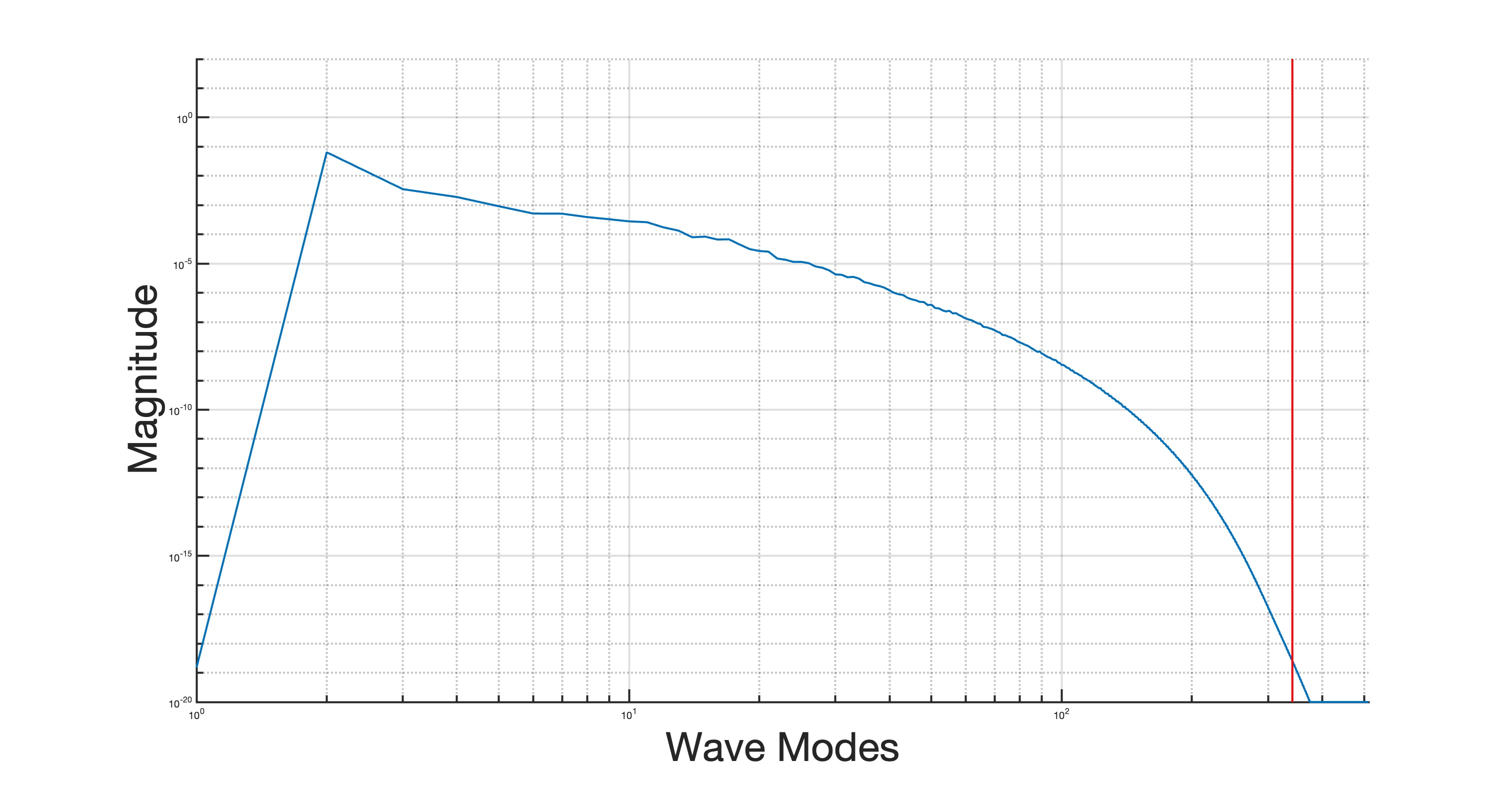
Figure 1. Energy spectrum of the initial data with $\nu=0.0001$, $G=500,000$, and $\Delta t=0.001$. The vertical red line is the 2/3 dealiasing cutoff as $\frac{2}{3}\frac{N}{2}=341.\overline{3}.$

We emphasize that implicit Euler for the time-stepping was chosen for its simplicity and its ability to accommodate large values of $\mu$, which is crucial for this study. The implicit treatment of the AOT feedback-control term allowed us to relax the CFL condition that is typically present in explicit implementations as $\mu\lesssim\frac{2}{dt}$, where $dt$ is size of the time step, thus facilitating the exploration of the $\mu\rightarrow\infty$ regime.

In order to test each method of data assimilation described in the previous sections, we performed a series of “identical twin” experiments. These experiments are commonly used to test methods of data assimilation and involve running two separate simulations, one for the “truth” and one which uses data assimilation to attempt to recover said truth. These simulations are run in the same time loop, with the reference solution being utilized to generate observational data for the data assimilation process.

Additionally, in our study, we examine two different paradigms of observational data, deterministic and noisy observations. The deterministic observations are direct observations of the true state, whereas the noisy observations are polluted with Gaussian white noise. For details on how the noisy observations are generated, see Section 4.3.

4.2. Convergence of Nudging to Synchronization – Deterministic Observations

In this section we describe the results of various numerical tests comparing rates of convergence across a range of $\mu$-values. In all of the trials discussed below, we initialize all schemes with identical observational data that is given by a low-mode Fourier projection of the truth solution. We note that while all methods should work with arbitrary initial conditions, we initialize all tests with the first set of observational data in order to establish initialization as a control variable for our experiments.

In Figure 3, we see that when using observational data from the lowest 100 Fourier modes, we obtain convergence to machine precision for all $\mu\geq 1$. In contrast, (see Figure 2) when too few Fourier modes are observed, we do not obtain convergence to the reference solution. Regardless, as $\mu$ increases, we see an improvement in the observed error, thus confirming the theoretical analysis. Indeed, as we send the value of $\mu$ towards infinity, the observed error converges to the observed error of the synchronization filter to machine precision

When enough Fourier modes are observed we see the expected behavior for both the synchronization and nudging schemes. That is, we see in Figure 3 that all methods exhibit exponential convergence in time to the reference solution in both the observed and unobserved errors. Moreover, in Figure 4 we see that this same behaviour occurs when the initial data for the nudging scheme is chosen to be something other than the reference solution, in this case we use zero initial data. We see in Figure 4 that when we initialize the nudged equations with something different than the observations at the initial time, the only effect is found in the during the initial period for the observed error, where the value of $\mu$ is found to determine the initial rate of rapid convergence, as well as the error level at which the error transitions from the initial rate to a slower but still exponential rate of decay.

We also investigated the complementary limit, as $\mu$ decreases to $0$, the results of which are presented in Figure 5. We point out that in Figure 5, the error plotted is not $\norm{u-\tilde{v}}_{L^{2}}$, as it is in all other plots. Instead the error here is $\norm{\tilde{u}-\tilde{v}}_{L^{2}}$, where $\tilde{u}$ is the 2D NSE solution that is initialized at $t_{0}$ with zero initial data. We note that here we have initialized $\tilde{v}$ with zero initial data, and so one explicitly recovers $\tilde{u}$ in the case of $\mu=0$. When $\mu\neq 0$ we can see that the error in both observed and unobserved modes increases at each fixed time as once increases the value of $\mu$, once again, consistent with expectation.

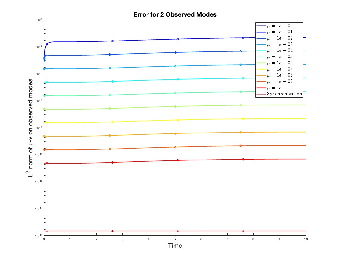
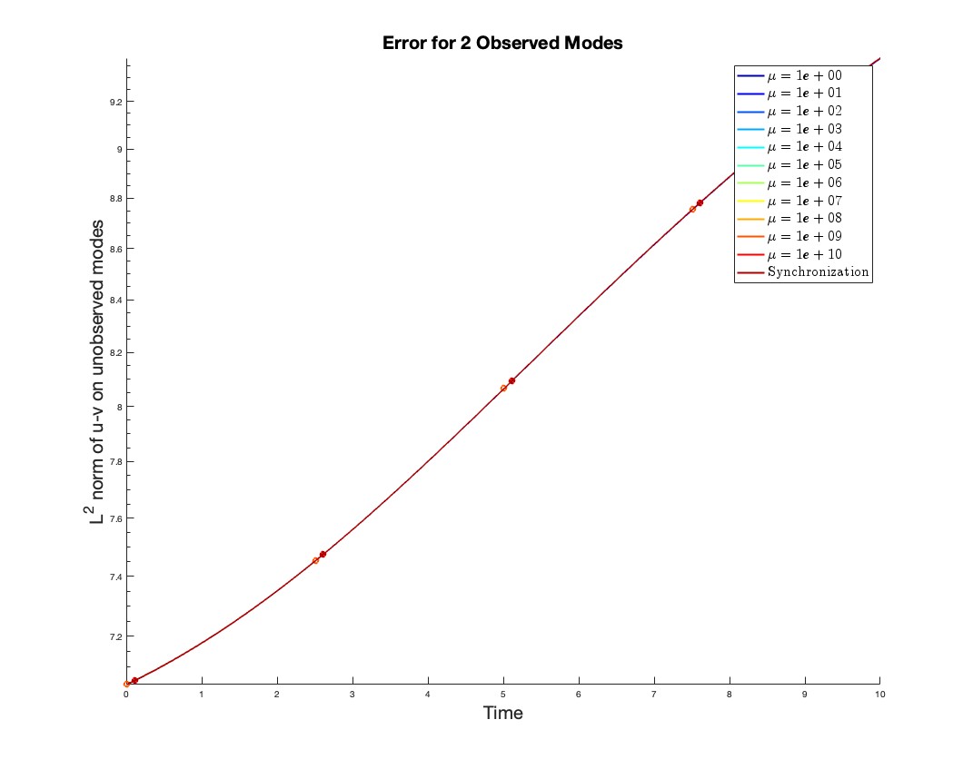
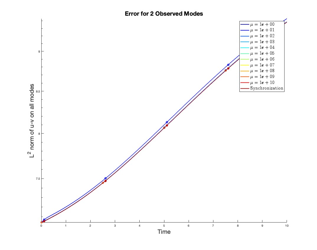
Figure 2. Error over time for different $\mu$ values for lowest 2 modes observed. Errors plotted here are low mode error (left), high mode error (middle), and total error (right), as measured by the $L^{2}$ norm. We note that the synchronization filter ($\mu=\infty$) achieves the smallest total error among all values of $\mu$.

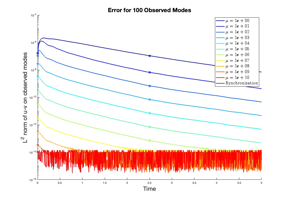
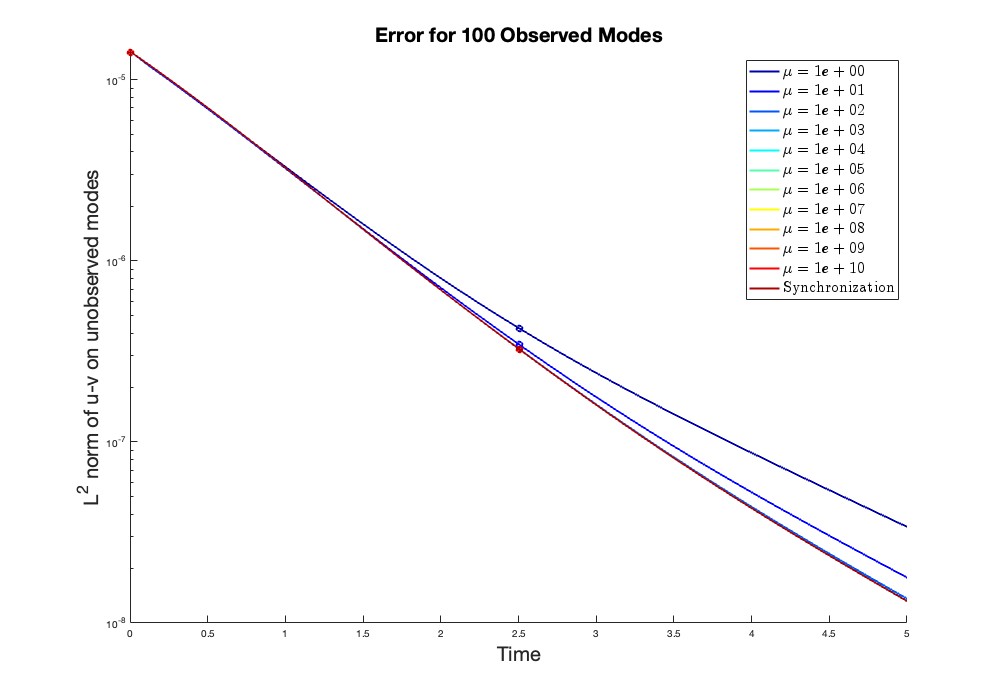
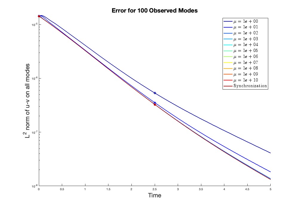
Figure 3. Error over time for different $\mu$ values assuming lowest 100 modes are observed. The nudging methods here were initialized with the low modes of the observed reference solution. Errors plotted here are low mode error (left), high mode error (middle), and total error (right), as measured by the $L^{2}$ norm.

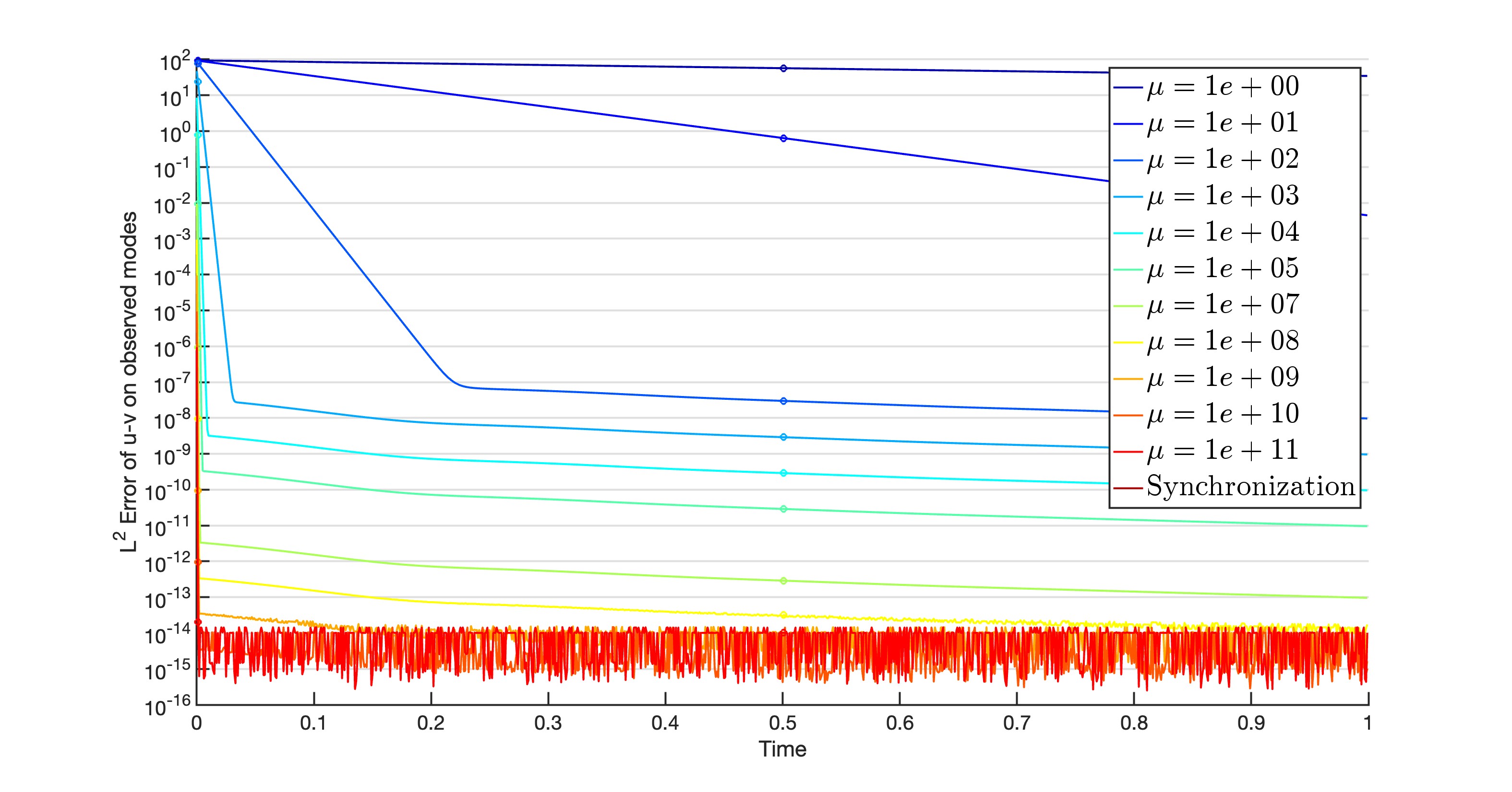
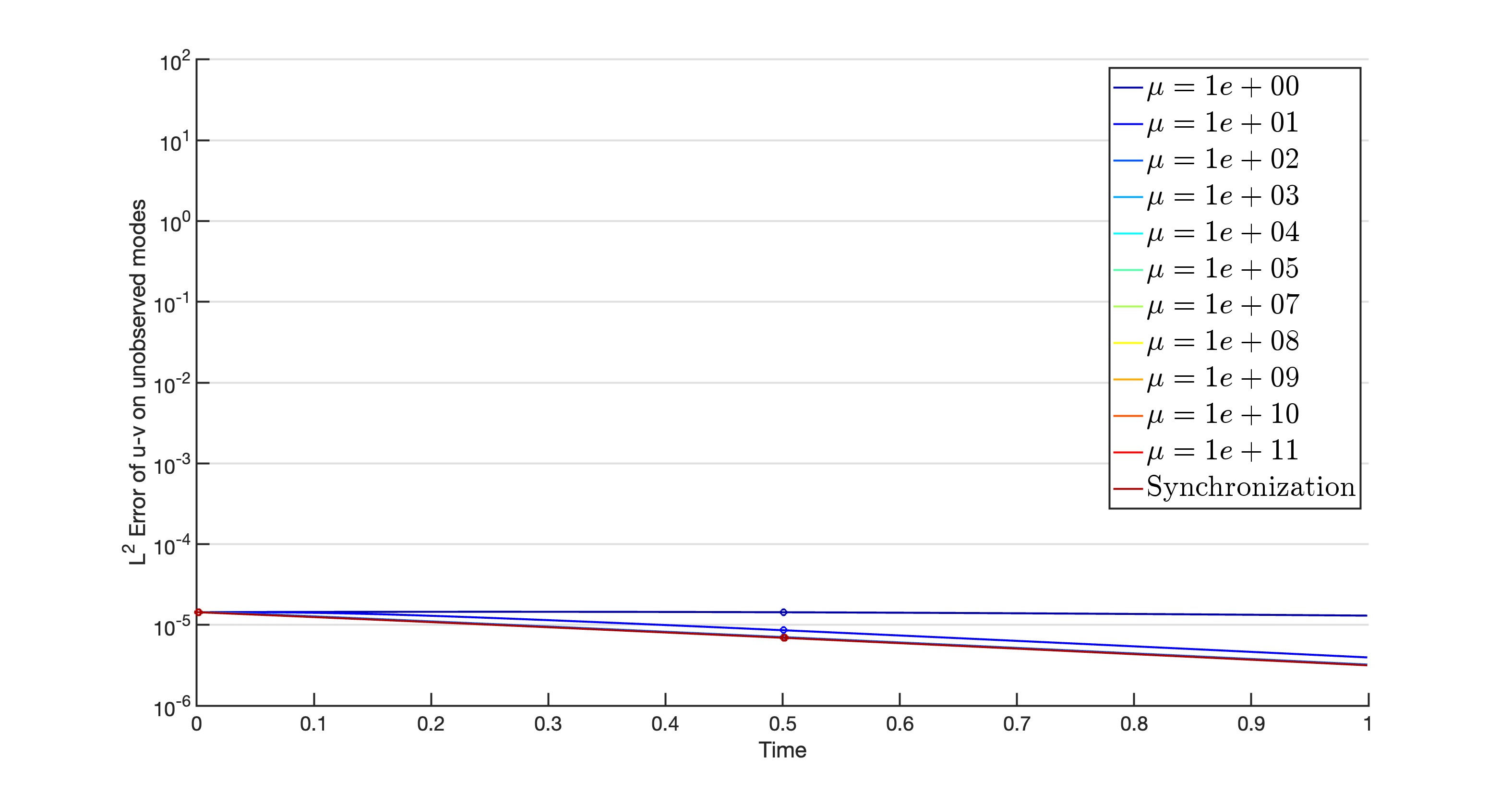
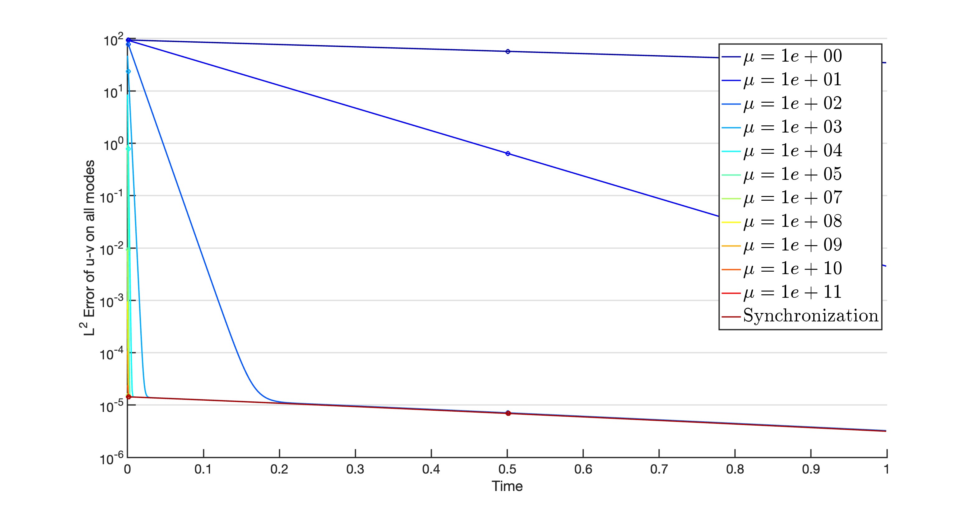
Figure 4. Error over time for different $\mu$ values assuming lowest 100 modes observed. The nudging methods were initialized with zero initial data. Errors plotted here are low mode error (left), high mode error (middle), and total error (right), as measured by the $L^{2}$ norm.

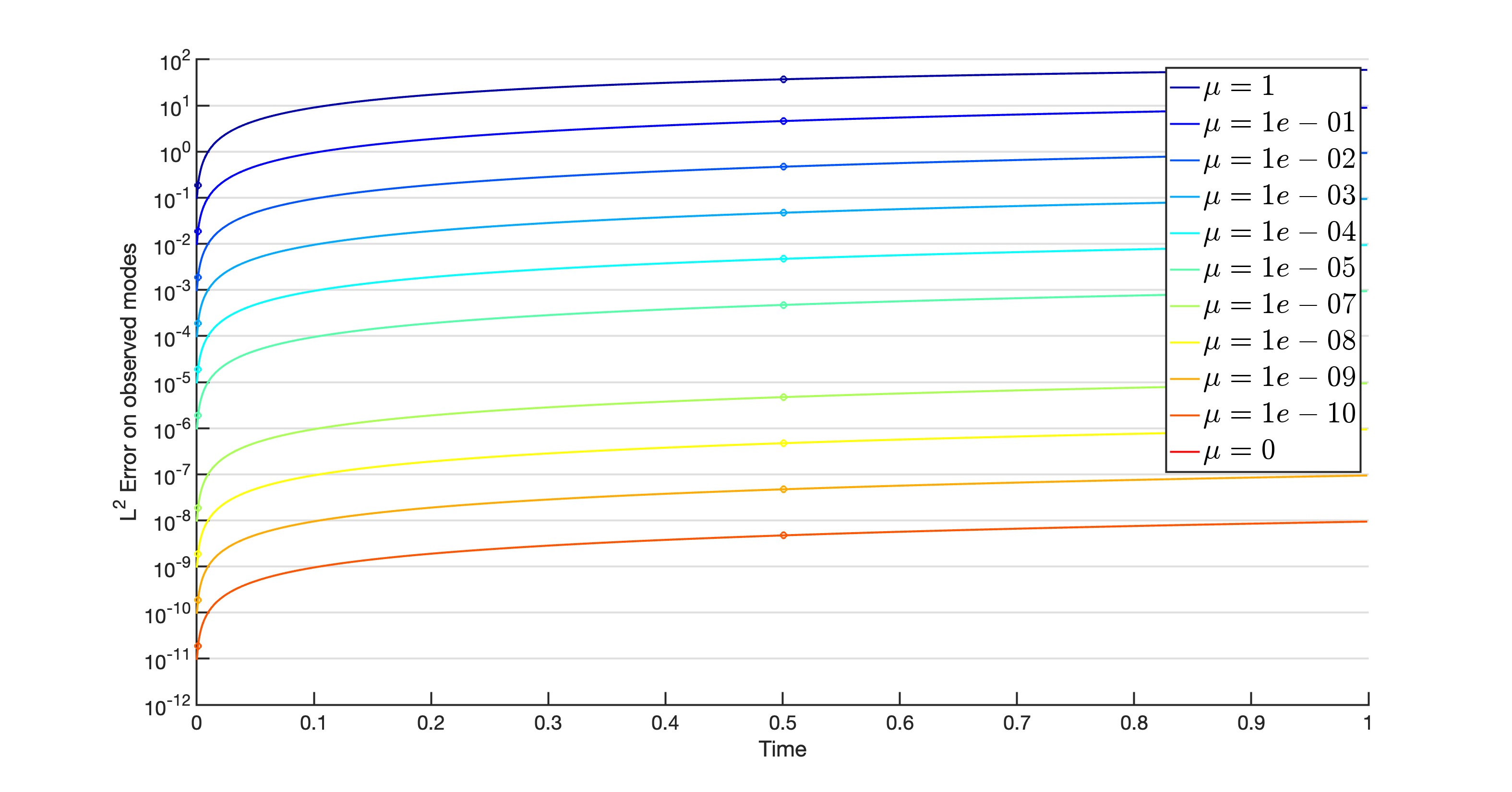
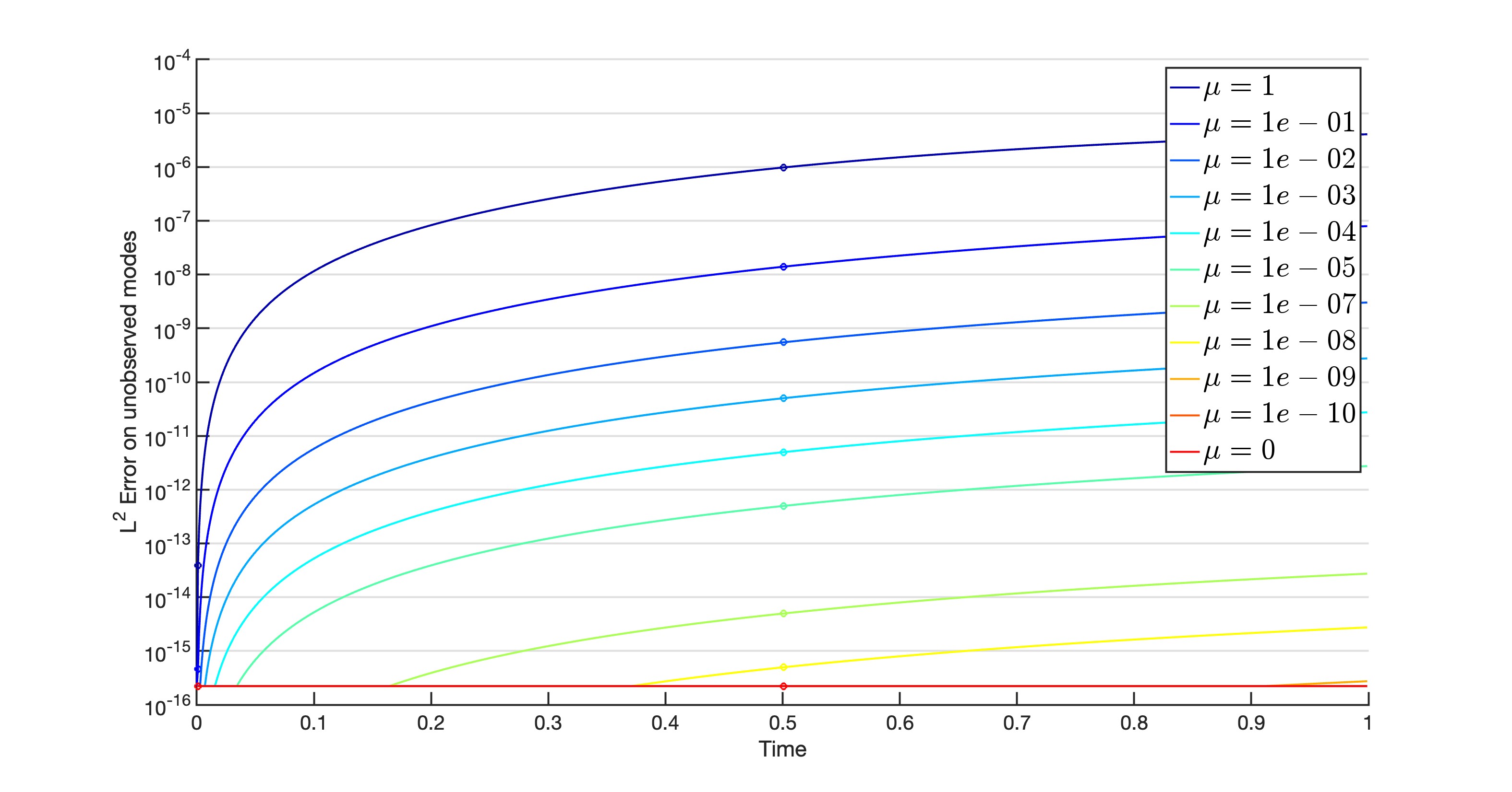
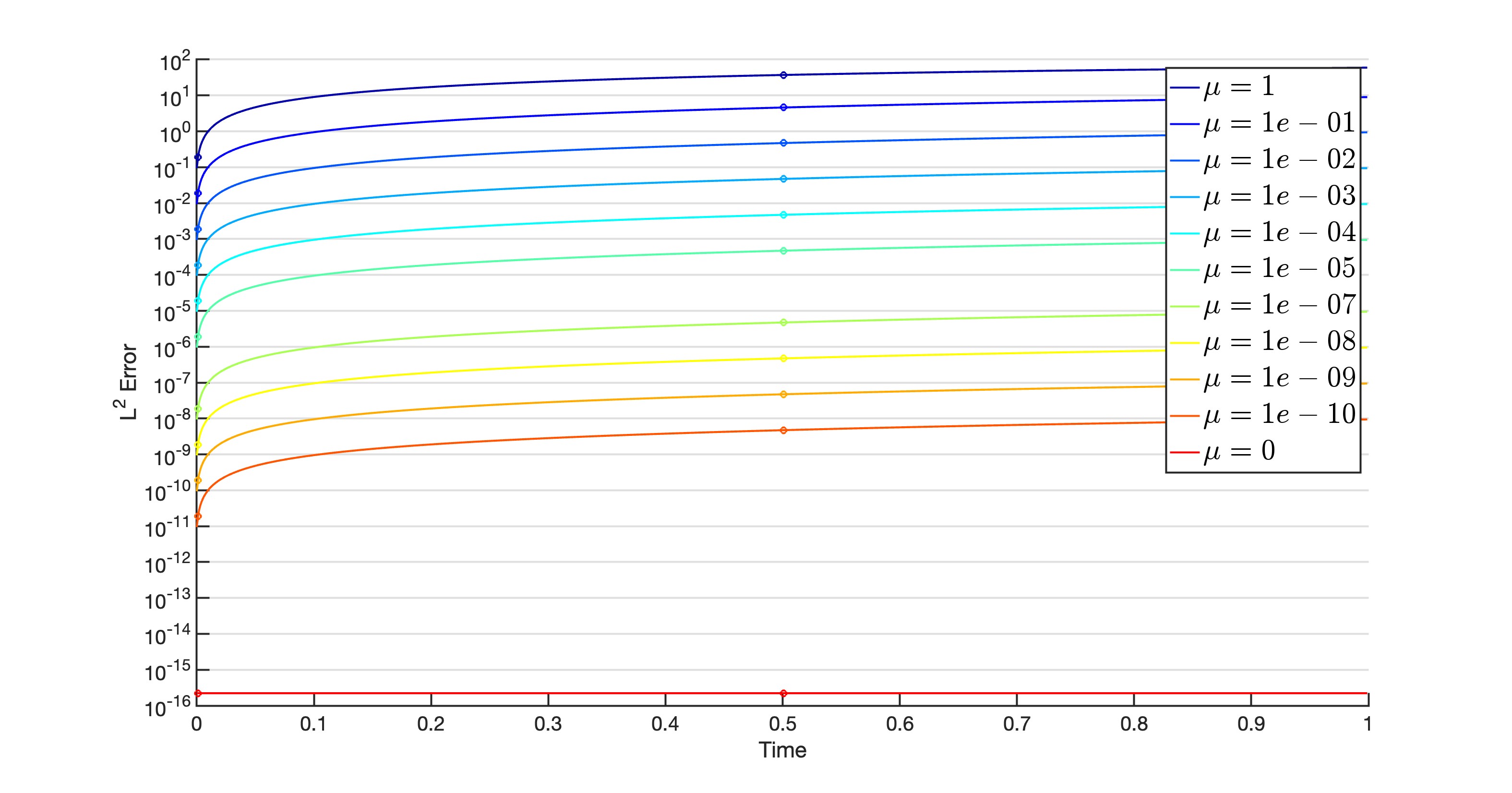
Figure 5. Error over time for different $\mu$ values assuming lowest 100 modes observed. The nudging methods were initialized with zero initial data. Error here is measured as $\norm{\tilde{u}-v}_{L^{2}}$, where $\tilde{u}$ is the solution of NSE, which formally corresponds to the un-nudged solution with zero initial data. Errors plotted here are low mode error (left), high mode error (middle), and total error (right), as measured by the $L^{2}$ norm.

4.3. Convergence of Nudging to Synchronization - Stochastic Observations

In the comparison of these data assimilation schemes, a vital test is to see how capable they are of handling imperfections in the observational data. To assess this, we utilized observational data polluted with Gaussian white noise.

The modified observational data $u_{obs}$, is formulated as follows:

$$u_{obs}(t)\mathrel{\mathop{\mathchar 58\relax}}=P_{N}u(t)+\eta(t),$$

where $\eta$ represents the observational noise injected at each timestep. This noise $\eta$ is constructed as a matrix of random complex coefficients, each corresponding to lower Fourier mode frequencies:

$$\eta(t)=\sum_{\absolutevalue{\vec{k}}=1}^{N}\hat{\eta}_{\vec{k}}(t)e^{i\pi\vec{k}}.$$ (4.2)

At each timestep, the coefficients $\hat{\eta}_{\vec{k}}$ are randomly generated as Gaussian white noise variables, each with a standard deviation of $\sigma=0.1$. It is important to note that $\hat{\eta}_{\vec{k}}$ are complex numbers, having both real and imaginary components generated such that $\real\eta,\imaginary\eta\sim N(0,0.01)$.

In generating $\eta$ as Gaussian white noise in Fourier space, we took additional steps to ensure the symmetry of the noise matrix. This is critical for obtaining real coefficients upon employing the inverse Fourier transformation in our numerics. After the initial generation of the noise, we create a symmetric matrix by constructing its Hermitian conjugate. This was done by mirroring the noise matrix about its center using a combination of rotation and complex conjugation. These operations ensure the Hermitian symmetry of the noise matrix, which ultimately guarantees real values in the spatial domain after applying the inverse Fourier transform.

Algorithm 1 Adaptive $\mu$ Scheme

1:$\tilde{u}$, the observations of the reference solution, $u$, polluted by observational noise.

2:$N$, the number of Fourier modes observed by the interpolant, $P_{N}$.

3:$tol$, a tolerance level determining when apply adaptive scheme.

4:$\mu=1e+5$ %% Initialize with large $\mu$

5:$update\_counter=0$ %% Initialize counter to delay slope calculation

6:for $t_{i}=t_{0}\mathrel{\mathop{\mathchar 58\relax}}\Delta t\mathrel{\mathop{\mathchar 58\relax}}T$ do

7:     $v(t_{i})=M(v,P_{N}(\tilde{u}(t_{i}),\mu)$ %% Evolve DA scheme forward.

8:     $E_{obs}(t_{i})=\norm{P_{N}(\tilde{u}(t_{i})-v(t_{i}))}_{L}^{2}$

9:     $update\_counter=update\_counter+1$

10:     if $update\_counter>5$ then

11:         $slope=\frac{\log(E_{obs}(t_{i-5}))-\log(E_{obs}(t_{i}))}{5\Delta t}$

12:         if $slope>tol$ then

13:              $\mu=\mu/10$

14:              $update\_counter=0$

15:         end if

16:     end if

17:end for

Since value of $\mu$ dictates the convergence levels achieved in the nudging algorithm, this led us to investigate the effect of using an adaptive value of $\mu$. As one can see in Figure 8, the error appears to converge to a static level determined at least in part by $\mu$. However, one can notice that while the resulting convergence for large $\mu$ is overall worse than for small $\mu$ values, the convergence at initial times is noticeably better (see Figure 7). It appears the value of $\mu$ corresponds to a static error level, yet large values of $\mu$ still correspond to faster convergence to the fixed error level. Thus, we utilized an adaptive $\mu$ scheme in order to capitalize on both the fast initial convergence of large $\mu$’s and the better overall convergence obtained for smaller $\mu$ values.

Remark 4.1.

We point out that although $\mu$ drives synchronization, it is simultaneously amplifies observational noise, thus leading to substantial loss in precision when $\mu$ is taken too large. This phenomenon was quantified in the theoretical work [BOT15], which found that the expected error should grow no more than $\mu|\sigma|^{2}$. Within our numerical setup, we see that the constant-$\mu$ strategy saturates the analytical error bounds established in [BOT15]. However, the adaptive-$\mu$ strategy proposed here appears to beat this bound by a measurable factor. We interpret the adaptive-$\mu$ strategy depends only on observable quantities, we view this result as being optimal.

To dynamically adjust the parameter $\mu$ based on the evolution of errors, we opted for a relatively simple approach given in Algorithm 1. The main idea is to approximate the slope of the error on the low modes using the error on the low modes from $5$ timesteps previous. The choice of using the data from $5$ timesteps ago is somewhat arbitrary, as the importance of this scheme is to calculate the slope of the observed error. We see that the low-mode error tends to behave as follows:

$$\norm{P_{N}u(t)-P_{N}v(t)}_{L^{2}}^{2}\sim\max\left\{e^{-kt},C(\mu,\sigma_{O})\right\},$$

where $k>0$ is some decay constant, and $C(\mu,\sigma_{O})$ is a constant depending on $\mu$ and $\sigma_{O}$. This error tends to decay exponentially until it reaches a level of precision determined by $\mu$ and $\sigma_{O}$, after which it remains roughly constant with fluctuations due to the noise in the observations. In the adaptive algorithm, we therefore allow $\mu$ to be sensitive to the observed error and check whether it decays exponentially or remains roughly constant. If the error is roughly constant, then we decrease the value of $\mu$ in order to effect a decrease in the value of $C(\mu,\sigma_{O})$. Ultimately, we found that the proposed adaptive $\mu$ scheme increases the overall precision in the long term while maintaining fast initial convergence levels seen with larger $\mu$ values. We note that we could adjust this algorithm to allow for $\mu$ to increase, however we found this problematic as the value of $\mu$ inflates the observational error, leading to loss of precision if $\mu$ is ever increased in value. It is worth noting that this scheme can be readily adapted for spatially-dependent $\mu$ simply by having $\mu$ depend on each individual wave-number and calculating the observed error in Algorithm 1 on each Fourier mode.

Remark 4.2.

In a recent work [CFLS24], adaptive $\mu$ schemes were also studied in the context of the 2D and 3D NSE. Two such schemes were proposed, the first of which (also called Algorithm 1) is similar to the one considered in the present article, but with one notable difference: the scheme considered there allows for the value of $\mu$ to increase when errors have inflated in the next time step, whereas the scheme considered here does not.

It is important to point out, however, that their tests are carried out in a regime where the nudging algorithm is not expected to synchronize with the reference solution. They observe that their adaptive scheme tends to increase $\mu$ in time. Since their observations are perfect, i.e., noise-free, the behavior of their adaptive scheme is consistent with the fact that the direct-replacement algorithm should perform the best since the dynamics on the low-modes are exact. This is verified by the results presented in Figure 2.

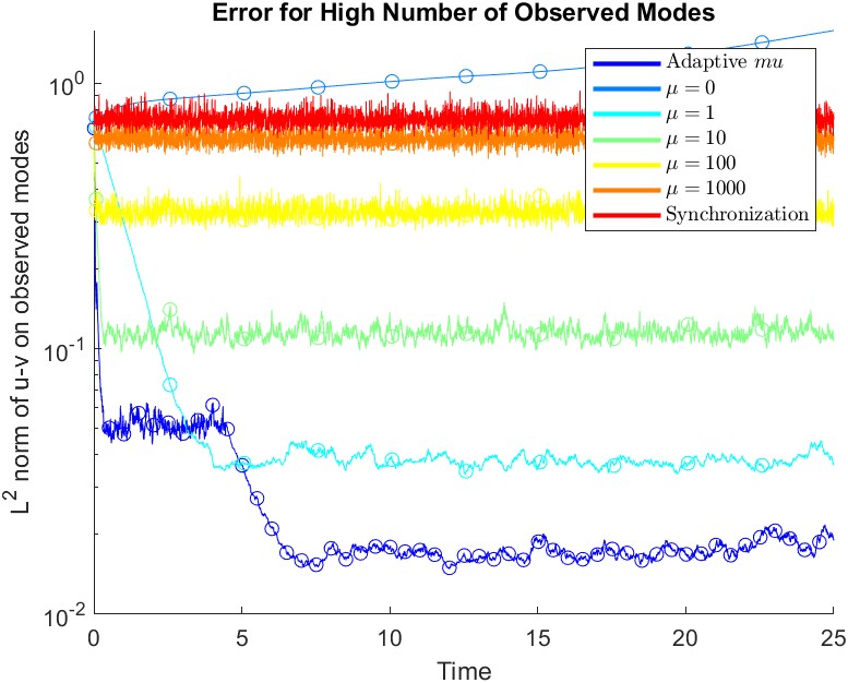
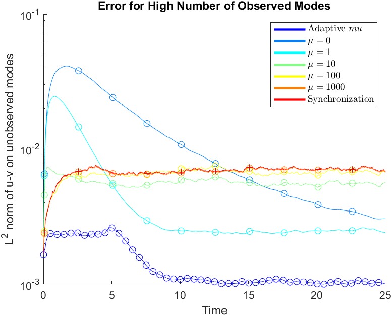
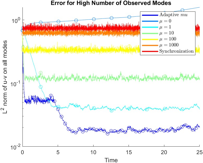
Figure 6. Error over time for different $\mu$ values for a single trial with observations polluted with measurement error. Errors plotted here are low mode error (left), high mode error (middle), and total error (right), as measured by the $L^{2}$ norm.

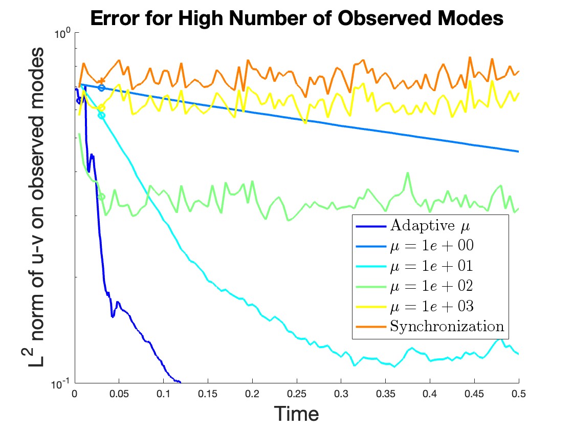
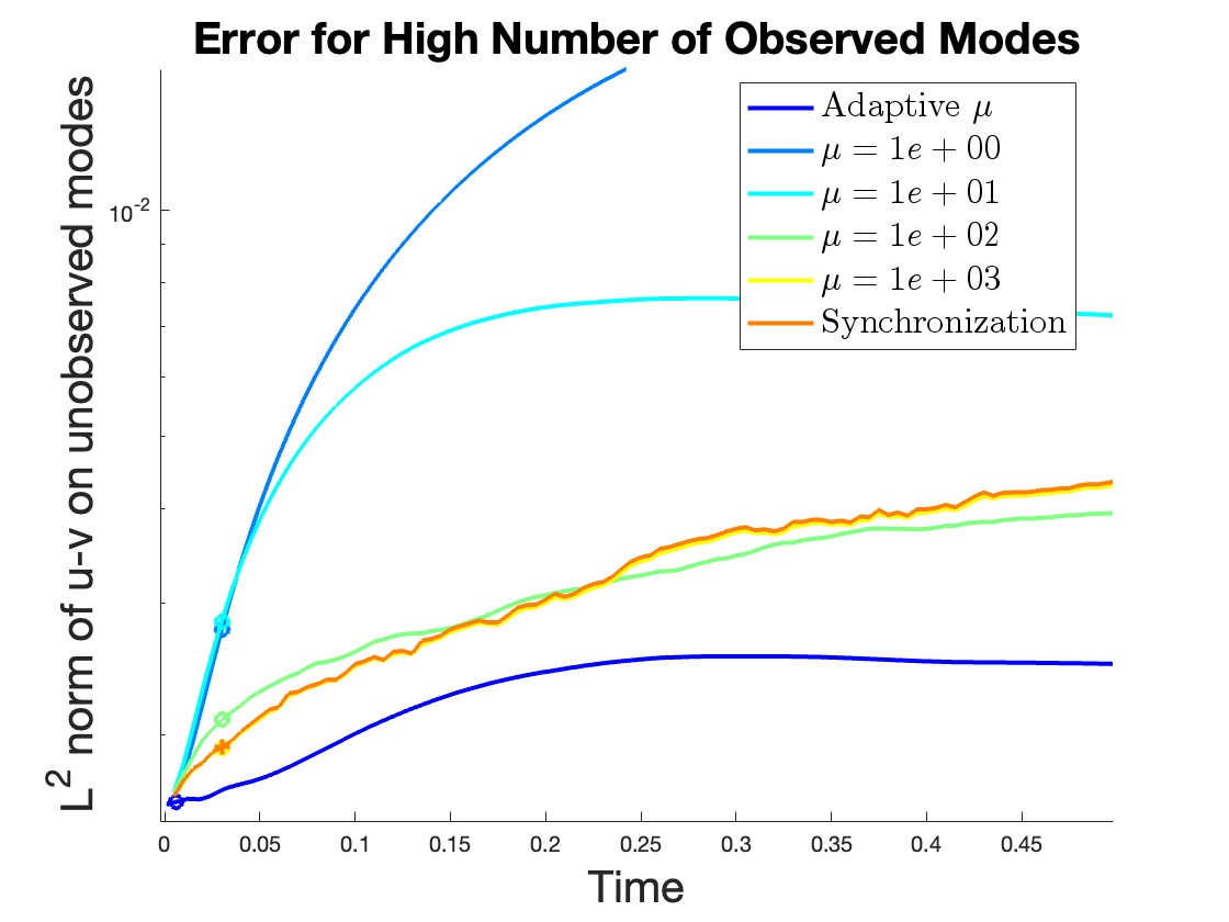
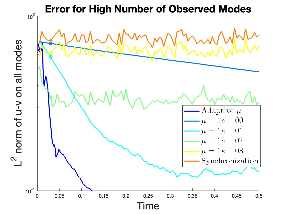
Figure 7. Error over time for different $\mu$ values for a single trial with observations polluted with measurement error. Errors plotted here are low mode error (left), high mode error (middle), and total error (right), as measured by the $L^{2}$ norm. Plots are zoomed in to feature early time development of the error.

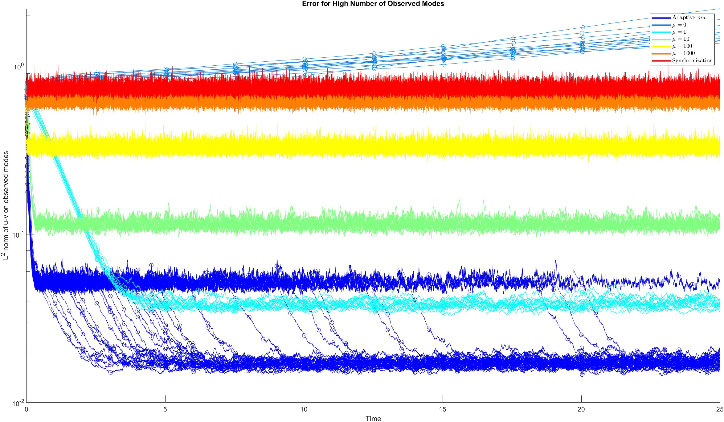
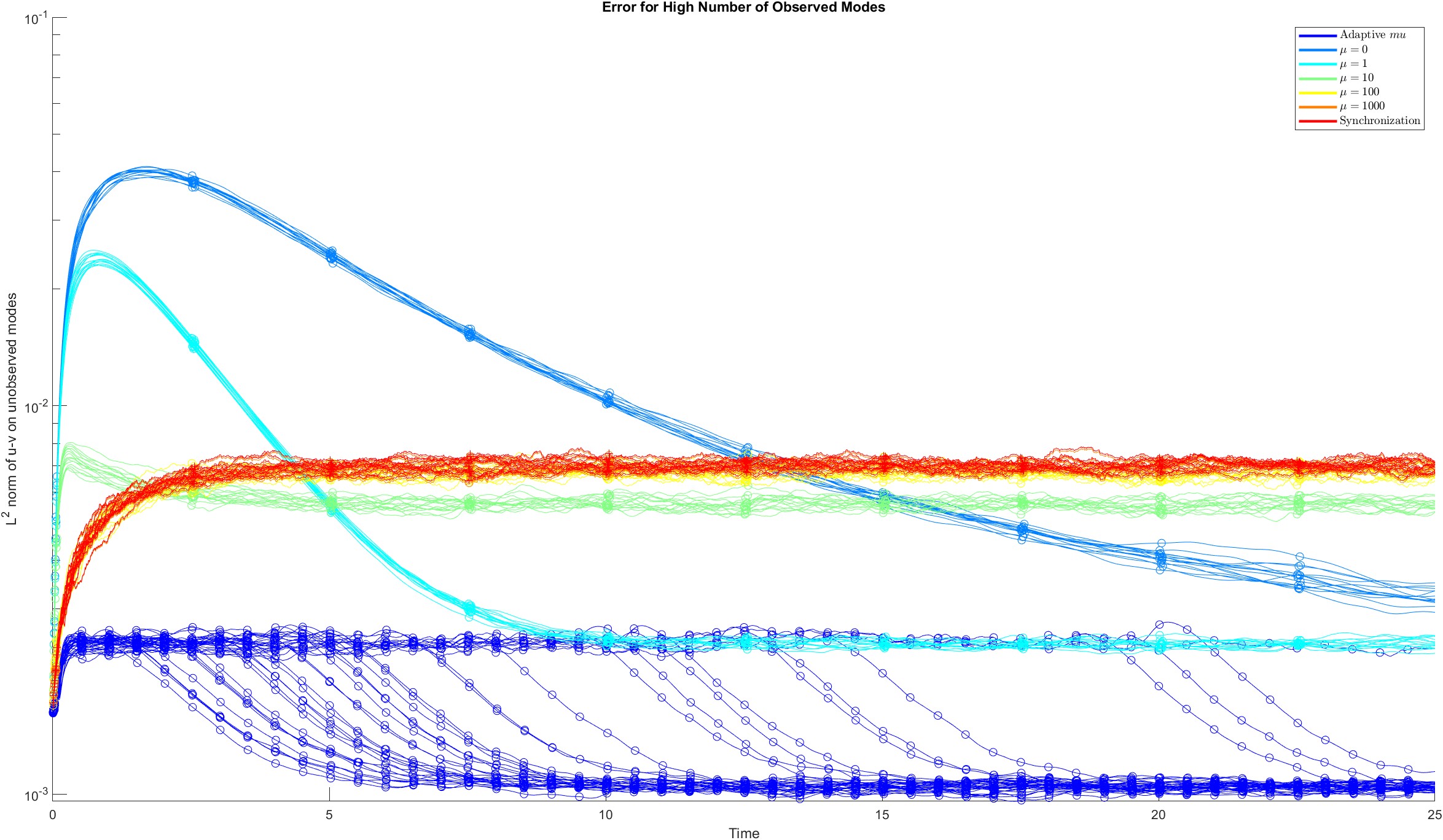
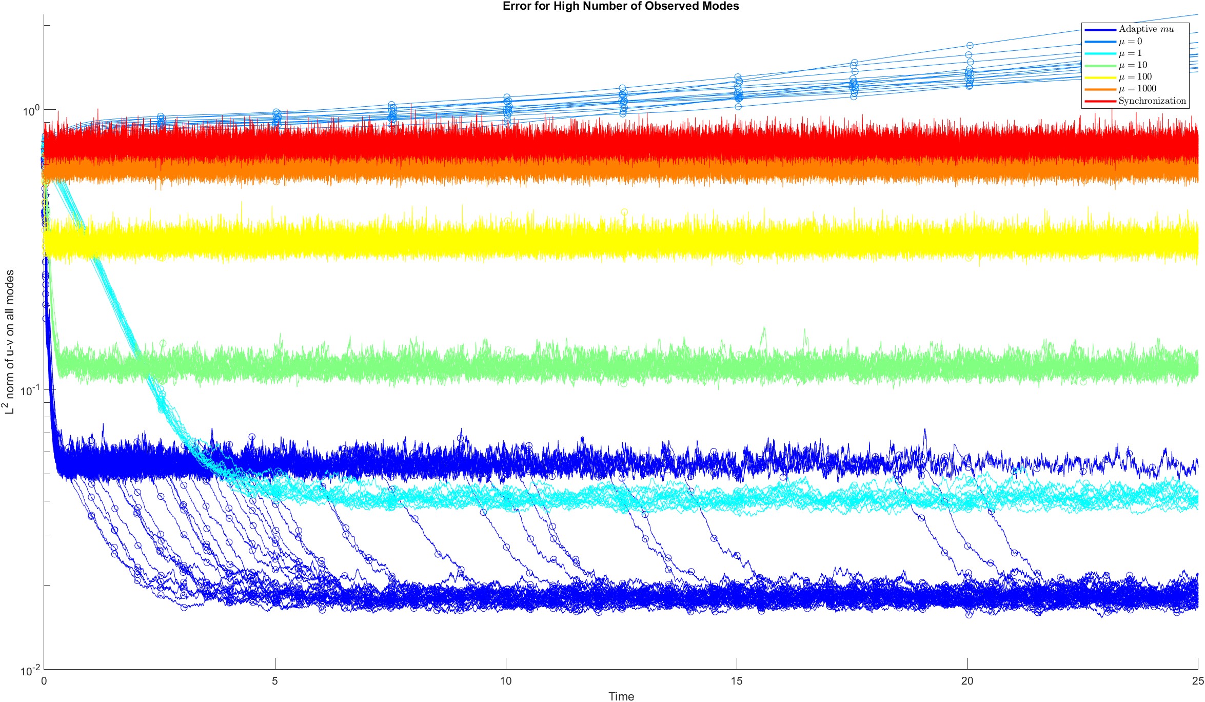
Figure 8. Error over time for different $\mu$ values for 30 trials with observations polluted with measurement error. Errors plotted here are low mode error (left), high mode error (middle), and total error (right), as measured by the $L^{2}$ norm.

Acknowledgments

The authors would like to thank Andrew Stuart and Edriss Titi for their encouragement and for stimulating discussions related to this work. A.F. was supported in part by the National Science Foundation through DMS 2206493. V.R.M. was in part supported by the National Science Foundation through DMS 2213363 and DMS 2206491, as well as the Dolciani Halloran Foundation.

Appendix A The Zero-Nudging Limit of the Nudging Filter

Let $f\in L^{\infty}(0,\infty;H)$. For $u_{0},\tilde{v}_{0}\in V$, and let $u,\tilde{u}$ denote the unique global-in-time strong solutions of (1.2) corresponding to $u_{0},\tilde{v}_{0}$, respectively, guaranteed by 2.1. As in Section 3, we will assume that the reference solution has evolved sufficiently far in time to satisfy the estimates (2.15) at $t=0$, so that without loss of generality we may suppose $t_{0}=0$ in (2.15) of 2.1. Now, given $N>0$, we consider the following set-up:

$$\frac{d\tilde{v}}{dt}+\nu A\tilde{v}+B(\tilde{v},\tilde{v}) =f-\mu P_{N}\tilde{v}+\mu P_{N}u,\quad\tilde{v}(0)=\tilde{v}_{0},$$ (A.1)

$$\frac{d\tilde{u}}{dt}+\nu A\tilde{u}+B(\tilde{u},\tilde{u}) =f,\quad\tilde{u}(0)=\tilde{v}_{0}.$$ (A.2)

Theorem A.1.

Given any $T>0$, one has

$$\lim_{\mu\rightarrow 0}\sup_{t\in[0,T]}|\tilde{v}(t;\tilde{v}_{0})-\tilde{u}(t;\tilde{v}_{0})|=0.$$

Proof.

Define $\tilde{w}=\tilde{v}-\tilde{u}$, and $w=u-\tilde{u}$. Then, $\tilde{w}$ satisfies the initial value problem

$$\frac{d\tilde{w}}{dt}-\nu A\tilde{w}+B(\tilde{w},\tilde{w})+DB(\tilde{u})\tilde{w}=-\mu P_{N}\tilde{w}+\mu P_{N}w,\qquad\tilde{w}(0)=0.$$ (A.3)

Upon taking the $H$–inner product of (A.3) with $\tilde{w}$, we obtain

$$\frac{1}{2}\frac{d}{dt}|\tilde{w}|^{2}+\nu\|\tilde{w}\|^{2}+\mu|P_{N}\tilde{w}|^{2}=-\left(B(\tilde{w},\tilde{u}),\tilde{w}\right)+\mu\left(P_{N}w,\tilde{w}\right).$$

By (2.13) and Young’s inequality, we have

$$|\left(B(\tilde{w},\tilde{u}),\tilde{w}\right)|\leq C_{L}\|\tilde{w}\|\|\tilde{u}\||\tilde{w}|\leq\nu\|\tilde{w}\|^{2}+\frac{C_{L}^{2}}{4\nu}\|\tilde{u}\|^{2}|\tilde{w}|^{2},$$

and

$$\mu|\left(P_{N}w,\tilde{w}\right)|\leq\frac{\mu}{2}|P_{N}w|^{2}+\frac{\mu}{2}|\tilde{w}|^{2}.$$

Thus, by 2.1 and (2.16), and (2.3), we have

$$\frac{d}{dt}|\tilde{w}|^{2}+\nu|\tilde{w}|^{2}+\mu|P_{N}\tilde{w}|^{2}\leq\nu\frac{C_{L}^{2}}{2}\left(\frac{\rho_{1}}{\nu}\right)^{2}|\tilde{w}|^{2}+\mu|P_{N}w|^{2},$$

which can be reduced to

$$\frac{d}{dt}|\tilde{w}|^{2}+\nu\left(1-\frac{C_{L}^{2}}{2}\left(\frac{\rho_{1}}{\nu}\right)^{2}\right)|\tilde{w}|^{2}\leq\mu|P_{N}w|^{2}.$$

By Grönwall’s inequality, and since $\tilde{w}(0)=0$, we therefore have

$$\sup_{t\in[0,T]}|\tilde{w}(t)|^{2}\leq\frac{\mu}{\nu}\left(\frac{\max\{1,e^{-\nu\mathcal{C}T}\}}{|\mathcal{C}|}\right)\sup_{t\in[0,T]}|P_{N}w|^{2}(t),$$

where $\mathcal{C}=1-\frac{C_{L}^{2}}{2}\left(\frac{\rho_{1}}{\nu}\right)^{2}$.

Next, recall that $\tilde{u}$ is the solution of the 2D NSE (A.2) while $u$ is the solution of the 2D NSE (1.1), and thus, by the standard stability argument for the 2D NSE (similar to the argument above), we have

$$\sup_{t\in[0,T]}|w(t)|^{2}\leq|w_{0}|^{2}\max\{1,e^{-\nu\mathcal{C}T}\}.$$

Thus,

$$\sup_{t\in[0,T]}|\tilde{w}(t)|^{2}\leq\frac{\mu}{\nu}\frac{\left(\max\{1,e^{-\nu\mathcal{C}T}\}\right)^{2}}{|\mathcal{C}|}|w_{0}|^{2},$$

which yields the desired conclusion. ∎

Elizabeth Carlson
Department of Computing & Mathematical Sciences
California Institute of Technology
Web: https://sites.google.com/view/elizabethcarlsonmath
Email: elizcar@caltech.edu

Aseel Farhat
Department of Mathematics
Florida State University
Email: afarhat@fsu.edu
Department of Mathematics
University of Virginia
Email: af7py@virginia.edu

Vincent R. Martinez
Department of Mathematics & Statistics
CUNY Hunter College
Department of Mathematics
CUNY Graduate Center
Web: http://math.hunter.cuny.edu/vmartine/
Email: vrmartinez@hunter.cuny.edu

Collin Victor
Department of Mathematics
Texas A&M University
Web: https://www.math.tamu.edu/people/formalpg.php?user=collin.victor
Email: collin.victor@tamu.edu

References

- [AB08] D. Auroux and J. Blum, A nudging-based data assimilation method: the Back and Forth Nudging (BFN) algorithm, Nonlinear Processes in Geophysics 15 (2008), no. 2, 305–319.
- [AB18] D.A.F. Albanez and M.J. Benvenutti, Continuous data assimilation algorithm for simplified Bardina model, Evol. Equ. Control Theory 7 (2018), no. 1, 33–52.
- [AB24] by same author, Parameter analysis in continuous data assimilation for three-dimensional Brinkman–Forchheimer-extended Darcy model, Partial Differential Equations and Applications 5 (2024), no. 4, 23.
- [AJSV08] A. Apte, C. K. R. T. Jones, A. M. Stuart, and J. Voss, Data assimilation: Mathematical and statistical perspectives, International Journal for Numerical Methods in Fluids 56 (2008), no. 8, 1033–1046.
- [ANLT16] D.A.F. Albanez, H.J. Nussenzveig Lopes, and E.S. Titi, Continuous data assimilation for the three-dimensional Navier-Stokes- model, Asymptotic Anal. 97 (2016), no. 1-2, 165–174.
- [AOT14] A Azouani, E.J. Olson, and E.S. Titi, Continuous data assimilation using general interpolant observables, J. Nonlinear Sci. 24 (2014), no. 2, 277–304.
- [ATG+17] M.U. Altaf, E.S. Titi, T. Gebrael, O.M. Knio, L. Zhao, and M.F. McCabe, Downscaling the 2D Bénard convection equations using continuous data assimilation, Comput. Geosci. 21 (2017), 393–410.
- [BB24] A. Biswas and M. Branicki, A unified framework for the analysis of accuracy and stability of a class of approximate Gaussian filters for the Navier-Stokes Equations, 2024.
- [BBJ21] A. Biswas, Z. Bradshaw, and M.S. Jolly, Data assimilation for the Navier–Stokes equations using local observables, SIAM Journal on Applied Dynamical Systems 20 (2021), no. 4, 2174–2203.
- [BCDL20] M. Buzzicotti and P. Clark Di Leoni, Synchronizing subgrid scale models of turbulence to data, Phys. Fluids 32 (2020), no. 12, 125116.
- [BFMT19] A. Biswas, C. Foias, C.F. Mondaini, and E.S. Titi, Downscaling data assimilation algorithm with applications to statistical solutions of the Navier–Stokes equations, Annales de l’Institut Henri Poincaré C, Analyse non linéaire 36 (2019), no. 2, 295–326.
- [BH23] A. Biswas and J. Hudson, Determining the viscosity of the Navier–Stokes equations from observations of finitely many modes, Inverse Problems 39 (2023), no. 12, 125012.
- [Bje04] V. Bjerknes, The problem of weather prediction, considered from the viewpoints of mechanics and physics, Meteorologische Zeitschrift 18 (1904), no. 6, 663–667.
- [BLL+13] C.E.A. Brett, K.F. Lam, K.J.H. Law, D.S. McCormick, M.R. Scott, and A.M. Stuart, Accuracy and stability of filters for dissipative pdes, Physica D: Nonlinear Phenomena 245 (2013), no. 1, 34–45.
- [BLSZ13] D. Blömker, K. Law, A. M. Stuart, and K. C. Zygalakis, Accuracy and stability of the continuous-time 3DVAR filter for the Navier-Stokes equation, Nonlinearity 26 (2013), no. 8, 2193–2219.
- [BM17] A. Biswas and V.R. Martinez, Higher-order synchronization for a data assimilation algorithm for the 2D Navier-Stokes equations, Nonlinear Anal. Real World Appl. 35 (2017), no. 1, 132–157.
- [BMO18] J. Blocher, V.R. Martinez, and E. Olson, Data assimilation using noisy time-averaged measurements, Physica D: Nonlinear Phenomena 376-377 (2018), 49–59, Special Issue: Nonlinear Partial Differential Equations in Mathematical Fluid Dynamics.
- [BOT15] H. Bessaih, E.J. Olson, and E.S. Titi, Continuous data assimilation with stochastically noisy data, J. Nonlinear Sci. 28 (2015), no. 0, 729–753.
- [BvLG98] G. Burgers, P.J. van Leeuwen, and Evensen. G., Analysis scheme in the ensemble Kalman filter, Monthly Weather Review 126 (1998), no. 6, 1719–1724.
- [CBBE18] A. Carrassi, M. Bocquet, L. Bertino, and G. Evensen, Data assimilation in the geosciences: An overview of methods, issues, and perspectives, WIREs Climate Change 9 (2018), no. 5, e535.
- [CDLMB18] P. Clark Di Leoni, A. Mazzino, and L. Biferale, Inferring flow parameters and turbulent configuration with physics-informed data assimilation and spectral nudging, Phys. Rev. Fluids 3 (2018), no. 10, 104604.
- [CDLMB20] by same author, Synchronization to big data: Nudging the Navier-Stokes equations for data assimilation of turbulent flows, Phys. Rev. X 10 (2020), 011023.
- [CFLS24] A. Cibik, R. Fang, W. Layton, and F. Siddiqua, Adaptive Parameter Selection in Nudging Based Data Assimilation, 2024.
- [CFMV24] E. Carlson, A. Farhat, V.R. Martinez, and C. Victor, Determining modes, Synchronization, and Intertwinement, 1–46.
- [CFVN50] J. G. Charney, R. Fjörtoft, and J. Von Neumann, Numerical integration of the barotropic vorticity equation, Tellus 2 (1950), no. 4, 237–254.
- [Cha51] J.G. Charney, Dynamic forecasting by numerical process, Compendium of meteorology, pp. 470–482, American Meteorological Society, Boston, MA, 1951.
- [CHJ69] J. Charney, M. Halem, and R. Jastrow, Use of incomplete historical data to infer the present state of the atmosphere, J. Atmos. Sci. 26 (1969), 1160–1163.
- [CHL20] E. Carlson, J. Hudson, and A. Larios, Parameter recovery for the 2 dimensional Navier-Stokes equations via continuous data assimilation, SIAM J. Sci. Comput. 42 (2020), no. 1, A250–A270.
- [CHL+22] E. Carlson, J. Hudson, A. Larios, V.R. Martinez, E. Ng, and J.P. Whitehead, Dynamically learning the parameters of a chaotic system using partial observations, 2022, pp. 3809–3839.
- [CJT97] B. Cockburn, D.A. Jones, and E.S. Titi, Estimating the number of asymptotic degrees of freedom for nonlinear dissipative systems, Math. Comput. 66 (1997), 1073–1087.
- [CO23] E. Celik and E. Olson, Data assimilation using time-delay nudging in the presence of Gaussian noise, Journal of Nonlinear Science 33 (2023), no. 6, 110.
- [COT19] E. Celik, E. Olson, and E.S. Titi, Spectral filtering of interpolant observables for a discrete-in-time downscaling data assimilation algorithm, SIAM J. Appl. Dyn. Syst. 18 (2019), no. 2, 1118–1142. MR 3959540
- [DDL+19] S. Desamsetti, H.P. Dasari, S. Langodan, E.S. Titi, O. Knio, and I. Hoteit, Efficient dynamical downscaling of general circulation models using continuous data assimilation, Quarterly Journal of the Royal Meteorological Society 145 (2019), no. 724, 3175–3194.
- [DLR24] A. Diegel, X. Li, and L.G. Rebholz, Analysis of continuous data assimilation with large (or even infinite) nudging parameters, 2024.
- [DTW06] G. S. Duane, J. J. Tribbia, and J. B. Weiss, Synchronicity in predictive modelling: a new view of data assimilation, Nonlinear Processes in Geophysics 13 (2006), no. 6, 601–612.
- [Eve97] G. Evensen, Advanced data assimilation for strongly nonlinear dynamics, Mon. Wea. Rev. 125 (1997), 1342–1354.
- [FGHM+20] A. Farhat, N. E. Glatt-Holtz, V.R. Martinez, S. A. McQuarrie, and J.P. Whitehead, Data assimilation in large Prandtl Rayleigh-Bénard convection from thermal measurements, SIAM J. Appl. Dyn. Syst. 19 (2020), no. 1, 510–540. MR 4065631
- [FJJT18] A. Farhat, H. Johnston, M.S. Jolly, and E.S. Titi, Assimilation of nearly turbulent Rayleigh-Bénard flow through vorticity or local circulation measurements: A computational study, J. Sci. Comput. (2018), 1–15.
- [FJKT12] C. Foias, M.S. Jolly, R. Kravchenko, and E.S. Titi, A determining form for the two-dimensional Navier-Stokes equations: the Fourier modes case, J. Math. Phys. 53 (2012), no. 11, 115623, 30.
- [FJKT14] C. Foias, M. S. Jolly, R. Kravchenko, and E. S. Titi, A unified approach to determining forms for the 2D Navier–Stokes equations - the general interpolants case, Russian Mathematical Surveys 69 (2014), no. 2, 359.
- [FJLT17] C. Foias, M.S. Jolly, D. Lithio, and E.S. Titi, One-dimensional parametric determining form for the two-dimensional Navier-Stokes equations, J. Nonlinear Sci. 27 (2017), no. 5, 1513–1529.
- [FJT15] A. Farhat, M.S. Jolly, and E.S. Titi, Continuous data assimilation for the 2D Bénard convection through velocity measurements alone, Phys. D 303 (2015), 59–66.
- [FLMW24] Aseel Farhat, Adam Larios, Vincent R. Martinez, and Jared P. Whitehead, Identifying the body force from partial observations of a two-dimensional incompressible velocity field, Phys. Rev. Fluids 9 (2024), 054602.
- [FLT16a] A. Farhat, E. Lunasin, and E.S. Titi, Abridged continuous data assimilation for the 2D Navier-Stokes equations utilizing measurements of only one component of the velocity field, J. Math. Fluid Mech. 18 (2016), no. 1, 1–23.
- [FLT16b] by same author, Data assimilation algorithm for 3D Bénard convection in porous media employing only temperature measurements, J. Math. Anal. Appl. 438 (2016), no. 1, 492–506.
- [FLT16c] by same author, On the Charney conjecture of data assimilation employing temperature measurements alone: The paradigm of 3D planetary geostrophic model, Math. of Climate and Wea. Forecasting 2 (2016), 61–74.
- [FLV22] T. Franz, A. Larios, and C. Victor, The bleeps, the sweeps, and the creeps: Convergence rates for dynamic observer patterns via data assimilation for the 2D Navier–Stokes equations, Computer Methods in Applied Mechanics and Engineering 392 (2022), 114673.
- [FMRT01] C. Foias, O. Manley, R. Rosa, and R. Temam, Navier-Stokes equations and turbulence, Encyclopedia of Mathematics and its Applications, vol. 83, Cambridge University Press, Cambridge, 2001. MR 1855030 (2003a:76001)
- [FMT16] C. Foias, C. Mondaini, and E.S. Titi, A discrete data assimilation scheme for the solutions of the 2D Navier-Stokes equations and their statistics, SIAM J. Appl. Dyn. Syst. 15 (2016), no. 4, 2019–2142.
- [FP67] C. Foiaş and G. Prodi, Sur le comportement global des solutions non-stationnaires des équations de Navier-Stokes en dimension , Rend. Sem. Mat. Univ. Padova 39 (1967), 1–34.
- [FT84] C. Foias and R. Temam, Determination of the solutions of the Navier-Stokes equations by a set of nodal values, Math. Comput. 43 (1984), no. 167, 117–133.
- [FT87] by same author, The connection between the Navier-Stokes equations, dynamical systems, and turbulence theory, Directions in partial differential equations (Madison, WI, 1985), Publ. Math. Res. Center Univ. Wisconsin, vol. 54, Academic Press, Boston, MA, 1987, pp. 55–73. MR 1013833
- [GALNR24] B. García-Archilla, X. Li, J. Novo, and L.G. Rebholz, Enhancing nonlinear solvers for the Navier–Stokes equations with continuous (noisy) data assimilation, Computer Methods in Applied Mechanics and Engineering 424 (2024), 116903.
- [GOT16] M. Gesho, E.J. Olson, and E.S. Titi, A computational study of a data assimilation algorithm for the two-dimensional Navier-Stokes equations, Commun. Comput. Phys. 19 (2016), no. 4, 1094–1110.
- [GSS93] N.J. Gordon, D.J. Salmond, and A.F.M. Smith, Novel approach to nonlinear/non-Gaussian Bayesian state estimation, IEE Proceedings F (Radar and Signal Processing) 140 (1993), 107–113(6) (English).
- [HA76] J. E. Hoke and R. A. Anthes, The initialization of numerical models by a dynamic-initialization technique, Monthly Weather Review 104 (1976), no. 12, 1551–1556.
- [HOT11] K. Hayden, E. Olson, and E.S. Titi, Discrete data assimilation in the Lorenz and 2D Navier-Stokes equations, Phys. D 240 (2011), no. 18, 1416–1425. MR 2831793
- [HTHK22] M.A.E.R. Hammoud, E.S. Titi, I. Hoteit, and O. Knio, CDAnet: A physics-informed deep neural network for downscaling fluid flows, Journal of Advances in Modeling Earth Systems 14 (2022), no. 12, e2022MS003051, e2022MS003051 2022MS003051.
- [IMT19] H.A. Ibdah, C.F. Mondaini, and E.S. Titi, Fully discrete numerical schemes of a data assimilation algorithm: uniform-in-time error estimates, IMA Journal of Numerical Analysis 40 (2019), no. 4, 2584–2625.
- [JMOT19] M.S. Jolly, V.R. Martinez, E.J. Olson, and E.S. Titi, Continuous data assimilation with blurred-in-time measurements of the surface quasi-geostrophic equation, Chin. Ann. Math. Ser. B 40 (2019), 721––764.
- [JMST18] M.S. Jolly, V.R. Martinez, S. Sadigov, and E.S. Titi, A Determining Form for the Subcritical Surface Quasi-Geostrophic Equation, J. Dyn. Differ. Equations (2018), 1–38.
- [JMT17] M.S. Jolly, V.R. Martinez, and E.S. Titi, A data assimilation algorithm for the 2D subcritical surface quasi-geostrophic equation, Adv. Nonlinear Stud. 35 (2017), 167–192.
- [JP23] M.S. Jolly and A. Pakzad, Data assimilation with higher order finite element interpolants, International Journal for Numerical Methods in Fluids 95 (2023), no. 3, 472–490.
- [JST15] M.S. Jolly, T. Sadigov, and E.S. Titi, A determining form for the damped driven nonlinear Schrödinger equation–Fourier modes case, J. Differential Equations 258 (2015), 2711–2744.
- [JST17] by same author, Determining form and data assimilation algorithm for weakly damped and driven Korteweg-de Vries equation- Fourier modes case, Nonlinear Anal. Real World Appl. 36 (2017), 287–317.
- [JT92a] D.A. Jones and E.S. Titi, Determining finite volume elements for the 2D Navier-Stokes equations, Phys. D 60 (1992), 165–174.
- [JT92b] by same author, On the number of determining nodes for the 2D Navier-Stokes equations, J. Math. Anal. 168 (1992), 72–88.
- [Kal03] E. Kalnay, Atmospheric modeling, data assimilation and predicatability, Cambridge University Press, 2003.
- [KB61] R. E. Kalman and R. S. Bucy, New Results in Linear Filtering and Prediction Theory, Journal of Basic Engineering 83 (1961), no. 1, 95–108.
- [KT05] A-K. Kassam and L.N. Trefethen, Fourth-order time-stepping for stiff PDEs, SIAM J. Sci. Comput. 26 (2005), no. 4, 1214–1233. MR 2143482
- [Kün13] Hans R. Künsch, Particle filters, Bernoulli 19 (2013), no. 4, 1391 – 1403.
- [LDT86] F.X. Le Dimet and O. Talgrand, Variational algorithms for analysis and assimilation of meteorological observations: theoretical aspects, Tellus A 38A (1986), 97–110.
- [LHRV23] X. Li, E.V. Hawkins, L.G. Rebholz, and D. Vargun, Accelerating and enabling convergence of nonlinear solvers for Navier–Stokes equations by continuous data assimilation, Computer Methods in Applied Mechanics and Engineering 416 (2023), 116313.
- [Lor86] A. C. Lorenc, Analysis methods for numerical weather prediction, Quarterly Journal of the Royal Meteorological Society 112 (1986), no. 474, 1177–1194.
- [LRZ19] A. Larios, L.G. Rebholz, and C. Zerfas, Global in time stability and accuracy of IMEX-FEM data assimilation schemes for Navier-Stokes equations, Comput. Methods Appl. Mech. Engrg. 345 (2019), 1077–1093. MR 3912985
- [Lue64] D.G. Luenberger, Observing the state of a linear system, IEEE Transactions on Military Electronics 8 (1964), no. 2, 74–80.
- [Mar22] V.R. Martinez, Convergence analysis of a viscosity parameter recovery algorithm for the 2D Navier-Stokes equations, Nonlinearity 35 (2022), no. 5, 2241–2287. MR 4420613
- [Mar24] by same author, On the reconstruction of unknown driving forces from low-mode observations in the 2D Navier–Stokes equations, Proc. R. Soc. Edinb. A: Math (2024), 1–24.
- [MT18] C.F. Mondaini and E.S. Titi, Uniform-in-time error estimates for the postprocessing Galerkin method applied to a data assimilation algorithm, SIAM J. Numer. Anal. 56 (2018), no. 1, 78–110.
- [OBK18] L. Oljača, J. Bröcker, and T. Kuna, Almost sure error bounds for data assimilation in dissipative systems with unbounded observation noise, SIAM Journal on Applied Dynamical Systems 17 (2018), no. 4, 2882–2914.
- [OT03] E. Olson and E.S. Titi, Determining modes for continuous data assimilation in 2D turbulence, J. Statist. Phys. 113 (2003), no. 5-6, 799–840, Progress in statistical hydrodynamics (Santa Fe, NM, 2002). MR 2036872
- [OT08] by same author, Determining modes and Grashof number in 2D turbulence: A numerical case study, Theor. Comput. Fluid Dyn. 22 (2008), 327–339.
- [PC90] Louis M. Pecora and Thomas L. Carroll, Synchronization in chaotic systems, Phys. Rev. Lett. 64 (1990), 821–824.
- [PCL16] D. Pazó, A. Carrassi, and J. M. López, Data assimilation by delay-coordinate nudging, Quarterly Journal of the Royal Meteorological Society 142 (2016), no. 696, 1290–1299.
- [PvLG19] F.R. Pinheiro, P.J. van Leeuwen, and G. Geppert, Efficient nonlinear data assimilation using synchronization in a particle filter, Quarterly Journal of the Royal Meteorological Society 145 (2019), no. 723, 2510–2523.
- [PVS22] D. Pandya, B. Vachharajani, and R. Srivastava, A review of data assimilation techniques: Applications in engineering and agriculture, Materials Today: Proceedings 62 (2022), 7048–7052, International Conference on Additive Manufacturing and Advanced Materials (AM2).
- [PWM22] B. Pachev, J.P. Whitehead, and S.A. McQuarrie, Concurrent multiparameter learning demonstrated on the Kuramoto–Sivashinsky equation, SIAM Journal on Scientific Computing 44 (2022), no. 5, A2974–A2990.
- [Rob01] J.C. Robinson, Infinite-Dimensional Dynamical Systems, Cambridge Texts in Applied Mathematics, Cambridge University Press, Cambridge, 2001, An introduction to dissipative parabolic PDEs and the theory of global attractors. MR 1881888
- [SAS15] D. Sanz-Alonso and A.M. Stuart, Long-time asymptotics of the filtering distribution for partially observed chaotic dynamical systems, SIAM/ASA J. Uncertain. Quantif. 3 (2015), no. 1, 1200–1220. MR 3432856
- [Tem97] R. Temam, Infinite-Dimensional Dynamical Systems In Mechanics and Physics, second ed., Applied Mathematical Sciences, vol. 68, Springer-Verlag, New York, 1997. MR 1441312 (98b:58056)
- [Tre00] L.N. Trefethen, Spectral Methods in MATLAB, Software, Environments, and Tools, vol. 10, Society for Industrial and Applied Mathematics (SIAM), Philadelphia, PA, 2000. MR 1776072
- [YGJP22] C. Yu, A. Giorgini, M.S. Jolly, and A. Pakzad, Continuous data assimilation for the 3D Ladyzhenskaya model: analysis and computations, Nonlinear Analysis: Real World Applications 68 (2022), 103659.
- [You24] B. You, Continuous data assimilation for the three-dimensional planetary geostrophic equations of large-scale ocean circulation, Zeitschrift für angewandte Mathematik und Physik 75 (2024), no. 4, 147.
- [ZNL92] X. Zou, I. M. Navon, and F. X. Ledimet, An optimal nudging data assimilation scheme using parameter estimation, Quarterly Journal of the Royal Meteorological Society 118 (1992), no. 508, 1163–1186.
- [ZRSI19] C. Zerfas, L.G. Rebholz, M. Schneier, and T. Iliescu, Continuous data assimilation reduced order models of fluid flow, Computer Methods in Applied Mechanics and Engineering 357 (2019), 112596.